Evaluating Remote Sensing Products for Pasture Composition and Yield Prediction

Abstract

Vegetation and soil indices are able to indicate patterns of gradual plant growth. Therefore, productivity data may be used to predict performance in the development of pastures prior to grazing, since the morphology of the pasture follows repetitive cycles through the grazing of animals. Accordingly, in recent decades, much attention has been paid to the monitoring and development of vegetation by means of remote sensing using remote sensors. The current study seeks to determine the differences between three remote sensing products in the monitoring and development of white clover and perennial ryegrass ratios. Various grass and legume associations (perennial ryegrass, Lolium perenne, and white clover, Trifolium repens) were evaluated in different proportions to determine their yield and relationship through vegetation and soil indices. Four proportions (%) of perennial ryegrass and white clover were used, being 100:0; 90:10; 80:20 and 70:30. Likewise, to obtain spectral indices, a Spectral Evolution PSR-1100 spectroradiometer was used, and two UAVs with a MAPIR 3W RGNIR camera and a Parrot Sequoia multispectral camera, respectively, were employed. The data collection was performed before and after each cut or grazing period in each experimental unit, and post-processing and the generation of spectral indices were conducted. The results indicate that there were no significant differences between treatments for yield or for vegetation indices. However, there were significant differences in the index variables between sensors, with the spectroradiometer and Parrot obtaining similar values for the indices both pre- and post-grazing. The NDVI values were closely correlated with the yield of the forage proportions (R² = 0.8948), constituting an optimal index for the prediction of pasture yield.

1. Introduction

The profitability of a livestock farm depends on the quality of the feed, which, if not managed in a technical manner, may affect production severely; therefore, improving pasture production technology is essential [1,2,3,4,5,6]. Traditional techniques based on field measurements are the most accurate methods to collect data on crops and their botanical content; however, they are conditioned by the time of information collection, the size and destruction of the sample and the difficulty of access [7,8,9,10]. Consequently, in recent decades, remote sensing has become a fundamental tool for the development of new precision agriculture and livestock farming techniques [11,12,13,14,15,16,17].

Remote sensing is considered a tool that allows for obtaining small- or large-scale information about an object or phenomenon, analyzing data acquired through remote sensors that do not remain in direct contact with the object [18,19,20]. Remote sensing methods are a great tool with great potential for predicting, controlling and improving the productivity of crops, pastures and forage [21,22,23,24,25].

The information available for monitoring and developing forage proportions in the Ecuadorian highlands using remote sensors is very scarce [26,27,28]. This means that most of the necessary technological equipment for their application is unavailable, making it necessary to use data obtained from other countries [29,30]. Among the relevant technologies are the unmanned aerial vehicle (UAV), which is a good choice as a tool for precision agriculture [31,32,33,34,35,36]. Since UAVs are devices controlled by a remote control, they allow for obtaining information from inaccessible sites [37,38,39,40]. Currently, UAVs have sensors that allow for collecting high-definition photographs from which multispectral information on the study area can be obtained [41,42,43,44].

Remote sensing uses soil and vegetation indices such as the normalized difference vegetation index (NDVI), bare soil index (BSI), coloration index (CI) and soil-adjusted vegetation index (SAVI) [45,46,47,48,49,50]. These are considered important sources of information for the knowledge, management and control of the territory, since they provide data on the behavior of crops and the temporal evolution of variables related to development, biological activity, diagnosis of physiological parameters, determination of variables, percentage of coverage and other agricultural applications [51,52,53,54].

These indices are derived from reflectance values in specific regions of the electromagnetic spectrum, primarily the red, near-infrared (NIR) and shortwave infrared (SWIR) bands. For example, NDVI exploits the strong absorption of red light by chlorophyll and the high reflectance of NIR by healthy vegetation, making it a reliable indicator of plant vigor. SAVI incorporates a soil brightness correction factor to improve sensitivity in areas with sparse vegetation. BSI combines visible and SWIR bands to detect bare soil exposure, while CI uses red-edge and NIR reflectance to estimate chlorophyll content, which is directly related to photosynthetic activity and yield potential. These spectral mechanisms explain why such indices are widely used in yield prediction and crop monitoring.

There are some studies with remote sensors in which the spectral response of the pasture is analyzed with respect to its botanical composition, such as [55], in which a pasture quality index (PQI) is calculated by the principal component analysis (PCA) method and one of the variables considered is the composition of the pasture, and [56], in which after estimating the quality and quantity of the pasture with hyperspectral cameras and machine learning, the author recommends extending the study to legume-grass configurations. The importance of RS techniques for yield prediction has been scientifically evidenced [56,57], and UAV sensors are increasingly used for this purpose [58,59,60,61,62,63].

Although various methods and techniques have been proposed to estimate composition and productivity, the effectiveness of these sensors in performing this task has not been compared in depth. The performance of sensors with modified cameras has not been studied in depth with respect to cameras with separate bands. However, ref. [64] analyzed the effectiveness of predicting chlorophyll with vegetation indices taken from modified cameras (MAPIR) and Parrot cameras, concluding that the split-band camera was more effective. Although this method has limitations, its low cost and accessibility can be a useful and valid tool for farmers in areas with low economic resources. However, there is still a lack of comparative studies evaluating the effectiveness of different types of spectral sensors, particularly in mixed grass–legume pastures and in regions like the Ecuadorian highlands, limiting the development of accessible and accurate tools for pasture monitoring.

The main objective of this research is to analyze the performance of three spectral sensors (a modified RGNIR camera, a multispectral camera with separate bands, and a spectroradiometer) in estimating the proportions and development of white clover and perennial ryegrass. To this end, a study was conducted using three remote sensors to monitor the proportions of perennial ryegrass and white clover in a forage mixture. By evaluating botanical composition and yield across four harvests, we aimed to explore their relationship with key vegetation and soil indices, including NDVI, BSI, CI, SAVI, and AVI. This approach seeks to enhance the accuracy of yield estimation in grass–legume pastures using UAV-based remote sensing, contributing to more efficient and sustainable pasture management.

2. Materials and Methods

The proposed research has a variety of steps involved in the development of the applied methodology, and each part is better understood when expressed in a corresponding flow chart (Figure 1).

2.1. Location of the Experimental Site and Flow Chart

This research was performed in lot 31 of the National Livestock and Pasture Program of the Santa Catalina Experimental Station (E.E.S.C) in the Province of Pichincha, central Ecuador (Figure 2). This site is located at an altitude of 3058 m above sea level within the Inter-Andean Valley, surrounded by a variety of volcanoes [65,66]. The climatic zone is characterized by being humid–temperate, with a relative humidity of 79%, an average annual temperature of 12 °C and an average annual precipitation of 1300 mm [67]. Our research approach was as follows.

2.2. Plant Material and Sample Design

The forage mixture used in this study consisted of perennial ryegrass (Lolium eterna) and white clover (Trifolium repens), which represent the typical composition of pastures in the central highlands of Ecuador. Perennial ryegrass was selected for its proven adaptability to the region’s soil and climatic conditions, ensuring stable establishment and growth. White clover was included to promote uniform coverage within the sward, as its rhizomatous growth enables even spatial distribution without competing aggressively for space or resources. This combination reflects common agronomic practices and provides a representative model for evaluating pasture vigor and yield under local conditions [68,69,70,71,72]. Thus, the factors under study included four different planting proportions, in which the grass seeds (Ohau perennial ryegrass) in association with legume (Giant Ladino white clover) were used in four treatments, T₁ to T₄, where T₁ is equivalent to (code) P1: 100% perennial ryegrass and 0% white clover; T₂ to P2: 90% perennial ryegrass and 10% white clover; T₃ to P3: 80% perennial ryegrass and 20% white clover; and T₄ to P4: 70% perennial ryegrass and 30% white clover.

The experiment was set up as a randomized complete block design, controlling for spatial variability and ensuring statistical robustness, with 12 square experimental units of 400 m² each in a net area of 4800 m². The treatments in these tests are shown in

Table 1. Analysis of variance scheme for treatments.

Sources of Variation	Degrees of Freedom
Total	11
Blocks	2
Treatment	3
Experimental error	6

and Figure 3.

2.3. Evaluation of Variables

The percentage of botanical composition of the forage proportions was determined before each grazing in four cuts, where three random samples were taken using 0.5 × 0.5 m quadrants for a total area of 0.25 m² within each net plot. Each sample was placed in a properly identified paper sleeve. The samples were weighed on a Shimadzu brand precision scale [73]. The plant material was separated into two groups, grasses and legumes. Each group was weighed; the weight was recorded; and the percentage was determined using known equations [74,75,76,77].

The botanical composition and dry matter yield (DM ha⁻¹) were measured before each grazing operation in four cuts (four different seasons or times), as these parameters are essential for understanding the competitive dynamics between grasses and legumes throughout the production cycle. Multi-cut evaluation captures seasonal variations (rainfall/drought) that directly influence available biomass and the spectral expression of the crop, providing a comprehensive view of the forage system.

2.3.1. Percentage of Grasses

%G = (PfG/PfT) × 100

(1)

where %G equals the percentage of grasses, PfG the fresh weight of grasses in grams and PfT the total fresh weight in g.

2.3.2. Percentage of Legumes

%L = (PfL/PfT) × 100

(2)

where %L equals the percentage of legumes, PfL the fresh weight of legumes in grams and PfT the total fresh weight in grams.

The yield was evaluated in each net plot in four cuts before each grazing period using a 0.25 m² (0.50 m × 0.50 m) metal quadrant to record the average weight of yield and estimate it in t of dry matter (DM) ha⁻¹ at each sampling point [78]. To evaluate the dry matter, the fresh grass sample, which had been placed in a sealed paper bag to prevent moisture loss, was weighed. It was then dried in a forced-air oven at 55 °C for 48 h until constant weight. To estimate the dry matter yield, the following equation was used [79].

PMS = (Ps/Ph) × 100%

(3)

where PMS corresponds to the percentage of dry matter, Ps to the dry weight in grams and Ph to the wet weight in grams.

2.4. Laboratory Analysis

2.4.1. Soil Organic Matter Analysis

For the analysis of organic matter (OM), three subsamples were collected at a depth of 20 cm. The samples were then mixed, and 1 kg of soil was collected per treatment in a clean plastic bag, which was correctly labeled. These samples were sent to the Soil and Water Management Department of the Santa Catalina Experimental Station for chemical analysis [80].

2.4.2. Nutritional Quality

A sample of one kilogram of grass was taken per treatment in the second cut of the experiment. The samples were taken to the Nutrition and Quality laboratory of the E.E.S.C., where the nutritional quality of each treatment was determined by proximal analysis, including humidity, crude fiber, ash, protein, nitrogen-free extract and ether extract, as well as neutral detergent fiber [80].

2.5. Spectral Data Collection

Spectral data collection in the field was carried out using a Spectral Evolution PSR-1100 spectroradiometer, which has a spectral range of 320–1100 nanometers. In addition, the GETAC PS236 console was employed, which contains DARWin SP data acquisition and analysis software that generates spectral signatures and graphics.

These in situ measurements were essential as a radiometric reference for validating and comparing information obtained from UAV-mounted sensors, ensuring the reliability of the spectral models used.

First, the equipment was assembled and calibrated. Black calibration was performed by measuring reflectance on a dark surface, which should give a value equal to 0, and white calibration was performed by measuring reflectance using a white plate (Spectralon) specific to the equipment elements, which should give a value of 100. Calibration was performed before the first collection and during data capture, and if there was a change in luminosity in the field, a new calibration was required so as not to alter the data collection.

Eight captures were performed, and data collection was conducted before and after each cut or grazing in each experimental unit. Afterwards, eight subsamples were taken, each covering a random area of 0.25 m² at a height of 0.8 to 1 m above the forage. Once the spectral data were obtained, they were downloaded using Windows Mobile software V. 6.0, which by default were generated files in (.sed) format, and the files were exported to Excel. These files contained the wavelength (Wvl) in the first column from 320 to 1100 nm, and in the next column, the reflectance value (Reflect %) was recorded. Of the eight spectral values of each experimental unit, weighting was performed to obtain an average value for each EU.

Indices Calculation

For the calculation of the NDVI, BSI, CI, SAVI and AVI, the same Excel 2019 software was used, and the equations described were used with the average values of the minimum and maximum ranges of the pseudo-bands generated by the Parrot Sequoia multispectral sensor (senseFly Inc., Cheseaux-sur-Lausanne, Switzerland) and the Survey 3W-Red+Green+NIR spectral sensor (Peau Productions, Inc., San Diego, CA, USA) (

Table 2. Pseudo-bands of the Parrot Sequoia G+R+RE+NIR multispectral sensor. Modified from [81,82,83].

Bands	Center Band (nm)	Bandwidth (nm)	Min	Max
Parrot Sequoia
Green	550	40	510	590
Red	660	40	620	700
Red edge	735	10	725	745
Near infrared	790	40	750	830
Survey 3W-Red+Green+NIR
Green	550	30	520	580
Red	660	30	630	690
Near infrared	850	50	800	900

).

2.6. Capturing Aerial Images with UAVs for Field Testing

2.6.1. Planning Photogrammetric Flights

A total of eight flights were performed before and after grazing with the DJI Mavic Pro UAV with a Survey 3W-Red+Green+NIR camera and the DJI Phantom 4 UAV with the Parrot Sequoia multispectral camera (G+R+RE+NIR). The purpose was to generate vegetation indices and analyze their differences statistically (

Table 3. Timeline for multispectral image capture. Planting date was 24 December 2020; DAS = days after sowing.

Sampling	Grazing	Season	DAS
First	Pre-grazing	Rainy	84
Second	Post-grazing	Rainy	89
Third	Pre-grazing	Rainy	112
Fourth	Post-grazing	Rainy	120
Fifth	Pre-grazing	Dry	216
Sixth	Post-grazing	Dry	223
Seventh	Pre-grazing	Dry	254
Eighth	Post-grazing	Dry	264

). This selection allowed for a comparison of plant vigor and ground cover performance, which is key to selecting appropriate monitoring technologies in pastoral systems.

2.6.2. Flight Parameters

Flight parameters provide information about the desired flight performance. These parameters determine the flight time, vertical and horizontal overlap and flight altitude, considering the total terrain surface. The Pix4D Capture application was used to obtain the flight parameters (

Table 4. Flight parameters for remote sensing for the Parrot and Mapir UAVs.

	Flight Parameters	Unit
Phantom 4 with Parrot Sequoia multispectral camera (G+R+RE+NIR)	Flight height	30 m
	Total terrain area	20 m × 20 m
	Vertical overlap	75%
	Horizontal overlap	75%
	Flight lines	5
	Number of photographs	656
Mavic Pro with a Survey 3W-Red+Green+NIR camera	Flight height	30 m
	Total terrain area	20 m × 20 m
	Vertical overlap	75%
	Horizontal overlap	75%
	Flight lines	8
	Number of photographs	271

).

UAV flights and spectroradiometer measurements were conducted between 09:00 and 13:00 local time under stable lighting conditions and clear skies to minimize the effects of changing solar angles. All data were collected on the same day for each sampling campaign to ensure consistency.

Radiometric calibration of the imagery was performed using reflectance calibration targets for both the MAPIR and Parrot Sequoia cameras. Prior to each flight, images of the calibration panels were captured and later processed using the corresponding software tools. These tools performed radiometric corrections by adjusting the image brightness levels based on the known reflectance values of the targets, thereby standardizing the data and compensating for variations in ambient light conditions.

2.6.3. Flight Execution

For the flight and the capture of photographs, the images were taken in favorable weather conditions and with constant parameters. In order to avoid the shadow effect, the flights were realized from 9 to 10 in the morning. The images were stored on the SD cards of the UAVs, and once the flight was over, the photographs were downloaded to a computer. To correct for photo-radiation, images of the Parrot calibration cards and MAPIR Calibration Ground Package V2 were taken before and after the flight.

2.6.4. Photogrammetric Process

Once the images, which were the main materials for the generation of georeferenced photogrammetric products, were downloaded to the computer, they were processed using the Pix4Dmapper V. 4.5.6 software with a student license. The Ag Multispectral template for Parrot and Ag Modified Camera for Mapir were used, capable of generating reflectance images, orthomosaics and MDS.

2.6.5. Calibration of Images Obtained from the Parrot Camera

Within the photo processing function in Pix4Dmapper, there is the option of radiometric calibration processing by using the calibration cards generated for each of the filters, where the albedo values determined for each spectral band are placed. This generates reflectance images to subsequently calculate the vegetation and soil indices. Once the adjustment was completed, the software created four modified schemes, one for each range of the Parrot Sequoia sensor (

Table 5. Default albedo values of the panel for each spectral band of the Parrot Sequoia camera.

Band	Reflectance Factor
Green	0.73
Red	0.73
Red edge	0.68
NIR	0.71

).

2.6.6. Calibration of Orthomosaics Generated by the Mapir Camera

Once the orthomosaics were obtained, radiometric correction was performed, which converts the radiance values into reflectance to subsequently calculate the vegetation and soil indices. The calibration was conducted using the MAPIR Calibration Ground Target Package V2 calibration card through the Mapir Camera Control application. Once the adjustment was complete, the software generated an orthorectified mosaic.

2.6.7. Generation of Spectral Indices for Images Obtained by UAVs

For the generation of vegetation and soil indices, Equations (1)–(3) were used, which were performed in the QGIS 3.42.0 software using the Raster Calculator tool. For the Parrot Sequoia camera, the reflectance images generated for the green, red, red-edge and NIR bands were used, and for the Mapir sensor, the calibrated orthomosaic was used, which included the red, green and NIR bands. The indexes obtained were finally exported as an image file in .tif format, compatible with any GIS platform.

2.6.8. Extracting Index Values Generated in SNAP

First, the GCP control points (x, y) were defined in .shp format using SNAP 10.0.0 software. Then, eight points were located per experimental unit in the same way that they were captured with the spectroradiometer to proceed with the extraction of the values generated for the vegetation and soil indices. The pixel values obtained were finally exported as a text file in .txt format to then be opened in an Excel file, generating the average values of the indices by treatment (Figure 3).

The selection of GCPs within each experimental unit was carried out randomly, with the condition that each point corresponded to an area with visible grass cover. This criterion ensured consistency with the study’s focus on vegetation analysis and avoided sampling bare or non-representative areas. Spectral measurements at each GCP were acquired using a spectroradiometer positioned at a height of 1 m above ground level. This height was chosen to ensure that the field of view of the instrument matched the spatial resolution of the UAV imagery, allowing for an accurate comparison between ground-based and image-derived spectral data. This methodological alignment enhances the reliability of the calibration and validation processes used in the analysis of vegetation and soil indices.

2.7. Statistical Analysis

For the present investigation, analysis of variance was performed, and the Tukey test was realized at 5% for the treatments that presented statistical significance so that the spectral index related to the performance could be determined at the end of the test. For its application, it was first necessary to corroborate that the data met the conditions of normality with the Kolmogorov–Smirnov test and homoscedasticity with the Levene test. The statistical analysis was realized using the InfoStat 2020 version.

3. Results

3.1. Botanical Composition

Figure 4 illustrates the relative botanical composition observed during the four cuts realized in the experiment prior to cattle grazing. The proportions initially sown at the beginning of the experiment were maintained, except for T₄ in cut 4, which had a greater presence of perennial rye grass at 73% and 27% white clover.

3.2. Performance

The analysis of variance and comparison of means in relation to the botanical composition and cutting number was performed using the Tukey test at 5% for the variable yield in t MS ha⁻¹, obtaining the results demonstrated in

Table 6. Forage yield (t DM ha⁻¹) per cut of four grass–legume associations.

Associations (Perennial Ryegrass/White Clover; %)
Cut	100:0	90:10	80:20	70:30	StDv	Avg	Sig.
1	7.00 Aa	6.00 Aa	6.23 Ba	6.63 Aa	0.52	6.47 a	*
2	5.47 Ab	4.97 ABc	6.03 Bb	5.50 ABb	0.54	5.49 b	*
3	4.53 Ac	5.13 Bb	4.23 Ac	4.57 ABc	0.47	4.62 c	*
4	3.93 Ac	4.37 ABc	3.83 Bc	3.43 ABc	0.26	3.89 c	*
Avg.	5.23 A	5.12 AB	5.08 AB	5.03 AB
StDv	0.29	0.22	0.19	0.21
Sig.	NS	NS	NS	NS
Tot.yield	20.93	20.47	20.32	20.13

Note. Means with the same capital letters in each row are not statistically different, and means with the same lowercase letters in each column are not statistically different (Tukey, 0.05). StDv = standard deviation; Sig. = significance; Avg. = average; Tot.yield = total yield; * = p < 0.05; NS = no significance.

.

There were no significant differences between treatments (F_3,47 = 0.15; p = 0.9882). However, there were significant differences between cuts (F_3,47 = 25.94; p < 0.0001), with cuts 1 and 2 (wet season) having the highest average yield at 6.47 t DM ha⁻¹ and 5.49 t DM ha⁻¹ compared to cuts 3 and 4 (summer) with 4.62 t DM ha⁻¹ and 3.89 t DM ha⁻¹ (

Table 7. Forage yield (t DM ha⁻¹) by species of four grass–legume associations.

Associations (Perennial Ryegrass/White Clover; %)
Cut	100:0	90:10	80:20	70:30	StDv	Avg	Sig.
Rye grass perenne (t MS ha−1)
1	7.00 Aa	5.53 Aa	5.23 Ba	5.03 Ca	0.47	5.70 a	*
2	5.47 Ab	4.57 Bb	5.10 Bb	4.23 Cb	0.44	4.84 b	*
3	4.53 Ab	4.80 Ab	3.63 Bc	3.57 Cb	0.47	4.13 bc	*
4	3.93 Ac	4.00 Bc	3.27 BC	2.60 Cc	0.23	3.45 c	*
Avg.	5.23 A	4.73 B	4.31 B	3.86 C
StDv	0.20	0.19	0.17	0.19
Sig.	*	*	*	*
Tot.yield	20.93	18.9	17.23	15.43
White clover (t MS ha−1)
1	-	0.43 Aa	1.00 Ba	1.63 Ca	0.06	0.77 a	*
2	-	0.40 Aa	0.93 Ba	1.23 Ca	0.05	0.64 a	*
3	-	0.37 Ab	0.63 Ab	1.03 Bb	0.07	0.51 b	*
4	-	0.30 Ab	0.57 Bb	0.80 Cbc	0.04	0.42 bc	*
Avg.	-	0.38 A	0.78 B	1.17 C
StDv		0.05	0.05	0.04
Sig.		*	*	*
Tot.yield	-	1.50	3.13	4.69

Note. See Table 6.

).

Furthermore, the contribution of each species was analyzed to verify that the yields coincided with the proportions initially sown (Table 7). In all treatments, perennial ryegrass contributed more than 50% of the yield, rising to 58% of the total yield with 5.70 and 4.84 t DM ha⁻¹ during cuttings 1 and 2 (winter) and contributing 52% with 4.13 and 3.45 DM ha⁻¹ in cuttings 3 and 4 (summer). The 100:0 association, with 5.23 t DM ha⁻¹, was the one that presented the highest perennial ryegrass yield, while the 70:30 association, with 3.86 t DM ha⁻¹, had the lowest yield.

The species that recorded the lowest yield in the associations was white clover, with a total average of 3.11 t DM ha⁻¹ (Table 7). In cuts 1 and 2 (winter), the highest yield was recorded at 60% of the total (p < 0.05) with 1.41 t DM ha⁻¹, and in cuts 3 and 4 (summer), a lower yield was produced of 0.93 t DM ha⁻¹. The 90:10 and 70:30 associations, at 0.38 and 1.17 t DM ha⁻¹, were those that presented the lowest and highest white clover yields (p < 0.05).

3.3. Spectral Indices

3.3.1. Vegetation Indices

From the capture of spectral data with a spectroradiometer and the flights performed with the UAVs and multispectral cameras in the test, results for the NDVI, SAVI, BSI and CI based on the reflectance values were obtained. Each of them was analyzed according to the proportion, sensor and cut, and comparative graphs of these analyses were generated to identify a relationship between them. To interpret the NDVI and SAVI vegetation indices, values between 0 and +1 need to be presented, with higher values or values closer to 1 indicating greater vigor of the vegetation. Each criterion was defined with an index value of 1 to check if the index characterized the vegetation, especially the pasture forage. The spatial distribution of the vegetation indices is illustrated in Figure 5.

• Normalized Difference Vegetation Index (NDVI)

The analysis of variance for the NDVI showed no significant differences between treatments (F_3,127 = 1.50; p = 0.2352). However, significant differences were observed for the interaction between sensor and cut (F_21,127 = 28.98; p < 0.0001). The comparison of means between types of sensors by cut was realized through the Tukey test at 5%. Thus, the following results were obtained: The Parrot sensor in cuts 1, 3, 5 and 7, which corresponded to pre-grazing, obtained the highest NDVI values of about 0.90, 0.90, 0.88 and 0.88, respectively. Likewise, it was observed that the Parrot-R and Mapir-R sensors were statistically equal in cuts 1, 3, 5 and 7. Finally, there was a significant difference from the Mapir sensor, which presented low values for the same cuts of 0.59, 0.57, 0.54 and 0.48. Furthermore, when analyzing the values obtained for cuts 2, 4, 6 and 8, which corresponded to samples taken after grazing, it was determined that the Parrot and Parrot-R sensors were statistically equal, presenting values of 0.72, 0.70, 0.71 and 0.65 for Parrot and 0.69, 0.65, 0.65 and 0.70 for Parrot-R.

As illustrated in Figure 6, according to the analysis for each cut, different behavior of the NDVI is observed during the grazing of the forage mixtures, where the NDVI reaches its best enhancement according to the complete phenological development of grass in cuts 1, 3, 5 and 7. These correspond to pre-grazing, with NDVI values of 0.75, 0.77, 0.79 and 0.78, respectively, and for cuts 2, 4, 6 and 8, which are after grazing, the NDVI presents values of 0.59, 0.62, 0.59 and 0.48.

In Figure 6, it is graphically revealed that the Tukey test grouped the Parrot and Parrot-R sensors into equal categories (b), with the highest NDVI values 0.74 and 0.78, respectively. These are followed by the Mapir-R sensor (c) with 0.71 and finally the Mapir sensor (a), which yielded a low value of 0.45.

Table 8. Summary measurements of sensors for NDVI.

Sensor	n	Mean	Minimum	Maximum	Average
Mapir	32	0.45	0.30	0.59	0.47
Mapir-R	32	0.74	0.43	0.91	0.78
Parrot	32	0.78	0.64	0.92	0.79
Parrot-R	32	0.71	0.39	0.89	0.72

lists the summary measurements resulting for the NDVI values obtained from each sensor.

Furthermore, it is evident in Table 8 that the means and averages from the sensors have close values, which means that the data group is considered to have a normal distribution. In addition, the minimum and maximum values of all the sensors indicate that the NDVI scale ranges from 0 to 1 approximately.

B.

Soil-Adjusted Vegetation Index (SAVI)

Regarding the analysis of variance performed for SAVI, it did not reveal significant differences between treatments (F_3,127 = 1.56; p = 0.2201), while there were significant differences in the interaction between sensor and cut (F_3,127 = 39.76; p < 0.0001). Consequently, a Tukey analysis at 5% was performed for the interaction of sensors and cuts, where a variety of interesting results were reported. The highest values were assigned to the spectroradiometers (Parrot-R and Mapir-R) for cuts 1, 3, 5 and 7, which correspond to pre-grazing, with a value of 1.34 for Mapir-R in cut 5, as well as a SAVI of 1.15 for Parrot-R in cut 1, differing statistically from the rest of the sensor values (Appendix A,

Table A1. Mean ± S.D. for NDVI for sensor vs. cutting interaction in the monitoring and development of proportions of perennial ryegrass and white clover.

Sensor	Cutting	NDVI
Parrot	1	0.90 ± 0.01 a
Parrot	3	0.90 ± 0.01 a
Parrot	5	0.88 ± 0.01 a
Parrot	7	0.88 ± 0.01 a
Parrot-R	3	0.88 ± 0.01 ab
Parrot-R	1	0.87 ± 0.01 ab
Parrot-R	7	0.86 ± 0.01 ab
Parrot-R	5	0.85 ± 0.01 ab
Mapir-R	1	0.85 ± 0.01 b
Mapir-R	3	0.84 ± 0.01 b
Mapir-R	5	0.80 ± 0.01 b
Mapir-R	7	0.78 ± 0.01 b
Parrot	2	0.72 ± 0.01 c
Parrot	6	0.71 ± 0.01 c
Parrot	4	0.70 ± 0.01 c
Parrot-R	8	0.70 ± 0.01 c
Parrot-R	2	0.69 ± 0.01 c
Parrot-R	4	0.65 ± 0.01 c
Parrot-R	6	0.65 ± 0.01 c
Parrot	8	0.65 ± 0.01 c
Mapir-R	2	0.64 ± 0.01 c
Mapir	1	0.59 ± 0.01 d
Mapir	3	0.57 ± 0.01 d
Mapir	5	0.54 ± 0.01 d
Mapir	7	0.48 ± 0.01 d
Mapir	2	0.47 ± 0.01 d
Mapir	4	0.47 ± 0.01 d
Mapir-R	4	0.45 ± 0.01 d
Mapir-R	6	0.43 ± 0.01 d
Mapir-R	8	0.41 ± 0.01 d
Mapir	8	0.32 ± 0.01 d
Mapir	6	0.31 ± 0.01 d

Note. Means with a common letter are not significantly different (p > 0.05). Literals a–d are the differentiated classes, detected by the ad-hoc test.

,

Table A2. Mean ± S.D. for average SAVI for sensor vs. cutting interaction in the monitoring and development of perennial ryegrass and white clover proportions.

Sensor	Cutting	SAVI
Mapir-R	5	0.89 ± 0.02 a
Parrot-R	5	0.87 ± 0.02 a
Mapir-R	3	0.86 ± 0.02 a
Mapir-R	7	0.86 ± 0.02 a
Parrot-R	3	0.86 ± 0.02 a
Parrot-R	7	0.84 ± 0.02 a
Mapir-R	1	0.84 ± 0.02 a
Parrot-R	1	0.80 ± 0.02 a
Mapir-R	6	0.79± 0.02 b
Mapir-R	4	0.79 ± 0.02 b
Parrot-R	4	0.77 ± 0.02 b
Mapir-R	2	0.76 ± 0.02 b
Parrot-R	6	0.74 ± 0.02 b
Parrot-R	2	0.70 ± 0.02 b
Mapir	1	0.70 ± 0.02 c
Mapir	7	0.68 ± 0.02 c
Parrot	5	0.68 ± 0.02 c
Mapir	5	0.67 ± 0.02 c
Mapir	3	0.67 ± 0.02 c
Parrot	3	0.64 ± 0.02 c
Mapir	4	0.63 ± 0.02 c
Parrot-R	8	0.63 ± 0.02 c
Mapir	2	0.61 ± 0.02 d
Mapir-R	8	0.60 ± 0.02 d
Parrot	1	0.60 ± 0.02 d
Parrot	7	0.58 ± 0.02 d
Parrot	6	0.48 ± 0.02 e
Mapir	8	0.47 ± 0.02 e
Mapir	6	0.46 ± 0.02 e
Parrot	2	0.46 ± 0.02 e
Parrot	8	0.44 ± 0.02 e
Parrot	4	0.40 ± 0.02 e

Note. Means with a common letter are not significantly different (p > 0.05). Literals a–e are the differentiated classes, detected by the ad-hoc test.

,

Table A3. Mean ± S.D. for average BSI for sensor vs. cutting interaction in the monitoring and development of perennial ryegrass and white clover proportions.

Sensor	Cutting	BSI
Mapir	5	0.12 ± 0.01 a
Mapir	8	0.10 ± 0.01 a
Mapir	3	0.08 ± 0.01 a
Mapir	6	0.07 ± 0.01 a
Mapir	7	0.06 ± 0.01 a
Mapir	4	0.06 ± 0.01 a
Mapir	1	0.06 ± 0.01 a
Mapir	2	0.06 ± 0.01 a
Mapir-R	8	0.05 ± 0.01 ab
Mapir-R	6	0.05 ± 0.01 ab
Mapir-R	2	−0.02 ± 0.01 b
Mapir-R	5	−0.02 ± 0.01 b
Mapir-R	7	−0.02 ± 0.01 b
Mapir-R	3	−0.02 ± 0.01 b
Mapir-R	1	−0.02 ± 0.01 b
Mapir-R	4	−0.02 ± 0.01 b
Parrot-R	8	−0.09 ± 0.01 c
Parrot-R	2	−0.12 ± 0.01 c
Parrot	8	−0.14 ± 0.01 c
Parrot-R	6	−0.16 ± 0.01 c
Parrot	7	−0.19 ± 0.01 c
Parrot-R	4	−0.20 ± 0.01 d
Parrot-R	1	−0.21 ± 0.01 d
Parrot	4	−0.22 ± 0.01 d
Parrot	2	−0.25 ± 0.01 d
Parrot	6	−0.25 ± 0.01 d
Parrot-R	3	−0.26 ± 0.01 d
Parrot-R	7	−0.27 ± 0.01 d

Note. Means with a common letter are not significantly different (p > 0.05). Literals a–d are the differentiated classes, detected by the ad-hoc test.

and

Table A4. Mean ± S.D. for mean CI for sensor vs. cutting interaction in the monitoring and development of proportions of perennial ryegrass and white clover.

Sensor	Cutting	CI
Mapir	5	0.44 ± 0.01 a
Mapir	7	0.36 ± 0.01 a
Mapir	6	0.35 ± 0.01 a
Mapir	3	0.35 ± 0.01 a
Mapir	8	0.34 ± 0.01 a
Mapir	1	0.32 ± 0.01 a
Mapir	4	0.28 ± 0.01 a
Mapir	2	0.23 ± 0.01 a
Parrot-R	6	0.04 ± 0.01 b
Parrot-R	8	0.02 ± 0.01 b
Mapir-R	8	0.02 ± 0.01 b
Mapir-R	6	−0.03 ± 0.01 c
Parrot-R	2	−0.03 ± 0.01 c
Mapir-R	2	−0.08 ± 0.01 c
Parrot-R	4	−0.13 ± 0.01 d
Parrot-R	1	−0.13 ± 0.01 d
Parrot-R	7	−0.17 ± 0.01 d
Parrot-R	3	−0.17 ± 0.01 de
Parrot-R	5	−0.18 ± 0.01 de
Parrot	4	−0.19 ± 0.01 e
Mapir-R	1	−0.19 ± 0.01 f
Parrot	6	−0.19 ± 0.01 f
Mapir-R	4	−0.19 ± 0.01 f
Mapir-R	7	−0.25 ± 0.01 g
Mapir-R	3	−0.26 ± 0.01 g
Mapir-R	5	−0.27 ± 0.01 g
Parrot	8	−0.28 ± 0.01 g
Parrot	2	−0.28 ± 0.01 g
Parrot	1	−0.43 ± 0.01 h
Parrot	7	−0.44 ± 0.01 h
Parrot	3	−0.46 ± 0.01 h
Parrot	5	−0.52 ± 0.01 h

Note. Means with a common letter are not significantly different (p > 0.05). Literals a–h are the differentiated classes, detected by the ad-hoc test.

).

Conversely, the lowest values were recorded by the Parrot sensor in cuts 2, 4, 6 and 8 (post-grazing), with values of 0.46, 0.40, 0.48 and 0.44, respectively.

Figure 6 illustrates the different behaviors of SAVI during crop development between grazing periods, showing greater vegetation cover in the pre-grazing stages in cuts 1, 3, 5 and 7, with values of 0.95, 0.98, 1.02 and 0.99, respectively. Additionally, low vegetation cover is observed for the post-grazing cuts 2, 4, 6 and 8, with indices of 0.73, 0.75, 0.73 and 0.55, indicating an increased presence of free spaces that capture the reflections produced by the Earth.

As exhibited in Figure 6, the results of the 5% Tukey test for the radiometer sensors, both Mapir-R and Parrot-R, are statistically equal, with the highest average values of 1.09 and 1.05, respectively. This is followed by the Mapir sensor, with a SAVI of 0.66, and finally the Parrot sensor with 0.55.

Table 9. Summary of sensor measurements for SAVI.

Sensor	n	Mean	Minimum	Maximum	Average
Mapir	32	0.66	0.44	0.88	0.68
Mapir-R	32	1.09	0.58	1.36	1.13
Parrot	32	0.55	0.37	0.77	0.54
Parrot-R	32	1.05	0.63	1.33	1.06

lists the values of the summarized measurements obtained by each sensor for SAVI. According to the values obtained for the measurements in Table 9, it is possible to determine that the central tendency values (mean and average) are close, which indicates that the data have a normal distribution.

However, the minimum and maximum values reflected by the spectroradiometer (Mapir-R and Parrot-R) exceed by almost 50% the minimum and maximum values of the rest of the sensors. Therefore, for SAVI values obtained with a spectroradiometer, it can be concluded that they range approximately between 0.58 and 1.36, and for the Parrot sensor, it can be determined that the values oscillate between 0.37 and 0.77. This difference between the spectroradiometer and the spectral cameras could be due to the fields of view of each one or the data collection heights. Such findings have been previously reported: in conventional vegetation, when comparing two types of sensors, a crop sensor and a UAV, it was possible to obtain different SAVI values for each of them [84].

3.3.2. Soil Indices

Unlike vegetation indices, the soil indices BSI and CI are specialized for the discrimination of bare soil; that is, they allow for the optimal differentiation of areas with bare soil for different analyses, and their values can range from −1 to +1. However, CI has a greater amplitude in characteristic discrimination intervals, so the separability of coverage is lower than that of BSI [85]. The spatial distribution of the soil indices is illustrated in Figure 7.

• Bare Soil Index (BSI)

According to the analysis of variance, there were no significant differences between treatments (F_3,127 = 1.55; p = 0.2216). On the contrary, significant differences were observed in the interaction between sensor and cut (F_3,127 = 62.70; p < 0.0001). In this sense, a Tukey analysis was performed at 5% for the comparison of means of the interaction of sensor and cut. Thus, results were obtained that allowed for the determination that the index values obtained by the Mapir sensor in cuts 5, 8, 3, 6, 7, 4, 1 and 2 were statistically equal, with positive values of 0.12, 0.10, 0.08, 0.07, 0.06, 0.06, 0.06 and 0.06, respectively, which means that there were no visible differences between the samples taken before and after grazing. Contrary to what [86] mentions, for the BSI index, the values range from −1 to 1, with negative or lower values indicating areas of vegetation cover and cultivation, while positive or higher values determine areas with bare soil.

Thus, in Figure 8, the behavior observed between the BSI index and cuts in the pre- and post-grazing samples for the Parrot sensor during pasture development can be graphically clarified from Table 9. Thus, it is determined that cuts 1, 3, 5 and 7 obtain the lowest negative values of −1.10, −0.31, −0.30 and −0.19, respectively, in contrast to samples 2, 4, 6 and 8, which reflect high negative values of −0.24, −0.22, −0.25 and −0.14, respectively. This is consistent with a study realized to determine the relationship between the chemical properties of soils and their relationships with soil indices through spectroscopy [87].

B.

Color Index (CI)

In the analysis of variance, there were no significant differences between treatments (F_3,127 = 1.99 p = 0.1363). On the contrary, significant differences were obtained in the interaction between sensor and cut (F_3,127 = 68.95; p < 0.0001). The comparison of means for the interaction of sensor and cut was performed through the Tukey test at 5%, where it was revealed that the Mapir sensor in all cuts, both pre- and post-grazing, produced the highest values, unlike the Parrot sensor (Figure 9), which obtained the lowest negative values for cuts 1, 3, 5 and 7 of −0.43, −0.46, −0.52 and −0.44, respectively, being similar to data reported previously [87].

3.4. Relationship Between Spectral Indices

Figure 10 illustrates the values of the vegetation and soil indices averaged for each of the samplings or cuts. Here, it can be observed that the NDVI and SAVI have lines with the same trend, with cuts 1, 3, 5 and 7, belonging to pre-grazing, having higher NDVI and SAVI values than cuts 2, 4, 6 and 8 from post-grazing. On the other hand, the soil indices BSI and CI are lower than the vegetation indices due to the different scales between the indices. In effect, NDVI and SAVI present values between 0 and 1, unlike BSI and CI, which fall between −1 to 1, having equal behaviors between each pair of indices. Therefore, the individual results shown above are presented visually.

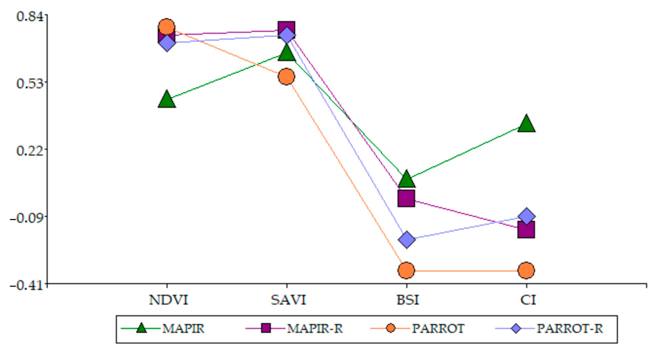
3.5. Relationship Between Sensors

Figure 11 presents a graph constructed from the averages of all the indices and cuts for each of the sensors used in the research. The above results demonstrate that there are marked differences between the spectral indices obtained and the remote sensors regarding their interaction with respect to the cut, while in a combined manner for NDVI, there is still a concordance between the Parrot and spectroradiometer sensors, while for Mapir, the values are well below the previous ones. For SAVI, there is a similarity between all the sensors, but SAVI values from the spectroradiometer present the greatest similarity. For BSI and CI, they present an equal tendency in the Parrot and spectroradiometer results, the unlike Mapir results, which present positive values outside the range of these soil indices.

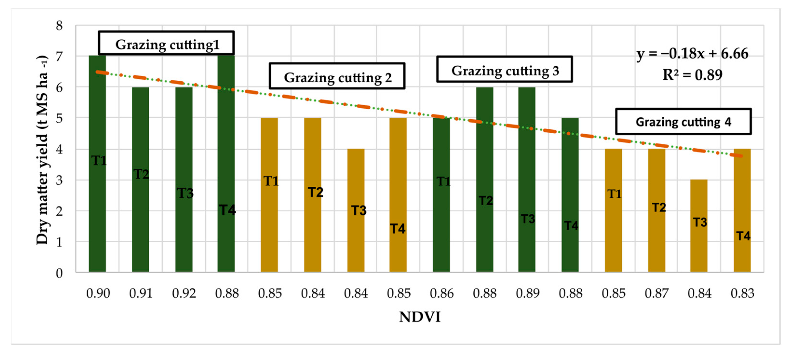
3.6. Sensor Validation and Yield and Botanical Composition Estimation

We performed a detailed intercorrelation analysis in order to explore the relationships between vegetation indices (NDVI, SAVI, BSI and CI) calculated from the three sensors evaluated in our study (PSR-1100 spectroradiometer, MAPIR and Parrot), which revealed significant associations between them. Since most of the index data failed to indicate a normal distribution according to the Shapiro–Wilk test (p < 0.05), we performed a Spearman correlation analysis, the results of which are presented further below.

To assess the internal consistency and reliability of the vegetation indices obtained using the modified MAPIR camera versus the spectroradiometer pseudo-bands, a Spearman correlation analysis was performed (Figure 12 and Figure 13). The strongest association was observed for SAVI (ρ = 0.67, p < 0.001), followed by NDVI (ρ = 0.59, p < 0.001), indicating moderate to strong agreement between these indices derived from both sensors. On the other hand, BSI yielded a moderate correlation (ρ = 0.46, p = 0.009), while CI presented a negative correlation of similar magnitude (ρ = 0.43, p = 0.014). These results suggest that SAVI and NDVI are the most robust indices when comparing MAPIR camera measurements with those from the spectroradiometer (Figure 12).

To evaluate the intercorrelation between vegetation indices obtained with the PARROT multispectral camera and the spectroradiometer indices, a Spearman correlation analysis was performed. The resulting graphs (Figure 12 and Figure 13) indicate strong positive associations for SAVI (ρ = 0.83, p < 0.001), NDVI (ρ = 0.79, p < 0.001) and CI (ρ = 0.78, p < 0.001), while the BSI yielded a moderate correlation (ρ = 0.46, p = 0.009). These results suggest that SAVI and NDVI derived from the PARROT camera are the indices that present the greatest consistency with the reference spectroradiometer measurements, supporting their use as robust indices for this type of assessment. This comparative analysis reinforces the reliability of the indices in monitoring forage cover vigor (Figure 13).

The Parrot results consistently demonstrated higher correlations than those of the MAPIR sensor for NDVI (ρ = 0.79 vs. 0.59), SAVI (ρ = 0.83 vs. 0.67) and CI (ρ = 0.78 vs. −0.43). For BSI, both sensors yielded similar correlations (ρ ≈ 0.46), with no clear advantage. For CI, the behavior was opposite between sensors, with PARROT measurements indicating a strong positive correlation (ρ = 0.78), while MAPIR results had a moderate negative correlation (ρ = −0.43), suggesting differences in spectral sensitivity or in the way the instruments respond to reflectance (Figure 14).

Finally, the NDVI values were closely correlated with forage yield proportions (R² = 0.8948), as demonstrated in Figure 15. The linear model expresses the direct relationship between yield and NDVI; i.e., if NDVI increases, the yield value will also increase.

On the other hand, in Figure 16, the relationship between NDVI values obtained from both sensors and the botanical composition is compared.

This set of scatter plots demonstrates the relationship between NDVI indices obtained from MAPIR, Parrot and spectroradiometer sensors as well as the botanical composition expressed as the percentage of perennial ryegrass and white clover in a forage mixture. No strong linear trends are evident, given the low coefficients of determination (R²) (less than 0.02), indicating that variation in the NDVI explains very little of the variation in the botanical composition.

In the case of NDVI_MAPIR, a negative slope is observed for perennial ryegrass and a positive slope for white clover, suggesting that for this sensor, an increase in NDVI was marginally associated with a lower percentage of ryegrass and a higher percentage of white clover. However, the R² was only 0.017, which prevents this relationship from being considered relevant from a predictive point of view. For NDVI_Parrot, the opposite is true. Here, slightly positive slopes are observed for perennial ryegrass and negative slopes for white clover, but also with an R² lower than 0.01. The calculated indices (MAPIR-R and Parrot-R) present practically flat lines, confirming the absence of a linear relationship.

4. Discussion

4.1. Performance Comparison

The absence of significant differences between treatments suggests that all grass–legume associations performed similarly in terms of total forage yield. However, the significant variation between cuts highlights the influence of seasonal conditions on productivity. As reported in previous studies [76,77], forage yields in perennial ryegrass- and clover-based pastures are strongly influenced by climatic seasonality, with higher yields typically observed during the rainy season (5–6 t DM ha⁻¹) and lower yields during the dry season (2–3 t DM ha⁻¹). These patterns are also affected by grazing management factors such as rest periods, paddock rotation and stocking rate.

The dominance of perennial ryegrass across all associations is consistent with its known competitive growth and adaptability to temperate Andean environments. Its contribution remained above 50% in all treatments, particularly during the rainy season, when favorable conditions promote rapid growth. In contrast, white clover showed lower overall productivity, though its contribution increased with higher sowing proportions. The higher yields observed in the 70:30 association confirm that under optimal light and moisture conditions, white clover can significantly contribute to total biomass, as previously reported for both annual and perennial clovers [85,86].

4.2. Vegetation Index Behavior

The NDVI results clearly show greater vegetation vigor before grazing (cuts 1, 3, 5 and 7), which aligns with previous findings where NDVI values of 0.94 and 0.87 were reported for perennial ryegrass using the Parrot Sequoia multispectral camera and the FieldSpec 4 spectroradiometer, respectively [26]. The lower NDVI values observed after grazing (cuts 2, 4, 6 and 8) reflect reduced vegetation vigor, consistent with the typical growth pattern of grass and its relationship with NDVI [87,88].

Regarding sensor performance, the Parrot and Parrot-R sensors recorded the highest NDVI values, while the Mapir sensor consistently showed significantly lower values. These differences may be attributed to technical characteristics such as spectral resolution and data acquisition height, as previously reported in studies comparing crop sensors and UAVs [89,90].

For the SAVI index, the highest values were also observed in pre-grazing cuts, particularly with the Mapir-R and Parrot-R sensors, indicating greater vegetation cover. The lowest values, recorded by the Parrot sensor in post-grazing cuts, correspond to areas with sparse vegetation or bare soil. This pattern is consistent with findings in kikuyu grass, where low SAVI values were associated with sparse vegetation and high values with dense vegetation [90,91,92].

Moreover, the substantial differences between spectroradiometers and spectral cameras may be due to variations in the field of view or data collection height. Such discrepancies have been documented in studies comparing different sensor types, where SAVI values varied significantly between crop sensors and UAVs [93,94].

4.3. Soil Index Behavior and Index Comparison

The BSI results for the Mapir sensor demonstrated no significant variation between pre- and post-grazing cuts, with all values remaining positive and relatively stable. This contrasts with the expected behavior of the BSI, which typically ranges from −1 to 1, where negative values indicate vegetated areas and positive values indicate bare soil [94]. The lack of differentiation in BSI values across grazing stages suggests that the Mapir sensor may not effectively capture soil exposure dynamics in this context.

In contrast, the Parrot sensor exhibited a clearer distinction between pre- and post-grazing cuts, with more negative BSI values in pre-grazing stages, indicating greater vegetation cover. These findings align with previous studies that explored the relationship between soil chemical properties and soil indices using spectroscopy [87].

Regarding the CI index, the Mapir sensor consistently recorded the highest values, while the Parrot sensor showed the lowest negative values during pre-grazing cuts. This pattern is consistent with earlier reports that associated negative CI values with higher vegetation presence [87]. The consistent performance of the Mapir sensor across all cuts may reflect its sensitivity to color variations in the soil–vegetation interface, although its tendency to produce higher values may also suggest overestimation in certain conditions.

The comparative analysis of vegetation and soil indices confirms that NDVI and SAVI are reliable indicators of vegetation vigor, particularly in distinguishing between pre- and post-grazing stages. Their parallel behavior across cuts reinforces their utility in monitoring pasture development. In contrast, BSI and CI, while useful for assessing soil exposure, showed greater variability depending on the sensor used. The Parrot and spectroradiometer sensors provided more consistent and interpretable results, especially in detecting changes in soil cover. The Mapir sensor, however, tended to produce higher and sometimes inconsistent values, particularly for BSI and CI, which may be attributed to differences in sensor calibration, field of view or data acquisition height.

These findings highlight the importance of sensor selection when interpreting spectral indices, as sensor characteristics can significantly influence the accuracy and reliability of vegetation and soil assessments.

4.4. Yield and Botanical Composition Estimation with Indices

The correlation analysis confirms that NDVI and SAVI are the most reliable vegetation indices for estimating forage vigor and yield, particularly when derived from the PARROT multispectral camera. The strong positive correlations observed between these indices and the spectroradiometer reference values (ρ > 0.79 for NDVI and ρ > 0.83 for SAVI) validate their robustness and suitability for remote sensing applications in pasture monitoring.

In contrast, the MAPIR camera showed lower correlations across all indices, especially for CI, where it exhibited a negative correlation (ρ = −0.43), suggesting potential limitations in its spectral sensitivity or calibration. The moderate correlation for BSI between both sensors (ρ ≈ 0.46) indicates that this index may be less reliable for distinguishing soil exposure in this context, possibly due to its sensitivity to background reflectance and sensor-specific characteristics.

The strong linear relationship between NDVI and forage yield (R² = 0.8948) further supports the use of NDVI as a predictive tool for biomass estimation. This finding is consistent with previous studies [87,95,96,97], which demonstrated the effectiveness of NDVI in estimating pasture yield by capturing vegetation spectral responses while minimizing soil background interference [46,48].

These results reinforce the value of NDVI and SAVI as key indicators for yield estimation and pasture management, particularly when using high-quality multispectral sensors such as the PARROT camera. On the other hand, the results of the correlation analysis between botanical composition and NDVI suggest that under the conditions of the present experiment and with the forage mixture evaluated, NDVI indices derived from multispectral and RGN sensors are not sufficient on their own to predict the botanical composition of grasses and legumes.

5. Conclusions

(1)

Yield estimation and species contribution

The forage mixture showed consistent yield across treatments, with the highest productivity observed during the first and second cuts in the rainy season (6.47 and 5.49 t DM ha⁻¹, respectively), contributing to a total yield of 20.46 t DM ha⁻¹. Perennial ryegrass was the dominant species, accounting for over 50% of the total yield (18.12 t DM ha⁻¹), while white clover contributed 3.10 t DM ha⁻¹. All proportions were optimal to obtain the highest grass yield in a forage mixture.

(2)

Spectral index behavior and sensor performance

Although no significant differences were found between treatments in vegetation and soil indices, significant interactions were observed between cuts and sensors. NDVI and SAVI values were consistently higher in pre-grazing cuts, reflecting greater biomass and canopy cover. Soil indices (BSI and CI) showed negative values, with BSI demonstrating better discrimination of bare soil due to its narrower value range. Thus, an increase in the indices was observed in the pre-grazing samplings, unlike the low values obtained for post-grazing.

(3)

Sensor comparison, correlation analysis and spectral limitations

The comparison between UAV-based sensors and the spectroradiometer revealed that the MAPIR RGN camera, despite its spectral limitations, produced acceptable correlation values with the spectroradiometer for vegetation indices—specifically NDVI and SAVI—with coefficients of 0.59 and 0.67, respectively. However, it showed poor performance for soil indices, likely due to its limited spectral range, non-standard band configuration and the low resolution of the modified lens. In contrast, the Parrot Sequoia camera showed generally consistent results across most indices but yielded a low correlation (0.46) for the chlorophyll index (CI), suggesting that this index should be excluded when using this sensor. These findings highlight the importance of sensor selection based on the specific indices and applications intended.

(4)

Importance of NDVI for yield prediction

NDVI was confirmed as a reliable indicator for predicting forage yield in mixed pastures of perennial ryegrass and white clover, aligning with previous studies. Its sensitivity to chlorophyll content and canopy structure makes it a valuable tool for monitoring crop development and productivity over time.

(5)

Practical implications

The integration of UAV-based remote sensing and field spectroscopy proved to be an efficient, non-invasive method for monitoring pasture growth. These technologies offer practical advantages for precision agriculture, enabling timely decision-making without the need for destructive sampling. Importantly, the evaluation of low-cost sensors such as the MAPIR camera provides valuable insights into their limitations and potential. Understanding how far these tools can reliably support vegetation monitoring is essential for guiding their use in developing regions or among farmers with limited resources, where access to high-end equipment may not be feasible.

(6)

Limitations and future research

This study was limited by the spectral resolution of some sensors and the temporal scope of data collection. Additionally, the research was conducted in a single study area, which restricts the ability to compare results across different edaphoclimatic conditions. This limits the generalizability of the findings to other regions with varying soil types, climates and management practices. Future research should consider multi-site studies across diverse agroecological zones, the integration of hyperspectral data and the application of machine learning techniques to enhance the robustness and scalability of remote sensing-based yield prediction models.

References

1. Vandehaar, M.J. Efficiency of nutrient use and relationship to profitability on dairy farms. J. Dairy Sci. 1998, 81, 272–282. [Google Scholar] [CrossRef] [PubMed]
2. Rotz, C.A.; Satter, L.D.; Mertens, D.R.; Muck, R.E. Feeding strategy, nitrogen cycling, and profitability of dairy farms. J. Dairy Sci. 1999, 82, 2841–2855. [Google Scholar] [CrossRef] [PubMed]
3. Tey, Y.S.; Brindal, M. Factors influencing farm profitability. Sustain. Agric. Rev. 2015, 15, 235–255. [Google Scholar]
4. Hanrahan, L.; McHugh, N.; Hennessy, T.; Moran, B.; Kearney, R.; Wallace, M.; Shalloo, L. Factors associated with profitability in pasture-based systems of milk production. J. Dairy Sci. 2018, 101, 5474–5485. [Google Scholar] [CrossRef]
5. Balehegn, M.; Duncan, A.; Tolera, A.; Ayantunde, A.A.; Issa, S.; Karimou, M.; Adesogan, A.T. Improving adoption of technologies and interventions for increasing supply of quality livestock feed in low-and middle-income countries. Glob. Food Secur. 2020, 26, 100372. [Google Scholar] [CrossRef]
6. Torres, B.; Cayambe, J.; Paz, S.; Ayerve, K.; Heredia-R, M.; Torres, E.; García, A. Livelihood capitals, income inequality, and the perception of climate change: A case study of small-scale cattle farmers in the Ecuadorian Andes. Sustainability 2022, 14, 5028. [Google Scholar] [CrossRef]
7. Wachendorf, C.; Stuelpnagel, R.; Wachendorf, M. Influence of land use and tillage depth on dynamics of soil microbial properties, soil carbon fractions and crop yield after conversion of short-rotation coppices. Soil. Use Manag. 2017, 33, 379–388. [Google Scholar] [CrossRef]
8. Wachendorf, M.; Fricke, T.; Möckel, T. Remote sensing as a tool to assess botanical composition, structure, quantity and quality of temperate grasslands. Grass Forage Sci. 2018, 73, 1–14. [Google Scholar] [CrossRef]
9. Cope, J.S.; Corney, D.; Clark, J.Y.; Remagnino, P.; Wilkin, P. Plant species identification using digital morphometrics: A review. Expert Syst. Appl. 2012, 39, 7562–7573. [Google Scholar] [CrossRef]
10. Heberling, J.M. Herbaria as big data sources of plant traits. Int. J. Plant Sci. 2022, 183, 87–118. [Google Scholar] [CrossRef]
11. Monteiro, A.; Santos, S.; Gonçalves, P. Precision agriculture for crop and livestock farming—Brief review. Animals 2021, 11, 2345. [Google Scholar] [CrossRef]
12. Sishodia, R.P.; Ray, R.L.; Singh, S.K. Applications of remote sensing in precision agriculture: A review. Remote Sens. 2020, 12, 3136. [Google Scholar] [CrossRef]
13. Liaghat, S.; Balasundram, S.K. A review: The role of remote sensing in precision agriculture. Am. J. Agric. Biol. Sci. 2010, 5, 50–55. [Google Scholar] [CrossRef]
14. Sabir, R.M.; Mehmood, K.; Sarwar, A.; Safdar, M.; Muhammad, N.E.; Gul, N.; Akram, H.M.B. Remote Sensing and Precision Agriculture: A Sustainable Future. In Transforming Agricultural Management for a Sustainable Future: Climate Change and Machine Learning Perspectives; Springer Nature: Cham, Switzerland, 2024; pp. 75–103. [Google Scholar]
15. Seelan, S.K.; Laguette, S.; Casady, G.M.; Seielstad, G.A. Remote sensing applications for precision agriculture: A learning community approach. Remote Sens. Environ. 2003, 88, 157–169. [Google Scholar] [CrossRef]
16. Aquilani, C.; Confessore, A.; Bozzi, R.; Sirtori, F.; Pugliese, C. Precision Livestock Farming technologies in pasture-based livestock systems. Animal 2022, 16, 100429. [Google Scholar] [CrossRef]
17. Shanmugapriya, P.; Rathika, S.; Ramesh, T.; Janaki, P. Applications of remote sensing in agriculture—A Review. Int. J. Curr. Microbiol. Appl. Sci. 2019, 8, 2270–2283. [Google Scholar] [CrossRef]
18. Wu, H.; Li, Z.L. Scale issues in remote sensing: A review on analysis, processing and modeling. Sensors 2009, 9, 1768–1793. [Google Scholar] [CrossRef]
19. Chi, M.; Plaza, A.; Benediktsson, J.A.; Sun, Z.; Shen, J.; Zhu, Y. Big data for remote sensing: Challenges and opportunities. Proc. IEEE 2016, 104, 2207–2219. [Google Scholar] [CrossRef]
20. Liu, P. A survey of remote-sensing big data. Front. Environ. Sci. 2015, 3, 45. [Google Scholar] [CrossRef]
21. Ali, I.; Cawkwell, F.; Dwyer, E.; Barrett, B.; Green, S. Satellite remote sensing of grasslands: From observation to management. J. Plant Ecol. 2016, 9, 649–671. [Google Scholar] [CrossRef]
22. Bégué, A.; Arvor, D.; Bellon, B.; Betbeder, J.; De Abelleyra, D.; PD Ferraz, R.; Verón, S.R. Remote sensing and cropping practices: A review. Remote Sens. 2018, 10, 99. [Google Scholar] [CrossRef]
23. Reinermann, S.; Asam, S.; Kuenzer, C. Remote sensing of grassland production and management—A review. Remote Sens. 2020, 12, 1949. [Google Scholar] [CrossRef]
24. Subhashree, S.N.; Igathinathane, C.; Akyuz, A.; Borhan, M.; Hendrickson, J.; Archer, D.; Halvorson, J. Tools for predicting forage growth in rangelands and economic analyses—A systematic review. Agriculture 2023, 13, 455. [Google Scholar] [CrossRef]
25. Pinter, P.J., Jr.; Hatfield, J.L.; Schepers, J.S.; Barnes, E.M.; Moran, M.S.; Daughtry, C.S.; Upchurch, D.R. Remote sensing for crop management. Photogramm. Eng. Remote Sens. 2003, 69, 647–664. [Google Scholar] [CrossRef]
26. Cevallos, L.N.M.; García, J.L.R.; Suárez, B.I.A.; González, C.A.L.; González, I.S.; Campoverde, J.A.Y.; Toulkeridis, T. A NDVI analysis contrasting different spectrum data methodologies applied in pasture crops previous grazing—A case study from Ecuador. In Proceedings of the 2018 International Conference on eDemocracy & eGovernment (ICEDEG), Ambato, Ecuador, 4–6 April 2018; IEEE: New York, NY, USA, 2018; pp. 126–135. [Google Scholar]
27. Curatola Fernández, G.F.; Obermeier, W.A.; Gerique, A.; Lopez Sandoval, M.F.; Lehnert, L.W.; Thies, B.; Bendix, J. Land cover change in the Andes of Southern Ecuador—Patterns and drivers. Remote Sens. 2015, 7, 2509–2542. [Google Scholar] [CrossRef]
28. García, V.J.; Márquez, C.O.; Rodríguez, M.V.; Orozco, J.J.; Aguilar, C.D.; Ríos, A.C. Páramo ecosystems in Ecuador’s southern region: Conservation state and restoration. Agronomy 2020, 10, 1922. [Google Scholar] [CrossRef]
29. Sönmez, N.; Emekli, Y.; Sari, M.; Baştuğ, R. Relationship between spectral reflectance water stress conditions of Bermuda grass. N. Z. J. Agric. Res. 2010, 51, 223. [Google Scholar] [CrossRef]
30. Jiang, Y.; Carrow, R.N. Broadband spectral reflectance models of turfgrass species and cultivars to drought stress. Crop Sci. 2007, 47, 1611–1618. [Google Scholar] [CrossRef]
31. Radoglou-Grammatikis, P.; Sarigiannidis, P.; Lagkas, T.; Moscholios, I. A compilation of UAV applications for precision agriculture. Comput. Netw. 2020, 172, 107148. [Google Scholar] [CrossRef]
32. Tsouros, D.C.; Bibi, S.; Sarigiannidis, P.G. A review on UAV-based applications for precision agriculture. Information 2019, 10, 349. [Google Scholar] [CrossRef]
33. Velusamy, P.; Rajendran, S.; Mahendran, R.K.; Naseer, S.; Shafiq, M.; Choi, J.G. Unmanned Aerial Vehicles (UAV) in precision agriculture: Applications and challenges. Energies 2021, 15, 217. [Google Scholar] [CrossRef]
34. Primicerio, J.; Di Gennaro, S.F.; Fiorillo, E.; Genesio, L.; Lugato, E.; Matese, A.; Vaccari, F.P. A flexible unmanned aerial vehicle for precision agriculture. Precis. Agric. 2012, 13, 517–523. [Google Scholar] [CrossRef]
35. Messina, G.; Modica, G. Applications of UAV thermal imagery in precision agriculture: State of the art and future research outlook. Remote Sens. 2020, 12, 1491. [Google Scholar] [CrossRef]
36. Srivastava, K.; Bhutoria, A.J.; Sharma, J.K.; Sinha, A.; Pandey, P.C. UAVs technology for the development of GUI based application for precision agriculture and environmental research. Remote Sens. Appl. Soc. Environ. 2019, 16, 100258. [Google Scholar] [CrossRef]
37. Sani, J.; Tierra, A.; Toulkeridis, T.; Padilla, O. Evaluation of Horizontal and Vertical Positions Obtained from an Unmanned Aircraft Vehicle Applied to Large Scale Cartography of Infrastructure Loss Due to the Earthquake of April 2016 in Ecuador. In International Conference on Applied Technologies; Springer Nature: Cham, Switzerland, 2022; pp. 60–73. [Google Scholar]
38. Shakhatreh, H.; Sawalmeh, A.H.; Al-Fuqaha, A.; Dou, Z.; Almaita, E.; Khalil, I.; Guizani, M. Unmanned aerial vehicles (UAVs): A survey on civil applications and key research challenges. IEEE Access 2019, 7, 48572–48634. [Google Scholar] [CrossRef]
39. Mohsan, S.A.H.; Khan, M.A.; Noor, F.; Ullah, I.; Alsharif, M.H. Towards the unmanned aerial vehicles (UAVs): A comprehensive review. Drones 2022, 6, 147. [Google Scholar] [CrossRef]
40. Pajares, G. Overview and current status of remote sensing applications based on unmanned aerial vehicles (UAVs). Photogramm. Eng. Remote Sens. 2015, 81, 281–330. [Google Scholar] [CrossRef]
41. Asadzadeh, S.; de Oliveira, W.J.; de Souza Filho, C.R. UAV-based remote sensing for the petroleum industry and environmental monitoring: State-of-the-art and perspectives. J. Pet. Sci. Eng. 2022, 208, 109633. [Google Scholar] [CrossRef]
42. Yao, H.; Qin, R.; Chen, X. Unmanned aerial vehicle for remote sensing applications—A review. Remote Sens. 2019, 11, 1443. [Google Scholar] [CrossRef]
43. O’Connor, J.; Smith, M.J.; James, M.R. Cameras and settings for aerial surveys in the geosciences: Optimising image data. Prog. Progress. Phys. Geogr. 2017, 41, 325–344. [Google Scholar] [CrossRef]
44. Yang, Z.; Yu, X.; Dedman, S.; Rosso, M.; Zhu, J.; Yang, J.; Wang, J. UAV remote sensing applications in marine monitoring: Knowledge visualization and review. Sci. Total Environ. 2022, 838, 155939. [Google Scholar] [CrossRef]
45. Xue, J.; Su, B. Significant remote sensing vegetation indices: A review of developments and applications. J. Sens. 2017, 2017, 1353691. [Google Scholar] [CrossRef]
46. Bannari, A.; Morin, D.; Bonn, F.; Huete, A. A review of vegetation indices. Remote Sens. Rev. 1995, 13, 95–120. [Google Scholar] [CrossRef]
47. Rondeaux, G.; Steven, M.; Baret, F. Optimization of soil-adjusted vegetation indices. Remote Sens. Environ. 1996, 55, 95–107. [Google Scholar] [CrossRef]
48. Glenn, E.P.; Huete, A.R.; Nagler, P.L.; Nelson, S.G. Relationship between remotely-sensed vegetation indices, canopy attributes and plant physiological processes: What vegetation indices can and cannot tell us about the landscape. Sensors 2008, 8, 2136–2160. [Google Scholar] [CrossRef] [PubMed]
49. Huete, A.R. Vegetation indices, remote sensing and forest monitoring. Geogr. Compass 2012, 6, 513–532. [Google Scholar] [CrossRef]
50. Qi, J.; Chehbouni, A.; Huete, A.R.; Kerr, Y.H.; Sorooshian, S. A modified soil adjusted vegetation index. Remote Sens. Environ. 1994, 48, 119–126. [Google Scholar] [CrossRef]
51. Rosell, J.R.; Sanz, R. A review of methods and applications of the geometric characterization of tree crops in agricultural activities. Comput. Electron. Agric. 2012, 81, 124–141. [Google Scholar] [CrossRef]
52. Lee, W.S.; Alchanatis, V.; Yang, C.; Hirafuji, M.; Moshou, D.; Li, C. Sensing technologies for precision specialty crop production. Comput. Electron. Agric. 2010, 74, 2–33. [Google Scholar] [CrossRef]
53. Chlingaryan, A.; Sukkarieh, S.; Whelan, B. Machine learning approaches for crop yield prediction and nitrogen status estimation in precision agriculture: A review. Comput. Electron. Agric. 2018, 151, 61–69. [Google Scholar] [CrossRef]
54. Yengoh, G.T.; Dent, D.; Olsson, L.; Tengberg, A.E.; Tucker, C.J., III. Use of the Normalized Difference Vegetation Index (NDVI) to Assess Land Degradation at Multiple Scales: Current Status, Future Trends, and Practical Considerations; Springer: Berlin/Heidelberg, Germany, 2015. [Google Scholar]
55. Adar, S.; Sternberg, M.; Argaman, E.; Henkin, Z.; Dovrat, G.; Zaady, E.; Paz-Kagan, T. Testing a novel pasture quality index using remote sensing tools in semiarid and Mediterranean grasslands. Agric. Ecosyst. Environ. 2023, 357, 108674. [Google Scholar] [CrossRef]
56. Oliveira, R.A.; Näsi, R.; Korhonen, P.; Mustonen, A.; Niemeläinen, O.; Koivumäki, N.; Honkavaara, E. High-precision estimation of grass quality and quantity using UAS-based VNIR and SWIR hyperspectral cameras and machine learning. Precis. Agric. 2024, 25, 186–220. [Google Scholar] [CrossRef]
57. Nicola, F.; Miguel, R.C.J.; Intrigliolo, D.S.; Giuseppe, T.; Sabina, F. Remote Sensing for Pasture Biomass Quantity and Quality Assessment: Challenges and Future Prospects. Smart Agric. Technol. 2025, 12, 101057. [Google Scholar] [CrossRef]
58. Shahi, T.B.; Balasubramaniam, T.; Sabir, K.; Nayak, R. Pasture monitoring using remote sensing and machine learning: A review of methods and applications. Remote Sens. Appl. Soc. Environ. 2025, 37, 101459. [Google Scholar] [CrossRef]
59. Shorten, P.R.; Trolove, M.R. UAV-based prediction of ryegrass dry matter yield. Int. J. Remote Sens. 2022, 43, 2393–2409. [Google Scholar] [CrossRef]
60. De Rosa, D.; Basso, B.; Fasiolo, M.; Friedl, J.; Fulkerson, B.; Grace, P.R.; Rowlings, D.W. Predicting pasture biomass using a statistical model and machine learning algorithm implemented with remotely sensed imagery. Comput. Electron. Agric. 2021, 180, 105880. [Google Scholar] [CrossRef]
61. Freitas, R.G.; Pereira, F.R.; Dos Reis, A.A.; Magalhães, P.S.; Figueiredo, G.K.; do Amaral, L.R. Estimating pasture aboveground biomass under an integrated crop-livestock system based on spectral and texture measures derived from UAV images. Comput. Electron. Agric. 2022, 198, 107122. [Google Scholar] [CrossRef]
62. Pranga, J.; Borra-Serrano, I.; Aper, J.; De Swaef, T.; Ghesquiere, A.; Quataert, P.; Lootens, P. Improving accuracy of herbage yield predictions in perennial ryegrass with UAV-based structural and spectral data fusion and machine learning. Remote Sens. 2021, 13, 3459. [Google Scholar] [CrossRef]
63. Sinde-González, I.; Gil-Docampo, M.; Arza-García, M.; Grefa-Sánchez, J.; Yánez-Simba, D.; Pérez-Guerrero, P.; Abril-Porras, V. Biomass estimation of pasture plots with multitemporal UAV-based photogrammetric surveys. Int. J. Appl. Earth Obs. Geoinf. 2021, 101, 102355. [Google Scholar] [CrossRef]
64. Fernandez-Figueroa, E.G.; Wilson, A.E.; Rogers, S.R. Commercially available unoccupied aerial systems for monitoring harmful algal blooms: A comparative study. Limnol. Oceanogr. Methods 2022, 20, 146–158. [Google Scholar] [CrossRef]
65. Hall, M.L.; Samaniego, P.; Le Pennec, J.L.; Johnson, J.B. Ecuadorian Andes volcanism: A review of Late Pliocene to present activity. J. Volcanol. Geotherm. Res. 2008, 176, 1–6. [Google Scholar] [CrossRef]
66. Toulkeridis, T.; Zach, I. Wind directions of volcanic ash-charged clouds in Ecuador–implications for the public and flight safety. Geomat. Nat. Hazards Risk 2017, 8, 242–256. [Google Scholar] [CrossRef]
67. INAMHI Instituto Nacional de Meteorología e Hidrología. Estadística Climatológica. Datos Meteorológicos Correspondientes al Periodo Enero–Diciembre 2019; Estación Izobamba: Mejía, Ecuador, 2019. [Google Scholar]
68. Burdon, J.J. Trifolium repens L. J. Ecol. 1983, 71, 307–330. [Google Scholar] [CrossRef]
69. Turkington, R.; Harper, J.L. The growth, distribution and neighbour relationships of Trifolium repens in a permanent pasture: IV. Fine-scale biotic differentiation. J. Ecol. 1979, 67, 245–254. [Google Scholar] [CrossRef]
70. Vásquez, H.V.; Valqui, L.; Bobadilla, L.G.; Meseth, E.; Trigoso, M.J.; Zagaceta, L.H.; Maicelo, J.L. Agronomic and Nutritional Evaluation of INIA 910—Kumymarca Ryegrass (Lolium multiflorum Lam.): An Alternative for Sustainable Forage Production in Department of Amazonas (NW Peru). Agronomy 2025, 15, 100. [Google Scholar] [CrossRef]
71. Lee, J.M.; Matthew, C.; Thom, E.R.; Chapman, D.F. Perennial ryegrass breeding in New Zealand: A dairy industry perspective. Crop Pasture Sci. 2012, 63, 107–127. [Google Scholar] [CrossRef]
72. Annicchiarico, P.; Carelli, M. Origin of Ladino white clover as inferred from patterns of molecular and morphophysiological diversity. Crop Sci. 2014, 54, 2696–2706. [Google Scholar] [CrossRef]
73. Nicolau, S.T.; Matzger, A.J. An evaluation of resolution, accuracy, and precision in FT-IR spectroscopy. Spectrochim. Acta Part A Mol. Biomol. Spectrosc. 2024, 319, 124545. [Google Scholar] [CrossRef]
74. Akin, D.E.; Burdick, D. Percentage of Tissue Types in Tropical and Temperate Grass Leaf Blades and Degradation of Tissues by Rumen Microorganisms 1. Crop Sci. 1975, 15, 661–668. [Google Scholar] [CrossRef]
75. León, R.; Bonifaz, N.; Gutiérrez, F. Pastos Y Forrajes del Ecuador: Siembra Y Producción De pasturas, 3rd ed.; Editorial Universitaria Abya-Yala: Quito, Ecuador, 2018. [Google Scholar]
76. Muñoz, E.C.; Andriamandroso, A.L.H.; Beckers, Y.; Ron, L.; Montufar, C.; da Silva Neto, G.F.; Bindelle, J. Analysis of the nutritional and productive behaviour of dairy cows under three rotation bands of pastures, Pichincha, Ecuador. J. Agric. Rural Dev. Trop. Subtrop. 2021, 122, 289–298. [Google Scholar]
77. Velasco, L.; Condolo, L.; Vaca, M.; Santos, C. Nutritional Contribution of Cultivated Pastures in the Eastern Part of Ecuador. J. Surv. Fish. Sci. 2023, 1, 214–221. [Google Scholar]
78. Sanderson, M.A.; Soder, K.J.; Muller, L.D.; Klement, K.D.; Skinner, R.H.; Goslee, S.C. Forage mixture productivity and botanical composition in pastures grazed by dairy cattle. Agron. J. 2005, 97, 1465–1471. [Google Scholar] [CrossRef]
79. Trotter, M. PA Innovations in livestock, grazing systems and rangeland management to improve landscape productivity and sustainability. Agric. Sci. 2013, 25, 27–31. [Google Scholar]
80. INIAP. Laboratorio de Suelos Y Calidad Nutricional: Toma de Muestras Para Análisis de Suelos, Aguas Y Plantas; Instituto Nacional Autónomo de Investigaciones Agropecuarias (INIAP): Quito, Ecuador, 2018; p. 2. [Google Scholar]
81. Franzini, M.; Ronchetti, G.; Sona, G.; Casella, V. Geometric and radiometric consistency of parrot sequoia multispectral imagery for precision agriculture applications. Appl. Sci. 2019, 9, 5314. [Google Scholar] [CrossRef]
82. Moriarty, C.; Cowley, D.C.; Wade, T.; Nichol, C.J. Deploying multispectral remote sensing for multi-temporal analysis of archaeological crop stress at Ravenshall, Fife, Scotland. Archaeological Prospection 2019, 26, 33–46. [Google Scholar] [CrossRef]
83. MAPIR. Survey3W Camera—Red+Green+NIR (RGN, NDVI). MAPIR CAMERA. 2021. Available online: https://www.mapir.camera/products/survey3w-camera-red-green-nir-rgn-ndvi (accessed on 17 July 2025).
84. Reeves, M.; Fulkerson, W.J.; Kellaway, R.C. Forage quality of kikuyu (Pennisetum clandestinum): The effect of time of defoliation and nitrogen fertiliser application and in comparison with perennial ryegrass (Lolium perenne). Aust. J. Agric. Res. 1996, 47, 1349–1359. [Google Scholar] [CrossRef]
85. Pauly, K. Applying conventional vegetation vigor indices to UAS-derived orthomosaics: Issues and considerations. In Proceedings of the 12th International Conference for Precision Agriculture, Sacramento, CA, USA, 20–23 July 2014; pp. 20–23. [Google Scholar]
86. Escadafal, R. Remote sensing of arid soil surface color with Landsat thematic mapper. Adv. Space Res. 1989, 9, 159–163. [Google Scholar] [CrossRef]
87. Arciniegas-Ortega, S.; Molina, I.; Garcia-Aranda, C. Soil order-land use index using field-satellite spectroradiometry in the Ecuadorian Andean Territory for modeling soil quality. Sustainability 2022, 14, 7426. [Google Scholar] [CrossRef]
88. Castro, R.; Hernández, A.; Vaquera, H.; Hernández, J.; Quero, A.; Enríquez, J.; Martínez, P. Comportamiento productivo de asociaciones de gramíneas con leguminosas en pastoreo. Rev. Fitotec. Mex. 2012, 35, 87. [Google Scholar] [CrossRef]
89. Villalobos, L.; Sánchez, J. Evaluación agronómica y nutricional del pasto Rye grass Perenne Tetraploide (Lolium perenne) producido en lecherías de las zonas altas de Costa Rica. II. Valor nutricional. Agron. Costarric. 2016, 34, 43–52. [Google Scholar]
90. Dronova, I.; Taddeo, S. Remote sensing of phenology: Towards the comprehensive indicators of plant community dynamics from species to regional scales. J. Ecol. 2022, 110, 1460–1484. [Google Scholar] [CrossRef]
91. Hamada, Y.; Stow, D.A.; Roberts, D.A. Estimating life-form cover fractions in California sage scrub communities using multispectral remote sensing. Remote Sens. Environ. 2011, 115, 3056–3068. [Google Scholar] [CrossRef]
92. Ruiz, D.A.C.; Villacís, M.G.M.; Kirby, E.; Guzmán, J.A.M.; Toulkeridis, T. Correlation of NDVI obtained by different methodologies of spectral data collection in a commercial crop of Quinoa (Chenopodium Quinoa) in central Ecuador. In Proceedings of the 2020 Seventh International Conference on eDemocracy & eGovernment (ICEDEG), Buenos Aires, Argentina, 22–24 April 2020; IEEE: New York, NY, USA, 2020; pp. 208–215. [Google Scholar]
93. Villacís, M.G.M.; Ruiz, D.A.C.; Powney, E.P.K.; Guzmán, J.A.M.; Toulkeridis, T. Index relationship of vegetation with the development of a Quinoa Crop (Chenopodium quinoa) in its first phenological stages in central Ecuador based on GIS techniques. In Proceedings of the 2020 Seventh International Conference on eDemocracy & eGovernment (ICEDEG), Buenos Aires, Argentina, 22–24 April 2020; IEEE: New York, NY, USA, 2020; pp. 191–200. [Google Scholar]
94. Marais, J.P. Factors affecting the nutritive value of kikuyu grass (Pennisetum clandestinum)—A review. Trop. Grassl. 2001, 35, 65–84. [Google Scholar]
95. Kumar, P.; Pandey, P.; Singh, B.; Katiyar, S.; Mandal, V.; Rani, M.; Tomar, V.; Patairiya, S. Estimation of accumulated soil organic carbon stock in tropical forest using geospatial strategy. Egypt. J. Remote Sens. Space Sci. 2016, 19, 109–123. [Google Scholar] [CrossRef]
96. Sinde, I.; Yánez, D.; Grefa, J.; Arza, M.; Gil, M. Estimación del rendimiento del pasto mediante NDVI con imágenes multiespectrales de vehículos aéreos no tripulados (UAV). Rev. Geoespacial 2020, 17, 14. [Google Scholar]
97. Aper, J.; Borra-Serrano, I.; Ghesquiere, A.; De Swaef, T.; Roldán-Ruiz, I.; Lootens, P.; Baert, J. Yield estimation of perennial ryegrass plots in breeding trials using UAV images. In Improving Sown Grasslands Through Breeding and Management; Wageningen Academic Publishers: Wageningen, The Netherlands, 2019; pp. 312–314. [Google Scholar]
Figure 1. Flowchart of the applied methodology of the present study.
Remotesensing 17 02561 g001
Figure 2. Location of the study site and parcellation map.
Remotesensing 17 02561 g002
Figure 3. GCP control points obtained in SNAP Note. The eight points located in each EU were used to generate the pixel values of all the indices for both Parrot and Mapir cameras.
Remotesensing 17 02561 g003
Figure 4. Botanical composition by section of four grass and legume planting treatments.
Remotesensing 17 02561 g004
Figure 5. Images of the UAV vegetation indices.
Remotesensing 17 02561 g005
Figure 6. Result of the 5% Tukey test for NDVI and SAVI per cut and sensor.
Remotesensing 17 02561 g006
Figure 7. Images of the UAV soil indices.
Remotesensing 17 02561 g007
Figure 8. The 5% Tukey test results for BSI per cut for the Parrot sensor.
Remotesensing 17 02561 g008
Figure 9. The 5% Tukey test results for CI by cut for Parrot sensor.
Remotesensing 17 02561 g009
Figure 10. Vegetation and soil indices vs. cuts.
Remotesensing 17 02561 g010
Figure 11. Vegetation and soil indices vs. sensors.
Remotesensing 17 02561 g011
Figure 12. Relationships between vegetation indices obtained with the MAPIR camera and pseudo-bands of the spectroradiometer using Spearman correlation.
Remotesensing 17 02561 g012
Figure 13. Relationships between vegetation indices obtained with a multispectral camera (PARROT) and simulated bands of the spectroradiometer using Spearman correlation.
Remotesensing 17 02561 g013
Figure 14. Correlation (Spearman’s ρ) of indices between MAPIR and PARROT sensors. The graph compares the Spearman correlation coefficients (ρ) between the vegetation indices calculated with the MAPIR and PARROT cameras and the same indices generated from the spectroradiometer (pseudo-bands).
Remotesensing 17 02561 g014
Figure 15. NDVI vs. yield.
Remotesensing 17 02561 g015
Figure 16. Scatter plot of relationships between NDVI indices obtained from MAPIR and PARROT sensors and the botanical composition of perennial ryegrass and white clover.
Remotesensing 17 02561 g016