On the Usage of Deep Learning Techniques for Unmanned Aerial Vehicle-Based Citrus Crop Health Assessment

Abstract

This work proposes an end-to-end solution for leaf segmentation, disease detection, and damage quantification, specifically focusing on citrus crops. The primary motivation behind this research is to enable the early detection of phytosanitary problems, which directly impact the productivity and profitability of Spanish and Portuguese agricultural developments, while ensuring environmentally safe management practices. It integrates an onboard computing module for Unmanned Aerial Vehicles (UAVs) using a Raspberry Pi 4 with Global Positioning System (GPS) and camera modules, allowing the real-time geolocation of images in citrus croplands. To address the lack of public data, a comprehensive database was created and manually labelled at the pixel level to provide accurate training data for a deep learning approach. To reduce annotation effort, we developed a custom automation algorithm for pixel-wise labelling in complex natural backgrounds. A SegNet architecture with a Visual Geometry Group 16 (VGG16) backbone was trained for the semantic, pixel-wise segmentation of citrus foliage. The model was successfully integrated as a modular component within a broader system architecture and was tested with UAV-acquired images, demonstrating accurate disease detection and quantification, even under varied conditions. The developed system provides a robust tool for the efficient monitoring of citrus crops in precision agriculture.

1. Introduction

This work addresses the necessity for the early detection of phytosanitary problems, which directly influence the productivity and profitability of some Spanish and Portuguese farming developments. It aims to support sustainable decision-making in precision agriculture (PA) applications to minimise the environmental impact of current agricultural practices. Specifically, this involves protecting local flora and fauna, optimising the use of fertilisers or pesticides to reduce chemical pollutants, and rationalising the use of available resources [1]. Hence, the main motivation behind selecting this field of study was the desire to address problems that directly affect familiar agricultural land. To achieve this, available technology is used as a precise tool to enhance the efficiency of the development process, reducing the need for human effort and time-consuming tasks.

The importance of the agricultural sector for human development and the global economy cannot be denied. Nevertheless, the sensitivity of this field to unexpected events, such as climate change or phytosanitary problems, poses a great challenge that can lead to significant economic losses. To address these challenges, the scientific community is working on innovative strategies, including the use of drones for PA [2]. Drones offer versatility and efficiency in agricultural applications, such as reducing fertiliser waste and collecting high-resolution aerial images at a lower cost [3]. Despite the growing interest in this field, there is a lack of alternative studies using the methodology employed in this research for the detection of phytosanitary problems. The objective of this project is to develop and test a multidisciplinary engineering system integrated into a quadcopter for the timely detection of agricultural issues, data acquisition, and environmentally sustainable decision-making based on the damage threshold defined by integrated production.

1.1. Citrus Phytosanitary Problems

Citrus production is one of the most important economic agricultural activities in the world. According to the Food and Agriculture Organisation (FAO), 122 million tons of citrus fruits are produced annually [2]. However, economic losses in citrus production have increased the necessity for innovative strategies in this competitive sector, in which demand depends heavily on the phytosanitary state, which is usually beyond the control of farmers, as well as the availability of high-quality products [4].

Table 1. Huanglongbing disease and damage threshold according to integrated production.

Disease	Huanglongbing (Greening) Candidatus Liberibacter [2,5]
Symptoms	Leaf discolouration and yellow blotches
Diagnosis Methods	Visual inspection, DNA tests, Polymerase Chain Reaction (PCR)
Threshold	≥10% of leaves affected
Phenological stage	All year long

presents the citrus phytosanitary problem studied in this research, Huanglongbing (HLB), along with its corresponding damage threshold and the optimal time recommended by integrated production for pest management applications to effectively mitigate its effects. Integrated production is a sustainable mode of agricultural production that involves the rational application of farming and livestock techniques, employing appropriate agricultural practices at the correct intensity and time, in order to increase production quality and ensure sustainable agriculture [1]. Specifically, greening disease, compared to other phytosanitary issues, has fewer limitations concerning the optimal time or appropriate phenological stage for treatment application, enabling quicker actions by farmers to address the problem at any time of the year.

1.2. Application of UAVs in Precision Agriculture

Unmanned Aerial Vehicles (UAVs) have recently been utilised as a component in PA. According to [6], this entails “a whole-farm management concept based on observing, measuring and responding to inter- and intra-field variability in crops”, using current technology, remote sensing and satellite positioning data to increase the profitability of production for the farmer and develop “appropriate farming practices” [6]. UAVs have successfully increased agricultural productivity and farm economic and operating profits, while also reducing in-field walking costs and the need for observational experiments [3]. In this regard, UAVs facilitate weed monitoring, environmentally safe pest control and detection, agricultural management, and real-time information collection, among other tasks. In addition, they enable more accurate yield and health assessment and help address the lack of high-resolution aerial images compared with conventional techniques.

To date, there have been various applications of drones in this field, such as soil and field analysis, planting crops and trees, livestock management, geofencing and protection of fields from animal damage, and even crop spraying, which involves scanning the ground and applying the appropriate amount of chemicals based on crop conditions [7]. Apart from these applications, drones aid in weed identification and irrigation, which are crucial for economic development and water stress management. These capabilities ensure efficient irrigation and the application of remedial measures based on actual needs and prevent water and resource wastage [3,8]. In addition, drones assist in monitoring and assessing crop health, which is essential for monitoring field conditions and enabling the early detection of diseases. This reduces the need for visual inspection by farmers and supports the use of computer vision technology to provide timely information to farmers [7]. Thus, as mentioned previously, these applications represent the main purpose of this project. Indeed, in agriculture, the early detection of spot bacteria, fungal infections, and stress is vital for preventing crop yield losses [9]. For this reason, remote sensors are increasingly being utilised in PA to develop novel techniques for performing labour-intensive tasks and for monitoring and mapping crops in areas that are otherwise physically challenging to reach. According to [9], there are several sensors and methods used by farmers to detect biotic (disease) and abiotic (nutritional) stresses in plants.

Traditional manual field surveys based on visual disease assessment have limitations due to high subjectivity in diagnosis and delays in detection. To overcome these challenges, more precise methodologies have been developed, using a wide range of sensors, which can be classified as proximal sensors and remote sensing (RS) technologies [3].

1.3. Computer Vision Technologies for Smart Agriculture

According to Ragazou et al. [10], from 2017 to 2021, there has been a significant surge in scientific interest in the field of smart farming. This has resulted in the adoption of digital technologies in both crop and livestock agricultural production, which characterises the era of “smart farming”. Smart farming is a modernised and integrated production system that takes advantage of technological advancements and decision-making processes. Furthermore, it combines all factors of production and integrates agricultural research and knowledge to optimise the efficiency of the agricultural sector [10].

Computer vision (CV) applications are growing in contemporary agriculture [11], motivated by the potential of training deep neural networks. These networks learn multi-level representations of data, efficiently handle large volumes of information, and leverage parallel hardware architectures, such as Graphical Processing Units (GPUs). In smart agriculture, CV is used for image recognition, object detection, segmentation, and uncertainty quantification [12]. Consequently, various neural network technologies, such as ResNet [13], AlexNet [14,15], SegNet [16], and GoogLeNet [17], have been developed for the management of crops, livestock, and farms [11]. In addition, CV capabilities are applied to pest and disease detection [18], growth monitoring [17,19], fruit and flower detection [20,21], fruit counting [22], and maturity-level classification [11].

In particular, image segmentation refers to the process of classifying each pixel in an image into a specific object or object instance [11]. Specifically, in semantic segmentation, each object in an image is assigned to a specific class, with different instances of the same object sharing the same class label. In agriculture, image-based plant phenotyping, particularly leaf segmentation, has gained prominence [23]. Despite leaves sharing common visual and morphological attributes, challenges arise due to occlusions, variations in leaf shape and orientation, and imaging conditions. Consequently, traditional computer vision techniques [18,19,23], as well as artificial intelligence-based solutions, have been proposed. State-of-the-art neural network technologies, like Convolutional Neural Network (CNN) models [24], including the DenseNet and 1D CNN models [25], offer promising approaches for crop leaf and plant instance segmentation, disease classification, and damage detection. Additionally, the SegNet model has shown promising results in multiple tree leaf segmentation, weed detection, and panicle counting from UAV images [16,26,27]. Moreover, at the forefront of recent AI research, Meta AI’s Segment Anything Model (SAM) is capable of segmenting any object in any image “zero-shot” performance on unfamiliar objects [28].

Recent advances in deep learning have enabled new architectures that significantly improve the performance and efficiency of semantic segmentation tasks. One of the most widely adopted models is DeepLabv3+, which uses atrous separable convolutions and an encoder–decoder structure to enhance boundary delineation and multi-scale feature learning [29]. For real-time applications and embedded systems, lightweight models such as Fast-SCNN and BiSeNet have been proposed, offering a good trade-off between speed and accuracy [30,31]. In the context of agricultural image analysis, recent studies have explored UAV-based imaging for citrus crop monitoring, focusing on canopy-level segmentation and early disease detection. For example, in [32,33], methods for segmenting the citrus canopy were developed, while in [34], semantic segmentation was applied using multispectral UAV imagery to delineate the crowns of citrus trees. More recently, works such as [35,36] have addressed the early detection of citrus greening (HLB) using UAV-based multispectral imagery and deep learning. In particular, [36] proposed a modified U-Net model (MGA-U-Net) for pixel-wise classification of symptomatic trees. However, these studies generally operate at the tree or plot level and do not address the fine-grained segmentation of individual leaves or symptomatic regions within the canopy. In contrast, the present work proposes a novel pixel-level semantic segmentation approach focused on citrus foliage and disease symptoms at the leaf scale, acquired under real field conditions with a low-cost RGB UAV. It also introduces a semi-automated annotation strategy tailored for natural environments and an onboard image acquisition system compatible with autonomous flight. To the best of our knowledge, this is the first work to jointly address all these aspects—granularity, automation, and hardware feasibility—in the context of citrus disease detection.

1.4. Technical and Innovative Contributions of This Paper

This work proposes a complete and low-cost methodology for the early detection of citrus crop greening (HLB) disease by integrating a UAV-based image acquisition system with a deep learning model for semantic segmentation. The system is designed to operate under real outdoor conditions and provide actionable information for precision agriculture decision-making. The proposed solution includes the design and deployment of a customised data acquisition system, the generation of a novel dataset of citrus foliage images, the development of a pixel-level labelling algorithm as a proof of concept, and the training of deep neural networks for leaf segmentation. The final deep learning model replaces the shape recognition algorithm presented in our previous research [18], allowing accurate segmentation of new and unseen data. Disease recognition and damage quantification are carried out following the methodology described in [18].

The main technical and scientific contributions of this work are summarised as follows:

• Integration of a UAV-compatible onboard image acquisition system, based on the Raspberry Pi 4, equipped with camera and GPS modules, capable of collecting high-resolution, geolocated images of citrus foliage under real field conditions.
• Creation of a new dataset of citrus foliage images, captured in natural agricultural environments, reflecting real-world variability in lighting, background, leaf morphology, and disease stages—addressing the absence of suitable public datasets for this task.
• Development of a custom automation algorithm for semantic segmentation annotation, implemented in MATLAB’s “Image Labeler App”, which significantly reduces manual annotation time for complex natural images by leveraging pre-trained models.
• Design and training of deep learning models based on a SegNet encoder–decoder architecture with a VGG16 backbone for semantic, pixel-wise segmentation of citrus leaves. The final model replaces the shape recognition block of our previous work [18].
• Validation of the complete system using data acquired in UAV flight tests, demonstrating robustness, generalisation to unseen data, and suitability for real-time and real-world applications in smart agriculture.

These contributions offer a reliable and practical solution for precision agriculture and can be extended to other plant species and agricultural monitoring scenarios.

2. Materials and Methods

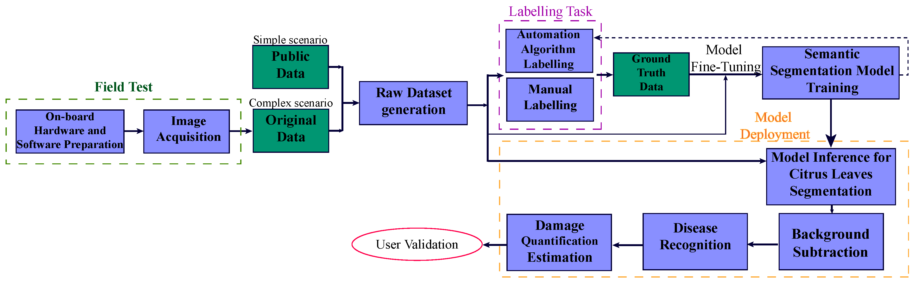
An overview of the final flowchart for the proposed image-based plant phenotyping detection methodology is shown in Figure 1 and presented in the following sections.

2.1. Hardware and Software Components for Photographic Data Acquisition and Geolocation Control

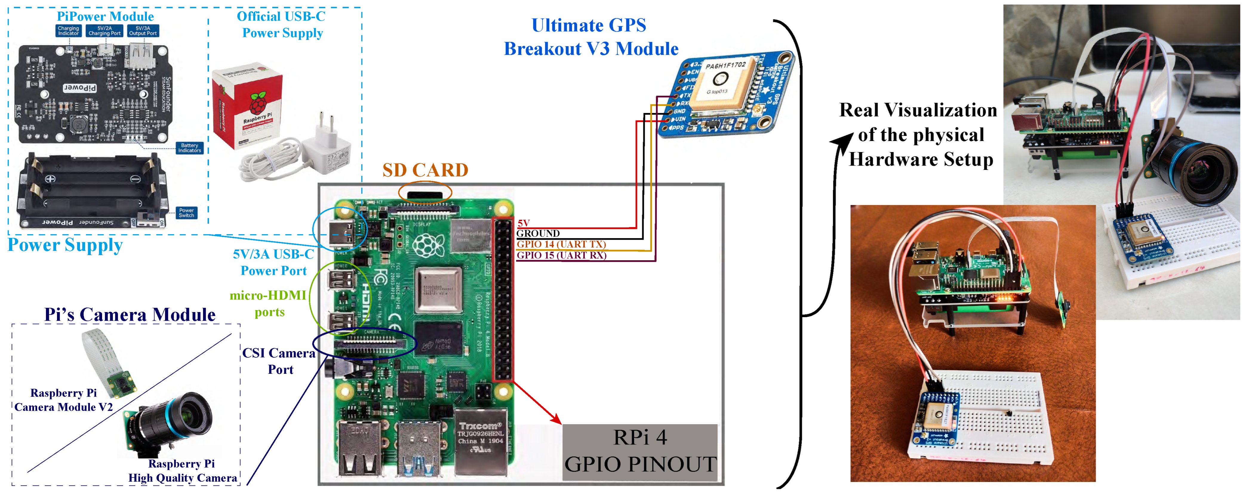
The hardware components of the onboard data acquisition control system are as follows:

• Raspberry Pi (RPi) 4 Model B—This single-board computer is used to interact with the Global Positioning System (GPS) module and video camera. It incorporates Wi-Fi 802.11ac for wireless connections. The Raspberry Pi operating system, along with all the data and images generated by the image acquisition and GPS, is stored on a 16 GB SD card permanently attached to the RPi board. In addition, the PiPower module is used as the power supply for the Raspberry Pi.
• Raspberry Pi camera module—This high-quality camera module is specifically designed for use with Raspberry Pi boards. It can be used to capture either high-definition videos or photographs. In this case, two different RPi camera modules were used to capture images of unhealthy citrus crops [37]:

  -

  Raspberry Pi camera module V2—This module includes an 8 MP Sony IMX219 image sensor capable of capturing 3280 × 2464-pixel still images, transferring data at high speeds, and adjusting image focus.

  -

  Raspberry Pi high-quality (HQ) camera module—This module includes a 12.3 MP Sony IMX477 sensor that captures high-resolution still images of 4056 × 3040 pixels. It also includes adjustable back focus and supports interchangeable lenses.

• Ultimate GPS Breakout V3 module—This module receives signals from GPS satellites through a GPS receiver to determine the fixed position on Earth, leaving open the possibility of future trajectory mapping.

Figure 2 shows a schematic representation of the hardware components and their interconnections in the system. The need to conduct field tests in a natural environment significantly influenced both the hardware and software configurations, as well as the proposed detection system scheme (detailed in Section 2.2). The scheme provides a visual overview of the system architecture, which is complemented by a real image of the setup on the right-hand side.

The data acquisition control system is a complex system that requires various programming languages and software programs, broadly categorised into those used for wireless communication between the data acquisition control system and the user interface, and those specific to operating hardware devices. Wireless communication is made possible through the Wi-Fi wireless module, which enables the use of the following software applications for graphical interface visualisation, as well as for remote access and control:

• VNC Viewer 6.22.515: This is RealVNC’s open software tool that allows remote access to and control of another computer in real time using the Remote Framebuffer (RFB) protocol.
• WinSCP: This is a Secure File Transfer Protocol (SFTP) client that enables secure file transfer between a local and a remote computer.

The Raspberry Pi executes a runtime developed in the Python 3 programming language using the Geany 1.33 editor. This enables the acquisition, processing, and automatic storage of data from the aforementioned camera modules and GPS sensors in parallel. Additionally, GPS receiver communication is carried out through the NMEA protocol, and the connection and configuration of the GPS module were conducted based on [38].

It is worth noting the code’s contributions in addressing initial challenges and optimising runtime. Special care was needed to interpret and assign the gpgga-info variable, and the NMEA format was correctly handled to account for hemisphere indicators. The open() function was used for automatic data recording, and the Datetime library was utilised to associate a time stamp. As a result, the output includes organised images and a data table with location data for each image, saved in a “.txt” file after the last image is captured.

Throughout the project, several challenges were encountered regarding the hardware and software components, and feasible solutions were devised to address them. The highlighted setbacks included troubleshooting camera access and addressing the power supply issue. Specifically, changes in the RPi OS prevented the cameras from working properly, requiring the re-installation of an older OS. Additionally, a conventional power supply is not a viable option for powering the RPi in remote areas. Hence, the “PiPower” module was chosen from among various options.

2.2. Experimentation and Field Testing

The field test entailed evaluating the image data acquisition system under real environmental conditions. This system is designed to collect aerial images of crop fields using the RPi board connected to the PiPower module, the camera modules, and the GPS module. The experimentation phase of this project can be classified into two main categories: initial indoor tests performed with the camera modules to check their characteristics and verify system performance, and outdoor field tests, as detailed below.

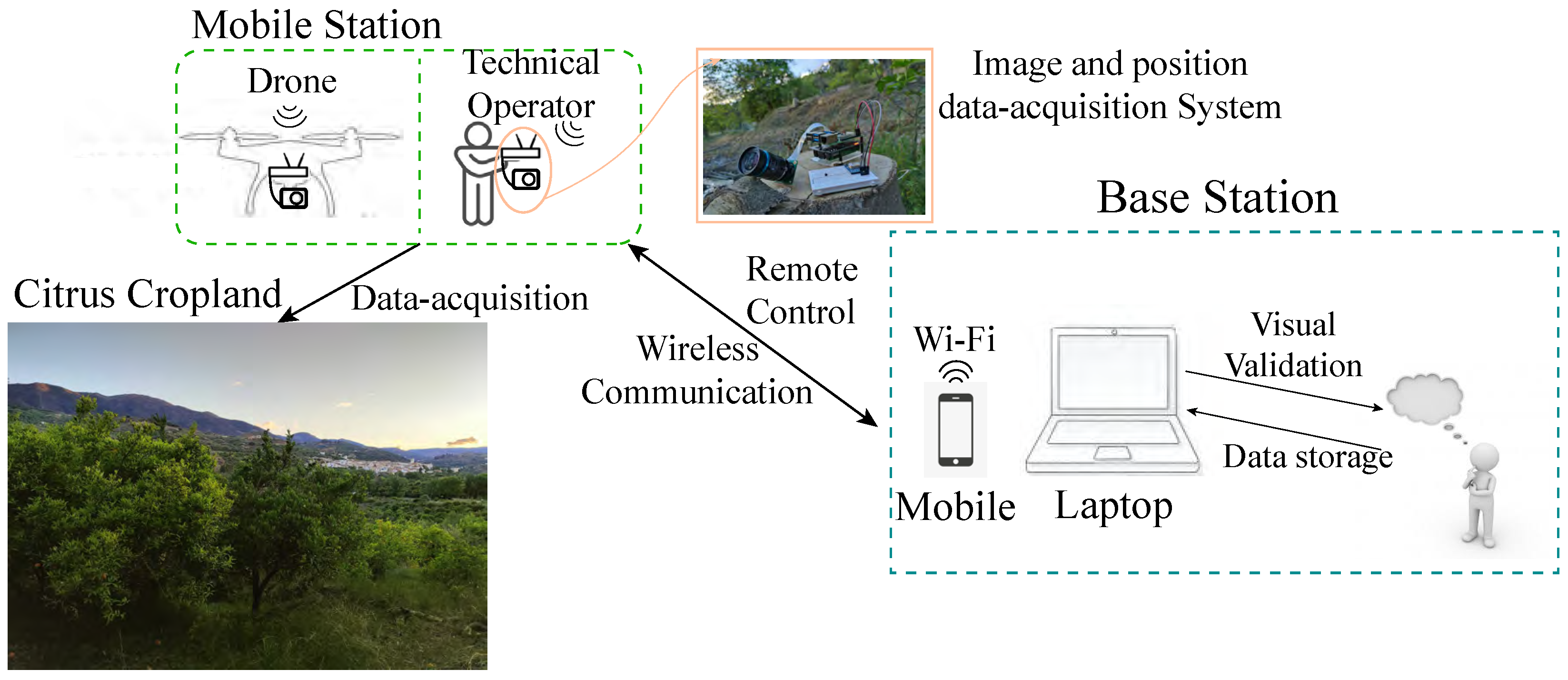
Figure 3 shows the scheme of the proposed detection system, consisting of two subsystems:

• Mobile station—Located onboard the UAV or, if necessary, operated by a technical specialist. Its main objective is to gather data for subsequent processing by the mobile station.
• Base station—Located on the ground, with the primary objective of remotely controlling the mobile station and displaying, monitoring, and processing data records.

During field tests, the following steps were taken. After setting up the hardware, the camera focus was adjusted using an HDMI-to-micro-HDMI wire connected to a screen. Then, a wireless connection between the mobile station system and the base station’s computer was established via Wi-Fi, and the VNC Viewer software was utilised for remote access to the Raspberry Pi computer for monitoring data acquisition. The field test was conducted outdoors, either with the hardware in hand or onboarded on a UAV, while geolocation positions and images were automatically saved on the inserted SD card. Finally, the data was transferred to the base station computer using WinSCP or cloud storage. The acquired data was then stored in a designated database for further analysis and processing. This systematic approach ensured effective testing and data collection for subsequent analysis.

Field tests were conducted in citrus croplands in Granada (Spain), which are mainly affected by greening and to a lesser extent woolly whitefly.

2.3. Dataset Generation

In this work, datasets were required for the following scenarios:

• Simple scenario—Simple leaves over a uniform, monochromatic background.
• Complex scenario—Leaf foliage on a natural, actual background.

A major challenge was the availability of public datasets. Not only is there a scarcity of datasets dedicated to citrus species, but the few that are available lack the necessary labelling for feeding into a network model for semantic segmentation [11,20]. This issue is particularly limiting when addressing complex scenarios, as the absence of a well-suited dataset directly impacts model performance.

To address the simple scenario, a thorough review of the most common repositories [20] and relevant surveys was conducted. Based on this research, the following datasets were selected for the simple scenario: [39,40,41,42,43]. All of them were analysed. The data used for the simple scenario in this study are available in [39,42]. They were selected since they contain images of an appropriate resolution of both healthy and diseased leaves. They were used to create a database for the simple scenario that consisted of 236 images from [39] and 566 images from [42], with resolutions of 6000 × 4000 pixels and 256 × 256 pixels, respectively. Specifically, three training datasets were created, containing 20, 60, and 90 images, respectively. The remaining images were used to create a fourth dataset for inference purposes. Given the fact that the images were not labelled, the need for manual annotation of the images cannot be denied, as stated in Section 2.4.

For the complex scenario, the DeepFruits dataset [21] stands out among more than 40 public datasets analysed because it includes images of oranges collected in open fields, among other species. This dataset was created for fruit quantification and has a small image resolution, limited volume, and lacks labelling. The myCitruss dataset [44] and Plant Diagnosis dataset [45] contain a diverse collection of citrus leaf images, including instances featuring clusters of leaves in orchard environments. These datasets have been annotated for object detection tasks. The complexity of manually annotating these ambiguous images renders them unsuitable for the purposes of this project. Instead, in this work, we built our own dataset for the complex scenario, taking high-quality photographs of citrus species in open fields under natural environmental conditions. The images were captured throughout the winter and spring at various times of the day, particularly after sunset, to ensure consistent lighting conditions. The temporal window during dataset generation enabled the capture of a wide range of phenological stages of the plant and the progression of the disease. Additionally, the images were taken under diverse conditions, including both high-resolution and slightly lower-quality leaf contours, varying image brightness, leaf tonalities, non-uniform leaf shapes and deformities, different distances from the subject, and multiple leaf orientations and inclinations. These approaches aimed to improve the model’s learning capacity, versatility, and robustness while reducing its dependence on image quality. Several resolutions were used: 4000 × 3000, 4608 × 3456, 1280 × 720, and 1024 × 768 pixels. The database consisted of 198 pictures, which were selected for deep learning training and inference purposes. Specifically, three training datasets were created, containing 30, 60, and 90 images, respectively. A fourth dataset was established for testing the proposed solution on unseen data and contained the remaining images, including those with highly complex backgrounds and those obtained from flight tests. Since these custom datasets were created from scratch, the manual annotation of images is of utmost importance, as outlined in Section 2.4.

Three different methodologies were followed to generate our database, based on performing outdoor tests in three cropland locations within the province of Granada, Spain.

The first one involved conducting field tests using the RPi data acquisition system. This not only assessed the computing module but also generated a dataset to serve as input for the recognition algorithm to verify the functionality of the proposed solution as a whole. The photographs were taken at a distance ranging from 1 m to 2 m, aiming to capture images similar to those that might be obtained from a drone. This helped verify whether the camera’s features were accurate enough to visually recognise the problem and accomplish the project’s purpose. As a result, these images were characterised by highly complex backgrounds and were used in the fourth dataset.

The second methodology was used to generate the majority of the images in the database. The outdoor tests involved different devices and distance ranges from those used in the previously mentioned tests. The hardware used to generate the database consisted of a personal mobile device with a high-resolution main camera (48 MP) and a private computer. The camera was used to capture images of the target object at different angles and distances under varying lighting and environmental conditions. The computer was then used to carefully examine each image, manually selecting and classifying it according to its quality and complexity, to facilitate the subsequent annotation task. Therefore, the final datasets reflect significant diversity, capturing various stages of the disease and different environments, including a wide range of high-quality and detailed images, as previously mentioned, making them suitable for training robust deep learning models and evaluating their performance. Regarding the distance range, the majority of photographs were captured as orthophotographs at close range to the camera lens, ranging from 25 to 35 cm, to ensure that the symptomatology and leaf contours were clearly visible, especially the anomalies and defects. In most cases, photographs were captured after sunset to ensure uniform brightness. These steps aimed to facilitate the subsequent image post-processing task and generate a robust deep learning model for the segmentation of citrus foliage. Furthermore, it was necessary to simplify the complexity of the background by avoiding high levels of foliage superposition and the presence of a large number of fruits. Hence, a simplified version of the highly complex scenario was selected to avoid ambiguities and misunderstandings and to facilitate the later image-labelling task, thus reducing the time-consuming process while ensuring an accurate and efficient solution. Additionally, photographs capturing the entire tree were taken at distances ranging from 1.5 to 2 m to evaluate the model’s performance on unseen, highly complex images.

Finally, the third methodology entailed flight tests with a small quadcopter drone. These flight tests aimed to evaluate the performance of the proposed solution on unseen images captured from a UAV and to study the challenges and limitations encountered during the operation of the mobile station. The photographs were taken at a distance ranging from 30 cm to 1 m, in order to capture images similar to those obtained using the aforementioned methodologies. This approach aimed to analyse and compare the results and draw conclusions.

Table 2. Dataset composition used to generate the best model for each scenario.

Scenario	N Images	Resolution (Pixels)	Split (N Images)			Source	Labelling Type
			Train	Validation	Test
Simple (simple leaves)	90	6000 × 4000 256 × 256	63	14	13	Open: [39,42]	Manual
Complex (field images)	90	4608 × 3456 4000 × 3000 1280 × 720 1024 × 760	63	14	13	Custom: Captured from 3 different croplands (Granada, Spain)	Manual

summarises the key characteristics and composition of the datasets for both scenarios, which ultimately supported the training and selection of the best model, as detailed in Section 3.2.

2.4. Image Annotation Task

Manually labelling a raw dataset to train the chosen segmentation network is of the utmost importance. This is a challenging task, as highlighted by [23], since although separating the plant from the background can be achieved with satisfactory accuracy, individual leaf segmentation remains a significant challenge, particularly when leaves overlap. The variety of images selected for training the neural network included both high-resolution and slightly lower-quality leaf contours, varying image brightness and leaf tonalities, non-uniform leaf shapes and deformities, and different leaf orientations and inclinations. This selection was made to improve the versatility and robustness of the model.

Several custom segmentation tools were assessed to assist with the labelling process. Non-open-source tools were rejected due to the limitations of this project. The Segment Anything Model (SAM) is a segmentation AI model system from Meta AI that can segment any object in any image with “zero-shot” performance, simply by clicking on the object without the need for additional training [28]. Despite its impressive capabilities, the SAM was rejected because it does not generate labels. “Azure Machine Learning” from Microsoft was also rejected since it only supports instance segmentation with polygon labels instead of pixel-level labelling [46].

Despite these advances, to the best of our knowledge, there are currently no widely available models capable of automatically performing pixel-level semantic segmentation annotation of the object of study. Therefore, manual labelling was necessary. The “Image Labeler App” from MathWorks was selected due to its comparable performance with other tools and its useful sub-tools for creating pixel labels.

In this work, two semantic categories, “leaf” and “background,” were considered. The methodology involved importing 2D images, defining Region of Interest (RoI) labels, manually labelling the images using tools like the “Flood Fill Tool” or the “Assisted Freehand Tool”, and correcting possible RoI errors. The RoI labels were defined by manually assigning a pixel label type and label names, such as “leaf” and “background” for the simple scenario and only “leaf” for the complex scenario, since the complexity of the images makes “background” manual labelling impractical. Thus, an original algorithm was developed to label the remaining unlabelled pixels as “background”. Finally, the labelled ground truth was then exported to a MAT file and accompanying PNG files.

Manual labelling is a laborious task that consumes significant time. After checking the performance of the current built-in automation algorithms, we found them unsuitable for accomplishing our specific needs of segmenting images from the dataset. To speed up the labelling process, a novel label-automation algorithm was developed within MATLAB 2022b as a proof of concept to explore the potential for automatic dataset labelling. MATLAB’s labelling app returns the created labels, which should subsequently be reviewed to correct minor errors. This algorithm utilises a pre-trained network to accelerate the annotation process for both “leaf” and “background” regions. Hence, the automation algorithm class was developed particularly for this case study, building upon the generic function template provided within the “Image Labeler App” to integrate pixel segmentation algorithms into the “Ground Truth Labeler” app [47,48]. The following modifications were required to customise the template. The definition of a new class extending vision.labeler.AutomationAlgorithm was essential to accommodate the specific dataset characteristics and to implement the requisite methods and functions accordingly. Notably, in the autoLabels function, the initialisation of algObj for each category was required, and the categorical range was adjusted to [0:1]. In addition, the explicit definition of classes within the semanticseg function was omitted to ensure the algorithm’s correct operation. Lastly, the intermediate step pixelCatResized was excluded to improve segmentation performance. Section 3.3 presents and discusses the performance of the label-automation algorithm. It is important to emphasise that this algorithm was introduced as a contribution aimed at streamlining the annotation process in future research. All data used for training and testing the network were manually annotated to ensure the highest possible quality and reliability of the ground-truth labels. Thus, the label-automation algorithm was not employed to generate any dataset partitions in the present study.

Several challenges were encountered during the annotation task. The highly time-consuming nature of this laborious task was the main challenge, taking around 3 min/image for the simple scenario and up to 25–40 min/image for the complex scenario when labelling only the leaf region of interest. The complexity of the scenario required manual labelling, as current pre-trained models and labelling tools were not advanced enough to handle this task effectively. Additionally, the built-in automation algorithms in MATLAB were unsuitable for automatic pixel-level annotation. Establishing an unambiguous criterion for discerning class labels at the pixel level proved to be laborious and challenging.

Despite the numerous challenges faced throughout the project, valuable insights and contributions have been made. First, the manual labelling of images entails that it is unlikely to confuse citrus leaves with other species not considered in this study. Additionally, alternative techniques such as clustering, as proposed in [26], also require manual post-processing, which is equally complex and costly, as it loses the contextual reference.

Additionally, an efficient algorithm to automatically label the background in complex scenarios has been developed, whose runtime is just 1.23 s to label a dataset of 30 images after manually annotating all pixels corresponding to the leaf class. When comparing these results with those obtained using the Segment Anything Model (SAM) API by Meta AI, this algorithm automates the process without the need for human interaction (such as clicking on the image), thereby speeding up the process and offering greater precision in capturing the object of study. Thus, the innovative label-automation algorithm developed in this work is a great contribution to the scientific community since it speeds up the labelling process of semantic segmentation in similar case studies.

2.5. Deep Learning Approach

After conducting extensive literature research, SegNet was chosen to compute semantic pixel-wise segmentation, as it exhibits superior performance, according to [49], and offers efficient memory and computational time during inference. SegNet is a Fully Convolutional Network (FCN) based on a deep encoder–decoder structure. In this work, the SegNet architecture with a VGG16 backbone is adopted to leverage pre-trained weights for improved feature extraction [50,51]. In addition, a customised PixelClassificationLayer is integrated into the network to perform per-pixel categorical predictions, enabling precise semantic segmentation tailored to the target application. This layer replaces the original pixel classification component within the network graph. Additionally, to mitigate class imbalance, it was further refined by assigning class-specific weights inversely proportional to each class’s frequency in the training set. When configured, the resulting architecture comprised 91 layers.

Although these models are not specifically trained on plant images, their general features can be fine-tuned using transfer learning to learn relevant features of citrus without overfitting. This is achieved by leveraging a pre-trained model for transfer learning. Figure 4 shows the training workflow developed to create and fine-tune the neural network. Image resizing is crucial to ensure the compatibility of dimensions between the input images and the neural network layers. Additionally, by resizing the images and pixel-label images to lower dimensions, the training time and memory usage are reduced. This aspect is of utmost importance when the computer capacity is a limitation. For this purpose, the MATLAB’s imresize function is used.

The network architecture can be designed differently based on the approach selected. Both the simple and complex scenarios primarily use the segnetLayers function. An alternative approach for the complex scenario involves using the layerGraph functions and fine-tuning the pre-trained network that exhibited the most efficient performance in the simple scenario. However, this option was not considered viable in this work due to computational limitations on available RAM. In addition, to determine the optimal hyperparameter configuration, an extensive set of training experiments was carried out. The Stochastic Gradient Descent with Momentum “sgdm” optimiser was chosen for the training process due to its favourable convergence behaviour and results reported in similar segmentation tasks [26]. For more details on the architecture settings and training configurations for each model variant, please consult

Table A1. Model parameters for the simple scenario.

Simple Scenario
Model	1	2	3	4	5	6	7	8	9	10
No. of Images	20	20	60	60	60	60	90	90	90	90
Resize [height, width]	[320, 480]	[320, 480]	[320, 480]	[320, 480]	[256, 256]	[256, 256]	[320, 480]	[320, 480]	[320, 480]	[320, 480]
Data Splitting (%)	70-15-15	70-15-15	70-15-15	70-15-15	70-15-15	70-15-15	70-15-15	70-15-15	70-15-15	70-15-15
Data Aug. [+/− Pixels]	-	-	-	-	-	-	-	10	10	20
Class Weighting	-	-	-	-	-	-	-	Yes	Yes	Yes
Optimiser	sgdm	sgdm	sgdm	sgdm	sgdm	sgdm	sgdm	sgdm	sgdm	sgdm
MiniBatchSize	4	4	4	4	4	4	3	3	3	3
Max. No. Epochs	30	30	30	55	30	55	30	30	55	55
Learning Rate	0.01	0.01	0.01	0.01	0.01	0.01	0.01	0.01	0.01	0.01
L2 value	${10}^{-4}$	${10}^{-4}$	${10}^{-4}$	${10}^{-4}$	${10}^{-4}$	${10}^{-4}$	${10}^{-4}$	${10}^{-4}$	${10}^{-4}$	${10}^{-4}$
Validation Freq.	20	20	20	20	20	20	20	20	20	20

–

Table A3. Model parameters for complex scenario 2.

Complex Scenario (2/2)
Model	10	11	12	13	14	15	16	17	18
Dataset Name	Subsets 1 and 2	Subsets 1 and 2	Subsets 1 and 2	Subsets 1 and 2	Merged	Merged	Merged	Merged	Merged
No. of Images	60	60	60	60	90	90	90	90	90
Resize [height, width]	[375, 500]	[375, 500]	[375, 500]	[375, 500]	[375, 500]	[375, 500]	[375, 500]	[375, 500]	[375, 500]
Data Splitting (%)	60-20-20	70-15-15	60-20-20	70-15-15	70-15-15	70-15-15	70-15-15	70-15-15	70-15-15
Data Aug. [+/− Pixels]	-	-	10	10	10	25	30	10	30
Class Weighting	Yes	Yes	Yes	Yes	Yes	Yes	Yes	Yes	Yes
Optimiser	sgdm	sgdm	sgdm	sgdm	sgdm	sgdm	sgdm	sgdm	sgdm
MiniBatchSize	3	3	3	3	3	3	3	3	3
Max. No. Epochs	30	30	30	30	30	35	30	30	30
Learning Rate	0.01	0.01	0.01	0.01	0.01	0.01	0.01	0.1	0.01
L2 value	${10}^{-4}$	${10}^{-4}$	${10}^{-4}$	${10}^{-4}$	${10}^{-4}$	${10}^{-4}$	${10}^{-4}$	${10}^{-4}$	${10}^{-3}$
Validation Freq.	20	20	20	20	20	20	20	20	20
Val. Patience	3	3	3	3	3	3	3	3	3

in the Appendix A.

2.6. Workflow of the Complete Main Program

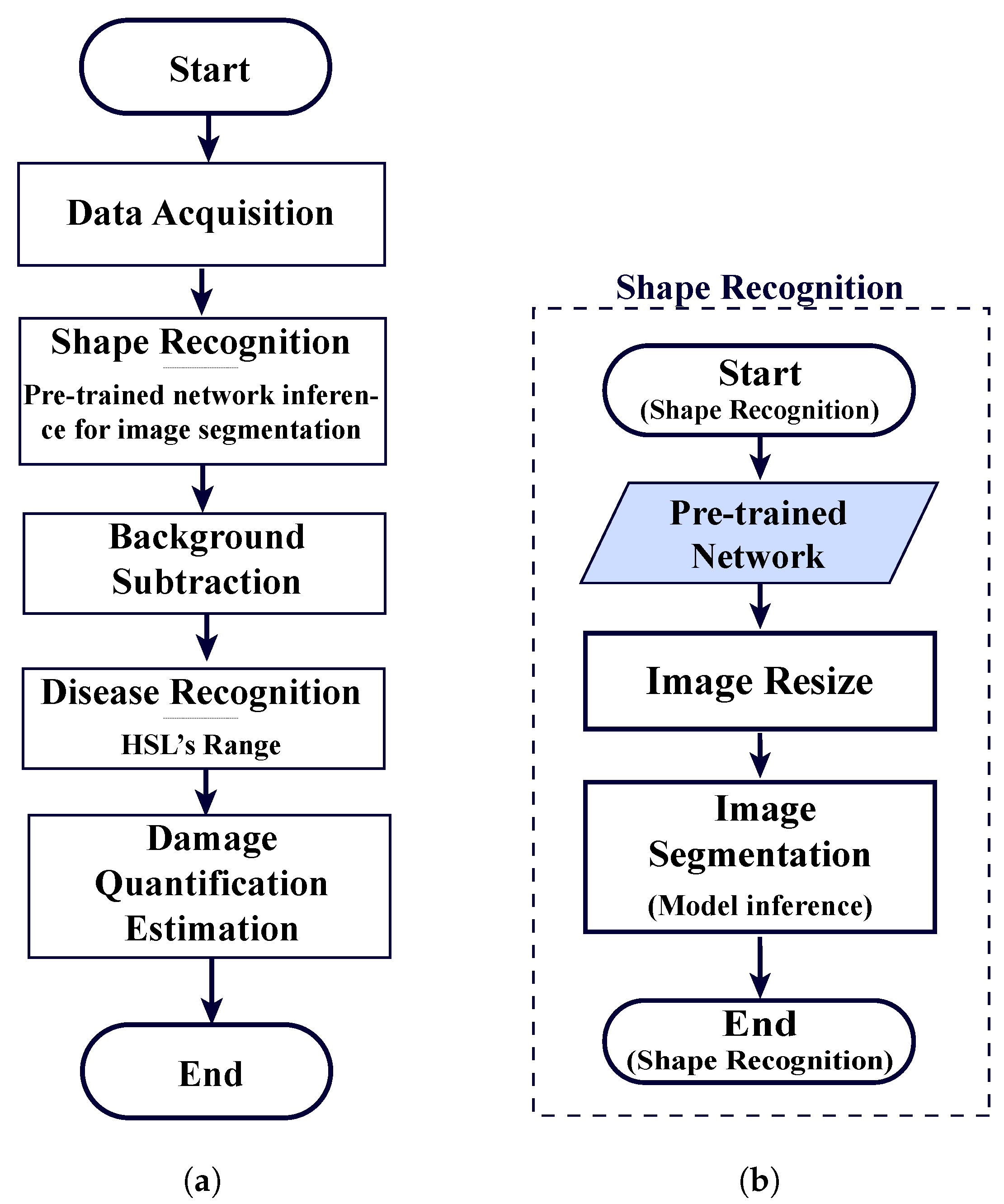
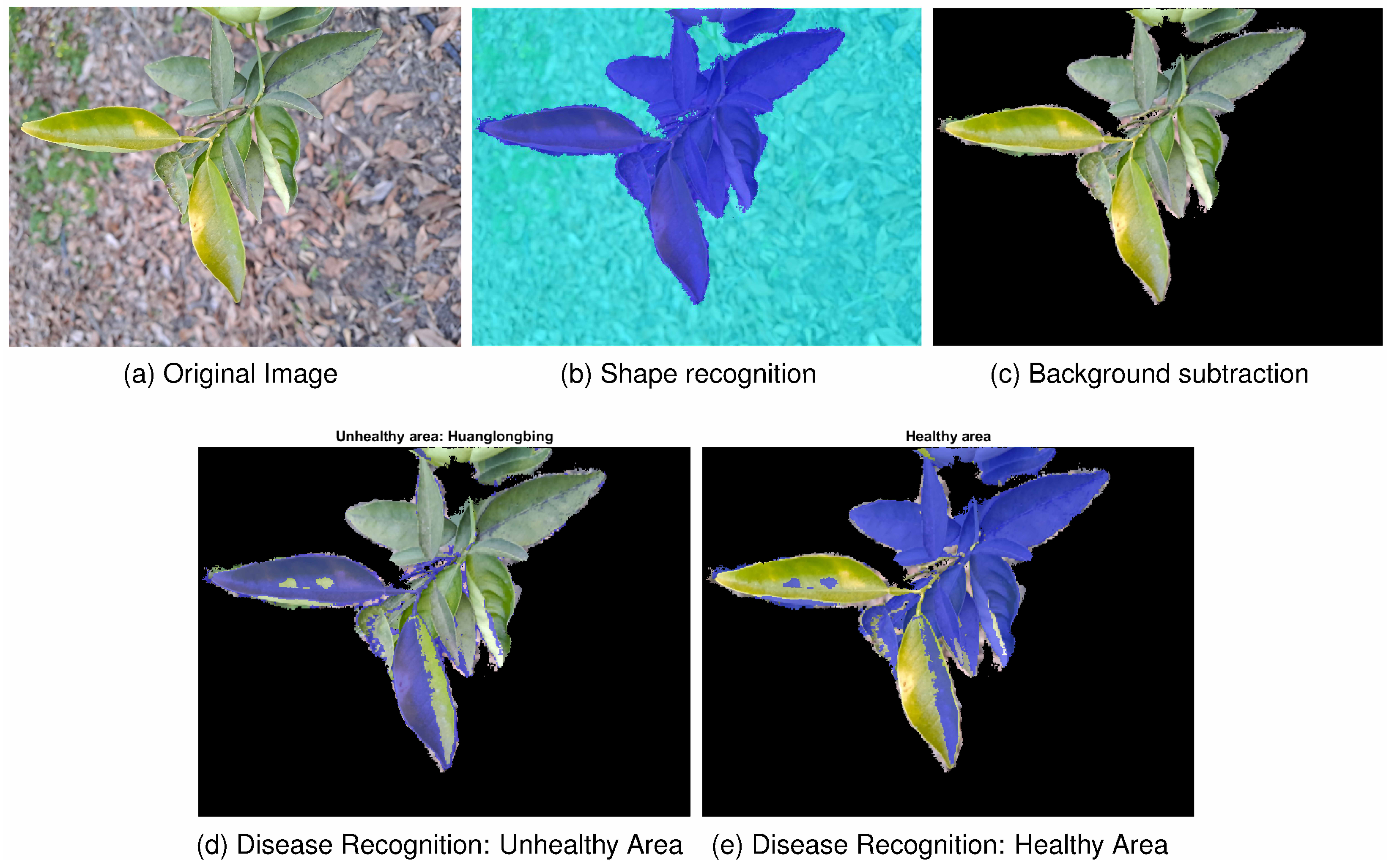
The goal is to replace the shape recognition algorithm presented in our previous research [18] with a new neural network that can accurately segment unseen data. Thus, the aim is to create a model that can generalise well beyond the training data and provide reliable and meaningful predictions in real-world scenarios. Figure 5 illustrates the comprehensive workflow encompassing the model’s inference and the integration with the rest of the modules in the complete program.

The data acquisition module automates the loading process of raw images from a dataset. While this module shares similarities with the “image reading” module presented in our previous research [18], it offers a more efficient and automated approach. Unlike manual loading, it can process unseen data without the need for manual parameter settings, eliminating the requirement to process one image at a time. This is advantageous, since manually tuning parameters for each image is a time-consuming and unpredictable task.

The shape recognition module comprises the semanticseg function, which utilises custom pre-trained networks that were previously fine-tuned for the simple and complex scenarios (refer to Section 2.5). This enables the module to make inferences with newly unseen data. Additionally, these input images are resized to match the size of the network layers. Figure 5b illustrates the workflow of the shape recognition module, highlighting its simplification concerning the approach proposed in our previous research [18]. The concept, general structure, and flowchart of the remaining modules within the main program remain unchanged from those presented in [18]. Additionally, in order to adapt the shape recognition module to the workflow, background subtraction was required. 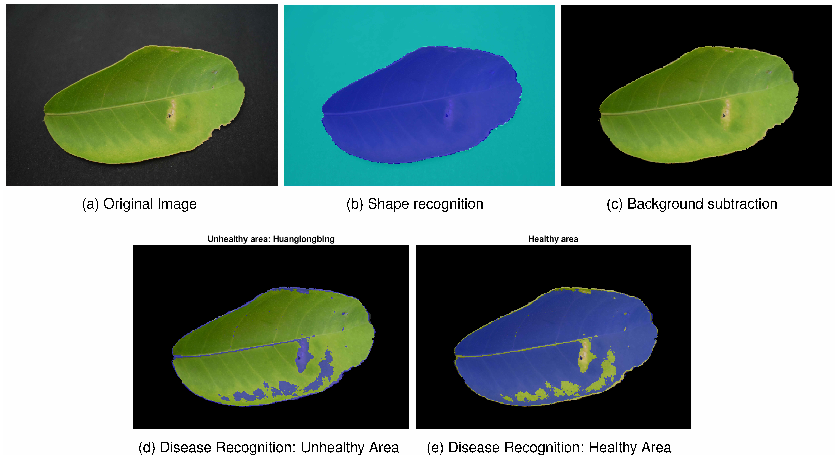While this module is equivalent to the “object RGB reconstruction” module from our previous research [18], it differs in using the label mask obtained from the previous step to isolate the object of interest from the original image. This aspect is crucial, as the disease recognition module relies on colour-based thresholding for classification. Specifically, the RGB pixel values in the image are extracted and classified as either “unhealthy” or “healthy” areas based on predefined ranges of the HSL colour space for Huanglongbing disease [18]. The HSL’s model binds the attributes and morphology of leaves together. In other words, the colour associated with the diseased part of the leaf and the green colour associated with its healthy part can be narrowed down to an approximate range of tones in the regions of interest. The HSL’ model range determined for this case study is presented in

Table 3. HSL’s model range.

Region of Interest	Healthy Leaf	Huanglongbing Symptoms
Characteristics	Green colour	Leaf discolouration and yellow blotches
Hue Range (H)	H ⊆ [73: 222]	H1 ⊆ [35: 45] ∪ H2 ⊆ [46: 72]
Saturation Range (S)	Unconstrained	Unconstrained
Lightness Range (L)	Unconstrained	L1 ⩾ 40 ∪ L2 ⩾ 25

. Lastly, the damage quantification module estimates the damage threshold, quantifying the proportion of healthy and unhealthy leaf areas based on the pixel-level classification results. Our previous research [18] demonstrated the effectiveness of the proposed methodology.

Hence, to summarise, the complete algorithm can detect the damage present in the leaves at a pixel level by utilising the trained model to segment the leaf contour.

This methodology can be applied to other citrus phytosanitary problems, such as woolly whitefly or citrus canker [52,53], by determining their corresponding HSL model ranges that particularise their symptoms. Furthermore, the applicability of this methodology can be extended to other species by fine-tuning the network with custom datasets.

However, the scarcity of databases specifically dedicated to capturing plant species in a natural environment, particularly citrus, as outlined in Section 2.3, poses a significant challenge. This issue is further compounded by the lack of publicly available, labelled datasets suitable for training network models to perform semantic segmentation. These limitations underscore the remarkable contributions of this study.

In addition, as discussed in Section 1.3, the effectiveness of segmentation approaches varies widely depending on the specific species and environmental conditions, suggesting that findings may not generalise across studies. Leaf detection and segmentation is a complex image segmentation problem [54]. Consequently, meaningful comparisons with similar research are inherently challenging.

3. Results

3.1. Data Acquisition System Results

To assess the image quality of the Pi’s camera modules, the performance of the GPS module, the signal range, and the PiPower’s battery capacity, various experiments were conducted, both indoors and outdoors.

During the indoor test, both cameras were tested under the same conditions: the data acquisition system was placed at a distance of approximately 30 cm on a table to prevent motion. A screen was used to manually adjust the image focus. After analysing the results, it can be concluded that the quality of the data acquired from the cameras was sufficient for accomplishing the objectives of this project, and the high-quality camera captured the images with higher definition and clarity than Camera Module V2, as expected.

During the outdoor tests, it was not possible to test both cameras under the same environmental and physical conditions. Images were captured at distances ranging from 1 to 2 m from the nearest leaves while holding the complete system manually on the ground or at a fairly high position simulating drone flight. However, these field tests presented several challenges, including the need for a wired connection between the RPi board and a screen to preview the camera image and the difficulty of adjusting the camera focus while holding the entire system. After thoroughly analysing the photographs, the same conclusions can be drawn, highlighting that the image quality was sufficient for visually recognising the symptomatology of the object of study. Hence, it can be concluded that the camera was able to capture clear and detailed images up to a distance of 2 m when exposed to different luminosity conditions. The image quality was sufficient for recognising the symptomatology, even in the worst case studied. Therefore, the drone should take photographs at a distance of around 1 m or 1.5 m from the tree top to distinguish the symptoms of the disease.

During the outdoor field test, determining a precise position in terms of latitude and longitude was a fast task, requiring just over 3 s. The atomic clocks of the GPS satellites provide highly precise time data to the GPS signals and synchronise each receiver. However, since the altitude determined by the Global Navigation Satellite System (GNSS) is not accurate enough and may imply a risk to controlling and measuring the distance between the crop top and drone during the flight, the study and implementation of a backup system that provides more precision in terms of altitude are proposed as a future line of research. To conclude, the wireless communication range for outdoor settings is a radius of approximately 95 m. Nonetheless, when the system is partially or completely covered indoors, the range decreases to a radius of 65 m, and even lower when more obstacles are present.

3.2. Segmentation Results

To evaluate the performance of the segmentation model under different conditions, two distinct test scenarios were considered. The first one, referred to as the simple scenario, involved a small set of citrus leaves placed against a uniform background under controlled lighting conditions. This setup was used as a proof-of-concept experiment to validate the functionality of the system and to assess the base performance of the network architecture with minimal visual complexity. The second and more relevant scenario, referred to as the complex scenario, involved images acquired from real citrus crops under natural lighting and heterogeneous background conditions.

3.2.1. Simple Test Scenario (Controlled Conditions)

For the simple scenario, three datasets, each consisting of 20, 60, and 90 images, were used to train the models. The two initial datasets were based on a publicly available database [39] (referred to as “Database 1”), while the dataset of 90 images combined “Database 1” with a second publicly available database [42] (referred to as “Database 2”). These datasets were used to train nine different deep learning models, whose results are displayed in

Table 4. Deep learning accuracy results for the simple scenario.

Simple Scenario
Model	1	2	3	4	5	6	7	8	9	10
Validation Accuracy (%)	98.69	98.79	99.37	99.46	98.97	98.90	98.90	99.41	99.46	99.39
Training Accuracy (%)	99.16	99.28	99.56	99.77	99.53	99.74	99.50	99.24	99.47	99.43
Global Accuracy (%)	98.62	98.71	99.32	99.42	99.02	99.02	98.92	99.47	99.54	99.41
Recall (%)	98.08	98.15	98.23	98.40	97.39	97.14	97.04	99.28	99.37	99.30
IoU (%)	94.49	94.79	97.10	97.49	95.83	95.78	95.99	98.05	98.28	98.16
F1-Score (%)	85.11	86.51	93.92	94.68	87.31	87.13	89.79	98.24	98.78	98.65
Leaf Class Recall (%)	97.33	97.39	96.74	97.01	95.16	94.60	94.28	99.00	99.12	99.15
Background Recall (%)	98.83	98.91	99.72	99.78	99.61	99.69	99.79	99.56	99.61	99.45
Validation Loss	0.135	0.133	0.049	0.032	0.058	0.044	0.051	0.037	0.034	0.042

. For details on the architecture parameters and training options used for each model, please see Table A1 in the Appendix A. To aid reader comprehension, the parameter “Data Split” indicates the percentage distribution of the data across the training, validation, and test datasets. Likewise, “Image Dataset Size” refers to the dataset volumes outlined in Section 2.3.

After training, a balance of the metrics presented in Table 4 was used to select the best-suited model, with particular emphasis on low validation loss and high validation accuracy. For each class, recall is defined as the ratio of correctly classified pixels, based on the ground truth, to the total number of pixels in that class. Global accuracy refers to the proportion of all pixels that are correctly classified relative to the total, regardless of their class. Additionally, the F1-score, Intersection over Union (IoU), and recall were computed as the average across all classes. These metrics were computed using the test dataset.

The best model for the simple scenario, Model 9 (refer to Table 4), achieved the highest validation accuracy (99.46%) and the lowest validation loss. All evaluation metrics fell below the 0.05 threshold, indicating strong performance. Likewise, the test accuracy closely matched the training and validation accuracy, indicating that the model performed well not only on the training data but also on unseen test data. These conclusions are further supported by the metrics of Model 9, as detailed in Table 4. Moreover, it is worth noting that, although other models exhibited overall high performance and similar validation accuracies, there were indicators of overfitting. Specifically, the “TrainingProgressMonitor” of MATLAB displayed that the training accuracy slightly exceeded the validation accuracy and that the training loss was lower than the validation loss. Lastly, overfitting was observed during the inference of the model, as it became too specialised in the training data and performed poorly on unseen data. To address these limitations, the dataset of 60 images was augmented with 30 additional images from Database 2, and “class weighting” and “data augmentation” techniques—including rotation, flipping, translation, reflection, and brightness adjustments—were implemented (refer to Table A1). The following conclusions were drawn: Resizing the images slightly affected the model’s performance and the elapsed time; hence, it is preferable to train the model using higher-resolution input images if the system can handle it. Increasing the maximum number of epochs did not necessarily result in a significant improvement, and the GPU substantially accelerated the training process.

As outlined in Section 2.6, the specificity of this case study and the scarcity of suitable datasets focused on citrus leaf segmentation, combined with the inherent complexity of leaf detection and segmentation, present a substantial challenge in drawing direct comparisons with similar studies. Nonetheless, to establish a benchmark, the performance of this approach was compared with existing segmentation techniques that were trained on non-citrus species. The leaf segmentation recall achieved by our method was 99.12%, surpassing the single-leaf segmentation rate of 95.34% reported in [54], indicating a notable improvement. Furthermore, the proposed method significantly outperformed the highest accuracy of the common segmentation-based techniques reported in [55], such as the “simple and triangle thresholding” method, which reached 98.6%.

3.2.2. Complex Scenario

For the complex scenario, due to system limitations, a new model based on a SegNet architecture with a VGG16 backbone was trained. Our three datasets were used (refer to Section 2.3), each consisting of 30 manually and specifically selected images, distinct from the others, carefully chosen to address the complexities of the scenario. Furthermore, the datasets were merged to generate larger volumes of data, resulting in two more datasets comprising 60 and 90 images. Likewise, these datasets were used to train eighteen different deep learning models, whose results are displayed in

Table 5. Deep learning accuracy results for the complex scenario (1/2).

Complex Scenario (1/2)
Model	1	2	3	4	5	6	7	8	9
Validation Accuracy (%)	83.09	84.40	88.71	91.17	90.71	91.40	89.32	91.86	92.83
Training Accuracy (%)	93.89	94.65	95.61	97.73	97.10	98.22	96.61	97.87	97.62
Global Accuracy (%)	81.55	81.26	82.04	91.44	92.80	91.02	89.15	90.13	89.95
Recall (%)	75.27	76.97	78.65	88.50	90.88	88.97	86.93	88.05	86.82
IoU (%)	63.82	64.74	66.36	81.73	84.67	81.17	79.33	82.19	78.98
F1-Score (%)	49.93	54.37	57.61	65.07	67.59	67.51	65.42	65.68	62.97
Leaf Class Recall (%)	56.98	64.02	68.40	80.39	85.47	83.45	83.27	82.40	78.05
Background Recall (%)	93.55	89.92	88.89	96.62	96.29	94.45	90.59	93.69	95.58
Validation Loss	0.385	0.366	0.283	0.232	0.241	0.221	0.270	0.212	0.191

and

Table 6. Deep learning accuracy results for the complex scenario (2/2).

Complex Scenario (2/2)
Model	10	11	12	13	14	15	16	17	18
Validation Accuracy (%)	92.28	91.83	93.87	93.35	94.59	95.06	94.82	95.56	94.03
Training Accuracy (%)	97.23	94.24	95.85	94.59	95.67	95.49	95.33	96.88	92.02
Global Accuracy (%)	88.99	90.33	91.36	92.04	93.01	93.98	93.60	93.30	92.41
Recall (%)	88.54	90.31	91.36	92.22	93.03	93.78	93.57	92.50	93.04
IoU (%)	78.25	80.56	82.52	83.66	85.64	87.42	86.74	85.99	84.67
F1-Score (%)	59.85	64.11	67.05	71.04	74.67	79.03	77.08	77.09	72.28
Leaf Class Recall (%)	87.29	90.26	91.35	92.71	93.09	93.20	93.47	90.21	94.87
Background Recall (%)	89.79	90.37	91.37	91.73	92.97	94.36	93.67	94.80	91.22
Validation Loss	0.221	0.254	0.179	0.199	0.159	0.142	0.153	0.143	0.160

. A detailed explanation of the evaluation metrics employed can be found in Section 3.2.1. For details on the hyperparameters, dataset configurations, and training options considered for each model, please see

Table A2. Model parameters for complex scenario 1.

Complex Scenario (1/2)
Model	1	2	3	4	5	6	7	8	9
Dataset Name	Subset 1	Subset 1	Subset 1	Subset 2	Subset 3	Subsets 1 and 2	Subsets 1 and 2	Subsets 1 and 2	Subsets 1 and 2
No. of Images	30	30	30	30	30	60	60	60	60
Resize [height, width]	[320, 480]	[375, 500]	[375, 500]	[375, 500]	[375, 500]	[375, 500]	[375, 500]	[375, 500]	[375, 500]
Data Splitting (%)	70-15-15	70-15-15	70-15-15	70-15-15	70-15-15	70-15-15	70-15-15	80-10-10	60-20-20
Data Aug. [+/− Pixels]	-	-	-	-	-	-	-	-	-
Class Weighting	-	-	-	-	-	-	-	-	-
Optimiser	sgdm	sgdm	sgdm	sgdm	sgdm	sgdm	sgdm	sgdm	sgdm
MiniBatchSize	4	2	3	3	3	3	3	3	3
Max. No. Epochs	30	30	30	30	30	30	30	30	40
Learning Rate	0.01	0.01	0.01	0.01	0.01	0.01	0.005	0.01	0.01
L2 value	${10}^{-4}$	${10}^{-4}$	${10}^{-4}$	${10}^{-4}$	${10}^{-4}$	${10}^{-4}$	${10}^{-4}$	${10}^{-4}$	${10}^{-4}$
Validation Freq.	20	20	20	20	20	20	20	20	20
Val. Patience	2	2	2	2	2	2	2	5	3

and Table A3 in the Appendix A.

The best model for the complex scenario, Model 15 (detailed in Table 6), was selected based on a balanced combination of metrics, rather than relying on a single metric. It is worth noting that the accuracy was lower than the 5% error threshold, and the validation loss slightly exceeded 10%. Specifically, Model 15 achieved the lowest validation loss of all experiments, along with a validation accuracy of 95.06% and a leaf segmentation recall of 93.20%. This indicates superior performance in accurately detecting and segmenting leaves compared to models with a similar metric distribution, such as Model 17. Indeed, the high test global accuracy (93.98%) and recall (93.78%), which were below the 10% error threshold, indicate that the model performed quite well on unseen test data. In addition, the model achieved a high degree of overlap between predicted and ground-truth regions, as evidenced by an IoU of 87.42%, while maintaining a balanced performance between precision and recall, with an F1-score of 79.03%. This suggests that the proposed approach is both accurate and robust, though further improvements may enhance its overall performance.

Despite the notable constraints in terms of the system limitations associated with GPU memory capacity and the available data’s quality and quantity for this specific study, this simple and potentially promising solution demonstrates that even with a modest amount of data, it is possible to achieve an appropriate and reliable model that yields efficient results. Fine-tuning the current model with a higher volume of data that considers different situations will be crucial for improving the network’s reliability and increasing its robustness. However, due to time limitations, this enhancement is proposed as a future line of research.

Based on the positive impact observed when increasing the image resize scale for the simple scenario, and given the system’s capacity, the maximum scale that we could consider was one-eighth of the majority image size in our database, which was 4000 × 3000 pixels (see Models 1 and 2 in Table A2). It is also important to maximise the MiniBatchSize within the system to improve accuracy. A balance between incorporating new data and maintaining comparable results was observed. However, the training accuracy slightly exceeded the validation accuracy and exhibited significant discrepancies compared to the test metrics, as displayed in Table 5, which indicates the possibility of overfitting. Thus, merging the datasets was considered as a solution to increase the volume of data. In addition, the inclusion of class weighting significantly improved the accuracy of the leaf class, and the data augmentation function, as described in Section 3.2.1, led to an overall improvement in accuracy, particularly for the 70% data split.

Comparing our approach with similar studies is particularly challenging for the complex scenario due to the inherent difficulties in leaf detection. Leaves are often found in groups against a natural background, where the surrounding vegetation shares similar colours and textures with the object of study. To establish a benchmark, we compared the performance of our method with a similar study focused on citrus species [26]. Our approach outperformed the results obtained using the two techniques employed in that study. The test accuracy achieved with the SVM method was 83.09%, and with deep learning techniques, it was 85.05%, whereas our solution achieved a higher test global accuracy of 93.98%, demonstrating a notable improvement. Additionally, the leaf segmentation recall of 93.20% achieved by our method surpassed the overall leaf segmentation rate of 90.46% reported in [54], which employed a model trained on non-citrus species. These results emphasise the contributions and effectiveness of the proposed methodology.

Hence, to summarise, the models selected for this work were Model 9 for the simple scenario and Model 15 for the complex scenario.

3.3. Label-Automation Algorithm Results

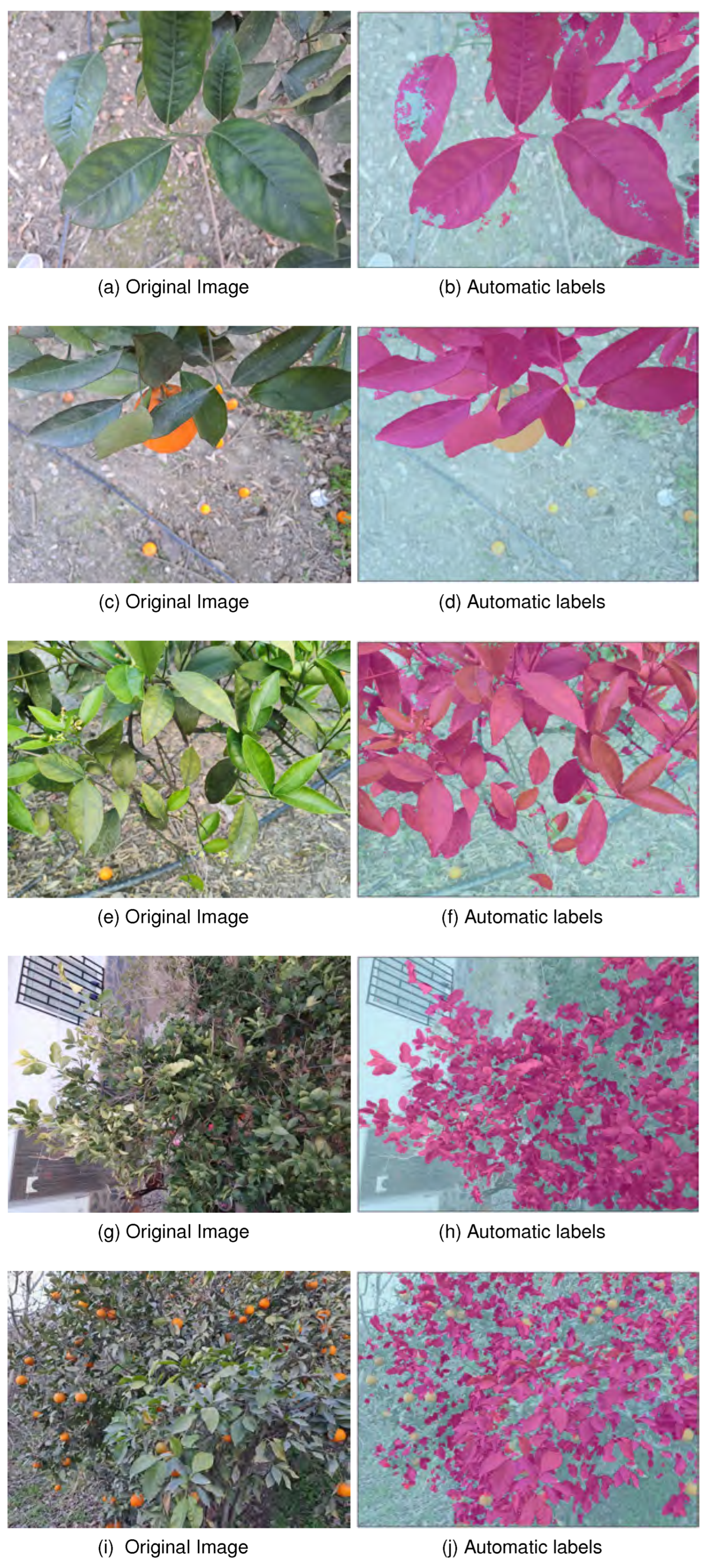
The most suitable pre-trained network was implemented within the developed label-automation algorithm. Then, the automation session was run in the MATLAB labelling app and evaluated on unseen data with different features, producing the results displayed in Figure 6.

It is crucial to note the necessity of resizing images before attempting automatic annotation to avoid errors associated with GPU memory limitations. In this regard, an NVIDIA GeFORCE GTX 1660 SUPER with 6 GB of GPU memory, 32 GB of RAM, and an AMD Ryzen 5 3600 6-core processor with 3.95 GHz of maximum frequency was used. After conducting several tests to study the limitations, it was determined that a scale of $1/2$ for an image size of 4000 × 3000 pixels could be applied within the used system’s capacity.

In Figure 6, the “pink” mask represents the pixels recognised as the leaf class, whereas the “blue” mask represents the background class. It is worth noting that all the images used for testing were unseen by the pre-trained network, and some of them even presented scenarios that were very different from those considered in the training data. These images were carefully selected to cover a range of complexities, starting from the simplest or clearest scenario and gradually increasing in complexity to include more detailed features such as tree foliage. This sequence allowed for a comprehensive analysis of the model’s performance across different levels of complexity.

In cases where there was no excessive brightness and even dense vegetation, the automation algorithm yielded promising results. Small corrections were manageable and could be easily refined during the post-processing stage. However, it can be observed that the algorithm introduced slight noise into the image. Additionally, the network encountered difficulties in recognising leaves under high-brightness or luminosity conditions. However, the observed limitations can be addressed by fine-tuning the model with a larger volume of data or during the post-processing phase. Figure 6g,i show images captured using the proposed image data acquisition system, demonstrating its practicality and efficiency in terms of compatibility with the software developed for data processing at the base station.

3.4. Inference and Results of the Main Program

This section presents some of the results obtained, both numerical and graphical, from testing the main program on unseen datasets.

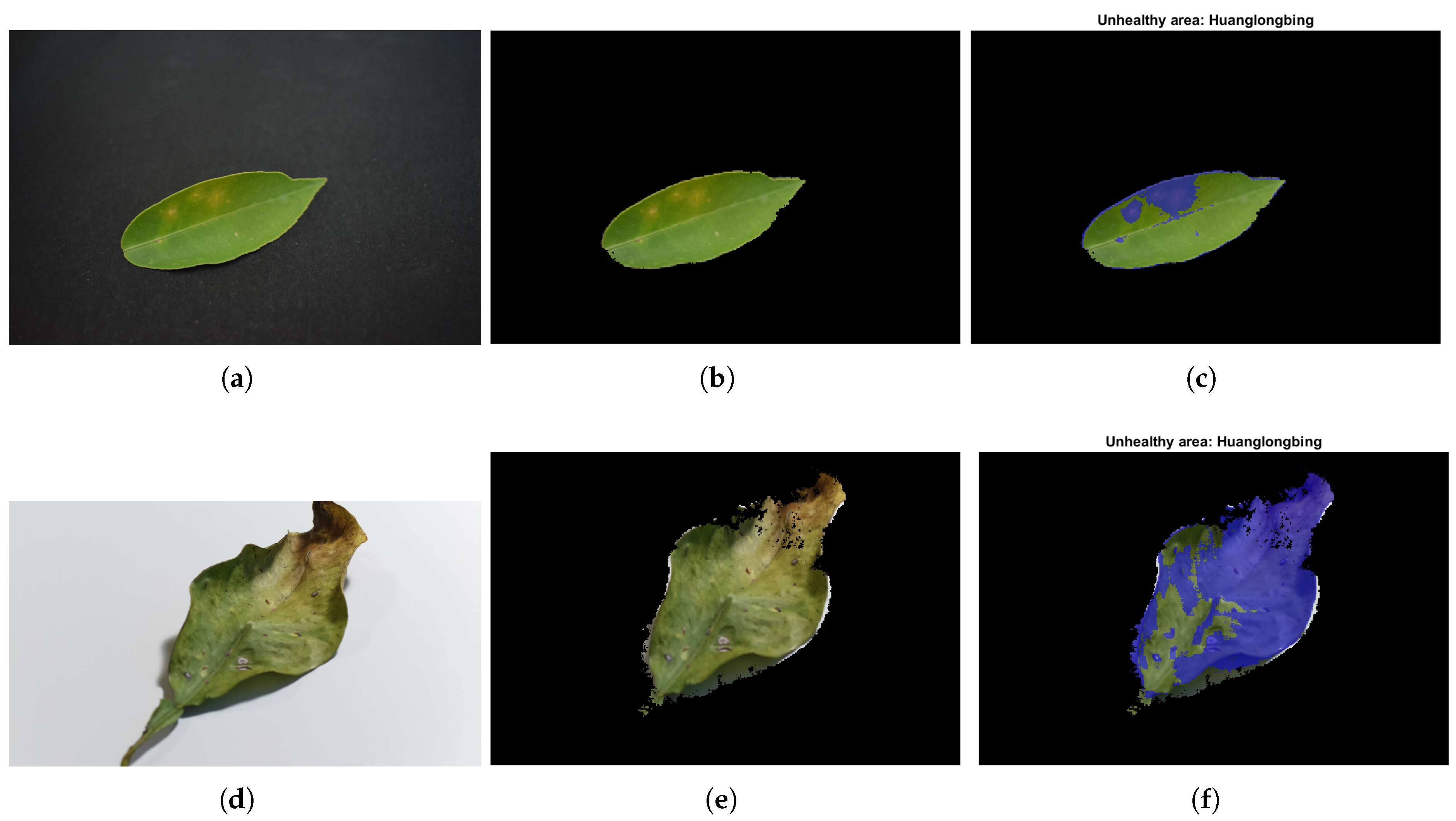
For the simple scenario, Figure 7 demonstrates the promising precision of the model in predicting unseen data and the accurate performance of the complete system in recognising the studied disease. The percentages of healthy and unhealthy areas were $P_h=87.17\%$ and $P_{uh}=12.83\%$. The unrecognised area accounted for only $P_{nr}=0.0075\%$. The execution of the complete main program workflow for this image—including data processing and image analysis—was executed on the workstation and took approximately 6 s, with the shape recognitionmodule being the most time-consuming. The execution time of the current algorithm represents a significant improvement compared to our previous research [18], in which it took approximately 80 s for the simple scenario. Additionally, it is important to note that this algorithm was designed to handle a complete dataset. The end-to-end runtime for processing a dataset of 12 images was slightly over 10 s. These analyses were conducted using 30 images from the fourth dataset, demonstrating consistent and equivalent performance. Specifically, it is worth mentioning that the percentage of pixels not recognised in either case did not exceed a 5% error rate, indicating a satisfactory accuracy level in the recognition process. For additional results demonstrating the performance of the main program on unseen data, please refer to Figure A1 in the Appendix B.

Regarding HSL’s model range, it might be beneficial to reanalyse and redefine the ranges to further refine the consideration of the unhealthy area.

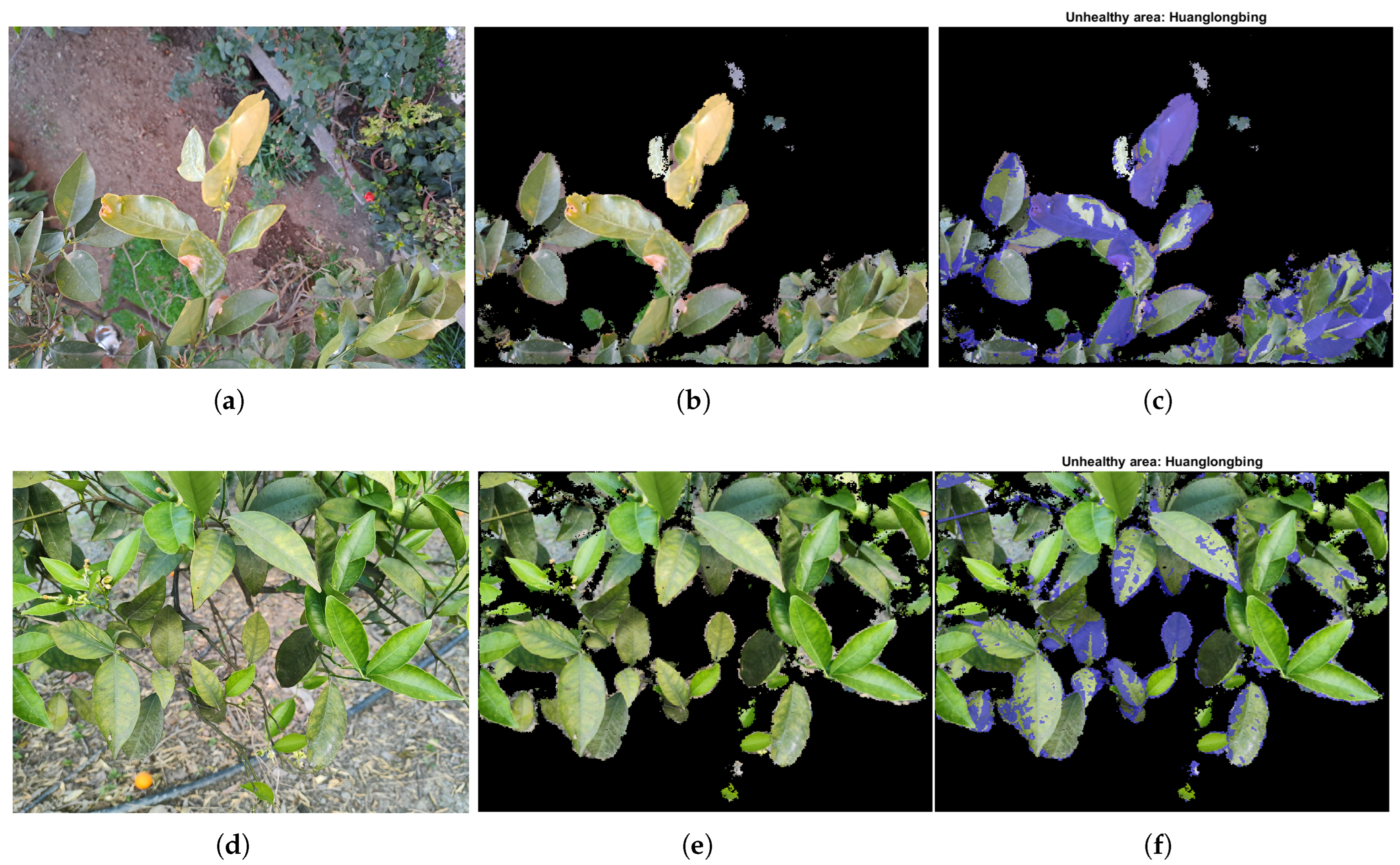
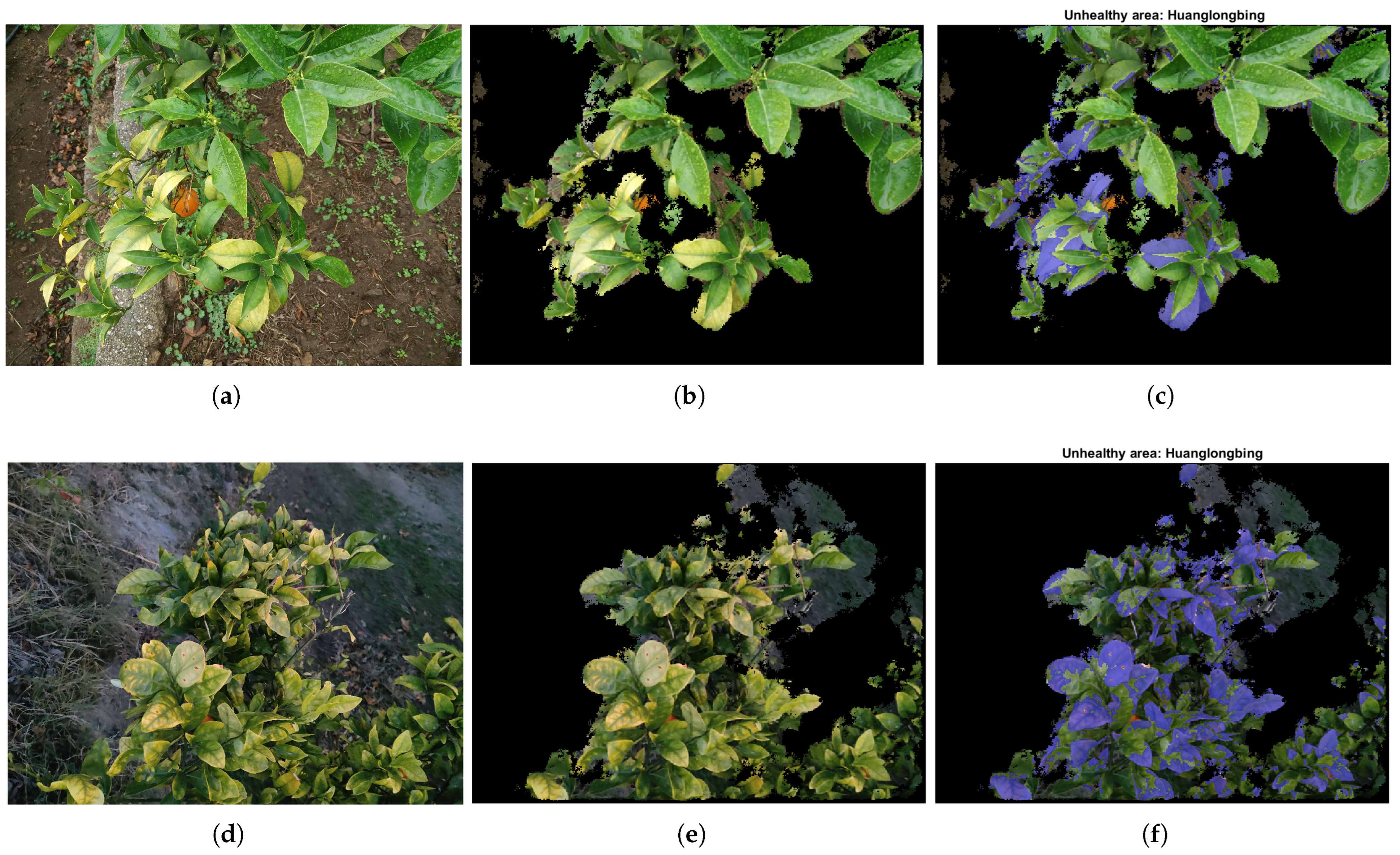
For the complex scenario, Figure 8 shows the satisfactory precision achieved by the selected best model in meeting the project objectives, particularly in accurately predicting unseen data, even with limited training images. The percentages of healthy and unhealthy areas were $P_h=69.06\%$ and $P_{uh}=30.94\%$, while the percentage of unrecognised pixels was $P_{nr}=5.63\%$. The time required to execute the main program from end to end on the workstation was similar to that of the previously analysed case, taking approximately 7 s for this image. The noteworthy reduction in the runtime of the current program, compared to our previous research [18], where processing a complex scenario image took approximately 120 s, represents a significant contribution. Additionally, computing a complete dataset of 14 images resulted in a runtime of over 16 s, significantly reducing the time required to process the same data. These analyses were conducted using 48 images from the fourth dataset, demonstrating that the overall performance of the complete system aligns with the conclusions drawn earlier, further highlighting its efficiency and effectiveness. Specifically, it is worth mentioning that the percentage of unrecognised pixels generally did not exceed a 5% error rate and, in both cases, did not exceed a 10% error rate, indicating a satisfactory accuracy level in the recognition process. For additional results demonstrating the performance of the main program on highly complex unseen data, please refer to Figure A2 in the Appendix B.

In general, the segmentation methods performed accurately with elements such as trunks, branches, fruits, grass and floor vegetation. False negatives with leaves in regions of problematic illumination have also been reported, and false positives were found with fruits and green branches. However, due to the limitation that represents the size of the dataset, the model may not fully exploit its potential to recognise the wide range of shapes and textures of the elements of interest. Hence, a larger training set is expected to improve the accuracy of the deep learning model. Specifically, including cases in the training dataset where the model has shown poorer results is considered important. This approach is proposed as a future line of research to encourage the model to extract distinguishing features that can enhance discrimination and optimise the monitoring parameter.

3.5. Remarks on UAV Flight Tests

This section presents the results of the main program after evaluating it on unseen data captured from a UAV and the influence of flight test challenges on the performance of the proposed solution. Specifically, these analyses were conducted using 25 images captured from the drone under diverse environmental conditions.

Our findings indicate that the stability of the UAV is a crucial factor for capturing clear, high-resolution images. These high-quality images significantly enhance the system’s capability for precise leaf segmentation and accurate disease detection. Furthermore, our robust model has been trained on images that exhibit unfavourable conditions, such as slightly lower-quality leaf contours and non-uniform leaf shapes and deformities. As a result, the model demonstrated proficiency in recognising and resolving images with slightly lower-quality leaf contours. Moreover, it effectively handled images with greater complexity than those used for training. Figure 9 illustrates these results and demonstrates the promising precision of the model in predicting unseen data captured from the UAV. These results further showcase the system’s adaptability and reliability in real-world scenarios.

Some limitations were detected with low-resolution images, leading to a drop in the quality of recognition and performance. Additionally, the stability of the drone’s camera may be affected by vibrations and disturbances as a consequence of the flight conditions, leading to lower-quality leaf contours and poor-quality images. These images are the most challenging for the shape recognition algorithm, especially when flight tests are conducted under unfavourable wind conditions. Additionally, as image complexity increases due to abundant vegetation, higher foliage, and increased overlapping, it poses an additional challenge for shape recognition and precise disease detection.

However, these limitations can be addressed by fine-tuning the current model with more diverse data encompassing various scenarios. This approach will be of the utmost importance to enhance the neural network’s reliability and increase its robustness. In addition, implementing a camera system with vibration correction or damping is essential to ensure adequate stability for the UAV camera and capture higher-quality images.

4. Discussion

This study marks a step forward in smart agriculture, demonstrating that even with a modest dataset, the proposed solution proves to be a reliable model that delivers efficient and accurate results, showcasing its robustness and effectiveness in handling a diverse range of scenarios.

Although a direct comparison with previous studies is not straightforward due to differences in target diseases, image resolution, sensor types, and model architectures, it is still informative to review representative benchmarks. For example, ref. [32] reported CNN-based citrus tree classification accuracies of around 96% from UAV images. The authors of [33] proposed a monocular machine vision approach for segmenting citrus tree crowns using UAV RGB images acquired in natural orchard environments, achieving an average accuracy of approximately 85%. The authors of [34] achieved accuracies (F1-scores) of around 94% using deep networks for semantic segmentation in multispectral images obtained from citrus orchards. Regarding citrus disease detection for symptoms such as Huanglongbing, ref. [35] reported the following metrics: an overall classification accuracy of 95% in extracting tree pixels from the whole image and an overall accuracy of approximately 82% in labelling tree pixels as infected or healthy. Furthermore, ref. [36] reported a mean IoU of 89% and a mean pixel accuracy of 94% using multispectral imagery acquired via UAVs at a long-range distance from the trees. Our system, based on SegNet and trained on RGB images of citrus foliage captured by low-cost cameras onboard UAVs operating in close range to the trees under natural field conditions, achieved a pixel-wise accuracy of approximately 95% and an IoU of around 87.5%, which is comparable to or slightly better than previous studies, while also enabling real-time and lightweight deployment.

There are numerous opportunities to further enhance the performance of the proposed system. A significant challenge in extending this methodology to various species lies in the scarcity of publicly available databases dedicated to capturing leaf foliage on natural backgrounds. Since these datasets must be created from scratch, they require time-consuming manual annotation to generate labels suitable for training network models designed for semantic segmentation. These constraints highlight the important contributions of this study. The auto-labelling algorithm shows promising results in accelerating and automating the image annotation process for complex natural backgrounds, which may significantly expedite data preparation in subsequent research efforts.

Although SegNet was selected for its favourable trade-off between accuracy and computational cost, future work will investigate architectural improvements to enhance model performance and adaptability. Promising directions include the incorporation of attention mechanisms to better capture contextual features, the adoption of hybrid or lightweight encoder–decoder architectures, and the application of domain adaptation techniques to improve robustness across different crop types and environmental conditions. Such enhancements could improve both generalisation and suitability for real-time processing under constrained hardware.

Regarding dataset construction, the current study employed images collected in three locations within the province of Granada, covering a temporal window from winter to spring. This period allowed the inclusion of diverse phenological stages and disease progression patterns. Two types of Raspberry Pi-compatible RGB cameras were used: one standard module with 8 MP and another high-quality one with 12.3 MP. The images were selected to reflect a diversity of conditions, improving the learning capacity, versatility, and robustness of the model. Despite using a modest dataset, the proposed solution demonstrates potential as a reliable and robust model. Expanding the dataset with a larger volume and variety of data would allow the model to learn a wider range of patterns and improve its generalisation to unseen data. By further extending the temporal window, incorporating new geographic locations, and accounting for seasonal variability in data collection, the training dataset could be enriched. As part of future work, we plan to expand the dataset with new UAV-acquired images from multiple locations and time periods, even exploring the use of alternative sensors such as multispectral or thermal cameras to improve symptom detection under variable field conditions, allowing for the training of more generalisable models. These steps are expected to improve the scalability and practical implementation of the proposed system in a real agricultural setting. Fine-tuning the model with this enhanced dataset could significantly improve its performance in complex scenarios. Furthermore, including cases in the training dataset where the model showed limitations is essential to identify distinctive features that could improve its discriminative capabilities. Addressing high-brightness conditions and dense foliage will be crucial to further refine the performance of the model. Thus, future work may focus on exploring the integration of preprocessing techniques in conjunction with the integration of advanced model architectures or novel learning techniques to assess their potential to improve model robustness and generalisation to complex visual environments.

The methodology developed, along with the configuration of the UAV-based data acquisition system, demonstrates scalability, allowing it to be adapted to larger cropland areas and other plant species. However, it might be beneficial to reanalyse and redefine the HSL’s model ranges for a more accurate assessment of the unhealthy area. One limitation of the HSL-based quantification step is the potential for false colour-based segmentation, especially under challenging lighting conditions, the presence of green branches, or when lesions are in the very early stages. While this approach provides fast and intuitive estimates, future work may integrate learned colour representations or more robust preprocessing techniques to reduce such misclassifications and improve quantification reliability. Additionally, exploring the development of a multitask learning framework that simultaneously addresses leaf segmentation and disease classification has the potential to enhance overall model efficiency and accuracy by leveraging shared features. Alternatively, end-to-end classification models applied after segmentation may help in identifying specific disease types.

Although this work did not include direct comparisons with other deep learning architectures (e.g., U-Net or DeepLab) or traditional methods (e.g., morphological operations), we acknowledge that such benchmarks would strengthen the validation of our approach. We plan to conduct a benchmarking study using both classical and modern segmentation techniques, as well as ablation studies to evaluate the impact of individual components such as data augmentation, annotation methods, and post-processing routines.

While no explicit preprocessing was applied to correct lighting or contrast variations, data augmentation was used during training to simulate a range of illumination conditions. The model performed robustly under standard orchard environments. Nevertheless, future work could explore the use of preprocessing techniques such as illumination correction, contrast-limited adaptive histogram equalisation (CLAHE), or white balance adjustment, particularly in challenging conditions with strong shadows or reflections.

Another aspect to consider is that image processing, neural network training, and validation are performed on the base station, which must possess sufficient computational power. Current limitations in computational resources can be addressed by increasing processing capacity. Further scalability can be achieved by extending the application to cloud platforms, offering enhanced flexibility and computational power. In addition, adapting the current pre-trained network into a lightweight, deep learning-optimised model (e.g., a MobileNet, EfficientNet-Lite, or Tiny U-Net variant) for edge devices such as the Raspberry Pi is a key implementation step under development. This could enable real-time inference under field conditions with limited computational resources.

The Raspberry Pi 4 is sufficiently capable of storing a complete dataset of images captured by the UAV, as the available memory (16 GB SD card) is adequate for the current dataset size. The implementation of a backup system that provides more precision can be highly beneficial to overcome the limitations of the GPS module. The development of a visual interface allows for easy adjustment of the camera focus without the need for a wired connection, which would significantly enhance operational efficiency. Wireless communication through the Wi-Fi module is effective within a radius of approximately 95 m, which could restrict the range of visualising the graphical interface. Integrating autonomous UAV capabilities would mitigate this limitation by allowing the system to operate independently of the wireless range.

Future improvements could include the consideration of more powerful onboard hardware that would support in-flight data processing. This would reduce latency and reliance on ground-based systems and improve the real-time processing capabilities of the UAV. Moreover, incorporating mapping software to visualise and analyse the orthophotos obtained from the UAV with the image acquisition system could enhance the system’s capacity to display and assess the captured data. This addition would facilitate the precise localisation of affected areas within the cropland, enabling more effective crop management and targeted intervention strategies.

5. Conclusions

The presented work focused on integrating a data acquisition system onto a drone for disease recognition, phytosanitary problem detection, and damage quantification in citrus crops. A comprehensive literature review revealed limited research on citrus species, resulting in a lack of publicly available datasets and pre-trained networks, posing significant challenges. The hardware and software components of the data acquisition system were configured to enable the acquisition of photographic data and geolocation information from a mobile station. The use of the PiPower module and the implementation of wireless communication were crucial for conducting outdoor tests in real citrus croplands. Field tests generated a custom database consisting of over 180 images of citrus foliage, capturing temporal and spatial changes in citrus foliage within a natural environment. A comprehensive demonstration of the field test procedure was presented. Manual pixel-level labelling, a highly time-consuming task, was conducted for accurate labelling. An original algorithm was created to automate the labelling process for the complex scenario’s natural background. Also, a novel label-automation algorithm was developed specifically for this case study to accelerate the labelling process. Deep learning models based on the SegNet architecture with a VGG16 backbone were proposed for leaf and non-leaf region discrimination. The method presented can provide semantic pixel-wise segmentation of not only individual citrus leaves over a uniform background but also leaf foliage on a natural, actual background. The best model was integrated into the main created program, which is capable of detecting and estimating the damage present on any number of leaves by recognising the visual symptoms displayed on their surface.

Simulations evaluated system performance in predicting unseen data, with satisfactory accuracy and time efficiency observed. The automation algorithm demonstrates robustness across diverse scenarios. These findings emphasise that even with a modest amount of data, the proposed system shows potential as a reliable and efficient solution.