
A Knowledge-Based Strategy for Interpretation of SWIR Hyperspectral Images of Rocks

 , , , ,
Abstract

1. Introduction
2. Materials and Methods
2.1. Image Acquisition and Preprocessing
2.2. Interpretation Strategy
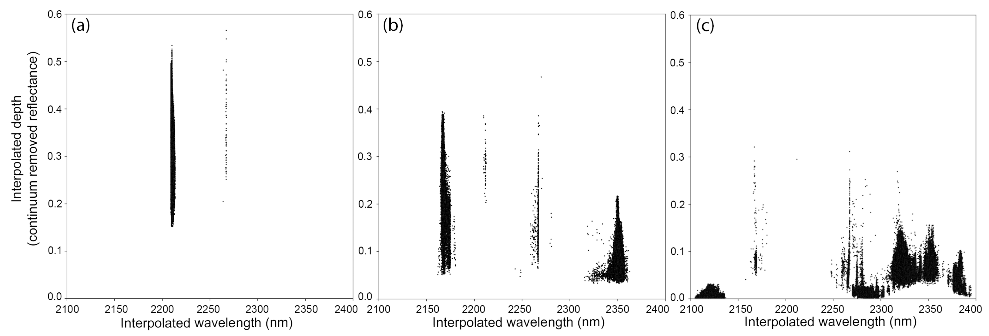
2.3. Wavelength Mapping
2.4. Summary Products
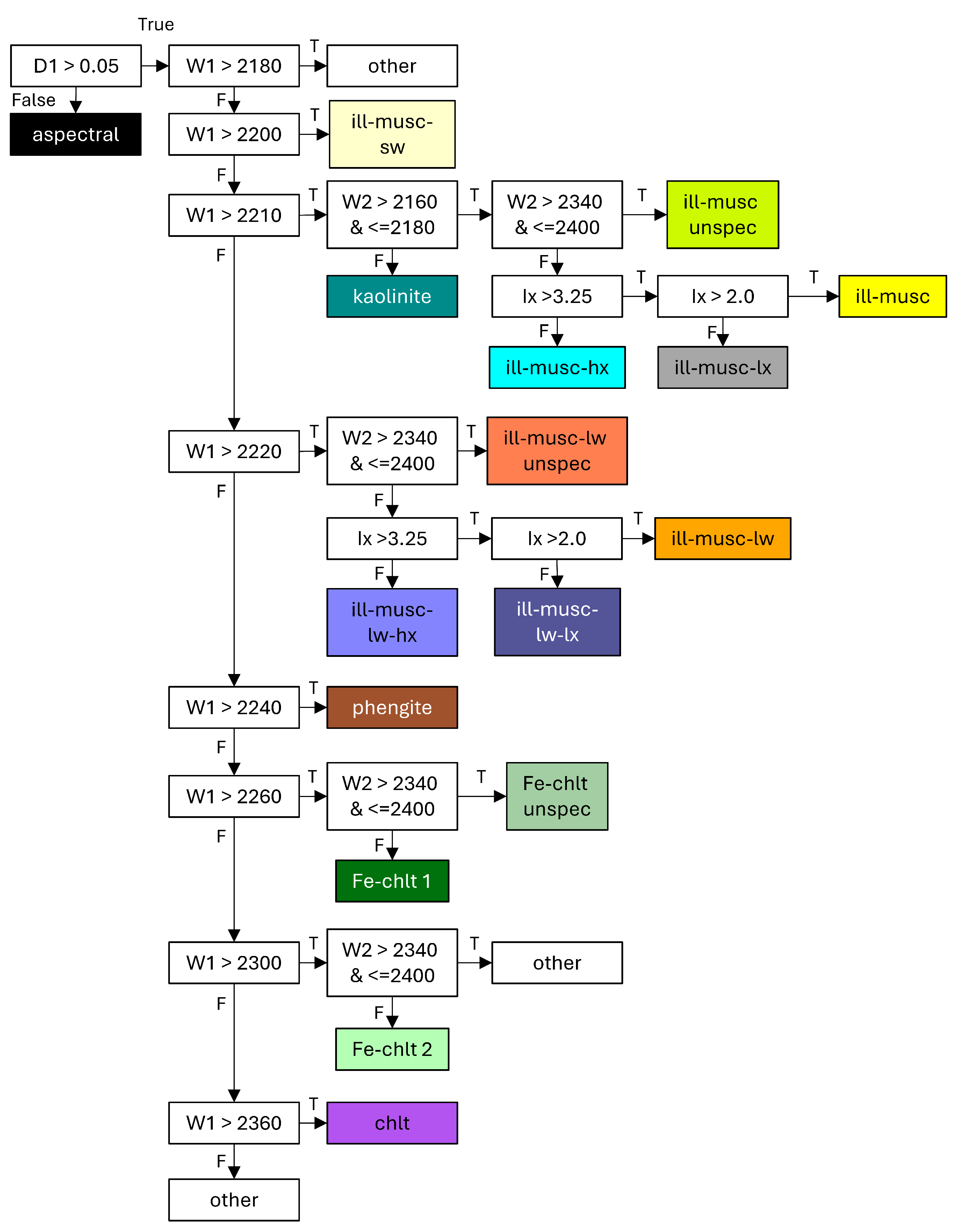
2.5. Decision Trees

| Decision Tree | Resulting Classified Image | Description |
|---|---|---|
| wave2100–2400_class | Classification based on depth of deepest and wavelength positions of first and second deepest absorption features in wavelength image between 2100 and 2400 nm (see Figure A2). | |
| albedo_class | Slicing of albedo image at thresholds: 0.25, 0.38 and 0.50 (see Figure A3). | |
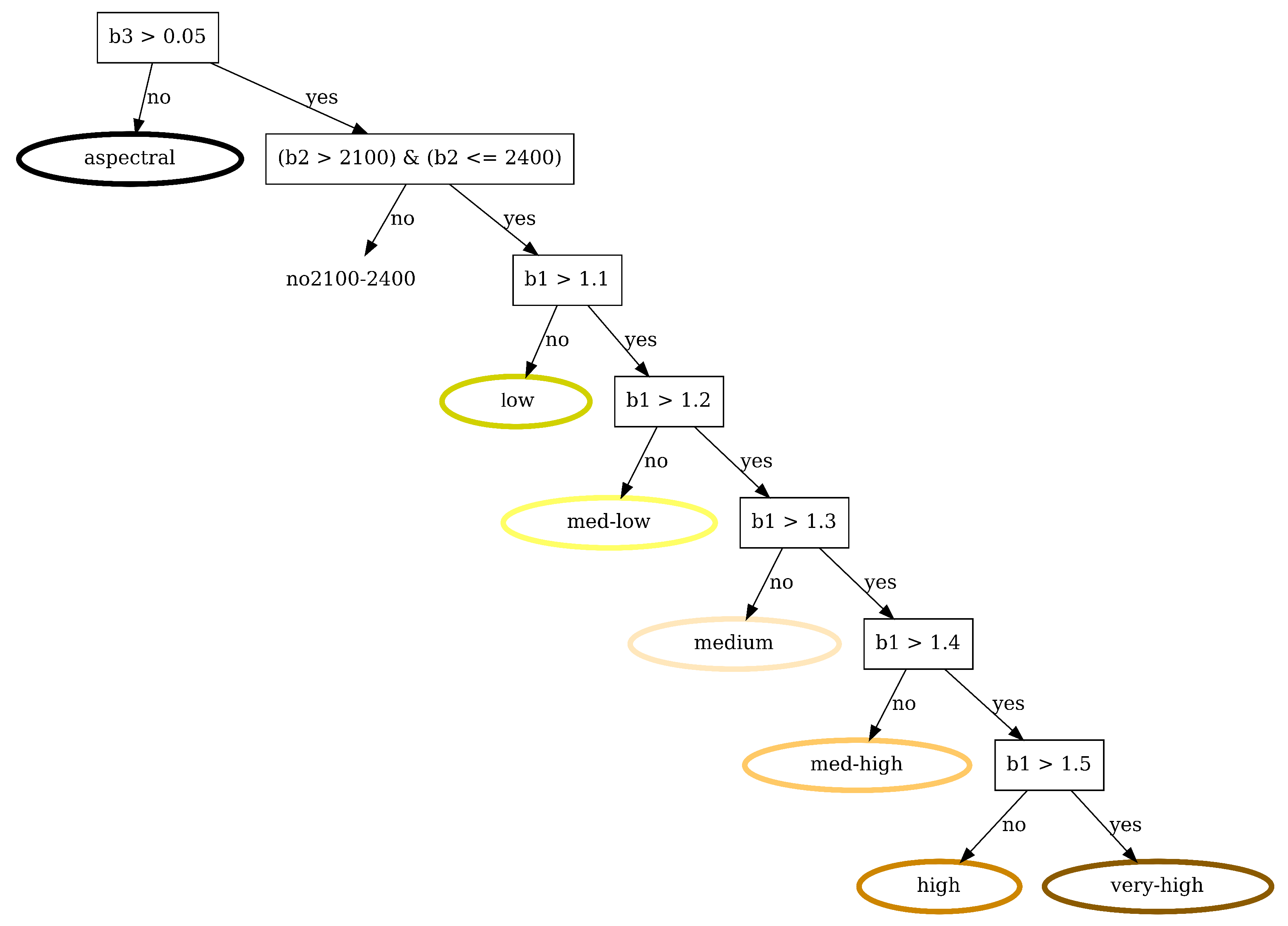
| fedrop_class | Slicing of ferrous drop (fedrop) image at thresholds: 1.1, 1.2, 1.3, 1.4 and 1.5 (see Figure A4). | |
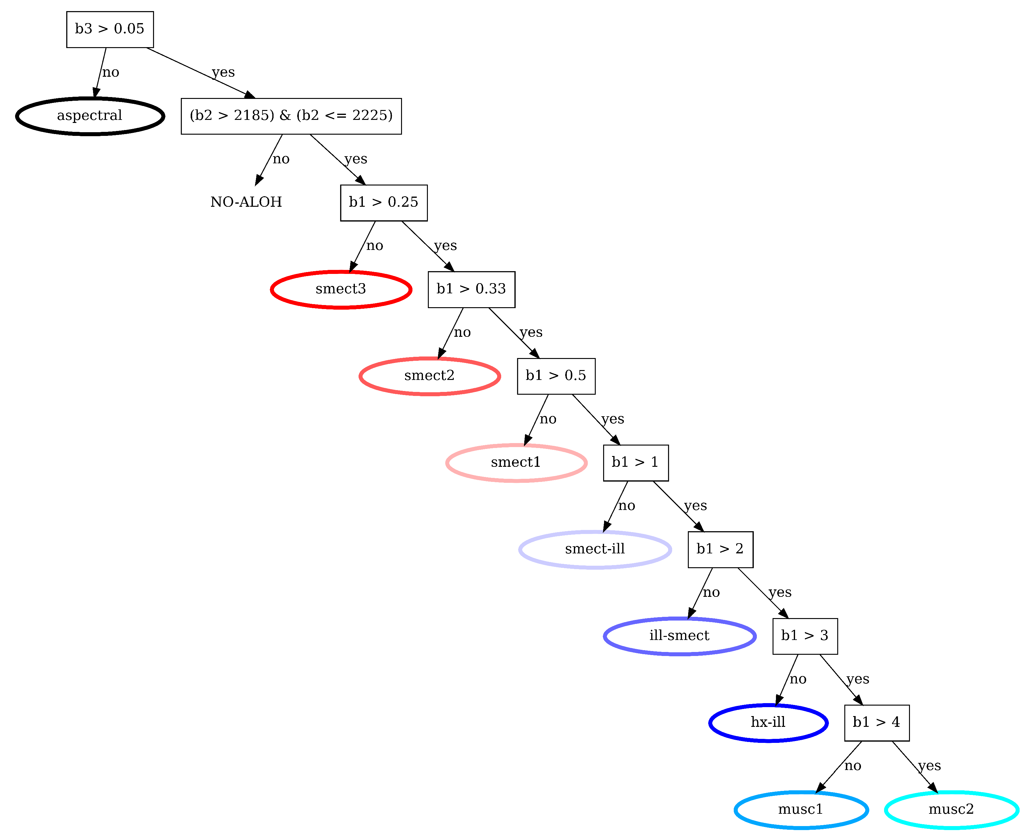
| illx_class | Slicing of illite crystallinity (illx) image at thresholds: 0.25, 0.33, 0.5, 1, 2, 3 and 4 (see Figure A5). | |
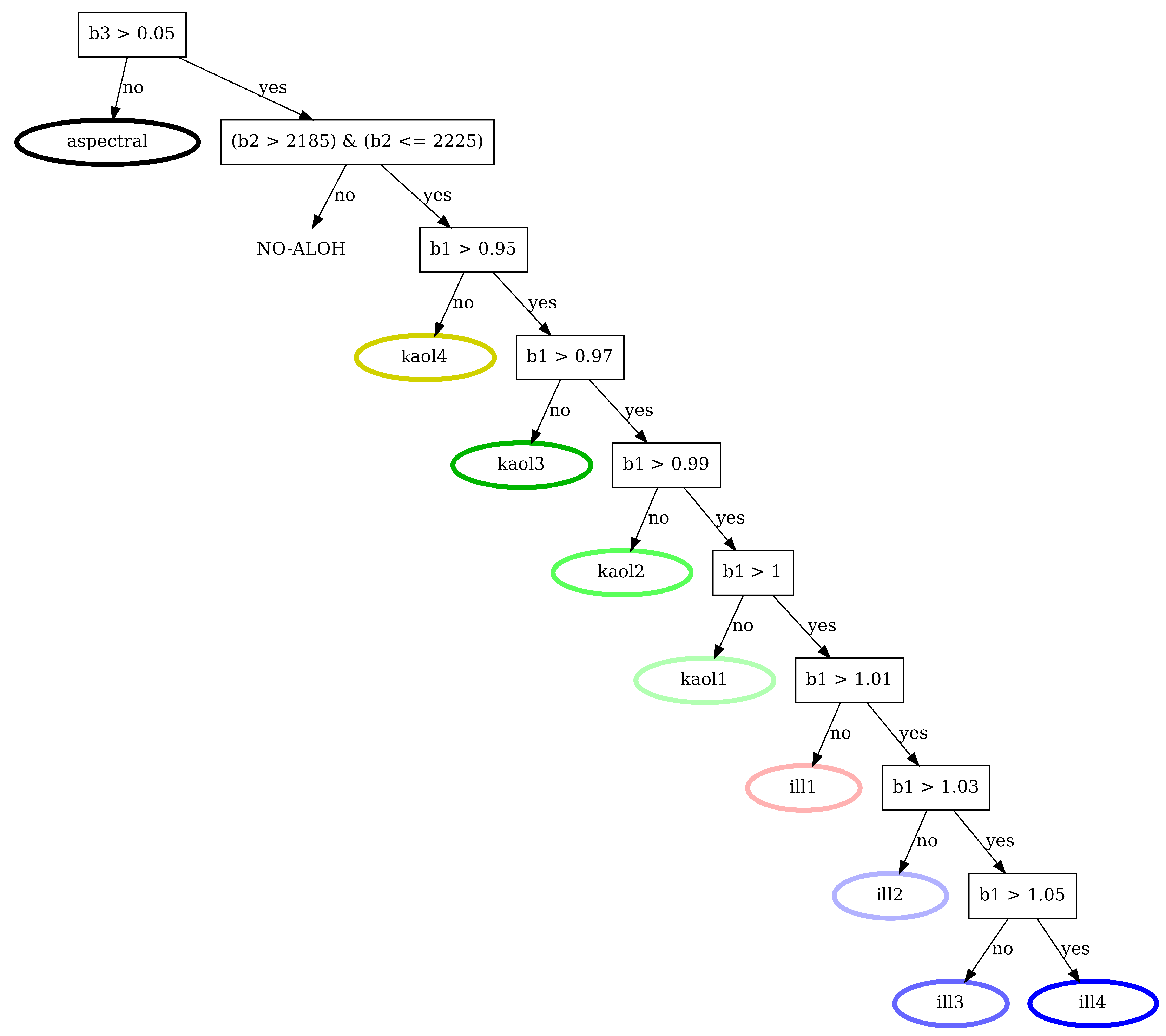
| illkaol_class | Slicing of illite over kaolinite (illkaol) image at thresholds: 0.95, 0.97, 0.99, 1.0, 1.01, 1.03 and 1.05 (see Figure A6). | |
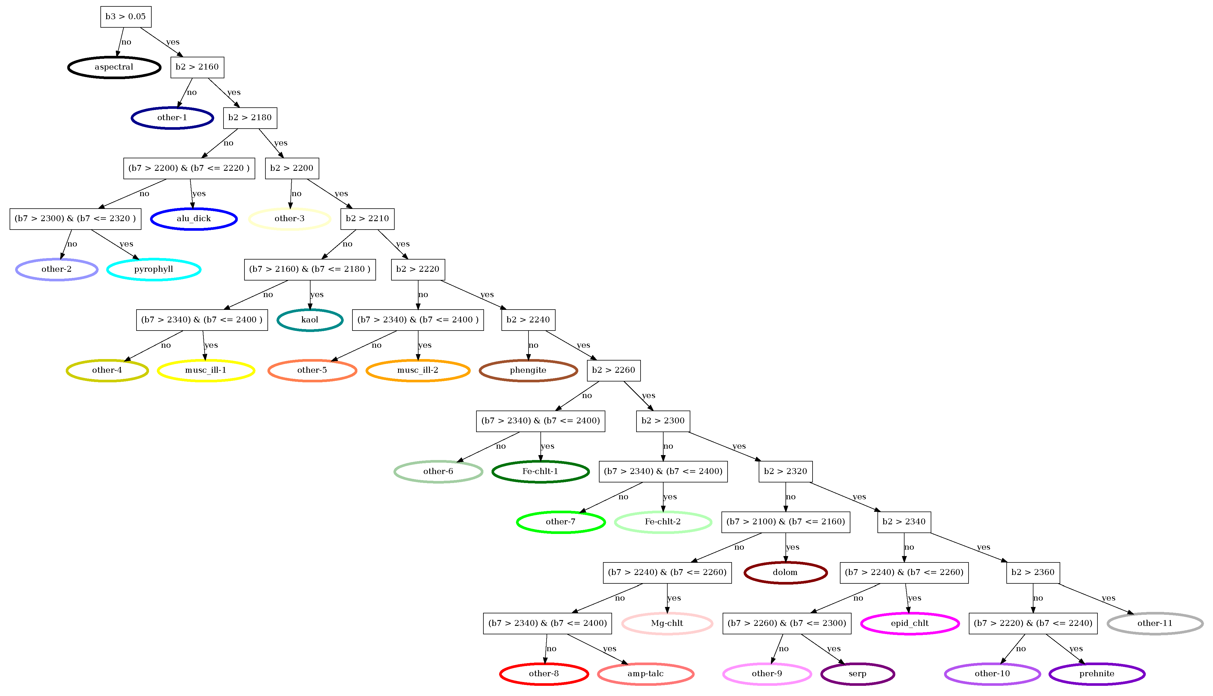
| mineral_map | Classification using depth and wavelength positions of deepest features in the wavelength images between 2100 and 2400 nm and the illite crystallinity image. Customized for the rock sample set in this study (see Figure 2). |
2.6. Mean Spectra of Classes
2.7. HypPy Software
2.8. Test Sample Set and Validation
3. Results
3.1. Exploratory Analyses
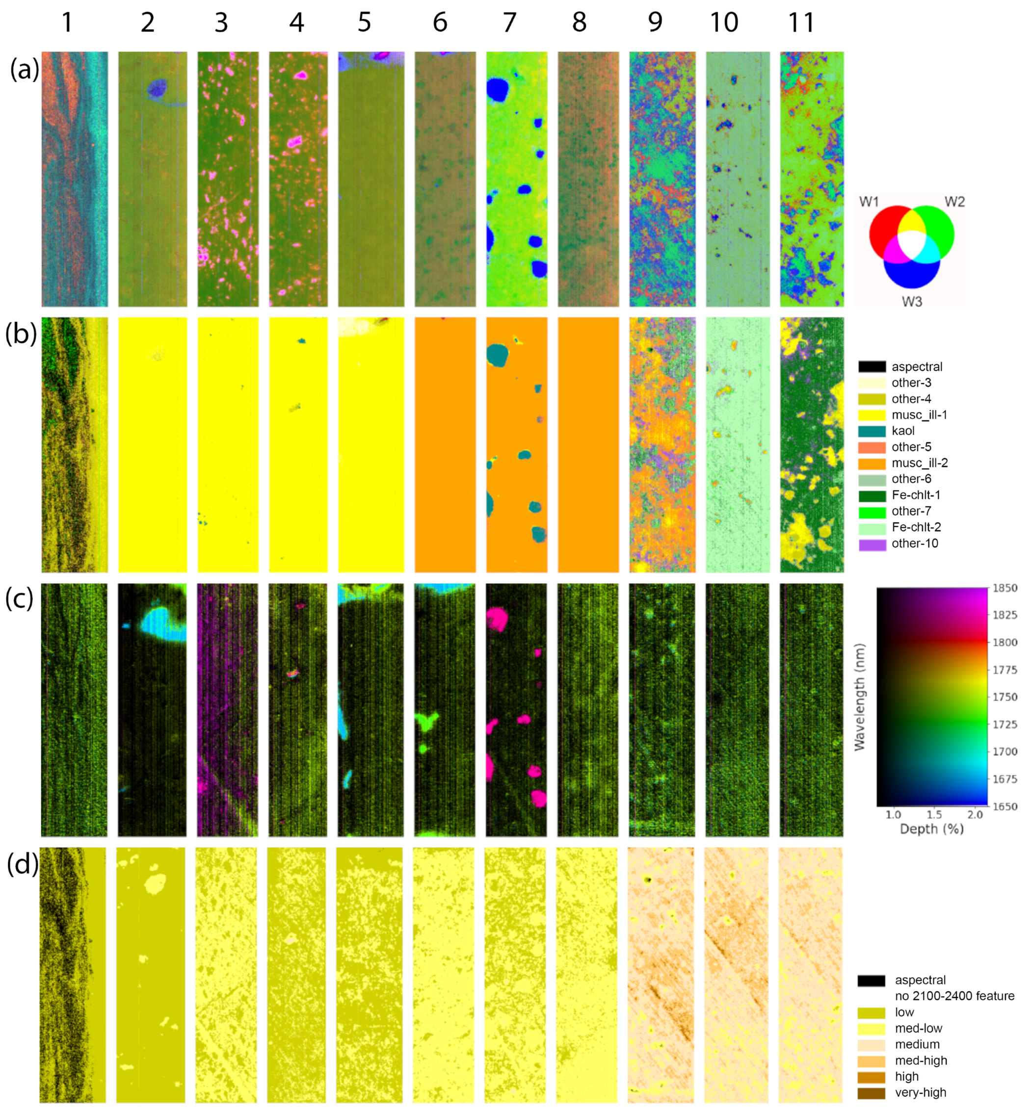

3.2. Mineral Maps and Comparison with Petrography
4. Discussion
4.1. Strengths
4.2. Weaknesses
4.3. Application
5. Conclusions
Author Contributions
Funding
Data Availability Statement
Acknowledgments
Conflicts of Interest
Appendix A. HypPy Command Line Syntax of Processing Steps
- 1.
- Conversion of uncalibrated radiance to reflectance image ($FILE-IN = manifest.xml file): > darkwhiteref.py -f -m $FILE-IN -o $FILE-OUT
- 2.
- Spatial–spectral filtering (mean7 = mean filtering by 2 spectral and 5 spatial neighbours): > median.py -f -i $FILE-IN -o $FILE-OUT -m mean7
- 3.
- Spectral math expression to create an optional mask file for dark background pixels (expression “S1.mean()>0.05” = mean pixel-spectrum is larger than 0.05; required for wavelength mapping command): > specmath.py -o $FILE-OUT -t int16 -e “S1.mean()>0.05” $FILE-IN
- 4.
- Creation of wavelength image (-w 2100 -W 2400 = wavelength range from 2100 to 2400; -m div = continuum removal by division; -n 3 = calculation of 3 deepest features): > minwavelength2.py -f -i $FILE-IN -o $FILE-OUT –mask $MASKFILE -w 2100 -W 2400 -m div -n 3 Creating a png image file of color composite of 1st, 2nd and 3rd deepest features in wavelength image (-R 0 -G 2 -B 4 = band numbers for the red, green and blue channels; -m SD = 2 standard deviations stretch mode): > tokml.py -i $FILE-IN -o $FILE-OUT -R 0 -G 2 -B 4 -m SD
- 6.
- Creation of wavelength map from wavelength image (-w 2100 -W 2400 = wavelength stretch range from 2100 to 2400; -d 0 -D 0 = standard depth stretch; -l = saves legend as .png): > wavemap.py -f -i $FILE-IN -o $FILE-OUT -w 2100 -W 2400 -d 0 -D 0 -l
- 7.
- Calculation of the summary products fedrop and illkaol (-u nan = input wavelength in nanometer; -l = creation of logfile): > otherindices.py -f -i $FILE-IN -o $FILE-OUT -u nan -l
- 8.
- Band math formula to calculate illx from wavelength images 2100–2400 nm and 1850–2100 nm (Expression: ‘i1[1] / i2[1]’ = ratio of band 1 in image 1 (wavelength image 2100–2400 nm, $FILE-IN1) over band 1 in image 2 (wavelength image 1850–2100 nm, $FILE-IN2)): > bandmath.py -o $FILE-OUT -e ‘i1[1] / i2[1]’ $FILE-IN1 $FILE-IN2
- 9.
- Spectral math expression to calculate albedo image, i.e., the mean spectrum of each pixel (‘S1.mean()’ = expression to calculate mean of spectrum): > specmath.py -o $FILE-OUT -e ‘S1.mean()’$FILE-IN
- 10.
- Band math formula to calculate illx from band ratio (expression: ‘i1(2178)/i1(2189)’ = ratio of bands 2187 over 2189 nm): > bandmath.py -o $FILE-OUT -e ‘i1(2178)/i1(2189)’ $FILE-IN
- 11.
- Spectral math expression to calculate Shannon entropy (expression: ‘(1-S1).entropy2()’= calculation of Shannon entropy): > specmath.py -o $FILE-OUT -e ‘(1-S1).entropy2()’ $FILE-IN
- 12.
- Classification using decision tree ($DT) of bands 0 (b2), 1 (b3) and 2 (b7) of wavelength image ($FILE-IN): > decisiontree.py -t $DT -o $FILE-OUT -b2 $FILE-IN 0 -b3 $FILE-IN 1 -b7 $FILE-IN 2
- 13.
- Creation of legend of classified file ($FILE-IN): > makelegend.py -i $FILE-IN
- 14.
- Calculation of mean spectra of all classes in class file ($CLASS-IN) from reflectance image ($FILE-IN) (-o $PLOT-OUT = plot of mean spectra; -l $SPECLIB = folder with ASCII mean spectra; -r $CLASSREPORT = report of class percentages in image): > classstats.py -i $FILE-IN -c $CLASS-IN -o $PLOT-OUT -l $SPECLIB -r $CLASSREPORT
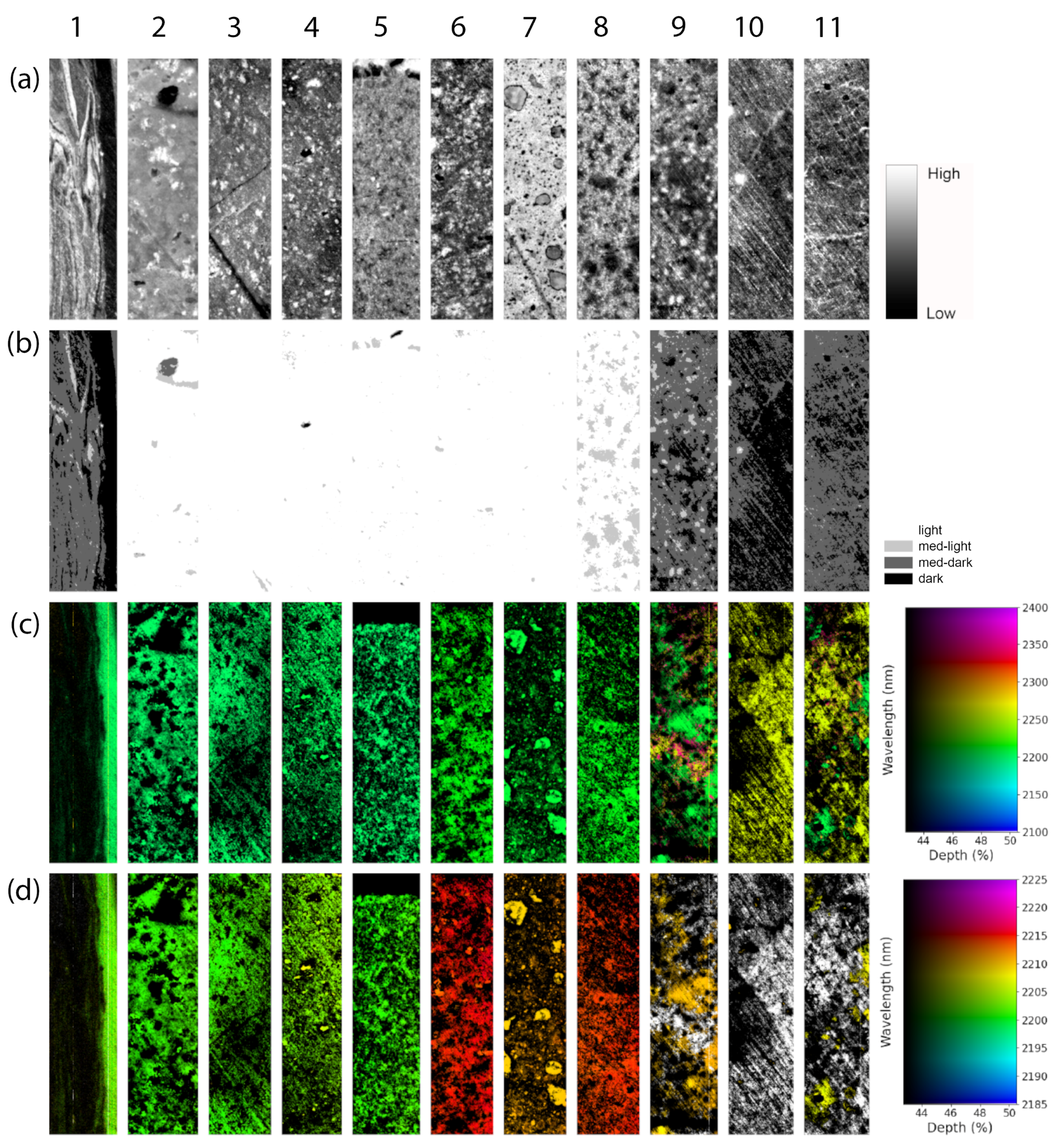
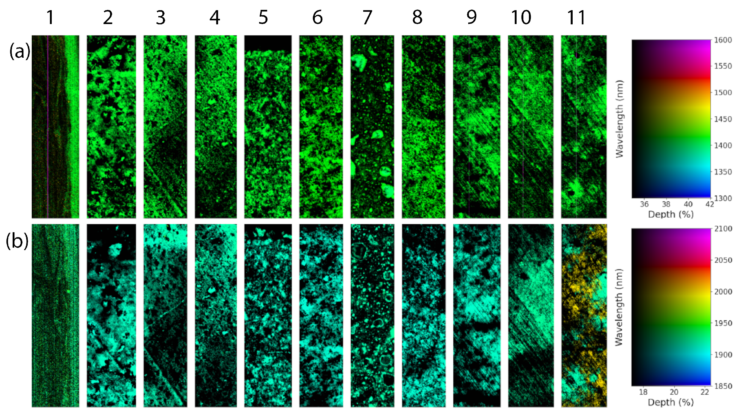
Appendix B. Wavelength Maps
Appendix C. Decision Trees

Appendix D. Micro-Photographs of Thin Sections
References
- Acosta, I.C.C.; Khodadadzadeh, M.; Tolosana-Delgado, R.; Gloaguen, R. Drill-core hyperspectral and geochemical data integration in a superpixel-based machine learning framework. IEEE J. Sel. Top. Appl. Earth Obs. Remote Sens. 2020, 13, 4214–4228. [Google Scholar] [CrossRef]
- Baissa, R.; Labbassi, K.; Launeau, P.; Gaudin, A.; Ouajhain, B. Using HySpex SWIR-320m hyperspectral data for the identification and mapping of minerals in hand specimens of carbonate rocks from the Ankloute Formation (Agadir Basin, Western Morocco). J. Afr. Earth Sci. 2011, 61, 1–9. [Google Scholar] [CrossRef]
- Dalm, M.; Buxton, M.; Van Ruitenbeek, F. Discriminating ore and waste in a porphyry copper deposit using short-wavelength infrared (SWIR) hyperspectral imagery. Miner. Eng. 2017, 105, 10–18. [Google Scholar] [CrossRef]
- Kruse, F. Identification and mapping of minerals in drill core using hyperspectral image analysis of infrared reflectance spectra. Int. J. Remote Sens. 1996, 17, 1623–1632. [Google Scholar] [CrossRef]
- Mathieu, M.; Roy, R.; Launeau, P.; Cathelineau, M.; Quirt, D. Alteration mapping on drill cores using a HySpex SWIR-320m hyperspectral camera: Application to the exploration of an unconformity-related uranium deposit (Saskatchewan, Canada). J. Geochem. Explor. 2017, 172, 71–88. [Google Scholar] [CrossRef]
- Turner, D.; Groat, L.A.; Rivard, B.; Belley, P.M. Reflectance spectroscopy and hyperspectral imaging of sapphire-bearing marble from the beluga occurrence, Baffin Island, Nunavut. Can. Mineral. 2017, 55, 787–797. [Google Scholar] [CrossRef]
- Van der Meer, F.D.; Van der Werff, H.M.; Van Ruitenbeek, F.J.; Hecker, C.A.; Bakker, W.H.; Noomen, M.F.; Van Der Meijde, M.; Carranza, E.J.M.; De Smeth, J.B.; Woldai, T. Multi-and hyperspectral geologic remote sensing: A review. Int. J. Appl. Earth Obs. Geoinf. 2012, 14, 112–128. [Google Scholar] [CrossRef]
- Clark, R.N. Spectroscopy of rocks and minerals, and principles of spectroscopy. In Manual of Remote Sensing; Rencz, A.N., Ed.; Remote Sensing for the Earth Sciences; John Wiley and Sons: New York, NY, USA, 1999; Volume 3, pp. 3–58. Available online: https://pubs.usgs.gov/publication/70196852 (accessed on 2 April 2025).
- Laukamp, C.; Rodger, A.; LeGras, M.; Lampinen, H.; Lau, I.C.; Pejcic, B.; Stromberg, J.; Francis, N.; Ramanaidou, E. Mineral physicochemistry underlying feature-based extraction of mineral abundance and composition from shortwave, mid and thermal infrared reflectance spectra. Minerals 2021, 11, 347. [Google Scholar] [CrossRef]
- Asadzadeh, S.; de Souza Filho, C.R. A review on spectral processing methods for geological remote sensing. Int. J. Appl. Earth Obs. Geoinf. 2016, 47, 69–90. [Google Scholar] [CrossRef]
- Kurz, T.H.; Buckley, S.J.; Howell, J.A. Close-range hyperspectral imaging for geological field studies: Workflow and methods. Int. J. Remote Sens. 2013, 34, 1798–1822. [Google Scholar] [CrossRef]
- Rodger, A.; Fabris, A.; Laukamp, C. Feature extraction and clustering of hyperspectral drill core measurements to assess potential lithological and alteration boundaries. Minerals 2021, 11, 136. [Google Scholar] [CrossRef]
- Wolfe, J.; Black, S. Hyperspectral Analytics in ENVI. 2018. Available online: https://www.spectroexpo.com/wp-content/uploads/2021/03/Hyperspectral_Whitepaper.pdf (accessed on 2 April 2025).
- Kleynhans, T.; Messinger, D.W.; Delaney, J.K. Towards automatic classification of diffuse reflectance image cubes from paintings collected with hyperspectral cameras. Microchem. J. 2020, 157, 104934. [Google Scholar] [CrossRef]
- Kruse, F.; Letkoff, A.; Boardmann, J.; Heidebrecht, K.; Shapiro, A.; Barloon, P.; Goetz, A. The spectral image processing system (SIPS)—Interactive visualization and analysis of imaging spectrometer data. Remote Sens. Environ. 1993, 44, 145–163. [Google Scholar] [CrossRef]
- Boardman, J.W.; Kruse, F.A. Analysis of imaging spectrometer data using n-dimensional geometry and a mixture-tuned matched filtering approach. IEEE Trans. Geosci. Remote Sens. 2011, 49, 4138–4152. [Google Scholar] [CrossRef]
- Bioucas-Dias, J.M.; Plaza, A.; Dobigeon, N.; Parente, M.; Du, Q.; Gader, P.; Chanussot, J. Hyperspectral unmixing overview: Geometrical, statistical, and sparse regression-based approaches. IEEE J. Sel. Top. Appl. Earth Obs. Remote Sens. 2012, 5, 354–379. [Google Scholar] [CrossRef]
- Paoletti, M.; Haut, J.; Plaza, J.; Plaza, A. Deep learning classifiers for hyperspectral imaging: A review. ISPRS J. Photogramm. Remote Sens. 2019, 158, 279–317. [Google Scholar] [CrossRef]
- Clark, R.N.; Swayze, G.A.; Livo, K.E.; Kokaly, R.F.; Sutley, S.J.; Dalton, J.B.; McDougal, R.R.; Gent, C.A. Imaging spectroscopy: Earth and planetary remote sensing with the USGS Tetracorder and expert systems. J. Geophys. Res. Planets 2003, 108, 5131. [Google Scholar] [CrossRef]
- Kokaly, R.F.; King, T.V.; Hoefen, T.M. Mapping the distribution of materials in hyperspectral data using the USGS Material Identification and Characterization Algorithm (MICA). In Proceedings of the 2011 IEEE International Geoscience and Remote Sensing Symposium, Vancouver, BC, Canada, 24–29 July 2011; pp. 1569–1572. [Google Scholar]
- Bakker, W.; van Ruitenbeek, F.; van der Werff, H.; Hecker, C.; Dijkstra, A.; van der Meer, F. Hyperspectral Python—HypPy. Algorithms 2024, 17, 337. [Google Scholar] [CrossRef]
- Thiele, S.T.; Lorenz, S.; Kirsch, M.; Acosta, I.C.C.; Tusa, L.; Herrmann, E.; Möckel, R.; Gloaguen, R. Multi-scale, multi-sensor data integration for automated 3-D geological mapping. Ore Geol. Rev. 2021, 136, 104252. [Google Scholar] [CrossRef]
- Acosta, I.C.C.; Khodadadzadeh, M.; Tusa, L.; Ghamisi, P.; Gloaguen, R. A Machine Learning Framework for Drill-Core Mineral Mapping Using Hyperspectral and High-Resolution Mineralogical Data Fusion. IEEE J. Sel. Top. Appl. Earth Obs. Remote Sens. 2019, 12, 4829–4842. [Google Scholar] [CrossRef]
- Lobo, A.; Garcia, E.; Barroso, G.; Martí, D.; Fernandez-Turiel, J.L.; Ibáñez-Insa, J. Machine Learning for Mineral Identification and Ore Estimation from Hyperspectral Imagery in Tin–Tungsten Deposits: Simulation under Indoor Conditions. Remote Sens. 2021, 13, 3258. [Google Scholar] [CrossRef]
- Trott, M.; Mooney, C.; Azad, S.; Sattarzadeh, S.; Bluemel, B.; Leybourne, M.; Layton-Matthews, D. Alteration assemblage characterization using machine learning applied to high-resolution drill-core images, hyperspectral data and geochemistry. Geochem. Explor. Environ. Anal. 2023, 23, geochem2023-032. [Google Scholar] [CrossRef]
- Thiele, S.; Kirsch, M.; Kamath, A.; Lorenz, S.; Kim, Y.; Gloaguen, R. Big data techniques for real-time hyperspectral core logging and mineralogical upscaling. In Proceedings of the 2024 International Conference on Machine Intelligence for GeoAnalytics and Remote Sensing (MIGARS), Wellington, New Zealand, 8–10 April 2024; pp. 1–3. [Google Scholar] [CrossRef]
- Hecker, C.; Van der Meijde, M.; Van Der Werff, H.; Van Der Meer, F.D. Assessing the influence of reference spectra on synthetic SAM classification results. IEEE Trans. Geosci. Remote Sens. 2008, 46, 4162–4172. [Google Scholar] [CrossRef]
- Van Ruitenbeek, F. High-Resolution, Laboratory Acquired Hyperspectral Images of Rock Samples from the Footwall of the Kangaroo Caves Cu-Zn Deposit, Pilbara, Western Australia; DANS Data Station Physical and Technical Sciences: The Hague, The Netherlands, 2024. [Google Scholar] [CrossRef]
- Hecker, C.; van Ruitenbeek, F.J.; van der Werff, H.M.; Bakker, W.H.; Hewson, R.D.; van der Meer, F.D. Spectral absorption feature analysis for finding ore: A tutorial on using the method in geological remote sensing. IEEE Geosci. Remote Sens. Mag. 2019, 7, 51–71. [Google Scholar] [CrossRef]
- Van Ruitenbeek, F.J.; Bakker, W.H.; van der Werff, H.M.; Zegers, T.E.; Oosthoek, J.H.; Omer, Z.A.; Marsh, S.H.; van der Meer, F.D. Mapping the wavelength position of deepest absorption features to explore mineral diversity in hyperspectral images. Planet. Space Sci. 2014, 101, 108–117. [Google Scholar] [CrossRef]
- Pineau, M.; Chauviré, B.; Rondeau, B. Near-infrared signature of hydrothermal opal: A case study of Icelandic silica sinters. Eur. J. Mineral. 2023, 35, 949–967. [Google Scholar] [CrossRef]
- Viviano, C.; Seelos, F.; Murchie, S.; Kahn, E.; Seelos, K.; Taylor, H.; Taylor, K.; Ehlmann, B.; Wiseman, S.; Mustard, J.; et al. Revised CRISM spectral parameters and summary products based on the currently detected mineral diversity on Mars. J. Geophys. Res. Planets 2014, 119, 1403–1431. [Google Scholar] [CrossRef]
- Pontual, S.; Merry, N.; Gamson, P. GMEX, Practical Applications Handbook; AusSpec International Pty. Ltd.: Arrowtown, New Zealand, 1997. [Google Scholar]
- Dalm, M.; Buxton, M.W.; van Ruitenbeek, F.J.; Voncken, J.H. Application of near-infrared spectroscopy to sensor based sorting of a porphyry copper ore. Miner. Eng. 2014, 58, 7–16. [Google Scholar] [CrossRef]
- Van Ruitenbeek, F.; Goseling, J.; Bakker, W.H.; Hein, K.A. Shannon entropy as an indicator for sorting processes in hydrothermal systems. Entropy 2020, 22, 656. [Google Scholar] [CrossRef]
- Safavian, S.R.; Landgrebe, D. A survey of decision tree classifier methodology. IEEE Trans. Syst. Man Cybern. 1991, 21, 660–674. [Google Scholar] [CrossRef]
- Qasim, M.; Khan, S.D. Detection and relative quantification of Neodymium in Sillai Patti Carbonatite using decision tree classification of the Hyperspectral Data. Sensors 2022, 22, 7537. [Google Scholar] [CrossRef]
- Van Ruitenbeek, F.; van der Werff, H.; Hein, K.; van der Meer, F. Detection of pre-defined boundaries between hydrothermal alteration zones using rotation-variant template matching. Comput. Geosci. 2008, 34, 1815–1826. [Google Scholar] [CrossRef]
- Van Hinsberg, C. An Integrated Study of Hydrothermal White Mica in the Footwall of the Kangaroo Caves VMS Deposit, Western Australia. Master’s Thesis, Utrecht University, Utrecht, The Netherlands, 2010. Available online: https://studenttheses.uu.nl/bitstream/handle/20.500.12932/5473/Thesis.pdf?sequence=1 (accessed on 2 April 2025).
- Van Ruitenbeek, F.; Hein, K. Rock Sample Data from the Footwall of the Kangaroo Caves Cu-Zn Deposit, Pilbara, Western Australia; DANS Data Station Physical and Technical Sciences: The Hague, The Netherlands, 2019. [Google Scholar] [CrossRef]
- Kokaly, R.; Clark, R.; Swayze, G.; Livo, K.; Hoefen, T.; Pearson, N.; Wise, R.; Benzel, W.; Lowers, H.; Driscoll, R.; et al. USGS Spectral Library Version 7 Data: US Geological Survey Data Release; United States Geological Survey (USGS): Reston, VA, USA, 2017; Volume 61. [Google Scholar] [CrossRef]
- Hunt, G.R. Spectral signatures of particulate minerals in the visible and near infrared. Geophysics 1977, 42, 501–513. [Google Scholar] [CrossRef]
- Duke, E. Near infrared spectra of muscovite, Tschermak substitution, and metamorphic reaction progress: Implications for remote sensing. Geology 1994, 22, 621–624. [Google Scholar] [CrossRef]
- Van Ruitenbeek, F.; van der Werff, H.; Bakker, W.; van der Meer, F.; Hein, K. Measuring rock microstructure in hyperspectral mineral maps. Remote Sens. Environ. 2019, 220, 94–109. [Google Scholar] [CrossRef]
- Savitri, K. P Spectral Analysis for Geothermal Exploration: A Method Investigation to Bring the Technology Closer to Geothermal Community. Ph.D. Thesis, University of Twente, Enschede, The Netherlands, 2024. Available online: https://research.utwente.nl/en/publications/spectral-analysis-for-geothermal-exploration-a-method-investigati (accessed on 2 April 2025).
- Martynenko, S.; Tuisku, P.; van Ruitenbeek, F.; Hein, K. High-resolution short-wave infrared hyperspectral characterization of alteration at the Sadiola Hill gold deposit, Mali, Western Africa. In Proceedings of the 15th Biennial Meeting of the Society for Geology Applied to Mineral Deposits: Life with Ore Deposits on Earth, Glasgow, UK, 27–30 August 2019; University of Glasgow: Glasgow, UK, 2019; p. 1325. Available online: https://ris.utwente.nl/ws/portalfiles/portal/138697676/283_SGA_Martynenko_et_al_2019_Final.pdf (accessed on 2 April 2025).

| Name | Description | Interpretation |
|---|---|---|
| Albedo | Mean reflectance value of all bands in a pixel spectrum. | Brightness. |
| Ferrous drop (fedrop) | Ratio of reflectance bands at 1600 over 1310 nm [33]. | Indication of ferrous iron in minerals, e.g., illite and carbonates. High values indicate abundant ferrous iron in the mineral. |
| Illite crystallinity (illx) | Ratio of the depths of deepest features between 2100–2400 and 1850–2100 nm, i.e., the depths of the Al-OH feature and water features of smectite–illite–muscovite minerals [33]. | Indication of the degree of ordering of the mineral, e.g., [34]; High values indicate relatively high degrees of ordering. |
| Illite–kaolinite (illkaol) | Ratio of reflectance bands at 2164 over 2180 nm. The 2164 nm band is positioned at the second deepest feature of the doublet feature of kaolinite and the 2180 nm band is positioned at the high between the double feature [33]. | Indication for the relative amounts of illite (high values) and kaolinite (low values). Note that the values are affected by the type of kaolinite in the rock and the center wavelengths of the bands of the hyperspectral camera used. |
| Shannon entropy | Measure from information theory: | It measures the deviation from a flat horizontal spectrum. A flat spectrum results in highest Shannon entropy values. Spectra with few but deep features produce low values. |
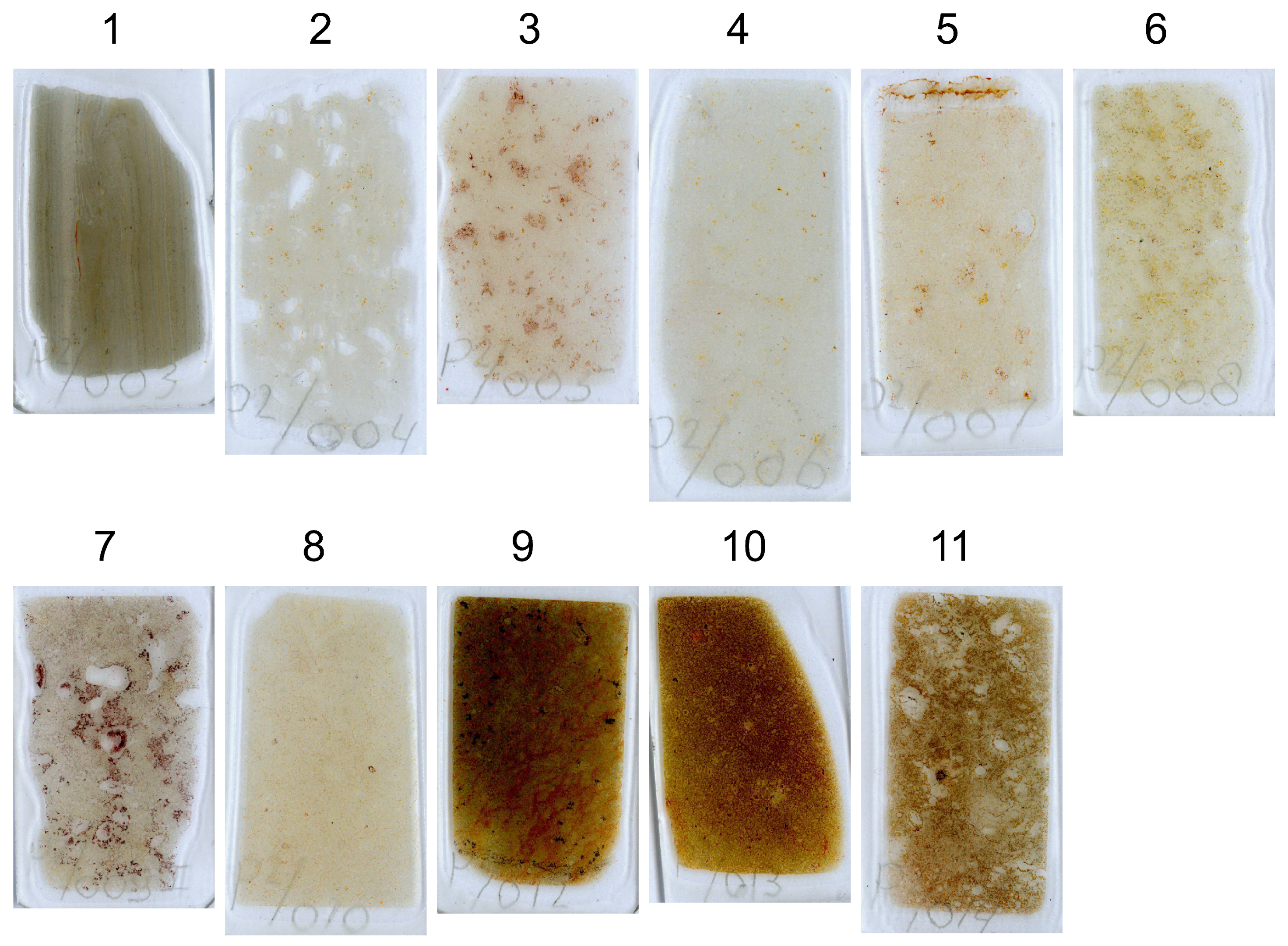
| ID | Sample | Description |
|---|---|---|
| 1 | P2003 | Weakly sericite altered and silicified muddy chert. |
| 2 | P2004 | Deuterically altered, silicified, seriticized (Al-rich), xenocrystic phenocrystic andesite. |
| 3 | P2005 | Deuterically altered, silicified, seriticized (Al-rich), phenocrystic andesite. |
| 4 | P2006 | Deuterically altered, silicified, seriticized (Al-rich), weakly phenocrystic andesite. |
| 5 | P2007 | Deuterically altered, silicified, seriticized (Al-rich), weakly phenocrystic quenched andesite. |
| 6 | P2008 | Deuterically altered, silicified, seriticized (Al-poor), weakly phenocrystic andesite. |
| 7 | P2009a | Deuterically altered, silicified, seriticized (Al-poor), weakly xenocrystic amygdaloidal basalt. Contains aproximately 15% kaolinite in amygdales. |
| 8 | P2010 | Deuterically altered, silicified, seriticized (Al-poor), weakly xenocrystic weakly amygdaloidal basalt. |
| 9 | P2012 | Deuterically altered, silicified, ferruginous, chloritised basalt. |
| 10 | P2013 | Deuterically altered, silicified, ferruginous, chloritised (pyroxene-bearing) basalt. |
| 11 | P2014 | Deuterically altered, silicified, chloritised amygdaloidal andesite. |
| Sample Number | Mineral Map Classes 1 | Percentage Image Pixels 2 | Minerals Identified Using Petrography |
|---|---|---|---|
| (1) P2003 | ill-musc unspec | 45.5 | Quartz, hematite, goethite, rutile, sericite |
| aspectral | 32.2 | ||
| ill-musc-lw unspec | 6.7 | ||
| other | 6.1 | ||
| ill-musc | 5.0 | ||
| (2) P2004 | ill-musc | 92.2 | Quartz, sericite, goethite |
| ill-musc-lx | 4.0 | ||
| ill-musc-hx | 3.3 | ||
| (3) P2005 | ill-musc | 92.9 | Quartz, sericite, goethite |
| ill-musc-hx | 3.8 | ||
| ill-musc-lx | 2.7 | ||
| (4) P2006 | ill-musc-lx | 87.2 | Quartz, sericite, goethite |
| ill-musc | 12.1 | ||
| (5) P2007 | ill-musc | 92.7 | Quartz, sericite, goethite |
| ill-musc-lx | 3.5 | ||
| ill-musc-sw | 2.9 | ||
| (6) P2008 | ill-musc-lw | 95.7 | Quartz, sericite, goethite |
| ill-musc-lw-hx | 2.1 | ||
| (7) P2009a | ill-musc-lw-hx | 45.1 | Quartz, sericite, goethite, accessory chlorite |
| ill-musc-lw | 44.4 | ||
| kaolinite | 6.7 | ||
| (8) P2010 | ill-musc-lw | 99.1 | Quartz, sericite, goethite, hematite, accessory chlorite |
| (9) P2012 | ill-musc-lw-lx | 21.8 | Quartz, goethite, chlorite, accessory sericite |
| ill-musc-lw unspec | 21.5 | ||
| chlt | 14.1 | ||
| ill-musc-lx | 9.3 | ||
| Fe-chlt | 8.0 | ||
| Fe-chlt unspec | 6.3 | ||
| ill-musc unspec | 6.3 | ||
| other | 5.0 | ||
| (10) P2013 | Fe-chlt | 89.9 | Quartz, goethite, chlorite |
| (11) P2014 | Fe-chlt | 66.2 | Quartz, chlorite, goethite |
| ill-musc unspec | 9.0 | ||
| chlt | 8.5 | ||
| ill-musc | 6.9 | ||
| Fe-chlt unspec | 5.5 | ||
| ill-musc-lx | 3.1 |
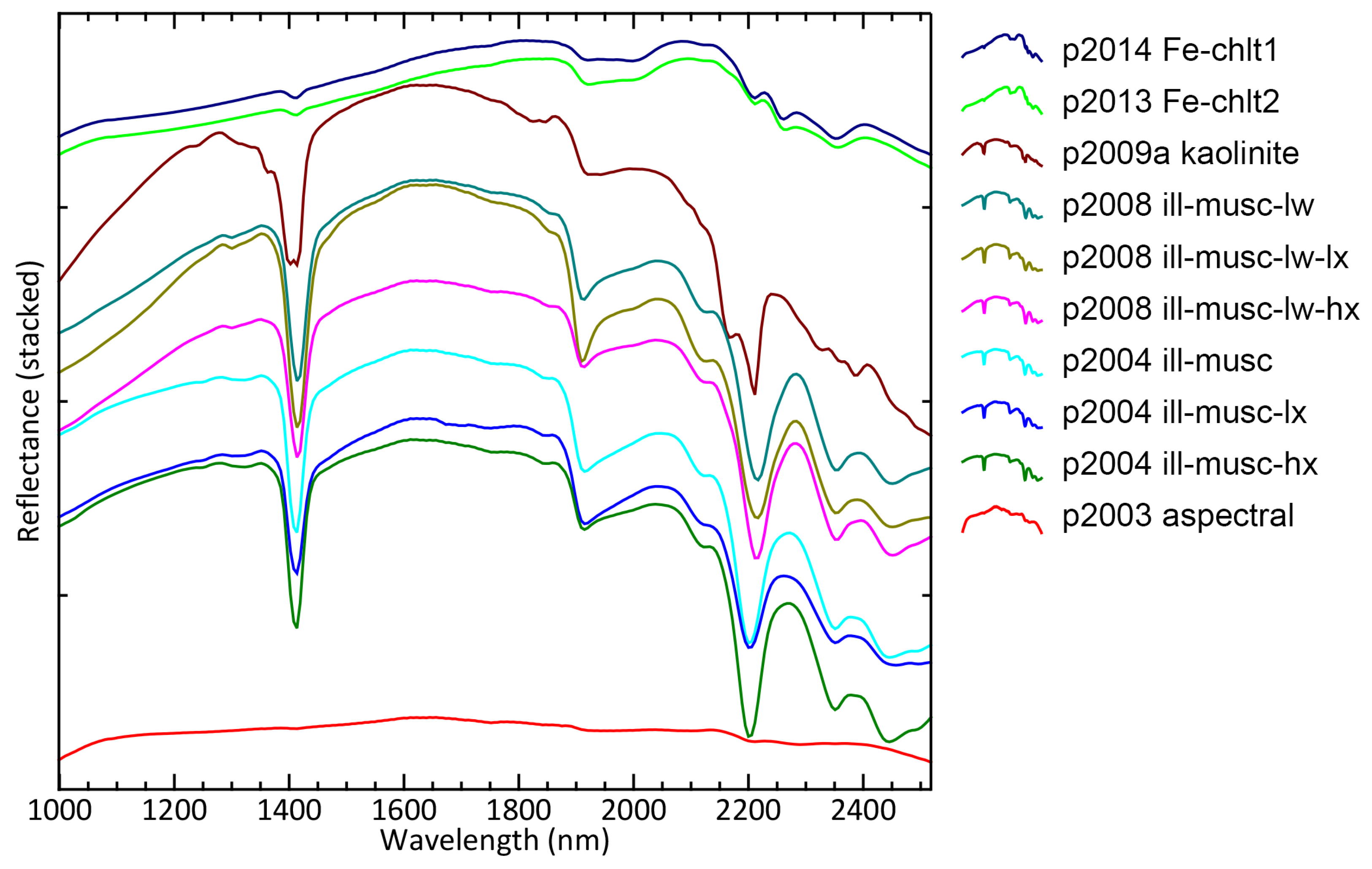
| Class | Count | Reference Spectrum |
|---|---|---|
| ill-musc-sw | 2 | Muscovite_GDS113_Ruby; Muscovite_GDS113a_Ruby |
| phengite | 2 | Illite_GDS4.2_Marblehead; Illite_GDS4_Marblehead |
| epid/chlt | 5 | Chlorite_HS179.1B; Chlorite_HS179.2B; Chlorite_HS179.3B; Chlorite_HS179.4B; Chlorite_HS179.6 |
| ill-musc-hx | 3 | Muscovite_HS146.1B; Muscovite_HS146.3B; Muscovite_HS146.4B |
| ill-musc-lx | 2 | Illite_IMt-1.a; Illite_IMt-1.b_lt2um |
| ill-musc-lw-hx | 2 | Muscovite_GDS116_Tanzania; Muscovite_GDS116a_Tanzania |
| kaolinite | 3 | Kaolinite_CM9; Kaolinite_KGa-1_(wxl); Kaolinite_KGa-2_(pxl) |
Disclaimer/Publisher’s Note: The statements, opinions and data contained in all publications are solely those of the individual author(s) and contributor(s) and not of MDPI and/or the editor(s). MDPI and/or the editor(s) disclaim responsibility for any injury to people or property resulting from any ideas, methods, instructions or products referred to in the content. |
© 2025 by the authors. Licensee MDPI, Basel, Switzerland. This article is an open access article distributed under the terms and conditions of the Creative Commons Attribution (CC BY) license (https://creativecommons.org/licenses/by/4.0/).
Share and Cite
van Ruitenbeek, F.J.A.; Bakker, W.H.; van der Werff, H.M.A.; Hecker, C.A.; Hein, K.A.A.; van Eijndthoven, W. A Knowledge-Based Strategy for Interpretation of SWIR Hyperspectral Images of Rocks. Remote Sens. 2025, 17, 2555. https://doi.org/10.3390/rs17152555
van Ruitenbeek FJA, Bakker WH, van der Werff HMA, Hecker CA, Hein KAA, van Eijndthoven W. A Knowledge-Based Strategy for Interpretation of SWIR Hyperspectral Images of Rocks. Remote Sensing. 2025; 17(15):2555. https://doi.org/10.3390/rs17152555
Chicago/Turabian Stylevan Ruitenbeek, Frank J. A., Wim H. Bakker, Harald M. A. van der Werff, Christoph A. Hecker, Kim A. A. Hein, and Wijnand van Eijndthoven. 2025. "A Knowledge-Based Strategy for Interpretation of SWIR Hyperspectral Images of Rocks" Remote Sensing 17, no. 15: 2555. https://doi.org/10.3390/rs17152555
APA Stylevan Ruitenbeek, F. J. A., Bakker, W. H., van der Werff, H. M. A., Hecker, C. A., Hein, K. A. A., & van Eijndthoven, W. (2025). A Knowledge-Based Strategy for Interpretation of SWIR Hyperspectral Images of Rocks. Remote Sensing, 17(15), 2555. https://doi.org/10.3390/rs17152555