Spatiotemporal Characteristics of and Factors Influencing CO₂ Concentration During 2010–2023 in China

Abstract

Human activities at unprecedented levels have exacerbated the greenhouse effect and escalated the frequency of extreme weather. In response, the Chinese government has pledged to reach “carbon peak” by 2030 and achieve “carbon neutrality” by 2060. Leveraging the GOSAT L3 and L4B CO₂ datasets, this study investigated the spatiotemporal and vertical characteristics of atmospheric carbon dioxide (CO₂) concentration across China, alongside quantifying the relative importance of key influencing factors. The results show that there is a distinct regional disparity in CO₂ column concentration, with eastern China having a higher concentration level (406.85 × 10⁻⁶) than the western regions (400.92 × 10⁻⁶). Vertically, the concentration of CO₂ (390–420 × 10⁻⁶) reaches its peak at the near-surface layer (975 hPa) and then decreases with increasing altitude. High values of CO₂ levels in the mid-lower layer are concentrated in eastern China, while those in the upper layer are mainly located in southern China. In addition, CO₂ concentration shows seasonal variations, with the highest concentration occurring in spring (406.39 × 10⁻⁶) and the lowest in summer. Biospheric emissions and fossil fuel combustion emerge as the two most significant factors affecting CO₂ variation, with relative importance of 24% and 22%, respectively.

1. Introduction

Since the pre-industrial era (1850–1900), global greenhouse gas (GHG) emissions have risen steadily, driving a sustained increase in global mean surface temperature. Notably, the average global surface temperature over the period 2011–2020 was approximately 1.1 °C warmer than the pre-industrial baseline, highlighting the tangible climatic impacts of cumulative emissions [1] that have led to a marked rise in the frequency of extreme weather and climate events. As one of the significant GHGs, CO₂ continuously affects the human living environment and global climate [2]. In September 2020, China set the “dual carbon” goals, aiming to achieve “carbon peak” by 2030 and “carbon neutrality” by 2060 [3]. Therefore, accurate monitoring of the spatiotemporal variations in CO₂ concentration, coupled with quantification of the relative importance of influencing factors, is crucial for assessing the effectiveness of carbon mitigation efforts and formulating carbon reduction strategies.

Ground-based greenhouse gas observations can provide accurate, real-time measurements of atmospheric CO₂ concentrations. However, ground-based observations are subjected to inherent limitations. On one hand, challenges occur in characterizing CO₂ concentrations at regional and global scales, as well as tracking changes in the total atmospheric CO₂ burden [4]. On the other hand, the distribution of existing ground stations is sparse and highly uneven from a global perspective, leading to significant uncertainties in the derived CO₂ concentration [5,6]. Advances in space technology and remote sensing science have enabled satellite-based observations to reduce uncertainties in CO₂ concentration or flux estimations. Satellites can monitor atmospheric CO₂ in a more comprehensive and relatively stable manner, and have become an increasingly important tool for atmospheric CO₂ monitoring [7,8,9,10,11].

Numerous investigations have harnessed satellite-derived datasets to characterize the spatiotemporal dynamics of atmospheric CO₂ concentrations at both global and regional scales. Li et al. reconstructed a globally consistent, high-spatiotemporal-resolution dataset of CO₂ concentration through the integration of Orbiting Carbon Observatory 2 (OCO-2) satellite observations with data from eight influencing factors (e.g., meteorology and vegetation) [12]. The results revealed a distinct year-on-year rise in global CO₂ concentrations during 2014–2018, with the upward trend primarily concentrated in economically developed coastal regions. Yao et al. used Greenhouse Gases Observing Satellite (GOSAT) data to characterize the spatial patterns of atmospheric CO₂ across global terrestrial regions from 2010 to 2020 [13]. Their analysis revealed higher CO₂ concentrations in eastern Asia, central Africa, and southern North America, with pronounced peaks observed in tropical northern latitudes and mid-to-high latitudes of the Northern Hemisphere. Yin et al. investigated the influence of Australian climatic conditions on CO₂ spatiotemporal distributions using 2009–2016 GOSAT data. Their analysis revealed that sea surface temperature, precipitation, vegetation, ENSO events, oceanic chemical processes, and bushfires directly or indirectly modulated regional CO₂ variations [14]. Imasu et al. examined diurnal and seasonal CO₂ patterns across urban, suburban, and rural Japan based on extensive ground-based observations. They demonstrated urban winter midnight concentrations peaked during morning hours, while suburban maxima occurred at night and minima occurred in the daytime in summer, which was attributed to vegetation respiration and photosynthesis [15]. Deng et al. used GOSAT satellite data to analyze the spatiotemporal variation in atmospheric CO₂ across China from 2010 to 2016 [16]. Their findings revealed a distinct annual upward trend in CO₂ concentrations, with higher values concentrated in the Zhejiang–Jiangsu–Anhui region, the Beijing–Tianjin–Hebei region, and the Hunan–Hubei–Henan–Shanxi region. Lv et al. employed an integrated methodology combining GOSAT satellite observations with Kriging interpolation and characterized the spatiotemporal dynamics of atmospheric CO₂ concentrations across China during 2009–2016 [17]. The analysis revealed distinct seasonal patterns, whereby nationwide CO₂ concentrations peak in spring and reach their nadir in summer. Lv et al. examined the spatiotemporal distribution of CO₂ concentrations in China’s Yellow River Basin from 2013 to 2022 using OCO-2 and GOSAT satellite data [18]. The results showed that the highest CO₂ concentration occurred in the basin’s central region, exhibiting a peak in May and a nadir in August. Notably, comprehensive analysis of the long-term spatiotemporal distribution of atmospheric CO₂ concentrations over China from 2010 to 2023 based on satellite-derived observations remains scarce in existing research.

For the vertical distribution characteristics of CO₂, Gao et al. analyzed variations in CO₂ at heights of 30, 65, and 110 m during summer in Nanjing using ground-based observational data [19]. Their results revealed a discernible vertical gradient of CO₂ concentrations within the main urban area, with near-surface levels at 30 m significantly influenced by anthropogenic activities. Liu et al. investigated diurnal and monthly variations in CO₂ concentrations across varied heights (i.e., 8, 16, 47, 80, 140, 200 and 280 m) in urban Beijing, utilizing turbulence observation data from the Beijing Tower [20]. Their results demonstrated that CO₂ concentrations consistently decreased with increasing altitude, with all observational levels exhibiting significant diurnal cycles. Vertically, winter months showed the greatest diurnal concentration variability, while summer displayed the most pronounced inter-level concentration variations. Sun et al. utilized a Raman lidar system to measure vertical CO₂ distributions in the lower troposphere (below 2 km) over the western suburbs of Hefei from July 2014 to December 2015 [21]. The atmospheric vertical profile indicated decreasing CO₂ concentrations with increasing altitude throughout the lower troposphere. Pronounced variability occurred near the surface (<150 m), while concentrations stabilized within the 300–700 m altitude range. It can be seen that existing studies on CO₂ vertical distribution characteristics primarily relied on ground-based or instrumental observations rather than satellite data, with limited information on spatiotemporal characteristics for different vertical layers and/or comprehensive vertical profiles of whole atmospheric columns. Furthermore, most studies have focused only on individual cities. Therefore, comprehensive analyses at the national scale across China remain notably scarce.

Anthropogenic and natural CO₂ emissions, alongside meteorological conditions, are recognized as key drivers of CO₂ levels and trends [22,23,24]. Prior research has investigated how these factors influence CO₂ variability by utilizing statistical approaches (e.g., correlation analysis and multiple regression). For example, Mustafa et al. employed simple correlation analysis to dissect the determinants CO₂ concentrations across Asia, indicating that monsoon dynamics and land-use patterns served as key impact factors [25]. Lv et al. found that vegetation change, rather than anthropogenic emissions, is the dominant driver of temporal variation in atmospheric CO₂ concentrations across China, combining simple correlation and partial correlation analysis [17]. Zhu et al. utilized a multi-scale geographically weighted regression model to quantify the impacts of environmental variables on regional CO₂ concentrations across China [26]. Their findings demonstrated that carbon emissions exerted a greater impact on CO₂ levels than climate change or vegetation cover, while atmospheric circulation played a moderate role in shaping concentration dynamics. However, the aforementioned studies did not comprehensively analyze the relative contributions of these factors to CO₂ variability or the key controlling mechanisms, thereby limiting the capacity to elucidate the underlying processes governing CO₂ distribution and inform targeted mitigation strategies.

To deepen the understanding of long-term spatiotemporal variations in CO₂ and key factors influencing these across China, this study characterized the spatiotemporal patterns of CO₂ concentrations across China from 2010 to 2023 using the Kriging interpolation method based on GOSAT satellite data. Additionally, correlation analysis and random forest methods were employed to identify the key factors influencing CO₂ concentration changes. This study extends the research timeframe and combines correlation analysis with random forest modeling to quantify the relative importance of factors influencing CO₂ levels. Note that this study separately evaluated the impacts of CO₂ fluxes from specific emission categories on atmospheric CO₂ concentrations, unlike previous studies that typically analyzed the relative importance of CO₂ emission by aggregating all emissions as a single factor [26]. Furthermore, existing research in China has provided limited discussion on vertical spatiotemporal distribution characteristics of CO₂, with most analyses relying on instrumental observation data in localized areas. We conducted an in-depth analysis of the spatiotemporal distribution characteristics of CO₂ concentration at different vertical layers.

2. Data and Methodology

2.1. Data

The spatiotemporal and vertical distribution of atmospheric CO₂ over China was characterized using level 3 (L3) and level 4B (L4B) datasets from the GOSAT Fourier transform spectrometer (FTS). These products provide column-averaged dry-air CO₂ mixing ratios (ppm) from the surface to the top of the atmosphere, with the L4B dataset spanning 17 vertical levels. The temporal resolutions of L3 and L4B data exhibit temporal resolutions of monthly and 6-hourly intervals, respectively, and the horizontal spatial resolution of both is 2.5° × 2.5°. Notably, the L3 dataset covers the period from 2010 to 2023, whereas the L4B dataset spans from 2010 to October 2021. Therefore, this study leveraged the L3 data to analyze the CO₂ spatiotemporal characteristics from 2010 to 2023 while using the L4B dataset to investigate vertical distributions and quantify the relative contributions of influencing factors from 2010 to 2020. It is noteworthy that during the analysis, all averaged data underwent spatial averaging across nationwide grids followed by temporal averaging. The spatial standard deviation was calculated across all nationwide grid cells after applying 12-month temporal averaging.

To validate the GOSAT dataset, we employed ground-based CO₂ measurements at Hefei and Xianghe stations provided by the Total Carbon Column Observing Network (TCCON) (2 min temporal resolution). Additionally, daily measured CO₂ from three stations, Waliguan (WLG, global background station), Lulin (LLN), Hong Kong (HKG), and Hong Kong Observatory (HKO), obtained via the World Data Centre for Greenhouse Gases (WDCGG) were also used for validation. In addition, observed atmospheric CO₂ concentrations at the Shangri-La background station (XGLL) reported by Song et al. (2025) and the Akedala regional background station (AKDL) from the study of Li et al. (2022) were also incorporated in this analysis [27,28].

Vertical profile analysis utilizes GOSAT’s 17 atmospheric layers stratified by pressure levels: high altitude (0–150 hPa, representing upper troposphere/lower stratosphere), mid altitude (200–700 hPa, mid-troposphere), and low altitude (850–975 hPa, boundary layer). This categorization enables systematic examination of CO₂ vertical distribution dynamics.

To identify the key drivers of atmospheric CO₂ variability, this study utilized CO₂ concentrations at the 975 hPa level from GOSAT L4B, monthly meteorological parameters derived from the European Centre for Medium-Range Weather Forecasts’ ERA5 reanalysis dataset (0.25° × 0.25° spatial resolution), and monthly CO₂ flux estimates from CarbonTracker (1° × 1° spatial resolution).

2.2. Method

2.2.1. Correlation Analysis

In this study, correlation analysis was applied to quantify the linear relationship between the satellite-derived column concentration of CO₂ and various factors influencing CO₂ distribution, providing an empirical foundation for subsequent mechanistic investigations. Potential drivers of CO₂ distribution include the leaf area index (LAI), soil moisture, temperature, precipitation, wind speed, fossil fuel emissions, fire emissions, and biosphere emissions. The Pearson correlation coefficient between the CO₂ concentrations and various explanatory variables (r_XY) was calculated using the following equation:

$$r_{XY}={\displaystyle \frac{{\sum }_{i=1}^n\left(X_i-\overline{X}\right)\left(Y_i-\overline{Y}\right)}{\sqrt{\sum _{i=1}^n{\left(X_i-\overline{X}\right)}^2}\sqrt{\sum _{i=1}^n{\left(Y_i-\overline{Y}\right)}^2}}}$$

(1)

where $X_i$ and $Y_i$ represent paired observations of CO₂ concentrations and corresponding influencing factors, and $\overline{X}$ and $\overline{Y}$ denote their respective mean values.

To verify the reliability and statistical significance of the correlation analysis, this study employed p-value testing. The p-value is used to evaluate the statistical significance of correlation coefficients, determining whether the observed relationship between variables could occur by random chance. The p-value represents the probability of obtaining the current correlation coefficient (or a more extreme value) under the null hypothesis, which typically assumes no correlation exists between variables. When the p-value is below a predetermined significance level, we reject the null hypothesis and conclude that a statistically significant correlation exists. Smaller p-values indicate stronger and more reliable correlations [29,30]. The p-value is calculated using the following equation:

$$t=r\sqrt{{\displaystyle \frac{n-2}{1-r^2}}}$$

(2)

$$p=2\times \left(1-F\left(\left|t\right|\right)\right)$$

(3)

where r denotes the Pearson correlation coefficient, n represents the sample size, and F(|t|) indicates the cumulative distribution function value of the t-distribution with n − 2 degrees of freedom at |t|.

2.2.2. Random Forest Model

Random forest (RF), an ensemble machine learning algorithm, has been wisely applied to classification and regression analyses in various scientific fields [31]. In addition to predictive modeling, RF enables the quantitative evaluation of predictor variables’ relative importance in influencing target variables [32]. The model uses the effective fallback sampling (bootstrap) method to randomly select N groups of training data to construct decision trees for analysis [33]. For this study, the dataset was randomly partitioned into a training subset (70%) for model construction and an independent test subset (30%) for external validation. We implemented a random forest regression model comprising 200 decision trees. The relative importance of variables was ranked based on Gini index importance, and thereby the contribution of each variable to the CO₂ concentration was quantified. Before analyzing the key drivers of CO₂ concentration variations, the model’s performance was rigorously evaluated using metrics including the coefficient of determination (R²), mean absolute error (MAE), and root mean squared error (RMSE) [34]:

$$R^2=1-{\displaystyle \frac{\sum _{i=1}^n{(y_{oi}-y_{ei})}^2}{\sum _{i=1}^n{(y_e-y_{ei})}^2}}$$

(4)

$$MAE={\displaystyle \frac{1}{n}}\sum _{i=1}^n\left|y_{oi}-y_{ei}\right|$$

(5)

$$RMSE=\sqrt{{\displaystyle \frac{1}{n}}{\sum }_{i=1}^n{\left(y_{oi}-y_{ei}\right)}^2}$$

(6)

where n is the sample size, y_oi is the predicted value, y_ei is the observed value, and y_e is the mean of the observed values. R² measures the proportion of the variance in the dependent variable explained by the independent variables. It ranges from −∞ to 1, where values below 0 alone indicate poor model performance [35]. The smaller the MAE and RMSE, the higher the prediction accuracy.

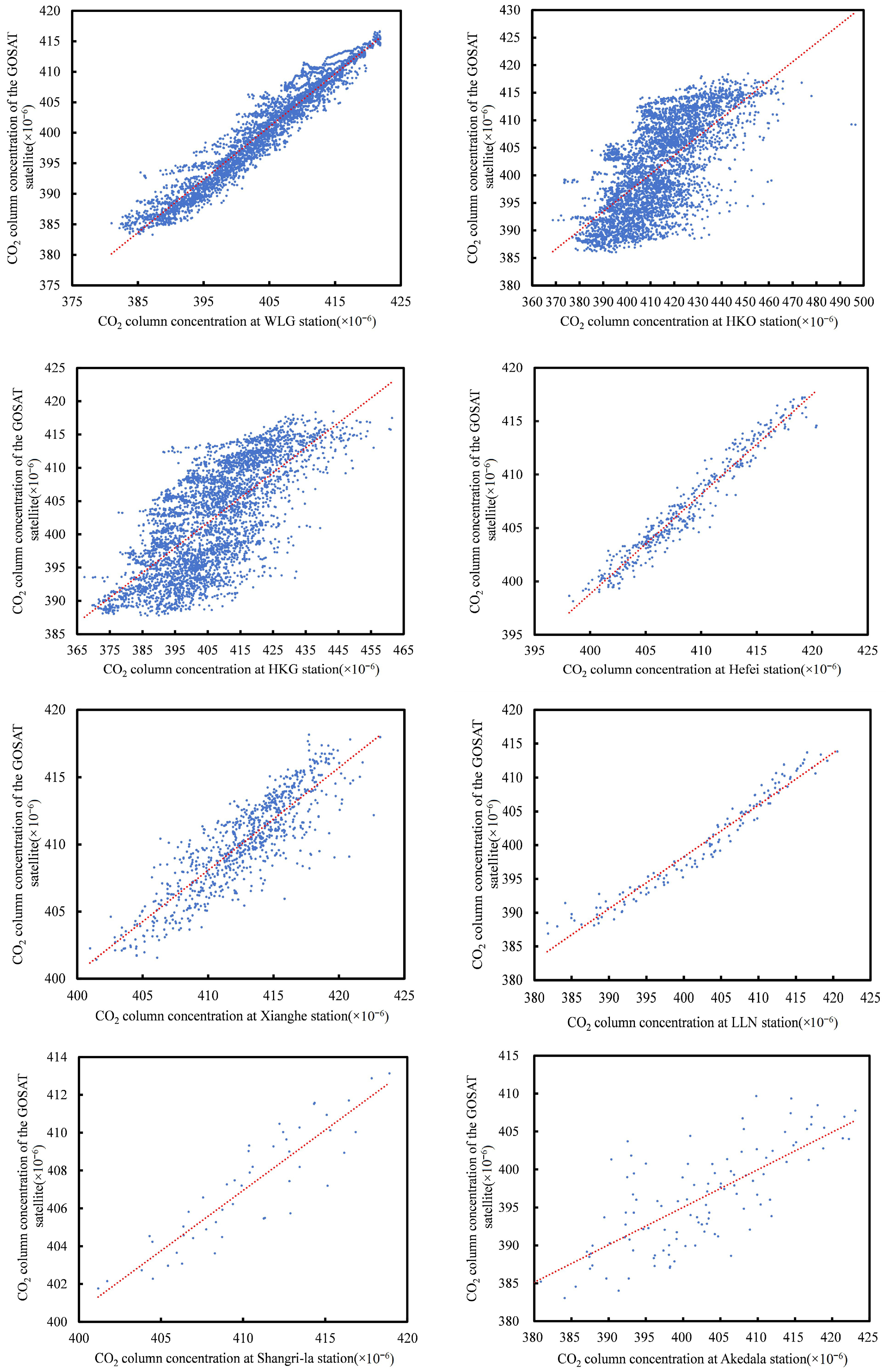
3. Accuracy Validation of CO₂ Observation Data

Given the disparate temporal resolutions of the monthly-resolved GOSAT L3 and 6-hourly L4B products, this study implemented segregated validation protocols to assess the accuracy of these two datasets.

The TCCON operates a global network of ground-based FTIR spectrometers that measure column-averaged CO₂ concentrations via solar absorption spectroscopy [16], achieving a precision of 0.2%. These high-precision ground-based datasets are particularly suitable for validating remote sensing data [36]. To align with the temporal resolution of the GOSAT data products, daily and monthly averages were derived from TCCON’s original 2 min irregular observations. WDCGG provides CO₂ monitoring data for Global Atmosphere Watch (GAW) background stations. Specially, the WLG station in Qinghai, China, a representative continental site in the Eurasian interior, provides critical validation for satellite observations by capturing regional CO₂ characteristics [37]. The WDCGG maintains multidecadal CO₂ records that effectively characterize the long-term trends. These aggregated datasets were subsequently used for validating both the L3 and L4B satellite products.

Validation results for GOSAT L3 CO₂ retrievals against ground-based measurements are presented in

Table 1. Accuracy validations of GOSAT L3 data for eight ground-based sites.

Site	Average Deviation d/(×10−6)	Standard Deviation of Deviation S/(×10−6)	Correlation Coefficient r	Slope k	Intercept b	Sample Size n
Hefei	−0.2054	1.7590	0.9579	0.9774	9.0886	89
Xianghe	−0.6525	1.4082	0.9710	1.1113	−46.8210	58
WLG	−2.4223	3.1415	0.9493	0.9537	16.3080	149
HKO	−11.4394	10.2034	0.8343	0.5031	195.7700	164
HKG	−4.0315	9.3329	0.8494	0.5032	200.5100	142
LLN	0.1338	2.5275	0.9774	0.8794	49.1150	162
XGLL	−1.7951	2.3388	0.8650	0.7643	95.1690	60
AKDL	−3.8595	6.4396	0.7745	0.5531	175.4900	109
Total	−3.0340	4.6439	0.8974	0.7807	86.8287	933

and Figure 1, while those for L4B CO₂ retrievals are presented in

Table 2. Accuracy validations of GOSAT L4B data for eight ground-based sites.

Site	Average Deviation d/(×10−6)	Standard Deviation of Deviation S/(×10−6)	Correlation Coefficient r	Slope k	Intercept b	Sample Size n
Hefei	−1.7380	1.1484	0.9721	0.9329	25.6600	404
Xianghe	−2.5926	1.9074	0.8596	0.9639	94.8870	816
WLG	−4.5172	2.4126	0.9680	0.8671	49.8140	3741
HKO	−11.7944	12.4882	0.6834	0.3400	260.8100	4269
HKG	−4.1292	10.8409	0.7199	0.3748	249.9400	3853
LLN	−2.2902	2.7374	0.9764	0.7684	90.8850	130
XGLL	−3.1290	2.0319	0.8945	0.6387	145.0800	48
AKDL	−5.8024	6.7609	0.7571	0.4950	197.0000	112
Total	−5.4126	5.2557	0.8370	0.6232	157.0884	13421

and Figure 2. The L3 dataset exhibits a robust correlation coefficient of 0.90, accompanied by a mean bias of −3.03 and standard deviation of 4.64. For L4B data, a strong correlation coefficient of 0.84 is observed, with a mean bias of −5.41 and standard deviation of 5.26. The highest correlation coefficient at the LLN site is attributed to the satellite’s orbit path passing directly over the observation station, while the relatively low correlation coefficient at the HKO site occurs because the satellite scanning trajectory is distant from the observational station. These metrics confirm high consistency between satellite and ground-based observations, demonstrating the reliability of GOSAT L3 and L4B data for atmospheric CO₂ monitoring and spatiotemporal analyses.

Notably, excellent agreement between GOSAT retrievals and ground-based CO₂ measurements was observed at Lulin station, with correlation coefficients reaching 0.98 for L3 products and 0.98 for L4B products. The L3 dataset showed lower mean bias and bias standard deviation compared to L4B, likely attributable to its smaller sample. The presence of few outliers in L4B may further contribute to its reduced accuracy. Nevertheless, both datasets exhibited sufficient precision to meet the analytical requirements of this study.

4. Spatiotemporal Distribution of CO₂ Concentrations

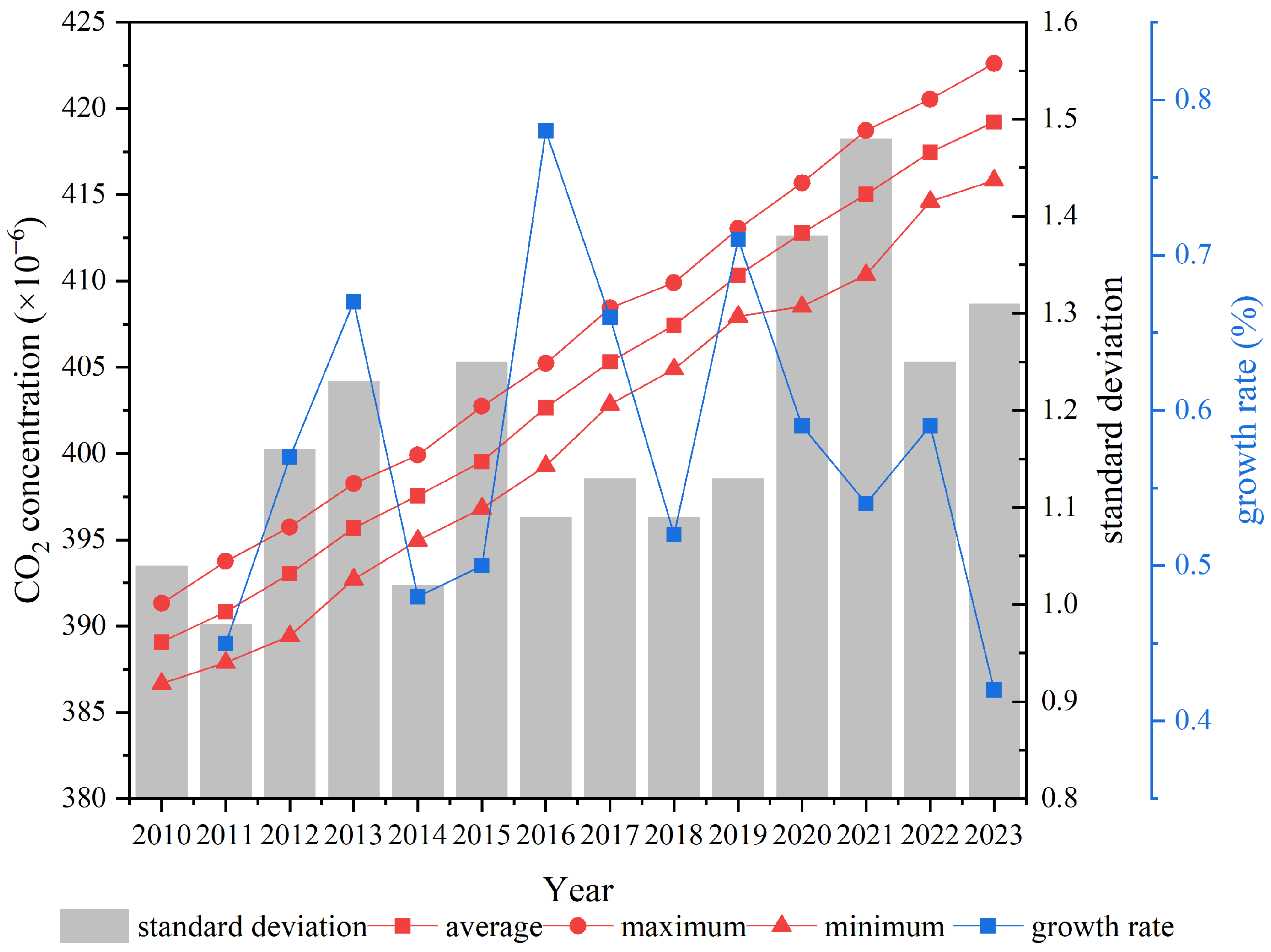
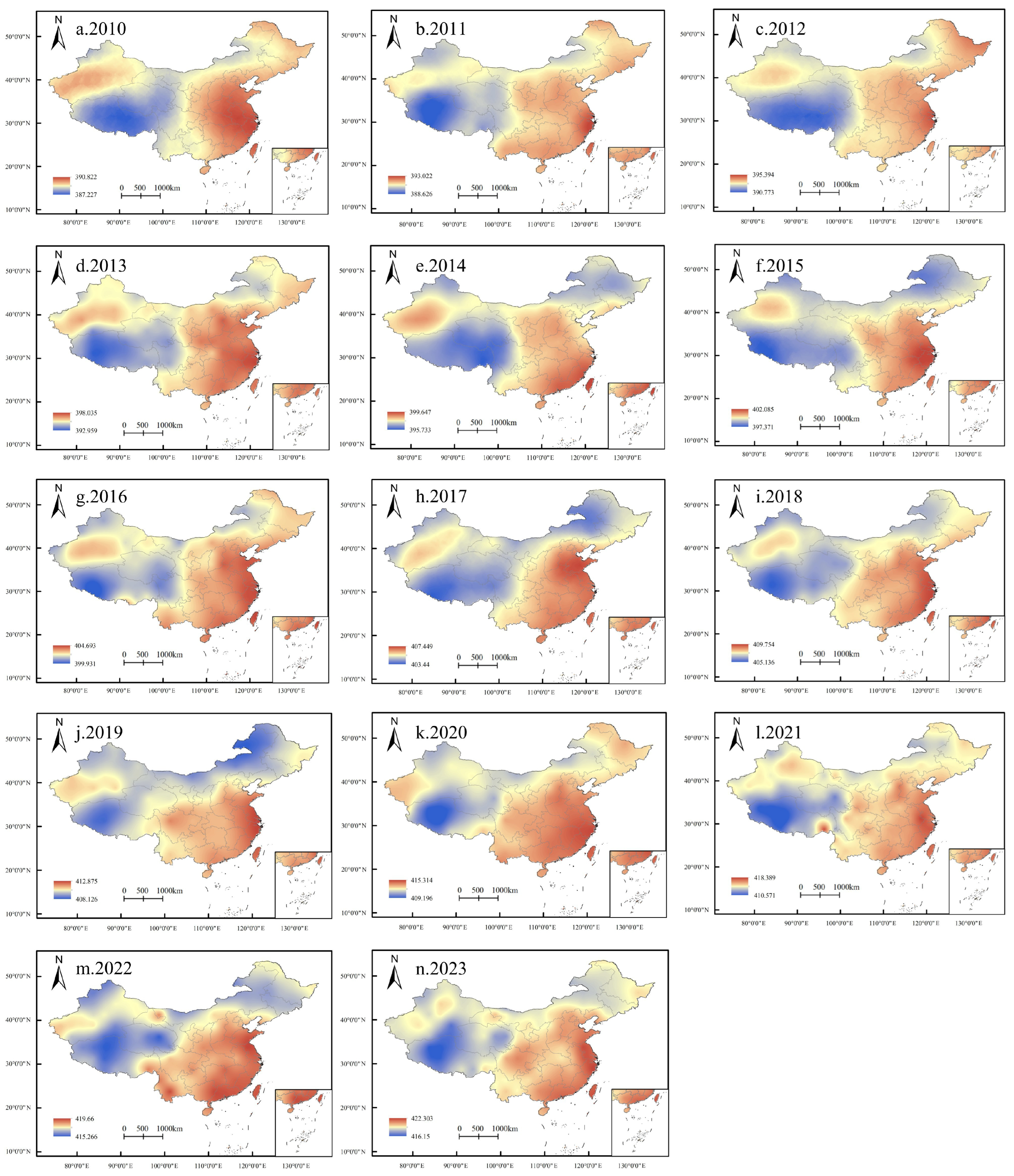
4.1. Annual Changes

As shown in Figure 3, the annual average CO₂ column concentration in China from 2010 to 2023 has shown a gradual upward trend, with both the annual maximum and minimum averages increasing accordingly. The annual average CO₂ column concentration exhibited a near-linear increasing trend, with relatively modest interannual fluctuations. It rose from 389.08 × 10⁻⁶ in 2010 to 419.22 × 10⁻⁶ in 2023, reflecting a total increase of 7.75% over the 13-year period. The maximum CO₂ concentration increased by approximately 8%, while the minimum concentration showed slightly lower growth of approximately 7.54%. The average annual growth rate of the CO₂ column concentration is 0.58%/year. The highest growth rate was observed between 2015 and 2016, reaching 0.78%/year. This increase can be attributed to the rapid industrialization and urbanization during that period. The growing demand for energy, driven by infrastructure construction, industrial production, and heavy reliance on coal-based fossil energy consumption, led to a significant increase in CO₂ emissions [38,39]. By contrast, the 2022–2023 growth rate was the smallest (0.42%), probably attributed to the effects of series of carbon emission control policies and technological advancements. Additionally, the gradually improved carbon trading market and increased adoption of clean energy sources also played a crucial role in curbing CO₂ emission growth [40].

Overall, during the period from 2010 to 2023, the average CO₂ column concentration in China was approximately 404 × 10⁻⁶, with average maximum and minimum values of 406.8 × 10⁻⁶ and 400.92 × 10⁻⁶, respectively. The standard deviation was 1.18, indicating a relatively high degree of dispersion in the distribution of high and low CO₂ concentrations. This variation can be attributed to differences in economic growth rates, industrial structure adjustments, and the content and implementation intensity of energy policies across different provinces [41]. Notably, the increasing trend in the standard deviation of the CO₂ column concentration suggests a gradual expansion of high-value regions. This is attributed to the fact that atmospheric circulation transports CO₂ from regions with high emissions to other areas, leading to a gradual increase in CO₂ concentrations in areas with originally lower CO₂ emissions. Additionally, CO₂ has a relatively long residence time in the atmosphere, and the stable weather conditions further exacerbate the accumulation of CO₂ [1,42].

As illustrated in Figure 4, the spatial distribution of national CO₂ concentrations from 2010 to 2023 maintained a stable “east-high, west-low” pattern, with the locations of high/low-concentration regions remaining largely unchanged. Specifically, high-value areas were predominantly concentrated in eastern and central China, such as the North China Plain, the Yangtze River Delta, and the Pearl River Delta, likely due to rapid economic development, continuous increase in energy consumption, and dominance of fossil fuels. In addition, industrially developed and energy intensive regions such as Shandong Province and the Yangtze River Delta exhibited significantly higher CO₂ emissions and concentrations compared to other regions [43]. Low-value areas were principally located in western and northern China, including the Tibetan Plateau and parts of Inner Mongolia. These areas, characterized by sparse populations, limited industrial activities, and low energy consumption, exhibit correspondingly low CO₂ emissions [44,45]. It is worth noting that the boundary between high and low CO₂ concentrations exhibited a pronounced westward expansion trend, indicating that the scope of high-value areas is gradually increasing. This is in line with the inter-annual variation in standard deviation presented in Figure 3. Historically, northeastern China, a coal-rich heavy industry base with long heating periods due to cold weather and high energy consumption, has witnessed relatively high CO₂ emissions [13,46]. However, the region has been promoting industrial restructuring and energy transition initiatives in recent years [47]. The slowdown in industrial development, combined with significant population outflows and reduced human activities, has led to a decrease in CO₂ emissions [48]. Consequently, CO₂ concentrations in this area have declined, stabilizing at relatively lower levels compared to other regions in recent years.

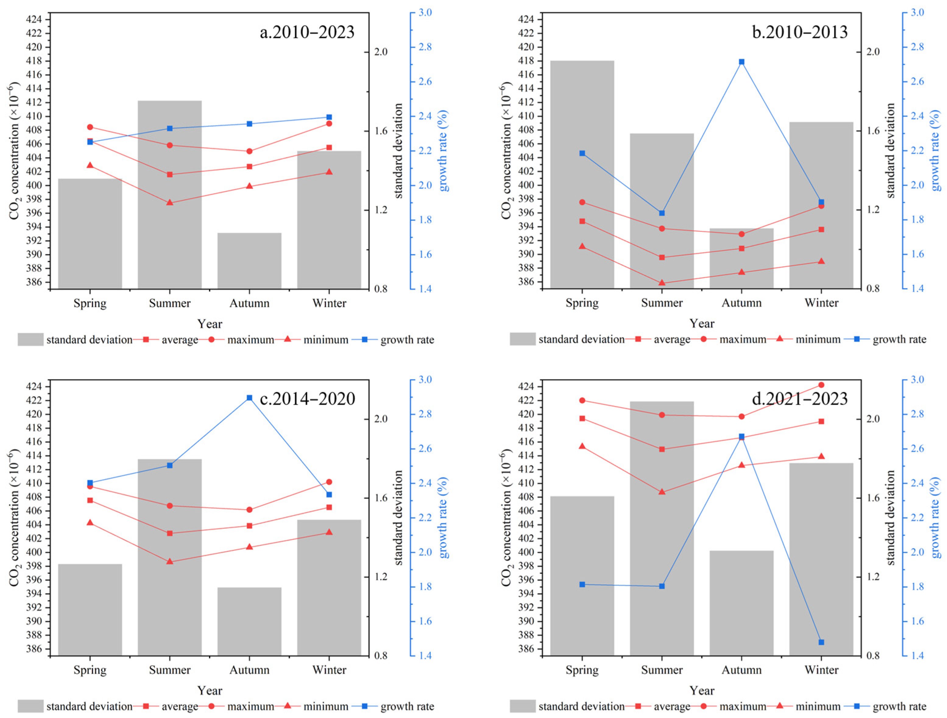
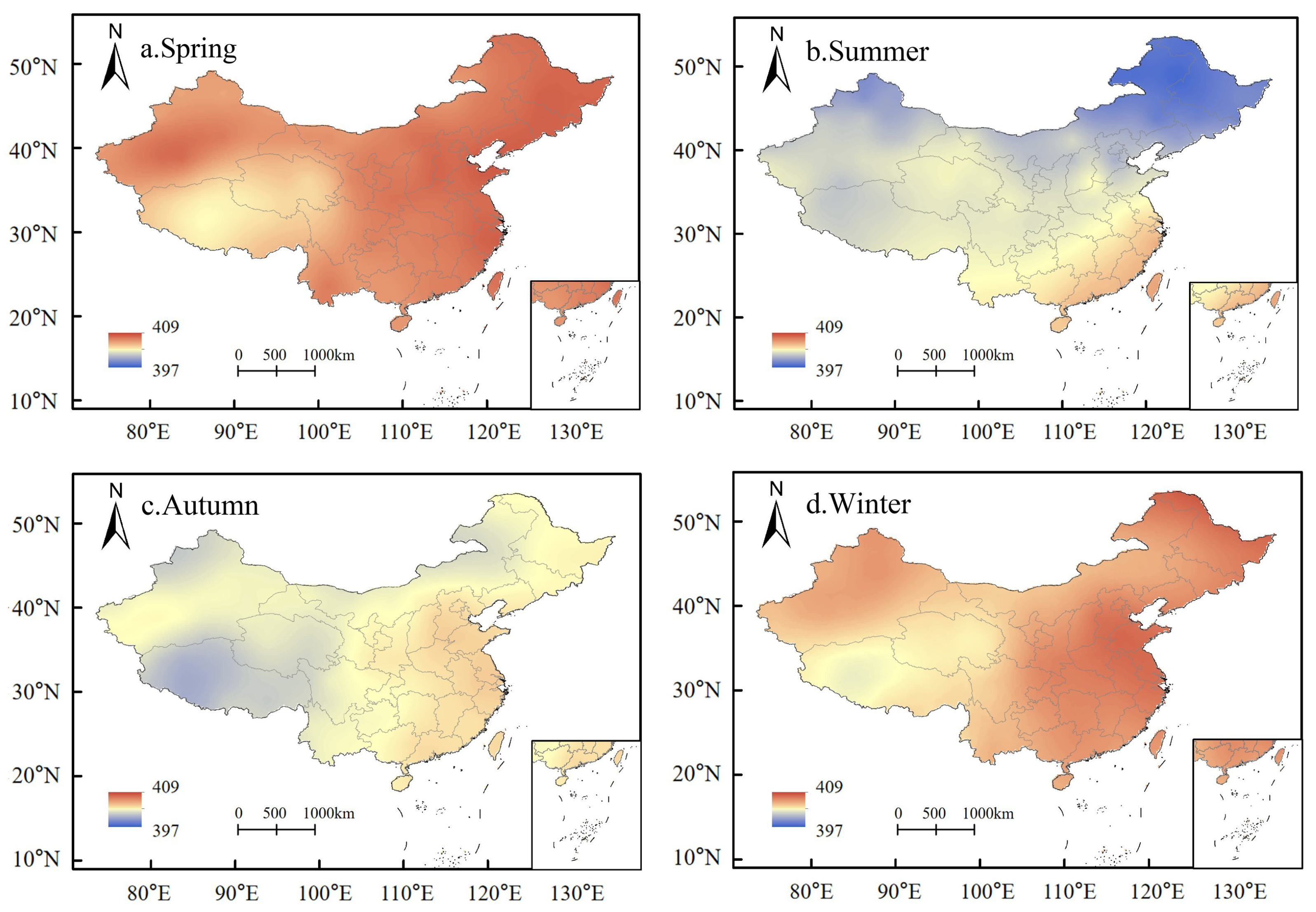
4.2. Multi-Year Seasonal Variation

As illustrated in Figure 5a, during 2010–2023, the atmospheric CO₂ column concentration over China exhibited a seasonal peak in spring (406.39 × 10⁻⁶), closely followed by winter values. In contrast, the lowest concentrations occurred in summer (401.59 × 10⁻⁶). The standard deviation of the CO₂ column concentration was greater in summer and smaller in autumn. This suggests stronger regional heterogeneity in summer CO₂ distribution, potentially driven by varying biospheric activities and meteorological conditions, while more uniform atmospheric mixing exists in autumn.

To investigate policy impacts on CO₂ concentrations, this study divided 2010–2023 into three distinct phases: 2010–2013, 2014–2020 (implementation of the Air Pollution Prevention and Control Action Plan in 2013), and 2021–2023 (introduction of the dual carbon goals in 2020) [3,49]. It was found that during 2010–2013, CO₂ column concentrations exhibited peak standard deviations in spring. This intensified regional concentration disparity likely stems from multiple factors, including low central heating coverage, prevalent decentralized coal combustion, accelerated industrialization, and widespread pre-planting straw burning activities concentrated in the North China Plain and northeast regions, the occurrence of which is significantly lower in southern areas [50,51,52]. The temporal overlap between heating season termination in northern China and industrial resumption in southern regions, as well as the relatively lax straw burning regulations during 2010–2013, leading to the compounded anthropogenic carbon emissions, thereby resulting in the higher spatiotemporal heterogeneity. Following the implementation of the Air Pollution Prevention and Control Action Plan, the phasing out of coal-fired boilers in certain regions reduced decentralized coal usage and agricultural burning regulations were improved, thereby modulating the carbon emissions in the subsequent periods [53,54,55,56]. In the comparison between these three periods, CO₂ concentrations in China showed the highest growth rates in autumn, particularly during the 2014–2020 phase, resulting from combined effects of reduced photosynthesis in vegetations, accelerated plant decomposition, enhanced soil microbial activity during autumn droughts, and increased coal use during the transitions of heating season [57,58,59]. The lowest growth rates occurred in summer during 2010–2013 due to industrial production controls under the 11th Five-Year Plan’s emission policies, while in 2014–2023 they shifted to winter, reflecting the successful carbon reduction through coal-to-gas transitions and renewable energy adoption [56,60].

As shown in Figure 6a, during spring, regions with elevated CO₂ column concentrations are primarily distributed across northeastern China, eastern coastal areas, and western Xinjiang, exhibiting values from 407 × 10⁻⁶ to 409 × 10⁻⁶. In contrast, the Qinghai–Tibet Plateau demonstrates relatively lower concentrations, ranging from 403 × 10⁻⁶ to 405 × 10⁻⁶. Spatially, these concentrations display a distinct north–south gradient, with higher values prevalent in northern regions. This pattern is partially attributed to warmer spring temperatures, which enhance soil microbial activity and trigger the onset of plant growth [61]. Meanwhile, microbial decomposition of organic matter accumulated during the previous winter releases substantial CO₂. Notably, in northeast China, a key industrial and agricultural zone, spring tillage practices and associated soil disturbance further amplify CO₂ emissions. Coastal zones characterized by dense populations, clustered urban infrastructure, and intensive industrial and transportation activities exhibit significantly higher CO₂ emissions, primarily driven by extensive fossil fuel consumption. The compounding effects of energy-intensive economic growth further amplify these emissions [62]. In western Xinjiang, desertification processes and prevailing arid climatic conditions severely constrain vegetation growth, significantly reducing the region’s CO₂ sequestration capacity [63]. Moreover, this region would experience supplementary CO₂ emissions from localized anthropogenic sources, particularly industrial operations and hydrocarbon extraction activities. The Qinghai–Tibet Plateau maintains near-net CO₂ neutrality due to its unique high-altitude climate: low temperatures and limited biomass production restrict CO₂ uptake through photosynthesis and emissions from biological respiration. This natural balance is further reinforced by the low population density and negligible industrial development, resulting in minimal anthropogenic CO₂ inputs to the regional budget.

Figure 6b reveals pronounced spatial heterogeneity in summer atmospheric CO₂ column concentrations across China, with high values (403–405 × 10⁻⁶) in anthropogenically dominated southeastern coastal regions and low values (397–399 × 10⁻⁶) in northeast China. This pattern exhibits a clear latitudinal gradient, with CO₂ concentrations increasing from north to south. In the economically developed southeastern coastal region, summertime CO₂ emissions arise from the peak electricity demand and intensive fossil fuel combustion for industrial and residential use. Moreover, high population density and concentrated transportation networks in this region further amplify CO₂ emissions. In contrast, northeastern China demonstrates robust CO₂ sequestration, facilitated by vigorous summer vegetation growth and extensive forest coverage that enhance photosynthetic uptake [63,64,65]. Additionally, cooler summer temperatures in northeast China substantially reduce air-conditioning demand, leading to lower electricity consumption compared to southern regions.

Figure 6c illustrates distinct autumn spatial patterns in CO₂ column concentrations, with high values (403–405 × 10⁻⁶) across north and east China and low values (398–400 × 10⁻⁶) over the Qinghai–Tibet Plateau, forming a pronounced east-to-west decreasing gradient. North China, a key agricultural and industrial base, emits CO₂ from mechanized farming, crop residue burning, and energy-intensive manufacturing, transportation, and residential energy consumption [62]. In contrast, the Qinghai–Tibet Plateau’s low temperatures, sparse vegetation cover, and minimal anthropogenic activity limit both carbon uptake [65] and emissions, maintaining low CO₂ concentrations.

Wintertime concentrations in Figure 6d show marked heterogeneity: northeast and east China have high values (407 × 10⁻⁶–409 × 10⁻⁶), while the Qinghai–Tibet Plateau remains low (401 × 10⁻⁶–403 × 10⁻⁶) due to its geographical environment. Northeast China’s cold winter drives intensive fossil fuel combustion for heating [66]. Continued industrial activity further contributes to CO₂ emissions. East China’s robust economy and dense population maintain high emissions from industry, transportation, and residential heating [62,67]. Conversely, the Qinghai–Tibet Plateau’s sparse human settlements and negligible industrial activity result in minimal winter CO₂ emissions.

In summary, the atmospheric CO₂ column concentration is highest in spring and lowest in summer in China. High-concentration regions persist in north and east China during spring, autumn, and winter, with spatial patterns influenced by climate, vegetation dynamics, seasonal practices, and anthropogenic activities. Notably, spring/autumn highs correlate closely with agricultural and industrial activities, while summer/winter distributions are more strongly driven by climatic conditions and regional industrial intensity.

5. Vertical Distribution of CO₂

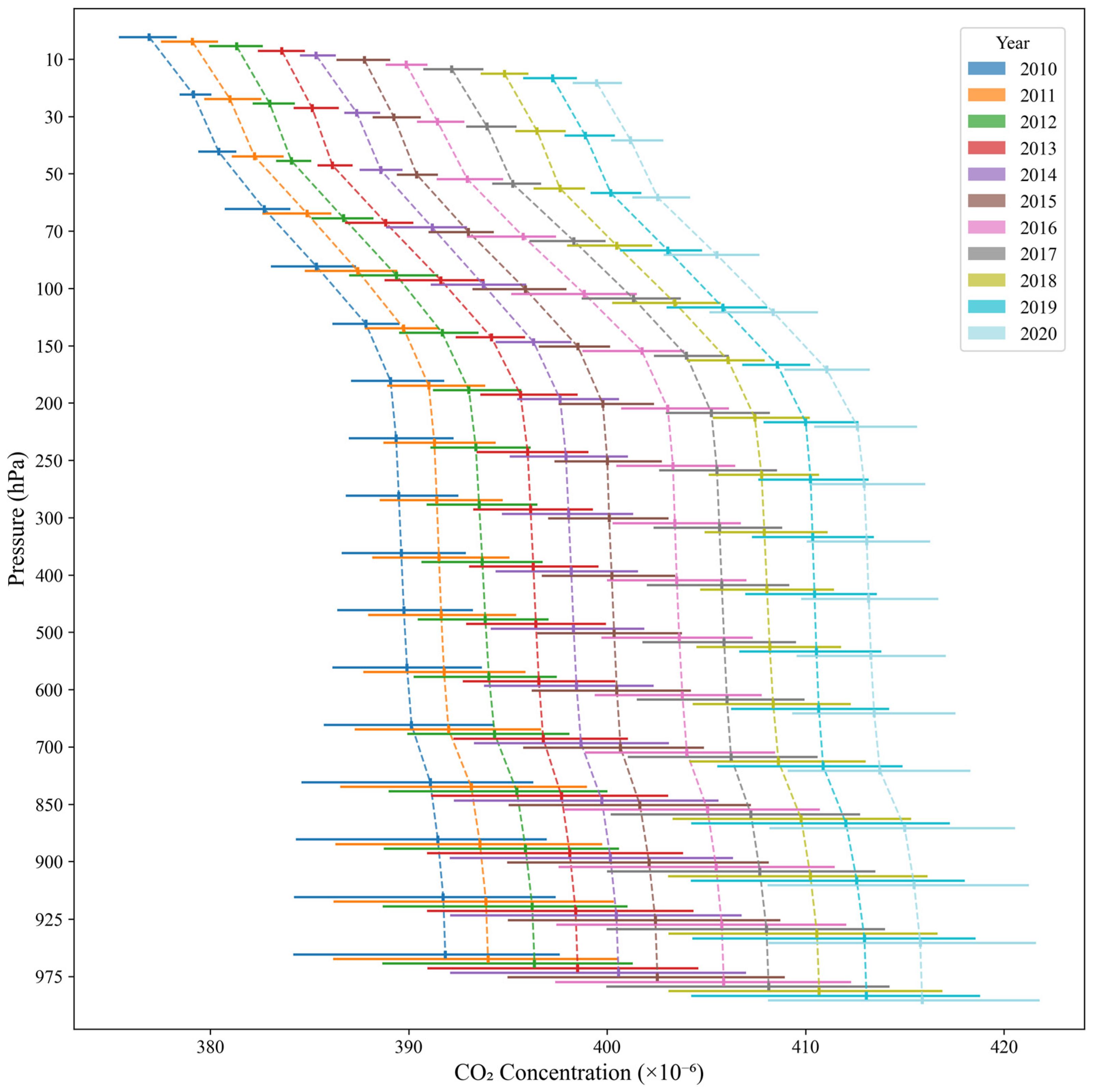
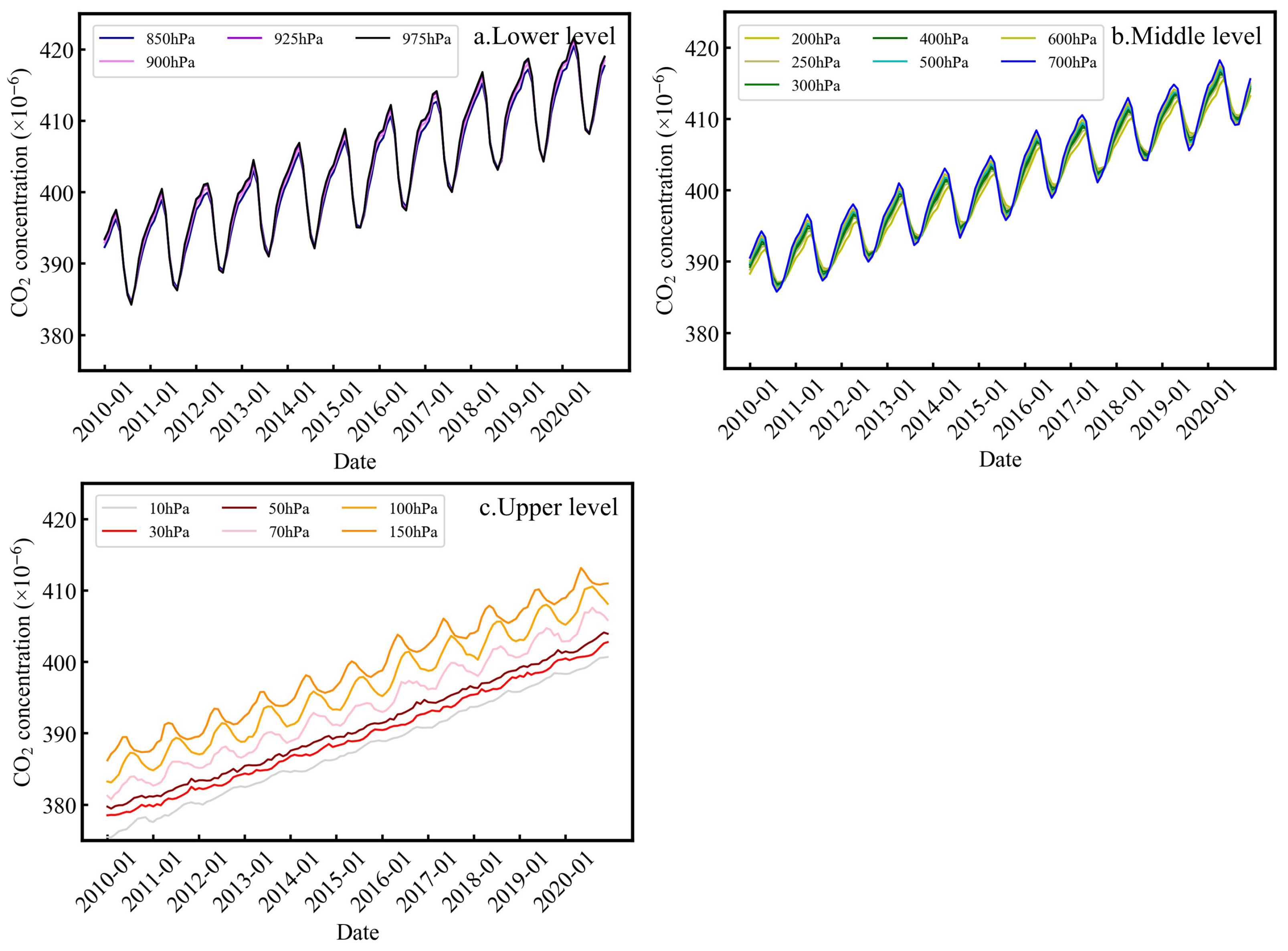
5.1. Multi-Year Vertical Distribution

Figure 7 shows that CO₂ concentrations decreased with decreasing atmospheric pressure (increasing altitude) from 2010 to 2020. The rate of decrease and range differed across altitude levels. Specifically, CO₂ concentrations near the surface (~1000 hPa) remained consistently high (390 × 10⁻⁶–420 × 10⁻⁶), which is attributed to surface-level anthropogenic activities, including industrial production, transportation, and residential emissions [67]. In the 200–1000 hPa layer, CO₂ concentrations show a significant upward trend, reflecting rising energy consumption from economic growth that elevates near-surface CO₂ emissions, with the mid-troposphere showing a cumulative response to these sources [68,69]. Above 200 hPa, CO₂ concentrations decline most rapidly with increasing altitude, and interannual concentration differences diminish, likely due to the reduced surface influence and dominance of global-scale atmospheric circulation and mixing processes [70].

CO₂ concentrations exhibit systematic vertical variations, accompanied by uncertainty ranges that initially diminish, then expand with altitude. Below 30 hPa, uncertainties progressively decrease with increasing altitude, whereas they increase substantially above 30 hPa to 10 hPa. Specifically, the difference between the upper and lower limits of the uncertainty range is 13.90 × 10⁻⁶ at lower levels (975 hPa), but decreases to 2.44 × 10⁻⁶ at higher levels (10 hPa).

Figure 8 demonstrates temporal CO₂ concentration variations at 17 pressure levels over China. CO₂ remains well mixed throughout the troposphere [71], with minimal concentration differences between surface (975 hPa) and middle tropospheric (200 hPa) levels, consistent with findings of Machida [72]. Notably, CO₂ at and below 70 hPa (lower stratosphere and below) exhibits distinct monthly periodicity, whereas no significant cyclical patterns are observed above 50 hPa. This discrepancy is driven by strong vertical mixing in the lower stratosphere, which facilitates rapid upward transport of surface emissions [70]. Consequently, CO₂ concentrations within this altitude range are directly influenced by pronounced seasonal near-surface emissions. In contrast, the 50 hPa level resides in the mid-stratosphere, where stable atmospheric stratification and dominant horizontal transport mechanisms minimize convective impacts.

5.2. Seasonal Vertical Distribution

Figure 9 shows that CO₂ concentrations decrease with decreasing atmospheric pressure (increasing altitude) during spring, autumn, and winter, driven by surface emissions from anthropogenic activities and energy use. During summer, CO₂ concentrations increase with increasing altitude (decreasing pressure) below 200 hPa, but decrease with increasing altitude above this level. This pattern likely stems from two concurrent processes: vigorous vegetation photosynthesis reduces near-surface CO₂ levels, while active vertical convection transports residual surface CO₂ upward, creating the maximum concentration in the mid-troposphere [73,74].

Seasonal variations differ by altitude: CO₂ concentrations in the 1000–200 hPa layer peak in spring, coinciding with delayed vegetation recovery and wintertime CO₂ accumulation from stable atmospheric conditions and enhanced soil microbial respiration [49,50]. Notably, the lowest CO₂ concentrations occur in summer within the 1000–600 hPa layer, but shift to autumn above 600–200 hPa, potentially linked to combined effects from atmospheric circulation and vegetation phenology [75]. Above 200 hPa, seasonal variations in CO₂ profiles are minimal as surface influences diminish, with concentrations governed primarily by large-scale circulation.

Vertical gradients of CO₂ concentration are steeper in the 1000–700 hPa layer than 700–200 hPa, reflecting stronger surface-convection interactions (e.g., low-altitude precipitation scavenging pollutants) enhancing vertical mixing at lower levels.

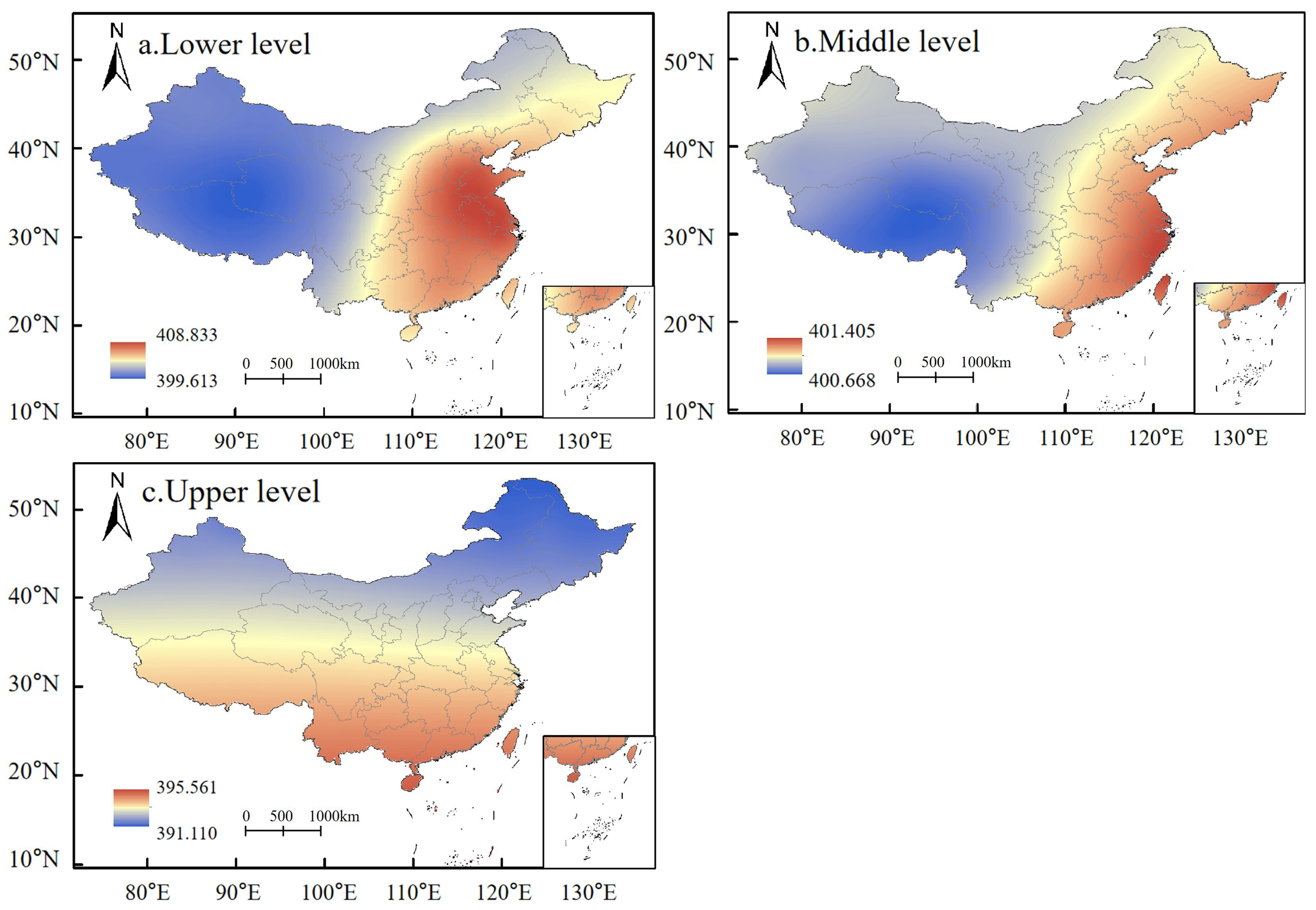
5.3. Spatial Characteristics at Different Levels

As shown in Figure 10, lower-tropospheric CO₂ hotspots are predominantly located in eastern China, which is the most populous and economically dynamic region. Intensive industrial operations, high-density transportation networks, and concentrated residential energy consumption drive substantial fossil fuel combustion, yielding substantial CO₂ emissions [76]. Furthermore, the expansive urban agglomerations generate pronounced urban heat island effects, stabilizing the atmospheric boundary layer through thermal inversions [77]. These conditions suppress vertical mixing, trapping emissions near the surface and fostering persistent CO₂ accumulation. In contrast, the Xinjiang, Tibet, and Qinghai plateau junction, characterized by harsh natural environments, sparse populations, underdeveloped economies, and minimal industrial activity, exhibits notably low CO₂ concentrations due to suppressed anthropogenic emissions.

A mid-tropospheric CO₂ hotspot is centered over the Yangtze River Delta, a major economic hub with dense industrial clusters, high population density, and elevated emissions. Here, atmospheric circulation patterns and local meteorological conditions synergistically transport long-lived CO₂ from the lower troposphere to mid-altitude layers in this mid-latitude region [78]. The Tibetan Plateau exhibits distinctively low CO₂ concentrations due to its unique plateau meteorology: strong vertical mixing driven by thermal pumping effects efficiently disperses surface emissions [79], and the peripheral updrafts of the South Asian High suppress the accumulation of pollutants, resulting in the low CO₂ concentration in this area.

High CO₂ concentration in the upper atmospheric layers is observed over southern China, predominantly resulting from variations in weather conditions. For example, the subtropical westerly jet stream exhibits strong vertical wind shear, inducing turbulent mixing, and enhances vertical transport processes of lower-tropospheric CO₂ to higher layers [80]. In contrast, northeastern China demonstrates depressed CO₂ levels due to the enhanced horizontal advective transport and efficient dilution of localized CO₂ concentrations, which is induced by the frequent incursions of dry and cold polar air masses coupled with the Northeast China Cold Vortex.

The distinct discrepancy in the spatial pattern of CO₂ levels between the mid-lower and upper troposphere should be noted. This is because CO₂ concentration patterns in the middle and lower atmospheric layers exhibit pronounced dual regulation from anthropogenic and natural sources. On one hand, near-surface industrial and transportation emissions directly elevate CO₂ concentrations, particularly evident in eastern coastal China with its intensive industrial production and high energy consumption [62], while enhanced air–sea CO₂ exchange amplifies marine carbon influences there. On the other hand, CO₂ concentrations in the upper atmosphere are predominantly regulated by large-scale circulation dynamics. Compared to the middle and lower atmospheric layers, the upper layer exhibits lower sensitivity to proximal emission sources and terrestrial–aquatic carbon exchange systems, including human-induced discharges and biospheric fluxes.

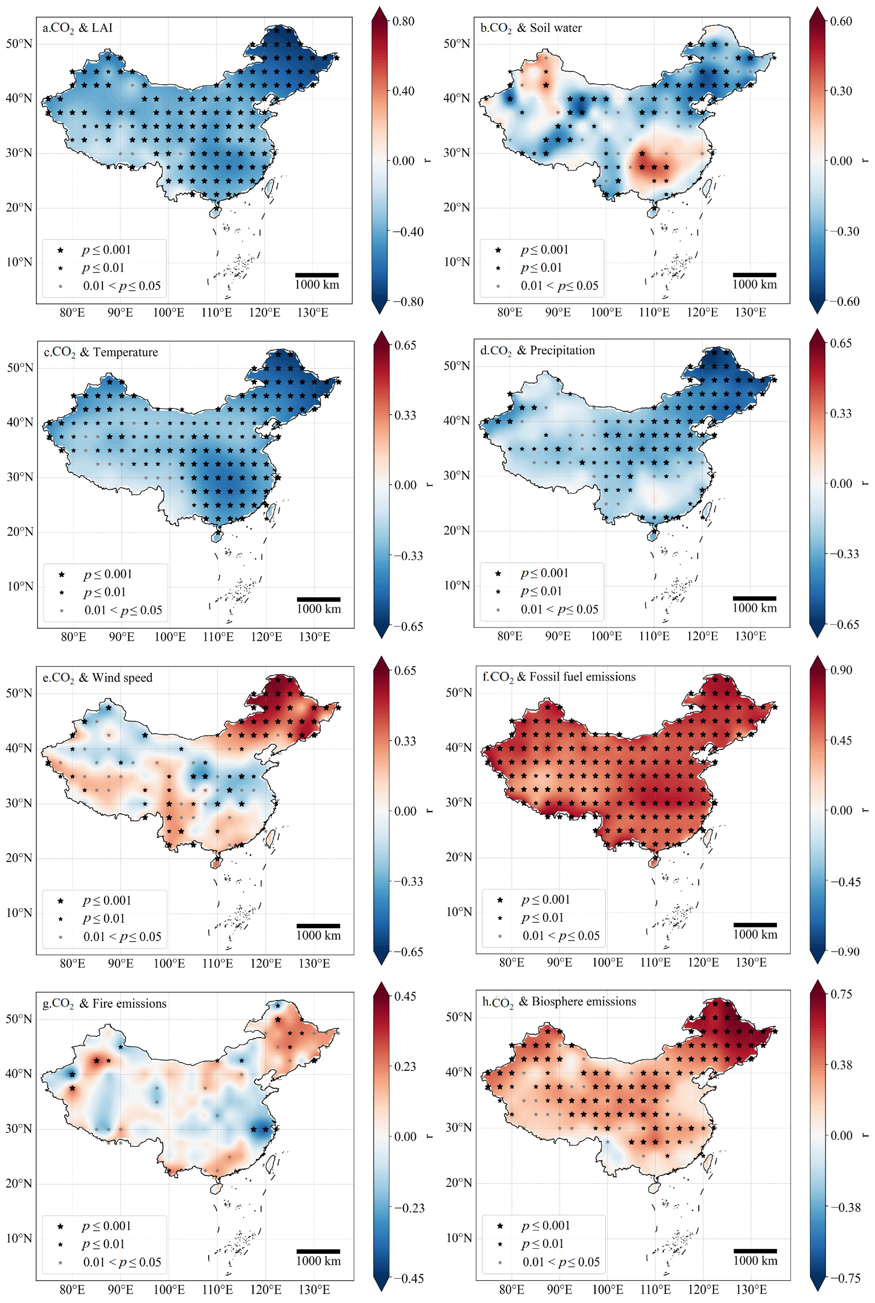
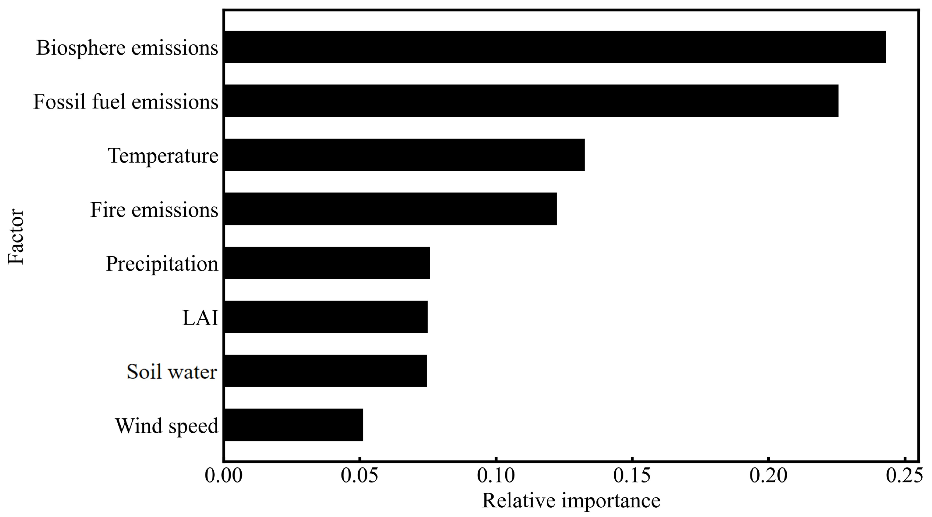
6. Factors Influencing CO₂ Concentration

To quantify the effects of different factors on atmospheric CO₂ concentration, we conducted correlation analyses based on multi-source datasets, including atmospheric CO₂ concentration at the 975 hPa isobaric level from the GOSAT L4B satellite product, meteorological variables from the ERA5 reanalysis, and emission estimates of fossil fuel, fire, and biosphere from CarbonTracker.

As illustrated in Figure 11, spatial heterogeneity exists in the correlations between atmospheric CO₂ concentration and its influencing factors (e.g., meteorological conditions, vegetation indices, and anthropogenic emissions). Specifically, a significant negative correlation (p < 0.05) was observed between LAI and atmospheric CO₂ concentration across China. The strongest negative correlation (r = −0.6 to −0.8) occurred in northeast China, where temperate mixed forests and grasslands dominate. These ecosystems exhibit high LAI and substantial biomass accumulation, leading to enhanced photosynthetic CO₂ uptake during the growing season, likely resulting in the pronounced negative correlation in this region [81].

Soil water content (SWC) demonstrates pronounced regional heterogeneity in its correlation with CO₂ concentrations. Significant positive correlations (p < 0.05) were detected in parts of central China and northern Xinjiang, while negative correlations predominated in other areas. The highest correlations (r = −0.4 to −0.6) occurred in the Bohai Sea coastal region, where saline–alkali soils prevail. High soil salinity significantly suppresses soil microbial activity, thereby reducing CO₂ emissions and contributing to the observed negative relationship [82].

Additionally, there is a significant negative correlation between temperature and atmospheric CO₂ concentration (p < 0.05). Spatial heterogeneity also exists, i.e., the strongest negative correlation (r = −0.4 to −0.6) occurs in northeast China, which is predominantly covered by temperate mixed forest ecosystems [83]. Climate-driven warming in this region promotes vegetation growth, enhancing photosynthetic CO₂ uptake and driving the observed negative correlation [84].

Precipitation also correlates significantly negatively to CO₂ concentrations (p < 0.05), with peak values in northeastern China (r = −0.45 to −0.65). Here, black soil and marsh soil combined with excessive precipitation can lead to long-term waterlogging and poor aeration, inhibiting root respiration and microbial activity and thereby greatly reducing soil CO₂ emissions [85]. Additionally, abundant vegetation in this region experiences disrupted metabolism under excessive rainfall, with wetland ecosystems and unique climatic conditions further amplifying precipitation’s negative effect on CO₂ concentrations.

Wind speed demonstrates significant spatial heterogeneity in its correlation with atmospheric CO₂ concentrations. A predominant positive correlation exists nationwide, while negative correlations emerge in eastern and central China. Northeastern China exhibits the strongest positive signals (r = 0.4–0.6).

Fossil fuel emissions are significantly positively correlated with the atmospheric CO₂ concentration across China. The correlations are relatively high in the northeast region and the middle and lower reaches of the Yangtze River (r > 0.6, p < 0.05). This is because of northeastern China’s large-scale heavy industry and the Yangtze River region’s intensive transportation, resulting in large amounts of CO₂ emissions.

Fire emissions in northeast China show a positive correlation with CO₂ concentrations (r ≈ 0.2), whereas the Yangtze River Estuary exhibits a distinct negative correlation (r = −0.2 to −0.4). This divergence is likely driven by the coastal region’ s monsoon-driven atmospheric circulation, and the East Asian monsoon rapidly transports the fire-emitted CO₂ from the Yangtze River estuary to the East China Sea and the Pacific Ocean, reducing the local concentration [86].

Biosphere emissions show significant positive correlations with CO₂ concentrations nationwide, except for weak negative signals in parts of Yunnan (r ≈ −0.1). The strongest correlations (r = 0.5 to 0.7) occur in northeast China, where forest–agricultural ecosystems dominate. During autumn, a large amount of CO₂ is released through leaf litter decomposition and soil microbial activity. Furthermore, fertilizer application intensity and agricultural machinery energy inputs both contribute to the carbon emissions in farmland ecosystems across northeast China [87].

This study employed a random forest model to quantify the relative importance of factors influencing CO₂ concentrations. Firstly, the predictive performance of the random forest model was systematically evaluated through a multi-dimensional index. The results show that R² of the model on the test set reaches 0.313, while that on the training set is 0.430. Error analysis reveals that the RMSE and MAE of the test set are 8.015 × 10⁻⁶ and 6.812 × 10⁻⁶, respectively. The average deviation between predicted and measured values remains within 6.8–8.0 × 10⁻⁶, demonstrating the model’s robust predictive accuracy.

Variable importance analysis (Figure 12) reveals the key driving factors affecting CO₂ concentrations. Biosphere emissions (24%) and fossil fuel emissions (23%) emerge as dominant factors, consistent with the strong positive correlations (r > 0.6) observed in industrialized regions such as northeastern China and the Yangtze River Basin. As secondary contributors, temperature (13%) and fire emissions (12%) reflect the impact of climate change and extreme events. In contrast, environmental factors such as precipitation, LAI, soil water, and wind speed (all <10%) show relatively weak direct contributions, likely due to their predominant indirect effects through temperature regulation and biological emissions.

In conclusion, atmospheric CO₂ concentration dynamics are mainly driven by direct anthropogenic activities and natural emissions, while climate and surface processes exerting relatively minor impacts. These findings emphasize the need to focus on the management of fossil fuel use and biological emissions in carbon reduction policies and to include climate factors such as temperature and fires in long-term monitoring.

7. Discussion

Compared to existing studies, this study extended the temporal coverage of study period and employed a coupled correlation analysis–random forest approach to quantify the relative importance of factors influencing CO₂ variations. The results showed that the temporal characteristics of CO₂ concentrations aligned with the findings provided by Zhu et al., while the importance ranking of influencing factors was consistent with those of Zhu et al. and Cheng et al. to some extent [26,88]. However, Zhu et al. conducted an analysis of relative importance using only aggregated CO₂ emission and concentrations, whereas our study employed source-specific CO₂ emissions (i.e., fossil fuel emissions, fire emissions, and biosphere emissions), thereby providing more detailed information on the impacts of carbon emission on CO₂ variations [26]. Furthermore, previous satellite studies showed limited attention to the vertical spatial distribution patterns of CO₂ concentrations in China. The present study analyzed the vertical distribution of CO₂ across different temporal scales and the spatial distributions of CO₂ at varied vertical layers, as well as investigated the underlying mechanisms governing these distribution characteristics. Additionally, we employed the random forest model to quantify the contribution of various external factors to CO₂ concentration variations and identify the key factors.

Despite undertaking a systematic investigation of the spatiotemporal patterns and factors influencing CO₂ concentrations in China, several limitations still exist in this study. For example, previous studies found that natural carbon fluxes exert significant influences on CO₂ concentrations across China, particularly affecting their spatiotemporal distribution patterns and playing a crucial role in understanding CO₂ concentration variations [89,90]. Additionally, cross-regional transport is found to be another key pathway influencing CO₂ concentrations [91,92]. Currently, the primary approaches used to investigate the impacts of carbon fluxes and cross-regional transport on CO₂ concentrations are numerical model simulations [93,94]. For example, Fang et al. employed the FLEXPART model to analyze the source attribution of CO₂ concentrations in northern China based on ground-based station and satellite observations, demonstrating that the representative regions of carbon sources and sinks exhibit significant seasonal variations [94]. The areas adjacent to the study locations are predominant CO₂ source and sink regions. However, the impacts of natural carbon fluxes and cross-regional transport on CO₂ concentrations are difficult to systematically analyze based on the correlation analysis and random forest model employed in this study, and require perfectly matched data dimensions across all variables. Therefore, future studies should employ model simulations to address the abovementioned knowledge gaps, thereby enabling a comprehensive assessment of the impacts of all potential factors influencing CO₂ variations.

8. Conclusions

Rising CO₂ concentrations pose significant challenges to climate and ecosystems. The spatiotemporal distribution patterns of CO₂ concentration and the factors influencing CO₂ concentration were investigated in this study. The results showed the following.

(1)

From 2010 to 2023, CO₂ column concentrations showed a consistent annual increase over China, rising from 389.08 × 10⁻⁶ to 419.22 × 10⁻⁶. The spatial distribution exhibited a clear “east-high and west-low” pattern, with higher concentrations in industrialized eastern regions like north China, the Yangtze River Delta, and the Pearl River Delta and lower concentrations in western regions, including the Tibetan Plateau and Inner Mongolia.

(2)

CO₂ concentrations reach their peak in spring (406.39 × 10⁻⁶) and their lowest value in summer (401.59 × 10⁻⁶). Northern and eastern China maintain relatively high concentrations year-round, while the Qinghai–Tibet Plateau consistently exhibits lower levels. During summer, the highest concentrations concentrate in the southeastern coastal regions, and the lowest concentrations occur in northeastern China.

(3)

Regarding the vertical profile of CO₂, concentrations generally decrease with increasing altitude. However, during summer, strong photosynthetic activity reduces surface concentrations, leading to an increase in CO₂ levels with increasing height below 200 hPa. Spatial distribution patterns of CO₂ differ across vertical layers: higher concentration at the lower layer is located in eastern China, while southern China exhibits elevated CO₂ levels at higher altitudes. Throughout the atmospheric column, the Qinghai–Tibet Plateau consistently maintains lower CO₂ concentrations.

(4)

CO₂ emissions are the dominant drivers of CO₂ variation, with biosphere emissions contributing 24% and fossil fuel emissions contributing 23%. Temperature (13%) and fire emissions (12%) served as secondary climatic controls, while vegetation indices, precipitation, and wind speed played more modest modulating roles (each <10%). These driving factors exhibited significant spatial heterogeneity in their impacts across different regions of China.

The results further suggested that enhancing carbon emission reductions from major emission sources, i.e., fossil fuel combustion and biosphere emissions under specific meteorological conditions (e.g., low temperature and low precipitation), in key regions such as economically developed eastern coastal areas and industrialized zones is crucial for achieving the dual carbon goals in a comprehensive manner. This study provides valuable insights for developing targeted mitigation strategies to facilitate sustained carbon reduction.

References

1. Calvin, K.; Dasgupta, D.; Krinner, G.; Mukherji, A.; Thorne, P.W.; Trisos, C.; Romero, J.; Aldunce, P.; Barrett, K.; Blanco, G.; et al. Climate Change 2023: Synthesis Report. Contribution of Working Groups I, II and III to the Sixth Assessment Report of the Intergovernmental Panel on Climate Change; Core Writing Team, Lee, H., Romero, J., Eds.; IPCC: Geneva, Switzerland, 2023. [Google Scholar]
2. Ge, Y.; Xiao, Z. Analysis on the Spatial and Temporal Characteristics of CO2 Concentration in China Based on GOSAT Satellite. Environ. Monit. China 2022, 38, 96–108. [Google Scholar]
3. Zhong, P. The New Situation of Global Climate Change and the New Potential of Climate Friendly Technologies. China Sustain. Trib. 2020, 10, 40–42. [Google Scholar]
4. Lei, L.; Guan, X.; Zeng, Z.; Zhang, B.; Ru, F.; Bu, R. A Comparison of Atmospheric CO2 Concentration GOSAT-Based Observations and Model Simulations. Sci. China Earth Sci. 2014, 57, 1393–1402. [Google Scholar] [CrossRef]
5. Gurney, K.R.; Law, R.M.; Denning, A.S.; Rayner, P.J.; Baker, D.; Bousquet, P.; Bruhwiler, L.; Chen, Y.-H.; Ciais, P.; Fan, S.; et al. Towards Robust Regional Estimates of CO2 Sources and Sinks Using Atmospheric Transport Models. Nature 2002, 415, 626–630. [Google Scholar] [CrossRef] [PubMed]
6. Hungershoefer, K.; Breon, F.-M.; Peylin, P.; Chevallier, F.; Rayner, P.; Klonecki, A.; Houweling, S.; Marshall, J. Evaluation of Various Observing Systems for the Global Monitoring of CO2 Surface Fluxes. Atmos. Chem. Phys. 2010, 10, 10503–10520. [Google Scholar] [CrossRef]
7. Rayner, P.J.; O’Brien, D.M. Correction to “The Utility of Remotely Sensed CO2 Concentration Data in Surface Source Inversions”. Geophys. Res. Lett. 2001, 28, 2429. [Google Scholar] [CrossRef]
8. Houweling, S.; Breon, F.-M.; Aben, I.; Rödenbeck, C.; Gloor, M.; Heimann, M.; Ciais, P. Atmospheric Chemistry and Physics Inverse Modeling of CO2 Sources and Sinks Using Satellite Data: A Synthetic Inter-Comparison of Measurement Techniques and Their Performance as a Function of Space and Time. Atmos. Chem. Phys. 2004, 4, 523–538. [Google Scholar] [CrossRef]
9. Miller, C.E.; Crisp, D.; DeCola, P.L.; Olsen, S.C.; Randerson, J.T.; Michalak, A.M.; Alkhaled, A.; Rayner, P.; Jacob, D.J.; Suntharalingam, P.; et al. Precision Requirements for Space-Based XCO2 Data. J. Geophys. Res. Atmos. 2007, 112, D10314. [Google Scholar] [CrossRef]
10. Chevallier, F. Impact of Correlated Observation Errors on Inverted CO2 Surface Fluxes from OCO Measurements. Geophys. Res. Lett. 2007, 34, L24804. [Google Scholar] [CrossRef]
11. Chen, L.; Zhang, Y.; Zou, M.; Xu, Q.; Li, L.; Li, X.; Tao, J. Overview of Atmospheric CO2 Remote Sensing from Space. Natl. Remote Sens. Bull. 2015, 19, 1–11. [Google Scholar] [CrossRef]
12. Li, J.; Jia, K.; Wei, X.; Xia, M.; Chen, Z.; Yao, Y.; Zhang, X.; Jiang, H.; Yuan, B.; Tao, G.; et al. High-Spatiotemporal Resolution Mapping of Spatiotemporally Continuous Atmospheric CO2 Concentrations over the Global Continent. Int. J. Appl. Earth Obs. Geoinf. 2022, 108, 102743. [Google Scholar] [CrossRef]
13. Yang, D.; Yang, X.; Wu, X. Spatio-Temporal Evolution Characteristics of Carbon Emissions from Energy Consumption and Its Driving Mechanism in Northeast China. Acta Sci. Circumstantiae 2018, 38, 4554–4564. [Google Scholar]
14. Yin, S.; Wang, X.; Tani, H.; Zhang, X.; Zhong, G.; Sun, Z.; Chittenden, A.R. Analyzing Temporo-Spatial Changes and the Distribution of the CO2 Concentration in Australia from 2009 to 2016 by Greenhouse Gas Monitoring Satellites. Atmos. Environ. 2018, 192, 1–12. [Google Scholar] [CrossRef]
15. Imasu, R.; Tanabe, Y. Diurnal and Seasonal Variations of Carbon Dioxide (CO2) Concentration in Urban, Suburban, and Rural Areas around Tokyo. Atmosphere 2018, 9, 367. [Google Scholar] [CrossRef]
16. Deng, A.; Guo, H.; Hu, J.; Jiang, C.; Liu, P.; Jing, H. Temporal and Distribution Characteristic of CO2 Concentration over China Based on GOSAT Satellite Data. Natl. Remote Sens. Bull. 2020, 24, 319–325. [Google Scholar] [CrossRef]
17. Lv, Z.; Shi, Y.; Zang, S.; Sun, L. Spatial and Temporal Variations of Atmospheric CO2 Concentration in China and Its Influencing Factors. Atmosphere 2020, 11, 231. [Google Scholar] [CrossRef]
18. Lv, Y.; Ma, Y.; Li, H.; Ding, Y.; Meng, Q.; Guo, J. Analysis of Spatiotemporal Patterns of Atmospheric CO2 Concentration in the Yellow River Basin over the Past Decade Based on Time-Series Remote Sensing Data. Environ. Sci. Pollut. Res. Int. 2023, 30, 115745–115757. [Google Scholar] [CrossRef] [PubMed]
19. Gao, Y.; Liu, S.; Hu, N.; Wang, S.; Deng, L.; Yu, Z.; Zhang, Z.; Li, X. Direct Observation on the Temporal and Spatial Patterns of the CO2 Concentration in the Atmospheric of Nanjing Urban Canyon in Summe. Environ. Sci. 2015, 36, 2367–2373. [Google Scholar]
20. Liu, X.; Cheng, X.; Hu, F. Gradient Characteristics of CO2 Concentration and Flux in Beijing Urban Area Part I: Concentration and Virtual Temperature. Chin. J. Geophys. 2015, 58, 1502–1512. (In Chinese) [Google Scholar]
21. Sun, P.; Yuan, K.; Hu, S.; Huang, J. Statistical Analysis of Lower-Troposphere CO2 Vertical Distribution Measured by Raman Lidar in Hefei Western Suburb. Guangxue Xuebao/Acta Opt. Sin. 2016, 36, 1101001. [Google Scholar] [CrossRef]
22. Xiao, J.; Xie, B.; Zhou, K.; Li, J.; Xie, J.; Liang, C. Contributions of Climate Change, Vegetation Growth, and Elevated Atmospheric CO2 Concentration to Variation in Water Use Efficiency in Subtropical China. Remote Sens. 2022, 14, 4296. [Google Scholar] [CrossRef]
23. Chen, X.; He, Q.; Ye, T.; Liang, Y.; Li, Y. Decoding Spatiotemporal Dynamics in Atmospheric CO2 in Chinese Cities: Insights from Satellite Remote Sensing and Geographically and Temporally Weighted Regression Analysis. Sci. Total Environ. 2024, 908, 167917. [Google Scholar] [CrossRef] [PubMed]
24. Yurak, V.V.; Fedorov, S.A. Review of Natural and Anthropogenic Emissions of Carbon Dioxide into the Earth’s Atmosphere. Int. J. Environ. Sci. Technol. 2025, 22, 2719–2736. [Google Scholar] [CrossRef]
25. Mustafa, F.; Bu, L.; Wang, Q.; Ali, M.A.; Bilal, M.; Shahzaman, M.; Qiu, Z. Multi-Year Comparison of CO2 Concentration from NOAA Carbon Tracker Reanalysis Model with Data from GOSAT and OCO-2 over Asia. Remote Sens. 2020, 12, 2498. [Google Scholar] [CrossRef]
26. Zhu, W.; Zhang, H.; Zhang, X.; Guo, H.; Liu, Y. Evaluating the Spatiotemporal Variations in Atmospheric CO2 Concentrations in China and Identifying Factors Contributing to Its Increase. Atmos. Pollut. Res. 2025, 16, 102458. [Google Scholar] [CrossRef]
27. Wu, D.; Yue, Y.; Jing, J.; Liang, M.; Sun, W.; Han, G.; Lou, M. Background Characteristics and Influence Analysis of Greenhouse Gases at Jinsha Atmospheric Background Station in China. Atmosphere 2023, 14, 1541. [Google Scholar] [CrossRef]
28. Song, X.; Duan, X.; Peng, X.; Yin, Y.; Li, X. Study on Screening and Concentration Characteristics of Atmospheric CO2 Data from Shangri La Regional Atmospheric Background Station. J. Agric. Catastrophology 2025, 15, 170–172. [Google Scholar]
29. Cohen, H.W. P Values: Use and Misuse in Medical Literature. Am. J. Hypertens. 2011, 24, 18–23. [Google Scholar] [CrossRef] [PubMed]
30. Brereton, R.G. The Use and Misuse of p Values and Related Concepts. Chemom. Intell. Lab. Syst. 2019, 195, 103884. [Google Scholar] [CrossRef]
31. Huang, K.; Xiao, Q.; Meng, X.; Geng, G.; Wang, Y.; Lyapustin, A.; Gu, D.; Liu, Y. Predicting Monthly High-Resolution PM2.5 Concentrations with Random Forest Model in the North China Plain. Environ. Pollut. 2018, 242, 675–683. [Google Scholar] [CrossRef] [PubMed]
32. Zheng, L.; Lin, R.; Wang, X.; Chen, W. The Development and Application of Machine Learning in Atmospheric Environment Studies. Remote Sens. 2021, 13, 4839. [Google Scholar] [CrossRef]
33. Meng, F.; Tan, Y.; Bu, Y. Target Aggregation Regression Based on Random Forests. Procedia Comput. Sci. 2022, 199, 517–523. [Google Scholar] [CrossRef]
34. Tsigaridis, K.; Daskalakis, N.; Kanakidou, M.; Adams, P.J.; Artaxo, P.; Bahadur, R.; Balkanski, Y.; Bauer, S.E.; Bellouin, N.; Benedetti, A.; et al. The AeroCom Evaluation and Intercomparison of Organic Aerosol in Global Models. Atmos. Chem. Phys. 2014, 14, 10845–10895. [Google Scholar] [CrossRef]
35. Chicco, D.; Warrens, M.J.; Jurman, G. The Coefficient of Determination R-Squared Is More Informative than SMAPE, MAE, MAPE, MSE and RMSE in Regression Analysis Evaluation. PeerJ Comput. Sci. 2021, 7, e623. [Google Scholar] [CrossRef] [PubMed]
36. Wunch, D.; Toon, G.C.; Blavier, J.F.L.; Washenfelder, R.A.; Notholt, J.; Connor, B.J.; Griffith, D.W.T.; Sherlock, V.; Wennberg, P.O. The Total Carbon Column Observing Network. Philos. Trans. R. Soc. A Math. Phys. Eng. Sci. 2011, 369, 2087–2112. [Google Scholar] [CrossRef] [PubMed]
37. Zhou, L.; Zhou, X.; Zhang, X.; Wen, Y.; Yan, P. Progress in the Study of Background Greenhouse Gases at Waliguan Observatory. Acta Meteorol. Sin. 2007, 65, 458–468. [Google Scholar]
38. Lin, B.; Liu, X. China’s Carbon Dioxide Emissions under the Urbanization Process: Influence Factors and Abatement Policies. Econ. Res. J. 2010, 8, 66–78. [Google Scholar]
39. Zhao, H.; You, A.; Yang, W.; Wang, D. China Regional Economic Development Report (2015–2016); Social Sciences Academic Press: Beijing, China, 2016; ISBN 9787509790878. [Google Scholar]
40. Wang, K.; Lv, C. Achievements and Prospect of China’s National Carbon Market Construction (2024). J. Beijing Inst. Technol. Soc. Sci. Ed. 2024, 26, 16–27. [Google Scholar]
41. Zhang, Z.; Yu, Y.; Wang, D.; Kharrazi, A.; Ren, H.; Zhou, W.; Ma, T. Socio-Economic Drivers of Rising CO2 Emissions at the Sectoral and Sub-Regional Levels in the Yangtze River Economic Belt. J. Environ. Manag. 2021, 290, 112617. [Google Scholar] [CrossRef] [PubMed]
42. Pérez, I.A.; Sánchez, M.L.; García, M.Á.; Pardo, N.; Fernández-Duque, B. The Influence of Meteorological Variables on CO2 and CH4 Trends Recorded at a Semi-Natural Station. J. Environ. Manag. 2018, 209, 37–45. [Google Scholar] [CrossRef] [PubMed]
43. Ge, F.; Li, J.; Zhang, Y.; Ye, S.; Han, P. Impacts of Energy Structure on Carbon Emissions in China, 1997–2019. Int. J. Environ. Res. Public Health 2022, 19, 5850. [Google Scholar] [CrossRef] [PubMed]
44. Nie, H.; Mo, J. Spatiotemporal Dynamics of Carbon Dioxide Emissions Distribution in China: A Study Utilizing Input-Output Theor. Soc. Sci. Front. 2024, 7, 80–92. [Google Scholar]
45. Hao, R.; Wei, W.; Liu, C.; Xie, B.; Du, H. Spatialization and Spatio-Temporal Dynamics of Energy Consumption Carbon Emissions in China. Environ. Sci. 2022, 43, 5305–5314. [Google Scholar]
46. Wei, Y.; Xie, Z. Investigation of the Historical Context of the Development and Revitalization of the Industrial Economy in Northeast China after the Founding of the People’s Republic of China. Liaoning Econ. 2024, 11, 64–66. [Google Scholar]
47. Li, S. The Impact of Industrial Structure Upgrading on My Country’s Carbon Emission Reduction from the Perspective of High-Quality Development. Sustain. Dev. 2021, 11, 149–159. [Google Scholar] [CrossRef]
48. Mu, X.; Fan, Z.; Tong, X. On the Impact and Countermeasures of Population Loss on Economy in Northeast China. J. Hainan Norm. Univ. 2025, 1, 113–120. [Google Scholar]
49. Yang, S.; Wang, F.; Liu, N. Assessment of the Air Pollution Prevention and Control Action Plan in China: A Difference-in-Difference Analysis. China Popul. Resour. Environ. 2020, 30, 110–117. [Google Scholar]
50. Xu, B.; Fan, M.; Chen, L.; Jiang, T.; Tao, J.; Cheng, L.; Ji, X.; Wu, W. Analysis of Temporal and Spatial Characteristics and Influonling Factors of Crop Residue Burning in Major Agricultural Areas from 2013 to 2017. Yaogan Xuebao/J. Remote Sens. 2020, 24, 1221–1232. [Google Scholar] [CrossRef]
51. Xie, H.; Du, L.; Liu, S.; Chen, L.; Gao, S.; Liu, S.; Pan, H.; Tong, X. Dynamic Monitoring of Agricultural Fires in China from 2010 to 2014 Using MODIS and GlobeLand30 Data. ISPRS Int. J. Geoinf. 2016, 5, 172. [Google Scholar] [CrossRef]
52. Zhuang, Y.; Li, R.; Yang, H.; Chen, D.; Chen, Z.; Gao, B.; He, B. Understanding Temporal and Spatial Distribution of Crop Residue Burning in China from 2003 to 2017 Using MODIS Data. Remote Sens. 2018, 10, 390. [Google Scholar] [CrossRef]
53. Ren, H. Implementing Clean Energy Action to Improve Air Quality in China. Environ. Impact Assess. 2014, 4, 28–30. [Google Scholar]
54. Zhou, M.; Liu, H.; Peng, L.; Qin, Y.; Chen, D.; Zhang, L.; Mauzerall, D.L. Environmental Benefits and Household Costs of Clean Heating Options in Northern China. Nat. Sustain. 2022, 5, 329–338. [Google Scholar] [CrossRef]
55. Meng, W.; Zhong, Q.; Chen, Y.; Shen, H.; Yun, X.; Smith, K.R.; Li, B.; Liu, J.; Wang, X.; Ma, J.; et al. Energy and Air Pollution Benefits of Household Fuel Policies in Northern China. Proc. Natl. Acad. Sci. USA 2019, 116, 16773–16780. [Google Scholar] [CrossRef] [PubMed]
56. Fang, P.; Zhang, W.; Song, L.L.; Xu, Z.; Wu, Z.M.; Lei, Z.Y.; Hu, T.J.; Li, M.Y.; Chen, L.; Li, J.S. Benefit Assessment of Mercury Emission Reductions under the Cleaner Heating Policy for the Rural Households in Northern China. Zhongguo Huanjing Kexue/China Environ. Sci. 2023, 43, 981–992. [Google Scholar]
57. Wang, J.; Xu, Y.; Ding, F.; Gao, X.; Li, S.; Sun, L.; An, T.; Pei, J.; Li, M.; Wang, Y.; et al. Process of Plant Residue Transforming into Soil Organic Matter and Mechanism of Its Stabilization: A Review. Acta Pedol. Sin. 2019, 56, 528–540. [Google Scholar] [CrossRef]
58. Li, X.; Zhang, Z.; Dang, Z.; Wang, C. Effects of Drought on Soil Microorganism and Its Relationship with Carbon Dynamics. J. Shanxi Agric. Sci. 2018, 46, 402–406. [Google Scholar]
59. Luo, Y. Response of Soil Microorganism to Elevated Atmospheric CO2 Concentration. Ecol. Environ. 2003, 12, 357–360. [Google Scholar]
60. Dong, W. Analysis of the Situation of Pollution Reduction in China in the Late Stage of the Eleventh Five Year Plan. Environ. Pollut. Control 2008, 11, 99–100+107. [Google Scholar]
61. Parazoo, N.C.; Koven, C.D.; Lawrence, D.M.; Romanovsky, V.; Miller, C.E. Detecting the Permafrost Carbon Feedback: Talik Formation and Increased Cold-Season Respiration as Precursors to Sink-to-Source Transitions 2017. Cryosphere 2017, 12, 123–144. [Google Scholar] [CrossRef]
62. Zhang, Y.; Niu, J.; Xin, B.; Wang, M.; Guo, J. Temporal and Spatial Differences and Influencing Factors of Urban Carbon Emissions in Bohai Rim Region. J. Hebei Acad. Sci. 2024, 6, 15–24. [Google Scholar]
63. Xie, X. Study on the interactions of air pollution, vegetation and carbon dioxide in China. Master’s Thesis, Nanjing University, Nanjing, China, 2020. [Google Scholar]
64. Chao, B.; Bao, G.; Yuan, Z.; Wen, D.; Tong, S.; Guo, E.; Huang, X. Sensitivity of the Peaking Time of the Growing Season and Peak EVI to Climate at the Middle and High Latitudes of the Northern Hemisphere during 2001–2020. Prog. Geogr. 2023, 42, 1809–1824. [Google Scholar] [CrossRef]
65. Randerson, J.T.; Thompson, M.V.; Conway, T.J.; Fung, I.Y.; Field, C.B. The Contribution of Terrestrial Sources and Sinks to Trends in the Seasonal Cycle of Atmospheric Carbon Dioxide. Glob. Biogeochem. Cycles 1997, 11, 535–560. [Google Scholar] [CrossRef]
66. Kuttippurath, J.; Peter, R.; Singh, A.; Raj, S. The Increasing Atmospheric CO2 over India: Comparison to Global Trends. iScience 2022, 25, 104863. [Google Scholar] [CrossRef] [PubMed]
67. Liu, D.; Lei, L.; Guo, L.; Zeng, Z.C. A Cluster of CO2 Change Characteristics with GOSAT Observations for Viewing the Spatial Pattern of CO2 Emission and Absorption. Atmosphere 2015, 6, 1695–1713. [Google Scholar] [CrossRef]
68. Wang, S.; Zhou, C.; Li, G.; Feng, K. CO2, Economic Growth, and Energy Consumption in China’s Provinces: Investigating the Spatiotemporal and Econometric Characteristics of China’s CO2 Emissions. Ecol. Indic. 2016, 69, 184–195. [Google Scholar] [CrossRef]
69. Zhao, M.; Lv, L.; Zhang, B.; Luo, H. Dynamic Relationship Among Energy Consumption, Economic Growth and Carbon Emissions in China. Res. Environ. Sci. 2021, 34, 1509–1522. [Google Scholar]
70. Li, Y.; Deng, J.; Mu, C.; Xing, Z.; Du, K. Vertical Distribution of CO2 in the Atmospheric Boundary Layer: Characteristics and Impact of Meteorological Variables. Atmos. Environ. 2014, 91, 110–117. [Google Scholar] [CrossRef]
71. Friedlingstein, P.; O’Sullivan, M.; Jones, M.W.; Andrew, R.M.; Bakker, D.C.E.; Hauck, J.; Landschützer, P.; Le Quéré, C.; Luijkx, I.T.; Peters, G.P.; et al. Global Carbon Budget 2023. Earth Syst. Sci. Data 2023, 15, 5301–5369. [Google Scholar] [CrossRef]
72. Machida, T.; Kita, K.; Kondo, Y.; Blake, D.; Kawakami, S.; Inoue, G.; Ogawa, T. Vertical and Meridional Distributions of the Atmospheric CO2 Mixing Ratio between Northern Midlatitudes and Southern Subtropics. J. Geophys. Res. Atmos. 2002, 107, BIB 5-1–BIB 5-9. [Google Scholar] [CrossRef]
73. He, Z.; Lei, L.; Zeng, Z.-C.; Sheng, M.; Welp, L.R. Evidence of Carbon Uptake Associated with Vegetation Greening Trends in Eastern China. Remote Sens. 2020, 12, 718. [Google Scholar] [CrossRef]
74. Esteki, K.; Prakash, N.; Li, Y.; Mu, C.; Du, K. Seasonal Variation of CO2 Vertical Distribution in the Atmospheric Boundary Layer and Impact of Meteorological Parameters. Int. J. Environ. Res. 2017, 11, 707–721. [Google Scholar] [CrossRef]
75. Zhang, M.; Zhang, X.; Liu, R. Study on the Accuracy of Satellite Hyperspectral Atmospheric CO2 Remote Sensing Retrieval and Ground-Based Verification. Adv. Clim. Change Res. 2014, 10, 427–432. [Google Scholar]
76. Wang, Z.; Cui, C.; Peng, S. How Do Urbanization and Consumption Patterns Affect Carbon Emissions in China? A Decomposition Analysis. J. Clean. Prod. 2019, 211, 1201–1208. [Google Scholar] [CrossRef]
77. Sun, M.; Zhang, J.; Qu, Y. The Impact of Urban Heat Island Effect on Urban and Rural Pollutant Transport. Rural. Econ. Sci.-Technol. 2021, 22, 28–30. [Google Scholar]
78. Diallo, M.; Legras, B.; Ray, E.; Engel, A.; Añel, J.A. Global Distribution of CO2 in the Upper Troposphere and Stratosphere. Atmos. Chem. Phys. 2017, 17, 3861–3878. [Google Scholar] [CrossRef]
79. Zhuo, G.; Xu, X.; Chen, L. Dynamical Effect of Boundary Layer Characteristics of Tibetan Plateau on General Circulation. J. Appl. Meteorol. Sci. 2002, 13, 163–169. [Google Scholar]
80. Long, Q.; Jin, R.; Xiao, T.; Yang, N.; Liu, S. Analysis of the Characteristics of the East Asian Subtropical Westerly Jet under Different Scales in Summer. J. Trop. Meterology 2017, 6, 1000–1008. [Google Scholar]
81. Wang, J.; Feng, L.; Palmer, P.I.; Liu, Y.; Fang, S.; Bösch, H.; O’Dell, C.W.; Tang, X.; Yang, D.; Liu, L.; et al. Large Chinese Land Carbon Sink Estimated from Atmospheric Carbon Dioxide Data. Nature 2020, 586, 720–723. [Google Scholar] [CrossRef] [PubMed]
82. Mavi, M.S.; Marschner, P.; Chittleborough, D.J.; Cox, J.W.; Sanderman, J. Salinity and Sodicity Affect Soil Respiration and Dissolved Organic Matter Dynamics Differentially in Soils Varying in Texture. Soil Biol. Biochem. 2012, 45, 8–13. [Google Scholar] [CrossRef]
83. Ye, J.; Yuan, Y.; Cai, L.; Wang, X. Research Progress of Phylogeographic Studies of Plant Species in Temperate Coniferous and Broadleaf Mixed Forests in Northeastern China. Biodivers. Sci. 2017, 25, 1339–1349. [Google Scholar] [CrossRef]
84. Fang, Y.; Liu, D.; Duan, Y.; Huang, K.; Wang, W.; Qin, Y.J.; Wang, A.; Wang, C.; Liu, Y.; Tu, Y. Effects of Climate Warming on Carbon Sink of Forest Ecosystems: Mechanisms, Methods, and Progresses. Chin. J. Ecol. 2024, 43, 2551–2565. [Google Scholar]
85. Gao, Z.; Sun, L.; Wang, L.; Li, W.; Song, B.; Zhang, L.; Du, C. Causes, Harms and Control Measures of Waterlogging in Heilongjiang Province. Heilongjiang Agric. Sci. 2019, 11, 142–148. [Google Scholar]
86. Xie, M.; Wang, T.; Gao, D.; Li, S.; Zhuang, B.; Liu, Z. Impact of Anomalous East Asian Winter Monsoon on the Spatial Distribution of Aerosols over East Asia. Clim. Environ. Res. 2021, 26, 438–448. [Google Scholar]
87. Fan, D.; Yang, X.; Wu, X.; Zhou, J.; Ru, Y. Spatial-Temporal Differentiation of Agro-Ecosystem Carbon Emissions in Northeast China and Its Driving Factors. Acta Sci. Circumstantiae 2017, 37, 2797–2804. [Google Scholar]
88. Cheng, Z.; Wang, W. The Relationship Betwee Carbon Dioxide and Biosphere: The Third of the Global Green House Approaching Series. Res. Environ. Sci. 1990, 3, 38–44. [Google Scholar]
89. Chou, W.C.; Gong, G.C.; Hung, C.C.; Wu, Y.H. Carbonate Mineral Saturation States in the East China Sea: Present Conditions and Future Scenarios. Biogeosciences 2013, 10, 6453–6467. [Google Scholar] [CrossRef]
90. Liu, S.; Liang, J.; Jiang, Z.; Li, J.; Wu, Y.; Fang, Y.; Ren, Y.; Zhang, X.; Huang, X.; Macreadie, P.I. Temporal and Spatial Variations of Air-Sea CO2 Fluxes and Their Key Influence Factors in Seagrass Meadows of Hainan Island, South China Sea. Sci. Total Environ. 2024, 910, 168684. [Google Scholar] [CrossRef] [PubMed]
91. Chen, Y.; Wang, S.; He, W. Global Air-Sea CO2 Flux Inversion Based on Multi-Source Data Fusion and Machine Learning. Chaos Solitons Fractals 2025, 192, 115963. [Google Scholar] [CrossRef]
92. Yamuza-Magdaleno, A.; Jiménez-Ramos, R.; Cavijoli-Bosch, J.; Brun, F.G.; Egea, L.G. Ocean Acidification and Global Warming May Favor Blue Carbon Service in a Cymodocea Nodosa Community by Modifying Carbon Metabolism and Dissolved Organic Carbon Fluxes. Mar. Pollut. Bull. 2025, 212, 117501. [Google Scholar] [CrossRef] [PubMed]
93. Peters, W.; Jacobson, A.R.; Sweeney, C.; Andrews, A.E.; Conway, T.J.; Masarie, K.; Miller, J.B.; Bruhwiler, L.M.P.; Pétron, G.; Hirsch, A.I.; et al. An Atmospheric Perspective on North American Carbon Dioxide Exchange: CarbonTracker. Proc. Natl. Acad. Sci. USA 2007, 104, 18925–18930. [Google Scholar] [CrossRef] [PubMed]
94. Feng, T.; Zhou, W.; Wu, S.; Niu, Z.; Cheng, P.; Xiong, X.; Li, G. High-Resolution Simulation of Wintertime Fossil Fuel CO2 in Beijing, China: Characteristics, Sources, and Regional Transport. Atmos. Environ. 2019, 198, 226–235. [Google Scholar] [CrossRef]
Figure 1. Comparison between GOSAT L3 data and ground-based measurements for eight sites.
Remotesensing 17 02542 g001
Figure 2. Comparison between GOSAT L4B data and ground-based measurements for eight sites.
Remotesensing 17 02542 g002
Figure 3. Annual changes in regional CO2 column concentrations across China during 2010–2023.
Remotesensing 17 02542 g003
Figure 4. Spatial distribution of annual average CO2 column concentration in China from 2010 to 2023.
Remotesensing 17 02542 g004
Figure 5. Seasonal variation in CO2 column concentrations during (a) 2010–2023, (b) 2010–2013, (c) 2014–2020, and (d) 2021–2023 in China.
Remotesensing 17 02542 g005
Figure 6. Spatial distribution of average CO2 column concentrations for (a) Spring, (b) Summer, (c) Autumn and (d) Winter over years in China.
Remotesensing 17 02542 g006
Figure 7. Vertical profile of regional CO2 concentration for China.
Remotesensing 17 02542 g007
Figure 8. Temporal variation in CO2 concentration at (a) lower level (850–975 hPa), (b) middle level (200–700 hPa), and (c) upper level (0–150 hPa) in China.
Remotesensing 17 02542 g008
Figure 9. Vertical profile of regional CO2 concentration for China during different seasons.
Remotesensing 17 02542 g009
Figure 10. Spatial distribution of regional CO2 concentration in China: (a) lower level (850–975 hPa), (b) middle level (200–700 hPa), and (c) upper level (0–150 hPa).
Remotesensing 17 02542 g010
Figure 11. Spatial distribution of correlation coefficients between CO2 concentration and (a) LAI, (b) soil water, (c) temperature, (d) precipitation, (e) wind speed, (f) fossil fuel emissions, (g) fire emissions, and (h) biosphere emissions. Note that the size of each data point indicates the reliability of the correlation.
Remotesensing 17 02542 g011
Figure 12. Relative importance of influencing factors.
Remotesensing 17 02542 g012