Deep Learning and Transformer Models for Groundwater Level Prediction in the Marvdasht Plain: Protecting UNESCO Heritage Sites—Persepolis and Naqsh-e Rustam

Abstract

Groundwater level monitoring is crucial for assessing hydrological responses to climate change and human activities, which pose significant threats to the sustainability of semi-arid aquifers and the cultural heritage they sustain. This study presents an integrated remote sensing and transformer-based deep learning framework that combines diverse geospatial datasets to predict spatiotemporal variations across the plain near the Persepolis and Naqsh-e Rustam archaeological complexes—UNESCO World Heritage Sites situated at the plain’s edge. We assemble 432 synthetic aperture radar (SAR) scenes (2015–2022) and derive vertical ground motion rates greater than −180 mm yr⁻¹, which are co-localized with multisource geoinformation, including hydrometeorological indices, biophysical parameters, and terrain attributes, to train transformer models with traditional deep learning methods. A sparse probabilistic transformer (ConvTransformer) trained on 95 gridded variables achieves an out-of-sample R² = 0.83 and RMSE = 6.15 m, outperforming bidirectional deep learning models by >40%. Scenario analysis indicates that, in the absence of intervention, subsidence may exceed 200 mm per year within a decade, threatening irreplaceable Achaemenid stone reliefs. Our results indicate that attention-based networks, when coupled to synergistic geodetic constraints, enable early-warning quantification of groundwater stress over heritage sites and provide a scalable template for sustainable aquifer governance worldwide.

1. Introduction

As a critical resource supporting over two billion people worldwide, groundwater is playing a pivotal role in ecosystems, agriculture, aquaculture, and urban development, among other fields [1,2]. Its overexploitation—exacerbated by climate change, urbanization, and agricultural expansion—has led to severe groundwater depletion [3] in many regions. This, in turn, has triggered land subsidence [1,3,4,5], threatening global sustainability [6]. The consequences include irreversible loss of aquifer storage capacity, the formation of earth fissures, structural damage to buildings and infrastructure, and an increased risk of flooding owing to soil compaction and induced permeability [7]. In the coming decades, rising global population and economic expansion will drive higher groundwater consumption, intensifying groundwater depletion [1,7]. When compounded by drought conditions in arid and semi-arid regions, these factors are likely to accelerate land subsidence and amplify its associated damages and consequences [8]. This is particularly alarming in areas of cultural and historical significance, where groundwater management is essential for human and environmental needs and for preserving valuable heritage sites [9,10,11,12]. Persepolis and the Naqsh-e Rustam regions, UNESCO World Heritage sites, exemplify this dual challenge, as aquifer depletion and land subsidence pose direct risks to the archaeological remains. Addressing these interconnected issues requires the integration of cutting-edge remote sensing and computational methods [13], coupled with sustainable management practices [12,14,15].

Advances in geodetic-based [1] and machine learning-based methods [2] are transforming groundwater monitoring and modeling. Remote sensing techniques, such as interferometric synthetic aperture radar (InSAR) and gravity recovery and climate experiment (GRACE) satellite data [6], have emerged as vital tools for quantifying ground deformation and regional water storage anomalies [16,17]. When combined with machine learning frameworks, these datasets provide high-resolution insights into aquifer behavior, especially [18,19]. Deep learning approaches, such as convolutional neural networks (CNNs) and long short-term memory (LSTM) models, have shown exceptional promise in enhancing groundwater level predictions by leveraging multivariate environmental data [12,20,21]. Nevertheless, models like CNNs and LSTMs have limitations when dealing with long-term time series data [2]. CNNs, while effective for spatial pattern recognition [12], are less appropriate for capturing long-range spatial dependencies between hydrological features [2]. LSTMs, designed to handle sequences, can struggle with very long-term dependencies owing to issues like vanishing gradients. Additionally, they are computationally demanding for long sequences and may not perfectly capture the cyclical and trending fluctuations in time-series data [19,22]. To address these challenges, transformer architectures have been introduced, which replace recurrence with multihead self-attention mechanisms [23,24,25,26]. This allows transformers to model global context directly and handle long sequences more efficiently by processing the entire sequence in parallel. In the context of hydrological sequence modeling, the attention mechanisms enable the model to focus on relevant time steps, such as periods of significant rainfall or pumping activities, which are crucial for accurate groundwater level predictions. Variants like the temporal fusion transformer [27] incorporate interpretable static-context gating, while the Informer [28] uses probabilistic-sparse attention to reduce memory complexity, making it feasible to forecast over extended horizons. Benchmarks in various fields, including energy, meteorology, and hydrology, have demonstrated that transformer-based models can achieve 10–30% lower forecasting errors compared to BiLSTM ensembles [27,28]. Recently, these advancements have been applied to groundwater modeling, showing promising results in improving prediction accuracy and understanding aquifer dynamics [2].

Leveraging these advancements in deep learning models, we integrate small baseline subset (SBAS)-InSAR, multisource geoinformation, and station hydrographs in a unified attention-based framework with three objectives: (i) quantify historical groundwater depletion in the plain extending to Persepolis and Naqsh-e Rustam; (ii) benchmark various transformer-based models (e.g., Transformer, Informer, and ConvTransformer) against traditional models like LSTM, BiLSTM, and CNN-LSTM; and (iii) elucidate the drivers of aquifer stress through attention attribution. Our approach, detailed below, provides heritage managers with an actionable, transferable tool for proactive groundwater stewardship while enabling us to identify the most effective models for groundwater level prediction. The structure of this paper is as follows: Section 2 elaborately introduces the study area and its geological and hydrogeological characteristics. Section 3 describes the material, methodology, and proposed workflow used in this study. Section 4 presents the results and discussion, including InSAR analysis, deep learning model performance, temporal groundwater table variations, the validation process, and framework performance. Finally, Section 5 presents the conclusions.

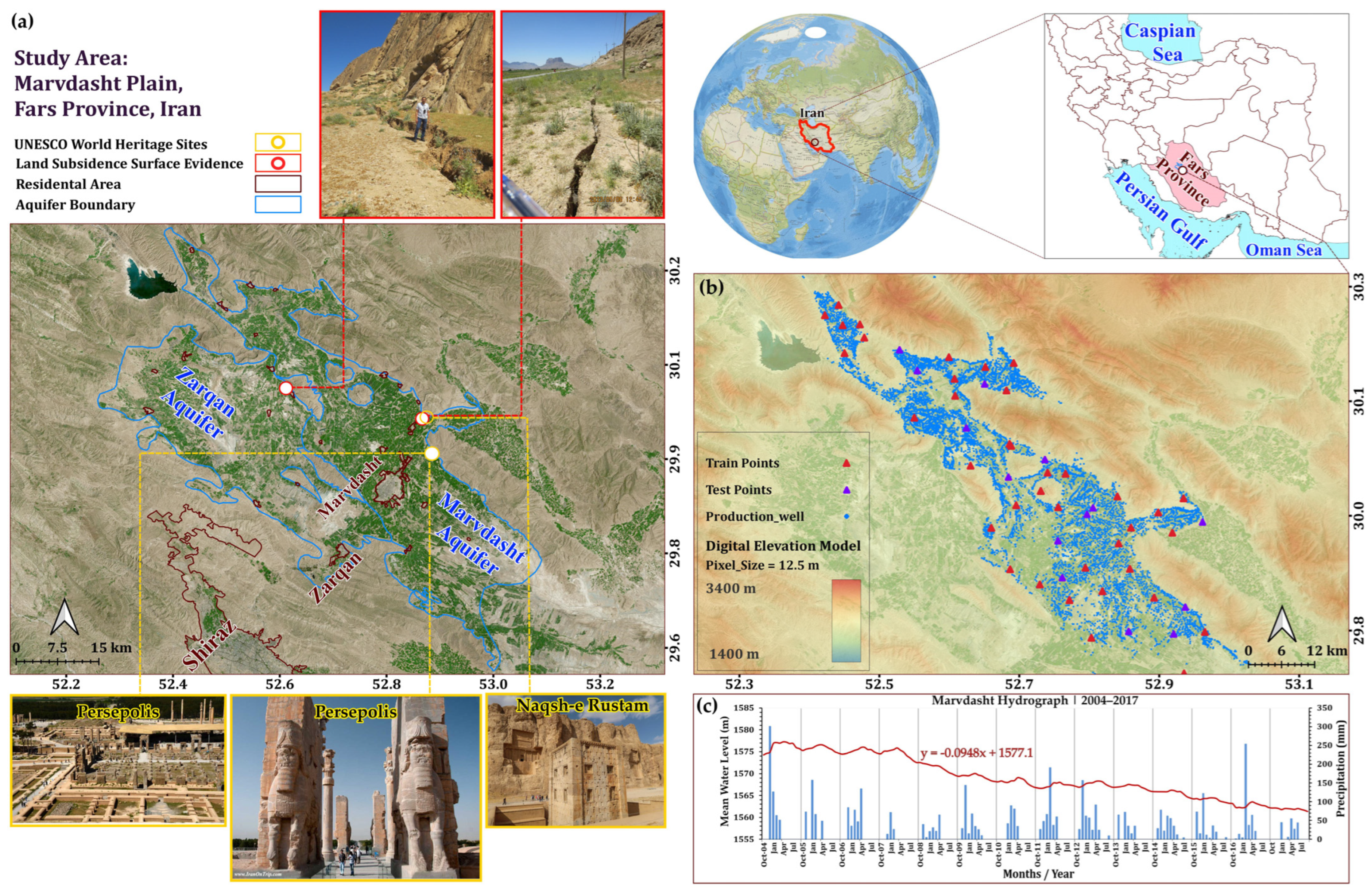
2. Study Area Description

The Marvdasht Plain in Fars Province, Iran, home to the UNESCO World Heritage Site of Persepolis and the ancient rock reliefs of Naqsh-e Rustam [29,30,31] (Figure 1a), faces critical challenges from groundwater overexploitation and resulting land subsidence.

Scientific explorations and excavations conducted in various hills of the Marvdasht plain indicate that thousands of years before Darius the Great chose the rocky hill at the foot of Mount Rahmat to build his grand palaces, civilized peoples had lived and cultivated in its vast plain [32]. Owing to favorable geographical conditions, including abundant water and fertile land, this region enjoyed a strong economic status. However, the Marvdasht Plain now confronts significant threats due to unsustainable water management practices, with groundwater depletion reaching approximately 6 billion cubic meters annually [33]. This overexploitation has led to land subsidence, which affects about 56,000 km² of Iran, with some areas experiencing rates exceeding 10 cm/year [34]. The region’s historical significance and agricultural potential are at risk as aquifers continue to deplete.

Agriculture in this area is carried out both industrially and traditionally, using both dry farming and irrigation methods, using more than 8000 exploitation wells (Figure 1b). The extensive agricultural lands of this region are divided into seven homogeneous areas with similar characteristics, covered by seven rural agricultural service centers and 13 rural production cooperatives. In 1995, Marvdasht County produced 215,000 tons of wheat, and by 2001–2002, wheat production had reached 304,000 tons, earning the county the top position in wheat production. Marvdasht has 170,000 hectares of agricultural land, including 148,000 hectares of irrigated land and 22,000 hectares of dry farmland. However, excessive irrigation practices have made the plain particularly vulnerable to groundwater depletion and land subsidence [34,35]. The region’s main agricultural products include irrigated wheat and barley, rice, sugar beets, grain corn, and fodder corn, with melon fields covering the largest cultivated area. Given sufficient water resources, the region is also well-positioned for horticulture. It is worth mentioning that the water required for agriculture and horticulture in the region is supplied from wells, qanats, and rivers.

Geological and Hydrogeological Information

The Marvdasht Plain forms part of a large intermontane basin within the Zagros Mountain chain, which extends in a northwest-southeast direction. This basin resulted from the collision of the Arabian and Eurasian plates [36,37,38]. The study area lies within the crush zone of the main Zagros thrust. Tectonic processes, including faulting and folding, have shaped the region, producing fractured limestone units that serve as natural groundwater reservoirs. These units are mostly concealed beneath Quaternary alluvial deposits [39]. The plain is surrounded by several mountain ranges: the Zagros Mountains to the west and northwest, Kuh-e Rahmat to the east, Kuh-e Hossein to the northeast, and Kuh-e Tasuj to the southeast. These ranges consist of diverse rock types, including limestone, marl, shale, metamorphic rocks, and igneous intrusions [40]. The geology of the Marvdasht Plain, as depicted in Figure 2, encompasses formations spanning the Cretaceous to the Tertiary. These formations significantly influence the region’s structural and hydrogeological characteristics. The Sarvak, Asmari, Jahrom, and Daryan formations constitute the primary bedrock aquifers. Composed of thick-bedded, sometimes dolomitized limestones, these formations have developed into major karst aquifers due to extensive fracturing and jointing. In contrast, the Gachsaran formation, consisting of marl, gypsum, and salt, exhibits low permeability and acts as an aquitard, impeding vertical water movement. Quaternary sediments, derived from surrounding sedimentary rocks, cover most of the study area. These sediments include loess, loess-like deposits, and alluvial materials ranging in texture from fine to coarse—gravel, sand, silt, and clay [41,42]. Deposited by fluvial and lacustrine systems, these materials have created fertile soils that sustain the region’s rich agricultural and cultural heritage. Notably, Cretaceous limestone formations, particularly the Sarvak Formation, function as key aquifer units, represented by $K_{sr}^{l.m}$ layer in A-A+ and B-B+ geology sections (Figure 2). A confined aquifer system underlies the Marvdasht Plain, with Quaternary alluvium and fractured limestone forming the primary aquifers, while marl and shale serve as aquitards [43].

Excessive groundwater extraction has triggered a significant decline in water levels, as shown in Figure 1c. From approximately 1577 m in October 2004, the water level dropped to around 1562 m by October 2017—a decrease of about 15 m over 13 years. A red dashed trendline in the hydrograph, with the equation y = −0.0948x + 1577.1 (where x is time in months), quantifies this decline at a rate of roughly 0.0948 m per month or 1.154 m per year. This significant decline in groundwater level has led to the compaction of clay-rich layers, resulting in land subsidence across the Marvdasht Plain [44,45]. Precipitation data, shown as blue bars along the x-axis, reflect the semi-arid climate of Fars Province. Peaks occur during the wet season (November to March), with maximum monthly values reaching approximately 300 mm. Nevertheless, most months exhibit minimal or no precipitation, mainly during the dry season (April to October). The limited recharge from these sporadic events fails to offset the continuous groundwater withdrawal, as evidenced by the lack of significant groundwater level recovery following precipitation peaks. This imbalance underscores the unsustainable water management practices in the region. The hydrograph provides a temporal dimension to the spatial data in Figure 1a,b, quantifying the rate and extent of aquifer decline. It serves as a critical metric for this study, supporting the use of remote sensing and modeling to monitor and predict groundwater level trends, which are essential to understanding the geological and hydrogeological framework. Consequently, a comprehensive understanding of the geological and hydrogeological framework of the Marvdasht Plain is vital for devising strategies to mitigate land subsidence and preserve the region’s historic landmarks.

3. Materials and Methods

3.1. Data Acquisition

Sentinel-1 Single Look Complex (SLC) products are distributed by the European Space Agency (ESA). These products are acquired by a pair of sun-synchronous, polar-orbiting satellites that operate in the same orbital plane but are positioned 180° apart, ensuring continuous coverage. The satellites conduct all-weather, day-and-night observations using C-band synthetic aperture radar (SAR). Sentinel-1 operates in four exclusive imaging modes—Stripmap, Interferometric Wide Swath, Extra Wide Swath, and Wave—offering spatial resolutions as fine as 5 m and swath widths up to 400 km (

Table 1. Sentinel-1 specifications for InSAR time series land subsidence.

Parameters	Specifications
Resolution	5 × 20 m
Band type	C-band
Orbit height	693 km
Orbit inclination	98.18°
Temporal coverage	12 days (12/2014 to 12/2022)/6 days (12/2014 to 12/2022)
Spectral range	3.75–7.5 cm
Mode	Interferometric Wide (IW)

). The mission supports dual polarization, delivers frequent revisit times, and ensures rapid product availability. Each acquisition includes high-precision measurements of the satellite’s position and altitude. A pre-programmed observation strategy ensures data consistency over time, making Sentinel-1 especially well-suited for long-term applications such as land subsidence monitoring.

Table 2. Dataset description.

Variable Name	Source (Webpage, Accessed Date)	Units	Spatial Resolution
Terrain Aspect	https://zenodo.org/records/15689805, accessed on 20 November 2024	Degrees (0–360°)	30 m
Digital Elevation Model (DEM)	https://www.earthdata.nasa.gov/, accessed on 20 November 2024	Meters (m)	30 m
Slope	https://www.earthdata.nasa.gov/, accessed on 20 November 2024	Degrees (°)	30 m
Ground Deformation Time Series	https://dataspace.copernicus.eu/, accessed on 20 November 2024	Millimeters yr−1	10 m
Potential Evapotranspiration (PET)	https://www.earthdata.nasa.gov/data/, accessed on 20 November 2024	mm day−1	500 m
Precipitation (CHIRPS)	https://www.chc.ucsb.edu/data/chirps, accessed on 20 November 2024	Millimeters (mm)	~5 km
Terrestrial Water Storage Anomaly (GRACE)	http://grace.jpl.nasa.gov/, accessed on 20 November 2024	cm water-eq.	55 km
Soil Moisture	https://nsidc.org/data/smap, accessed on 20 November 2024	m3 m−3	9 km
Surface Air Temperature	https://cds.climate.copernicus.eu/, accessed on 20 November 2024	Kelvin (K)	31 km
Land Surface Temperature (LST)	https://www.earthdata.nasa.gov/data, accessed on 20 November 2024	Kelvin (K)	1 km
Atmospheric Humidity	https://cds.climate.copernicus.eu/, accessed on 20 November 2024	Percent (%)	31 km
Enhanced Vegetation Index (EVI)	https://www.earthdata.nasa.gov/data/, accessed on 20 November 2024	Dimensionless (–1–+1)	500 m
Normalized Difference Vegetation Index (NDVI)	https://www.earthdata.nasa.gov/data/, accessed on 20 November 2024	Dimensionless (–1–+1)	500 m
Fraction of Photosynthetically Active Radiation (FPAR)	https://www.earthdata.nasa.gov/data/, accessed on 20 November 2024	Fraction (0–1)	500 m
Leaf Area Index (LAI)	https://www.earthdata.nasa.gov/data/, accessed on 20 November 2024	m2 m−2	500 m
Normalized Difference Water Index (NDWI)	https://www.earthdata.nasa.gov/data/, accessed on 20 November 2024	Dimensionless (–1–+1)	500 m
Gross Primary Productivity (GPP)	https://www.earthdata.nasa.gov/data/, accessed on 20 November 2024	g C m−2 day−1	500 m
Sand Fraction	https://stac.openlandmap.org/, accessed on 20 November 2024	Percent (%)	250 m
Clay Fraction	https://stac.openlandmap.org/, accessed on 20 November 2024	Percent (%)	250 m
Bulk Soil Organic Carbon (SOC)	https://stac.openlandmap.org/, accessed on 20 November 2024	kg C m−2	250 m

presents a summary of the multi-domain datasets employed to model groundwater dynamics, integrating geomorphological (e.g., DEM, slope), hydroclimatic (e.g., terrestrial water storage anomaly (TWSA) from GRACE and precipitation), biophysical (e.g., NDVI and LAI), and geophysical (e.g., InSAR-derived deformation) variables [46,47,48]. These datasets were obtained from various sources, including NASA (MOD11A2 and MODIS), the USGS (SRTM), ESA Copernicus, and in situ monitoring networks. Spatial resolutions range from 30 m (e.g., DEM) to 0.1° (e.g., GRACE), while temporal resolutions span from daily (e.g., precipitation) to monthly (e.g., deformation) intervals [49]. All variables were harmonized in terms of units and data formats to support cross-domain machine learning workflows. Key proxies such as GRACE-TWSA and soil moisture, along with InSAR-derived deformation time series, provide direct insights into subsurface hydrological processes [50,51,52]. To derive surface deformation time series, imagery from the Sentinel-1 constellation was utilized. Moreover, we also utilize information from the Open Land Map, including soil types (clay, sand, bulk density, and soil organic carbon).

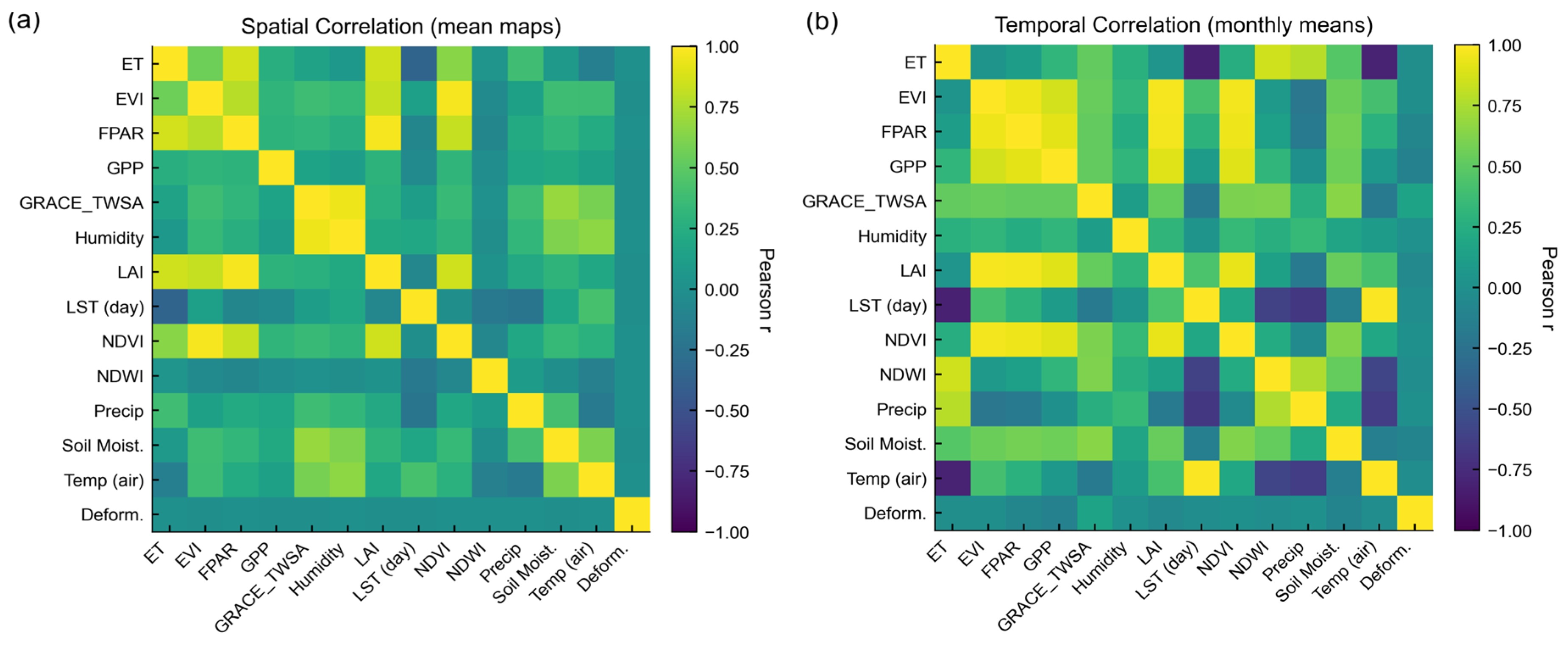
Dataset Spatial and Temporal Correlation

Figure 3 presents the spatial (a) and temporal (b) correlations between hydrometeorological covariates, terrain forms, and auxiliary datasets using Pearson correlation coefficients. The matrix reveals significant positive correlations between soil moisture, NDWI, precipitation, and deformation data, highlighting their robust potential for capturing groundwater fluctuations [53,54]. Notably, soil moisture and NDWI are particularly effective in reflecting changes in surface and subsurface water availability, indicating their importance in groundwater level predictions [55].

Vegetation indices such as NDVI, EVI, and FPAR exhibit strong seasonal correlations with precipitation and soil moisture, capturing the impact of climatic variability on groundwater recharge dynamics [56,57,58]. Additionally, temperature and LST show moderate negative correlations with deformation data, suggesting potential subsidence in areas with groundwater depletion [59,60]. These findings emphasize the relevance of integrating vegetation parameters, soil moisture, and surface deformation data as critical predictors for groundwater variation analysis, given their pronounced responses to seasonal and climatic variations.

Moreover, 54 piezometric boreholes were installed across the Naqsh-e Rustam-Persepolis-Marvdasht aquifer system, a semi-arid region underlain by calcareous soils (limestone-dominant), alluvial deposits, and clay-rich Quaternary sediments. Boreholes were split into training (70%) and testing (30%), preserving hydrostratigraphic representation (e.g., Bakhtiari Conglomerate and Asmari Formation). Training sites focused on agriculturally intensive zones with high irrigation-linked groundwater variability, while test sites targeted peripheral areas with sparse monitoring. The partitioning ensures model generalizability across heterogeneous lithologies critical to regional groundwater dynamics; the spatial location of those piezometers is presented in Figure 1b.

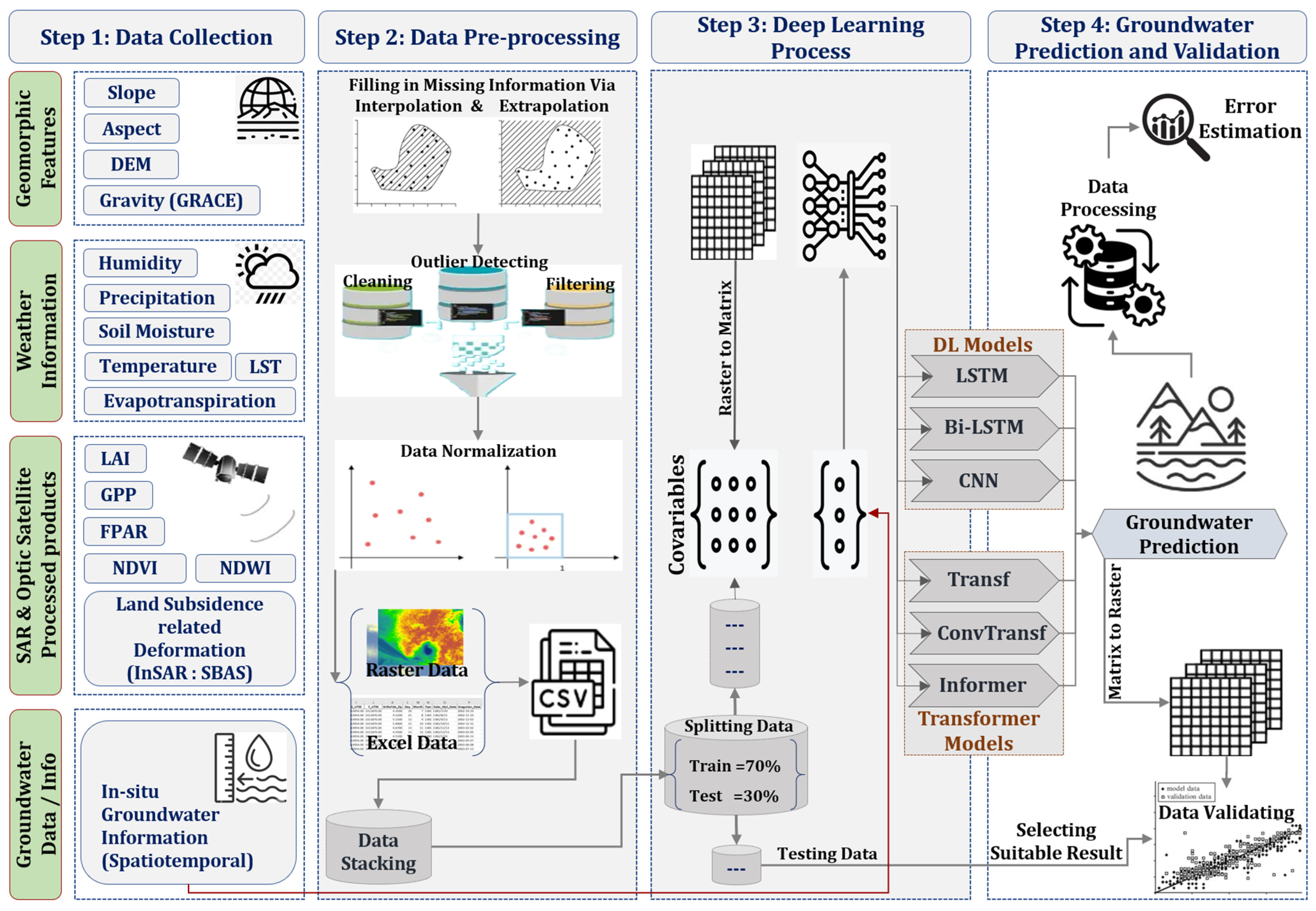
3.2. Methodology Framework

This study integrates multisource geospatial, meteorological, and hydrological data to model groundwater variations using deep learning techniques. The entire methodology workflow is presented in Figure 4. As indicated above, data collection encompasses geomorphic parameters (slope, aspect, DEM, and GRACE gravity data), meteorological variables (precipitation, temperature, humidity, evapotranspiration, land surface temperature, and soil moisture), spectral indices (NDVI, GPP, NDWI, LAI, and FPAR), displacement rate (land subsidence), and in situ groundwater measurements. These datasets, spanning multiple temporal resolutions, provide a comprehensive foundation for subsequent analysis.

Pre-processing involves data cleaning, interpolation of missing values, normalization, and feature selection to ensure consistency across diverse data sources. Structured datasets are compiled in standardized formats and partitioned into training and testing subsets. Raster data are transformed into a matrix representation to facilitate integration with auxiliary variables. This step ensures that all input features are optimized for deep learning and transformer models while preserving their spatial and temporal integrity.

InSAR time series analysis is conducted using the SBAS approach to derive ground deformation patterns indicative of subsurface hydrological variations. Deformation maps are extracted and combined with ancillary datasets to serve as covariates in predictive modeling. The processed data are subsequently utilized to train deep learning models, including LSTM, Bi-LSTM, CNN-LSTM, Transformer, ConvTransformer, and Informer. These models capture spatiotemporal dependencies, enabling high-accuracy groundwater level predictions. The final stage involves data validation, model performance assessment, and spatiotemporal prediction of groundwater fluctuations. Based on validation metrics, the most robust model outputs are selected, followed by visualization and interpretation of results. Predicted groundwater trends are analyzed in conjunction with environmental and climatic variables to derive insights into subsurface water dynamics. This integrated methodology supports the potential of deep learning and InSAR synergy for groundwater monitoring and sustainable water resource management.

3.2.1. Data Processing

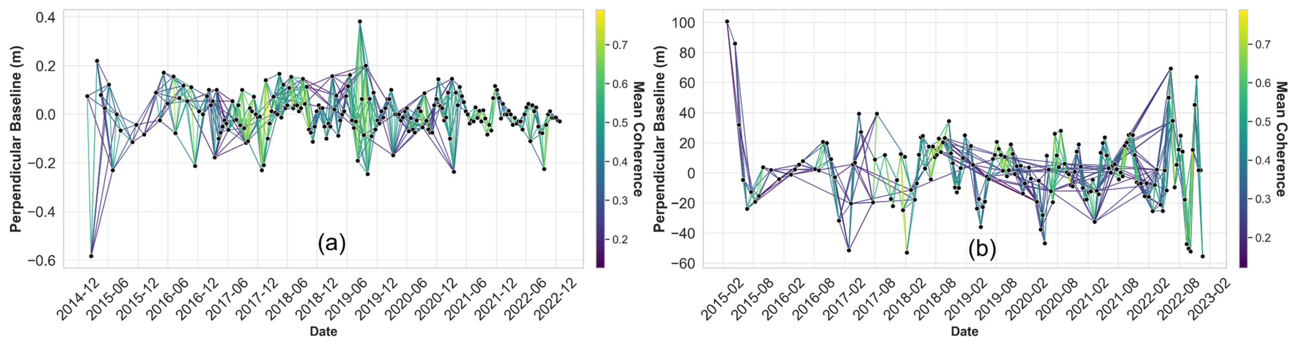
SAR Data Processing

To quantify ground displacement across the study area from January 2015 to December 2022, we processed 432 C-band Sentinel-1 Synthetic Aperture Radar (SAR) images, comprising 234 ascending- and 198 descending-orbit acquisitions. The Sentinel-1 Single Look Complex (SLC) products, provided by the European Space Agency (ESA), undergo pre-processing such as instrument processing facility (IPF) that includes mitigation of Radio Frequency Interference (RFI) to ensure data quality [61]. The dual-orbit strategy aimed to (i) mitigate SAR geometrical distortions (e.g., layover and shadowing) and (ii) cross-validate displacement estimates and land subsidence identifications through multi-geometry analysis. Employing the Small Baseline Subset (SBAS) technique via the LiCSBAS package [62], we generated interferometric pairs using maximum spatial baselines of 100 m (ascending) and 200 m (descending). Interferograms were multi-looked with a 4:1 (range: azimuth) ratio to enhance phase stability, achieving detection thresholds for slope movements as small as 100 m spatially. After filtering noisy unwrapped phases, displacement time series were reconstructed from high-coherence interferometric pairs, with each epoch linked to 3–4 temporally adjacent SAR scenes. The LiCSBAS workflow includes quality control measures, such as coherence-based selection and phase filtering, which further minimize the impact of any residual noise, including potential RFI effects. Temporal coherence degradation was observed during two intervals: (i) post-December 2021, following Sentinel-1B’s orbital retirement, and (ii) mid-June to July 2019 due to ascending data gaps. The spatiotemporal baseline configuration of the SBAS network is illustrated in Figure 5a (ascending) and Figure 5b (descending).

A common decomposition (assuming eastward and vertical motion dominate or ignoring the north component if geometry and data availability permit) is as follows:

$${\mathrm{v}}_{\mathrm{a}\mathrm{s}\mathrm{c}}={\mathrm{v}}_{\mathrm{x}}·\mathrm{s}\mathrm{i}\mathrm{n}{\mathsf{\theta }}_{\mathrm{a}\mathrm{s}\mathrm{c}}·\mathrm{c}\mathrm{o}\mathrm{s}{\mathsf{\alpha }}_{\mathrm{a}\mathrm{s}\mathrm{c}}+{\mathrm{v}}_{\mathrm{y}}·\mathrm{s}\mathrm{i}\mathrm{n}{\mathsf{\theta }}_{\mathrm{a}\mathrm{s}\mathrm{c}}·\mathrm{s}\mathrm{i}\mathrm{n}{\mathsf{\alpha }}_{\mathrm{a}\mathrm{s}\mathrm{c}}+{\mathrm{v}}_{\mathrm{z}}·\mathrm{c}\mathrm{o}\mathrm{s}{\mathsf{\theta }}_{\mathrm{a}\mathrm{s}\mathrm{c}}$$

(1)

$${\mathrm{v}}_{\mathrm{d}\mathrm{e}\mathrm{s}\mathrm{c}}={\mathrm{v}}_{\mathrm{x}}·\mathrm{s}\mathrm{i}\mathrm{n}{\mathsf{\theta }}_{\mathrm{d}\mathrm{e}\mathrm{s}\mathrm{c}}·\mathrm{c}\mathrm{o}\mathrm{s}{\mathsf{\alpha }}_{\mathrm{d}\mathrm{e}\mathrm{s}\mathrm{c}}+{\mathrm{v}}_{\mathrm{y}}·\mathrm{s}\mathrm{i}\mathrm{n}{\mathsf{\theta }}_{\mathrm{d}\mathrm{e}\mathrm{s}\mathrm{c}}·\mathrm{s}\mathrm{i}\mathrm{n}{\mathsf{\alpha }}_{\mathrm{d}\mathrm{e}\mathrm{s}\mathrm{c}}+{\mathrm{v}}_{\mathrm{z}}·\mathrm{c}\mathrm{o}\mathrm{s}{\mathsf{\theta }}_{\mathrm{d}\mathrm{e}\mathrm{s}\mathrm{c}}$$

(2)

One way to solve explicitly for $v_z$ and (for instance) $v_x$ is by arranging these equations in matrix form or by applying known trigonometric simplifications [63,64]. A frequently cited simplified pair (assuming motion is primarily east ($v_x$) and vertical ($v_z$)) is as follows:

$$\left[\begin{array}{c}{\mathrm{v}}_{\mathrm{a}\mathrm{s}\mathrm{c}}\\ {\mathrm{v}}_{\mathrm{d}\mathrm{e}\mathrm{s}\mathrm{c}}\end{array}\right]=\left[\begin{array}{c}\sin {\mathsf{\theta }}_{\mathrm{a}\mathrm{s}\mathrm{c}}·\cos {\mathsf{\alpha }}_{\mathrm{a}\mathrm{s}\mathrm{c}} \cos {\mathsf{\theta }}_{\mathrm{a}\mathrm{s}\mathrm{c}}\\ \sin {\mathsf{\theta }}_{\mathrm{d}\mathrm{e}\mathrm{s}\mathrm{c}}·\cos {\mathsf{\alpha }}_{\mathrm{d}\mathrm{e}\mathrm{s}\mathrm{c}} \cos {\mathsf{\theta }}_{\mathrm{d}\mathrm{e}\mathrm{s}\mathrm{c}}\end{array}\right]\left[\begin{array}{c}{\mathrm{v}}_{\mathrm{x}}\\ {\mathrm{v}}_{\mathrm{z}}\end{array}\right]$$

(3)

One can invert this 2 × 2 system (when the look angles differ sufficiently) to isolate $v_x$ and $v_z$. For more general 3D decompositions (east, north, and up), additional constraints or multi-orbit data (multiple incidence/azimuth angles) are typically required [65,66]. This combination of velocities allows us to calculate vertical velocity for our analysis.

3.2.2. Models’ Architecture

LSTM; BiLSTM; CNN_LSTM; Transformer Multi-head self-attention layers, positional encoding for temporal sequence order, and feed-forward layers for feature extraction; ConvTransformer that combines CNN layers (for spatial pattern extraction) with Transformer attention layers to effectively integrate spatial-temporal dependencies; and Informer that employs probabilistic sparse attention mechanisms, significantly reducing computational complexity for long-sequence predictions.

All of these methods are employed in this pipeline for time series prediction. LSTM and BiLSTM are effective in capturing long-term dependencies in sequential data by using memory cells and bidirectional processing [66]. CNN-LSTM integrates convolutional layers to extract spatial features, followed by LSTM to capture temporal dependencies, thus enhancing spatial-temporal learning [67]. Transformers utilize self-attention mechanisms to effectively handle long-range dependencies, making them suitable for complex time series prediction [68]. ConvTransformer combines CNN for spatial learning with Transformer for sequence processing, while Informer optimizes the Transformer architecture by focusing on key information, thus reducing computational complexity. Each model is specifically described in

Table 3. Models’ architecture.

Model	Architecture	Key Hyperparameters
LSTM	1. Input: L × d sequence	• u1, u2 ∈ {32, 64, 128}
	2. LSTM (units = u1, return_sequences = True)	• dr ∈ {0.1, 0.2, 0.3}
	3. Dropout (rate = dr)	• Learning rate ∈ {1 × 10−4, 5 × 10−4, 1 × 10−3}
	4. LSTM (units = u2)
	5. Dense (1)
BiLSTM	1. Input: L × d sequence	• u ∈ {32, 64, 128}
	2. Bidirectional LSTM (units = u)	• dr ∈ {0.1, 0.2, 0.3}
	3. Dropout (rate = dr)	• Learning rate ∈ {1 × 10−4, 5 × 10−4, 1 × 10−3}
	4. Dense (1)
CNN–LSTM	1. Input: L × d sequence	• f, u ∈ {32, 64, 128}
	2. Conv1D (filters = f, kernel_size = 3, padding = “causal”, activation = ReLU)	• dr ∈ {0.1, 0.2, 0.3}
	3. Dropout (rate = drd)	• Learning rate ∈ {1 × 10−4, 5 × 10−4, 1 × 10−3}
	4. LSTM (units = u)
	5. Dense (1)
Transformer	1. Input: L × d sequence	• d ∈ {32, 64, 128}
	2. Dense to model-dim d + Add pos-enc	• heads ∈ {2, 4}
	3. Repeat n×:	• n ∈ {1, 2}
	3.1. MultiHeadAttention (heads = h, key_dim = d/h) → Add and LayerNorm	• dr ∈ {0.1, 0.2, 0.3}
	3.2. FFN: Dense(4d)→ReLU→Dense(d) → Add and LayerNorm	• Learning rate ∈ {1 × 10−4, 5 × 10−4, 1 × 10−3}
	4. GlobalAveragePooling1D
	5. Dense (1)
ConvTransformer	1. Input: L × d sequence	• f, d ∈ {32, 64, 128}
	2. Conv1D (filters = f, kernel_size = 3, padding = “same”, activation = ReLU)	• heads ∈ {2, 4}
	3. Dense to model-dim d + Add pos-enc	• n∈ {1, 2}
	4. Repeat n×: same TX stack as Transformer	• dr ∈ {0.1, 0.2, 0.3}
	5. GlobalAveragePooling1D	• Learning rate ∈ {1 × 10−4, 5 × 10−4, 1 × 10−3}
	6. Dense (1)
Informer	1. Input: L × d sequence	• d ∈ {32, 64, 128}
	2. Dense to model-dim d + Add pos-enc	• heads ∈ {2, 4}
	3. Repeat n×: same TX stack as Transformer (ProbSparse self-attention)	• n ∈ {1, 2}
	4. GlobalAveragePooling1D	• dr ∈ {0.1, 0.2, 0.3}
	5. Dense (1)	• Learning rate ∈ {1 × 10−4, 5 × 10−4, 1 × 10−3}

, along with their hyperparameter variations to enhance the accuracy of our results and have an effective training process.

3.2.3. Training Pre-Processing

The data pre-processing stage involves the transformation of raw covariate raster stacks and station data into structured input sequences for model training. The target variable is s, and covariates include 95-band raster data for multiple features over the 2015–2023 period. The data are scaled tile-wise using the StandardScaler method:

$$X_{norm}=X-\mathsf{\mu }/\mathsf{\sigma }$$

(4)

where $X$ is the raw feature matrix, $\mathsf{\mu }$ is the mean of the training data, and σ is the standard deviation of the training data. The input tensor $X$ is structured as sequences with 95 features (that correspond to 95 five-monthly layers) per timestep:

$$X_{seq}=\left[x_t,x_{t+1},\dots ,x_{t+11}\right]$$

(5)

For each station, covariate values are sampled using raster indices derived from latitude and longitude, transformed using the raster transform matrix:

$$\left(r,c\right)=T^{-1}\times \left(lon,lat\right)$$

(6)

3.2.4. Prediction Process

The prediction pipeline processes tiled raster data, reducing memory overhead. The scaled input tensors are processed through the trained models to generate predictions. The output is restructured into raster format using the inverse transformation:

$$X_{pred}=X_{norm}\times \sigma +\mathsf{\mu }$$

(7)

3.2.5. Error Evaluation

This metric quantifies the proportion of variance in the observed groundwater levels that is explained by the model predictions [2]. It is defined as follows:

$$R^2=1-{\displaystyle \frac{{\sum }_{i=1}^n{\left(y_{obs,i}-y_{pred,i}\right)}^2}{{\sum }_{i=1}^n{\left(y_{obs,i}-\overline{y_{obs}}\right)}^2}}$$

(8)

RMSE provides the magnitude of average prediction errors, emphasizing larger errors due to squaring [19]. It is calculated by:

$$\mathrm{RMSE}=\sqrt{{\displaystyle \frac{1}{n}}\sum _{i=1}^n{\left(y_{pred,i}-y_{obs,i}\right)}^2}$$

(9)

MAE indicates the average absolute prediction error without emphasizing outliers [12]. It is expressed as follows:

$$\mathrm{MAE}={\displaystyle \frac{1}{n}}\sum _{i=1}^n\left|y_{pred,i}-y_{obs,i}\right|$$

(10)

MAPE quantifies prediction accuracy as an average percentage error [19] useful for normalized error comparison:

$$\mathrm{MAPE}={\displaystyle \frac{100}{n}}\sum _{i=1}^n\left|{\displaystyle \frac{y_{pred,i}-y_{obs,i}}{y_{obs,i}}}\right|$$

(11)

This metric measures the strength and direction of linear association between observed and predicted groundwater levels:

$$r={\displaystyle \frac{{\sum }_{i=1}^n\left(y_{obs,i}-\overline{y_{obs}}\right)\left(y_{pred,i}-\overline{y_{pred}}\right)}{\sqrt{{\sum }_{i=1}^n{\left(y_{obs,i}-\overline{y_{obs}}\right)}^2\sqrt{{\sum }_{i=1}^n{\left(y_{pred,i}-\overline{y_{pred}}\right)}^2}}}}$$

(12)

Moreover, an evaluation based on the Taylor diagram is presented to visualize model performance by combining correlation, standard deviation, and RMSE. It enables clear comparison of deep learning and transformer models in capturing groundwater variability.

4. Results and Discussion

4.1. Model’s Performance

This section presents the study’s results, focusing on ground displacement analysis using InSAR and deep learning model performance. Using the SBAS technique, interferometric pairs were generated, revealing subsidence patterns linked to groundwater withdrawal. Deep learning models, including LSTM and CNN, were evaluated for spatiotemporal groundwater level prediction, with metrics like R² and RMSE analyzed. Temporal groundwater trends highlighted significant depletion and localized subsidence near key archaeological sites, emphasizing the need for sustainable management to preserve these heritage areas.

Figure 6 provides an integrated evaluation of environmental variable importance, model performance, and training stability across multiple deep learning models for groundwater level prediction. Velocity, NDVI, GPP, and aspect emerge as dominant covariates, collectively explaining 51.2% of predictive power, while secondary variables including DEM, slope, and deformation contribute an additional ~24.9%. The ConvTransformer clearly leads the pack, posting an R² of ≈0.83, an MAE of ≈3 m, an RMSE of ≈6 m, and a MAPE below 2%. It outperforms the vanilla Transformer (R² ≈ 0.69, MAE ≈ 6 m) and decisively eclipses Informer, whose accuracy drops to R² ≈ 0.35 and MAE ≈ 9 m. The recurrent baselines—LSTM, BiLSTM, and CNN-LSTM—occupy the middle ground, with R² values of roughly 0.45–0.60 and MAEs in the 5–8 m range.

Training dynamics highlight the efficiency of attention-based models, with Informer, Transformer, and ConvTrans achieving stable and low validation losses around 0.08–0.09 after approximately 120 epochs, whereas recurrent models exhibit higher loss (~0.18) with noticeable overfitting. Error distributions underscore these differences, with Informer and Transformer capturing approximately 90% of predictions within ±20 m, compared to only ~60% for CNN-LSTM. Overall, attention-based neural networks indicate substantial accuracy improvements by efficiently leveraging critical environmental features.

4.2. Hyperparameter Calibration

Figure 7 systematically evaluates the validation loss landscape across six distinct sequential deep learning architectures—LSTM, Bi-LSTM, CNN-LSTM, ConvTransformer, Transformer, and Informer—to optimize predictions. Each model’s hyperparameters were rigorously tuned through extensive experimentation. In the LSTM model, validation loss is minimized (~0.75) at moderate complexity: first-layer hidden units (u1) at 32–128 and second-layer units (u2) at 64–128, with optimal dropout rate (dr) around 0.2. Excessive regularization (dr = 0.3) or overly large hidden layers sharply elevate loss toward 0.88. The Bi-LSTM, characterized by its single hidden-layer parameter (u2), achieves its lowest validation loss (~0.83) at u2 = 128 units with a modest dr = 0.1, but performance significantly deteriorates with increased dropout (dr ≥ 0.3).

The hybrid CNN-LSTM architecture, combining convolutional layers (filters, f = 32–64) and recurrent units (lstm_u = 32–128), exhibits the lowest loss (~0.86) at f = 64, lstm_u = 128, and dr = 0.1. Any deviation towards smaller LSTM units (lstm_u = 32) or higher dropout significantly escalates validation loss beyond 0.99, underscoring the sensitivity of this model configuration. For the ConvTransformer, embedding dimensions (d = 64–128), attention heads (2–4), and layers (1–2) yield optimal validation loss (~0.68) when using intermediate settings (d = 64, heads = 2, layers = 2, dr = 0.3). Increased embedding dimensions without sufficient regularization quickly inflate the validation loss (>0.70). In contrast, the vanilla Transformer architecture achieves its lowest validation loss (~0.72) with maximal model complexity (d = 128, heads = 4, layers = 2) and minimal dropout (dr = 0.1), emphasizing the importance of carefully balancing capacity with regularization.

Finally, the Informer—a specialized transformer variant optimized for temporal modeling—records the minimal validation loss (~0.79) with parameters set at moderate complexity (d = 128, heads = 2, and layers = 2) and the highest evaluated dropout (dr = 0.3). However, smaller embeddings or fewer attention heads rapidly increase the loss above 0.88. Collectively, this analysis reveals a clear trend across models: a nuanced balance between model capacity (embedding dimensions and hidden units), moderate regularization (dr = 0.1–0.3), and controlled learning rates is essential to achieve optimal predictive performance. These insights provide a rigorous, empirically driven guideline for future hyperparameter selections in sequential deep learning architectures for hydrological forecasting.

4.3. Validation

Figure 8 presents nine representative time series of monthly groundwater level elevations recorded in situ (solid black) along with predictions from six deep learning architectures. The observed wells span three characteristic hydrogeologic regimes: (1) nearly flat plateaus in confined alluvial settings (e.g., Station 28 and Station 11), (2) slow, persistent seasonal drawdowns on fractured piedmonts (e.g., Station 20 and Station 47), and (3) strongly modulated responses in irrigated lowlands with double-peaked recharge signals (e.g., Station 23 and Station 6). All series exhibit pronounced minima during peak evapotranspiration each summer and sharp rises following major recharge events, providing a stringent testbed for model fidelity.

Among the six predictors, the Transformer (yellow dash–dot) and ConvTransformer (teal dash–dot) consistently deliver the closest match to the black in situ curves across all nine wells. The pure Transformer captures both the long-term trends and the precise timing of seasonal troughs and rebounds, preserving amplitude without the phase lags or overshoot common to other methods. The ConvTransformer further refines this performance by reproducing short-term fluctuations and secondary peaks with minimal bias, even in the most dynamic lowland sites. In contrast, Informer (green dotted) tracks the broad strokes well but slightly underestimates extreme highs and lows; recurrent networks (BiLSTM and LSTM) drift in phase and amplitude over multi-year spans; and the CNN–LSTM hybrid smooths away much of the high-frequency variability. Together, these results highlight the superior skill of attention-only and convolution-augmented attention models—particularly Transformer and ConvTransformer—for operational groundwater monitoring.

In the following, the plots exhibit monthly groundwater level observations (1520–1625 m) against six model predictions, with point density contours (Figure 9). Each panel shows the 1:1 line (grey dashed) and an OLS fit (solid black), whose slope, intercept, and R² measure bias and scaling errors. Recurrent models (BiLSTM, LSTM, and CNN–LSTM) exhibit substantial scatter and departures from unity:

The BiLSTM model produces the regression line with the least steep slope (y = 0.86x + 220.86), low explanatory power (R² = 0.18), and largest spread (RMSE = 15.31 m, MAE = 10.68 m, MAPE = −0.5%), reflecting systematic under-prediction at the low end and over-prediction at the high end. CNN–LSTM nearly recovers unity (y = 0.96x + 59.04, R² = 0.44) and cuts RMSE to 12.45 m (MAE = 8.37 m, MAPE = −0.6%), but still shows clustered heteroscedastic deviations around the densest wells near 1560 m. LSTM improves R² to 0.59 (y = 0.87x + 201.59) and reduces RMSE further to 10.53 m (MAE = 7.16 m, MAPE = −0.7%), yet retains clear bimodal clouds corresponding to seasonal aquifer highs and lows.

In contrast, attention-enhanced architectures concentrate tightly around the 1:1 line: ConvTransformer is the best linear performer (y = 0.99x + 10.78, R² = 0.83), delivering the smallest errors (RMSE = 6.15 m, MAE = 3.92 m, MAPE = −0.9%) and virtually no bias across the range. The transformer slightly over-predicts at depth (y = 1.10x − 155.39) but still achieves R² = 0.71 with RMSE = 8.76 m (MAE = 6.02 m, MAPE = −0.8%), indicating strong fidelity except for extreme highs. Informer balances both worlds (y = 0.89x + 174.07, R² = 0.40, RMSE = 13.31 m, MAE = 9.07 m, MAPE = −0.6%), with a compact density kernel that minimizes systematic drift while retaining robustness to non-stationary signals. There is a visible slight overestimation in high water level areas; the main reason is the lack of data in those regions that are located in northern training points.

Together, these comparisons underscore that convolution-augmented attention (ConvTransformer) best aligns predictions to observations, while pure attention (Transformer and Informer) also outperforms recurrent variants by reducing scatter and extreme errors.

Figure 10 shows a Taylor diagram that the ConvTransformer (blue diamond) achieves the highest pattern correlation (r ≈ 0.91) against observed groundwater depths, with a model spread of σ ≈ 15 m and a centered RMS error of roughly 13 m. The pure Transformer (lime circle) comes next, registering r ≈ 0.83, σ ≈ 12 m, and CRMSE ≈ 12 m. The Informer (teal triangle) follows closely behind with r ≈ 0.80, σ ≈ 11 m, and CRMSE near 10 m. In contrast, the remaining architectures—CNN–LSTM, LSTM, and BiLSTM—fall farther from the target arc, reflecting their comparatively lower fidelity. Altogether, this ordering highlights the superior skill of the ConvTransformer’s convolution-augmented attention for regional hydrological forecasting.

A side-by-side comparison of each model’s spatial performance across the network of in situ wells is shown in Figure 11. In the left column (panels a–f), the LSTM row shows moderate correlations (r ≈ 0.6–0.8) but RMSEs that spike to ±40 m around basin margins, while BiLSTM (second row) tightens correlation slightly but still exhibits pockets of 30–50 m error. In this context, pockets refer to specific clusters of data points where the BiLSTM model’s error (standard deviation) is notably higher. The CNN–LSTM hybrid (third row) improves overall correlation to 0.5–0.9. Moving into pure attention, the Transformer (fourth row) yields correlations above 0.8 and reduces RMSE to 15 to −15 m, with only faint spatial bias around higher-elevation clusters. ConvTransformer (fifth row) further concentrates RMSE under ±5 m almost everywhere, matching or exceeding the Transformer’s correlation. Finally, the Pearson values are higher than 0.9 in almost all stations; the Informer (bottom row) uniformly achieves r > 0.80 and RMSE consistently within ±15 m, with virtually no geographic “hotspots” of error.

The right-hand Hovmöller panels reveal how each model’s residuals vary over time and latitude. LSTM, CNN-LSTM, and BiLSTM exhibit pronounced seasonal stripes; high value residuals are located in northern areas. The best residual values correspond to the ConvTransformer method.

4.4. Temporal and Spatial Groundwater Level Analysis

Figure 12 illustrates the temporal evolution of groundwater levels across 10 monitoring stations. The individual time series plots display ground displacement (blue line), groundwater level variations (red line), and precipitation levels (green bars). A consistent declining trend in groundwater levels is observed across all stations, with displacement rates varying depending on the location and the intensity of subsidence. The heatmap in the center highlights areas with the highest subsidence rates, reaching up to −180.9 mm/year, which aligns with regions experiencing the most significant groundwater depletion. The correlation between precipitation and groundwater fluctuations suggests that recharge periods are insufficient to counteract groundwater loss, leading to progressive subsidence. This subsidence results in threatening surface evidence, such as fissures located 10 m from the Naqsh-e Rustam complex (Figure 1a and Figure 13). These findings indicate that excessive groundwater extraction is a primary driver of surface deformation, particularly in the most affected zones.

The spatiotemporal evolution of the groundwater level across the study area from 2016 to 2022, revealing significant fluctuations over a 7-year period (Figure 14). The maps cover approximately 1816.12 km², spanning 29.7°N to 30.3°N latitude and 52.2°E to 52.8°E longitude, with groundwater elevations ranging from 1520 m to 1620 m.

The plain areas exhibit significant depletion, with average levels dropping by 10–15 m, and some locations—such as 29.9°N, 52.5°E—show a sharp decline from 1560 m in 2016 to 1535 m in 2022 (~25 m decrease). Conversely, mountainous regions maintain relatively stable levels near 1600 m, indicating their role as natural recharge zones. The northwestern section (30.2°N, 52.3°E) remains around 1600 m, exhibiting fluctuations within ±5 m, contrasting with the south-central plains, where declines exceed 20 m. The observed depletion trends align with increasing water demand, climate variability, and over-extraction, underscoring the urgent need for localized groundwater management. The consistency of results across multiple years confirms the reliability of the applied methodology, reinforcing its applicability for both small- and large-scale hydrogeological assessments, which are critical for ensuring long-term groundwater sustainability.

4.5. Comparative Analysis and Implications

This study advances groundwater level prediction by integrating remote sensing-derived land subsidence, spectral indices, and hydroclimatic variables within a ConvTransformer framework. By synthesizing insights from An et al. [19], Sun et al. [2], and Kulkarni et al. [48], we contextualize our contributions within the evolving landscape of spatiotemporal groundwater modeling. Our study addresses critical gaps in localized aquifer monitoring, particularly for culturally significant regions, while building upon recent methodological advancements. This discussion explores the evolution of predictive techniques, the unique integration of high-resolution data for heritage preservation, and the implications for sustainable resource management in semi-arid zones.

An et al. [19] illustrated the utility of GRACE-derived terrestrial water storage (TWS) and SAR-based deformation data for predicting groundwater storage (GWS) in Shanxi, China, using LSTM networks to capture large-scale temporal trends linked to climate variability. In contrast, our study integrates SBAS-InSAR-derived subsidence at 30 m resolution, enabling localized detection of aquifer stressors near UNESCO World Heritage Sites such as Persepolis and Naqsh-e Rustam. While GRACE provides valuable basin-scale TWS estimates, its coarse resolution (~1°) limits its applicability for heritage conservation. Our high-resolution subsidence feedback loops address this gap, extending the study of Haghshenas et al. [33] on InSAR-based aquifer compaction monitoring in Iran to predictive modeling for socio-environmental stewardship.

Sun et al. [2] validated the Transformer’s superiority over CNNs, LSTMs, and hybrid models for groundwater level prediction in Taiwan, emphasizing self-attention mechanisms for capturing long-term dependencies. Our ConvTransformer framework, combining spatial convolution with temporal attention, achieves comparable accuracy (R² ≈ 0.83) while explicitly modeling land subsidence feedbacks. Unlike Sun et al.’s station-based approach, our grid-level predictions reveal heterogeneous patterns driven by agricultural pumping and karst geology in the Marvdasht Plain. This spatially distributed modeling aligns with Chen et al.’s [12] recommendations for complex aquifers, particularly in data-scarce regions. Additionally, our use of attention weights to quantify uncertainty in high-prediction-error zones (e.g., fault-controlled aquifers) advances traditional LUBE methods [69], offering a dynamic framework for risk assessment.

Kulkarni et al. [48] conducted a multi-scale analysis of groundwater storage dynamics across North African basins, leveraging GRACE data, downscaled meteorological products, and land surface models to assess climate-driven variability. Their focus on large-scale climate teleconnections (e.g., North Atlantic Oscillation) contrasts with our high-resolution (30 m) predictions, which fuse SBAS-InSAR-derived subsidence with spectral and hydroclimatic covariates to capture anthropogenic stressors like agricultural pumping. While Kulkarni et al. [48] emphasized basin-scale climatic linkages, our approach bridges groundwater dynamics with surface deformation, addressing localized extraction impacts—a limitation of GRACE noted by Scanlon et al. [70].

A key strength of our study lies in its applicability to data-scarce heritage regions. Kulkarni et al. [48] highlighted remote sensing’s role in filling observational gaps in North Africa through GRACE downscaling and ERA5-Land reanalysis. Our framework complements this by integrating Sentinel-1 InSAR, Landsat NDWI, and CHIRPS precipitation data, providing a scalable solution for regions lacking dense hydrological networks, as advocated by Scanlon et al. [70]. However, similar to Sun et al.’s [2] observation of Transformer overfitting in multi-step forecasting, our model’s performance declines beyond three months (R² = 0.72 at T + 6), underscoring challenges in extrapolating nonlinear aquifer responses. Future studies could adopt Kulkarni et al.’s [48] multiscale strategy, coupling our ConvTransformer with GRACE-based TWS trends for cross-validation, as proposed by Wang et al. [50].

Our study’s integration of InSAR and transformer-based models represents a transformative step in hydrological modeling. SBAS-InSAR’s decadal archives enable retrospective analysis of aquifer depletion, complementing GRACE’s coarse-scale TWS trends [71]. The ConvTransformer’s capacity to detect precursory subsidence signals supports proactive groundwater governance in drought-prone regions, aligning with Riedel et al.’s [72] framework for climate change adaptation. By linking these advancements to UNESCO-relevant applications, our study bridges technical innovation with socio-environmental resilience. In summary, this study enhances groundwater prediction by addressing localized aquifer dynamics in culturally significant regions, filling gaps in prior large-scale or methodologically focused studies. Our high-resolution, attention-based framework not only improves prediction accuracy but also delivers actionable insights for heritage preservation and sustainable water management, marking a significant advancement in remote sensing and machine learning applications.

5. Conclusions

Our integration of SBAS-InSAR data with monthly multisource geoinformation layers provides the first sub-decadal (2015–2022) assessment of groundwater dynamics at a 30 m spatial resolution beneath the Persepolis and Naqsh-e Rustam UNESCO World Heritage complexes. Among the evaluated models, the convolution-enhanced Transformer demonstrates superior performance, explaining approximately 83% (R² ≈ 0.83) of the variance in blind-well validations and significantly reducing prediction errors to RMSE ≈ 6 m, MAE ≈ 4 m, and MAPE ≈ 12%. Compared to a CNN-LSTM baseline (RMSE ≈ 13 m; R² ≈ 0.44), this approach reduces prediction error by more than half, and compared to a vanilla LSTM model (R² ≈ 0.28), it nearly triples the variance explained. Furthermore, over 90% of absolute prediction errors remain below 15 m, with residuals closely distributed around zero. Conversely, the sparsity-optimized Informer explains only about 40% of the variance, retaining an RMSE greater than 13 m. This discrepancy highlights the effectiveness of dense convolutional attention mechanisms when modeling geophysically complex and high-dimensional time series. According to international guidelines, such as those from the International Council on Monuments and Sites (ICOMOS), land subsidence poses a significant threat to the structural integrity of stone heritage monuments, potentially causing irreversible cracking or collapse. Our observed and model-predicted subsidence rates exceeding 180 mm per year underscore a clear and immediate risk to the Persepolis stone carvings and associated heritage elements.

Across eight years of monthly observations, all Transformer variants—standard, convolutional, and sparse—consistently outperform recurrent architectures (LSTM, bi-LSTM, and CNN-LSTM) in terms of accuracy, bias, and residual structure. Multi-head self-attention preserves long-range dependencies without vanishing gradients, while sparse attention mechanisms scale efficiently across thousand-step horizons, an essential property for modeling long eco-hydrological archives. Feature attribution reveals that InSAR velocity, NDVI, GPP, and slope aspect jointly account for 51% of the model’s explanatory power, highlighting the importance of vegetation productivity and terrain morphology in encoding the hydrological memory needed for sustainable-use forecasting. Transformers effectively map these complex ecological signals to groundwater-level predictions with minimal phase drift by explicitly learning their latent couplings. This modeling framework enables early warning of cultural heritage risks by identifying subsidence hotspots exceeding –180 mm·yr⁻¹, which co-occur with groundwater storage losses of 4–6 m·yr⁻¹. Extrapolation suggests vertical displacement could exceed 200 mm·yr⁻¹ within a decade, posing a direct threat to the Achaemenid stone reliefs unless groundwater abstraction is significantly reduced. Attention-based saliency maps also highlight irrigation-induced stress periods that are obscured in recurrent baselines, facilitating transparent communication with water authorities.

Despite the robust performance of the proposed Transformer-based framework, several limitations warrant attention. First, while the dataset used for training covers a wide range of environmental variables, it may not fully capture the physical complexity of subsurface hydrology in the Marvdasht Plain. Second, InSAR-derived vertical motion was not directly validated with dense in situ measurements such as global navigation satellite system (GNSS) or extensometers due to data scarcity, which may affect the precision of subsidence-groundwater correlations. Third, the GRACE TWSA signal integrates over large spatial footprints, limiting the model’s ability to resolve fine-scale storage anomalies. Third, the GRACE TWSA signal integrates over large spatial footprints, limiting the model’s ability to resolve fine-scale storage anomalies. To mitigate this, future studies could incorporate data from missions like GRACE-FO (Follow-On), which continues to provide large-scale water storage measurements, and SWOT (Surface Water and Ocean Topography), which will offer high-resolution surface water data that could enhance the understanding of fine-scale hydrological dynamics. Finally, the interpretability of deep learning models—despite the use of attention maps—still requires caution, and future study should incorporate uncertainty quantification and explainable AI techniques to enhance transparency.

Attention mechanisms produced saliency maps that identified irrigation-driven stress periods—insights obscured in recurrent baselines—thus enabling more transparent dialogue with water authorities. Future study should include the following:

(i)

Embed Bayesian uncertainty layers to quantify forecast confidence.

(ii)

Assimilate forthcoming Sentinel-1C acquisitions for near-real-time updates.

(iii)

Couple transformer outputs with hydro-economic optimization to directly inform adaptive groundwater extraction limits.

Our findings point out that transformer-based architectures unlock the predictive potential of long eco-hydrological time series, offering a scalable and transferable blueprint for sustainable groundwater management in data-scarce heritage regions worldwide.

References

1. Su, G.; Xiong, C.; Zhang, G.; Wang, Y.; Shen, Q.; Chen, X.; An, H.; Qin, L. Coupled processes of groundwater dynamics and land subsidence in the context of active human intervention, a case in Tianjin, China. Sci. Total Environ. 2023, 903, 166803. [Google Scholar] [CrossRef] [PubMed]
2. Sun, W.; Chang, L.C.; Chang, F.J. Deep dive into predictive excellence: Transformer’s impact on prediction. J. Hydrol. 2024, 636, 131250. [Google Scholar] [CrossRef]
3. Negahdary, M. Shrinking aquifers and land subsidence in Iran. Science 2022, 376, 1279. [Google Scholar] [CrossRef] [PubMed]
4. Castellazzi, P.; Longuevergne, L.; Martel, R.; Rivera, A.; Brouard, C.; Chaussard, E. Quantitative mapping of groundwater depletion at the water management scale using a combined GRACE/InSAR approach. Remote Sens. Environ. 2018, 205, 408–418. [Google Scholar] [CrossRef]
5. Motagh, M.; Shamshiri, R.; Haghshenas Haghighi, M.; Wetzel, H.U.; Akbari, B.; Nahavandchi, H.; Roessner, S.; Arabi, S. Quantifying groundwater exploitation induced subsidence in the Rafsanjan plain, southeastern Iran, using InSAR time series and in situ measurements. Eng. Geol. 2017, 218, 134–151. [Google Scholar] [CrossRef]
6. Lenczuk, A.; Klos, A.; Bogusz, J. Studying spatio-temporal patterns of vertical displacements caused by groundwater mass changes observed with GPS. Remote Sens. Environ. 2023, 292, 113597. [Google Scholar] [CrossRef]
7. Herrera-García, G.; Ezquerro, P.; Tomás, R.; Béjar-Pizarro, M.; López-Vinielles, J.; Rossi, M.; Mateos, R.M.; Carreón-Freyre, D.; Lambert, J.; Teatini, P.; et al. Mapping the global threat of land subsidence. Science 2021, 371, 34–36. [Google Scholar] [CrossRef] [PubMed]
8. Teatini, P.; Tosi, L.; Strozzi, T.; Carbognin, L.; Wegmuller, U.; Rizetto, F. Mapping regional land displacements in the Venice coastland by an integrated monitoring system. Remote Sens. Environ. 2005, 98, 403–413. [Google Scholar] [CrossRef]
9. Teatini, P.; Tosi, L.; Strozzi, T.; Carbognin, L.; Cecconi, G.; Rosselli, R.; Libardo, S. Resolving land subsidence within the Venice Lagoon by persistent scatterer SAR interferometry. Phys. Chem. Earth Parts A/B/C 2012, 40, 72–79. [Google Scholar] [CrossRef]
10. Tosi, L.; Carbognin, L.; Teatini, P.; Strozzi, T.; Wegmüller, U. Evidence of the present relative land stability of Venice, Italy, from land, sea, and space observations. Geophys. Res. Lett. 2002, 29, 3-1–3-4. [Google Scholar] [CrossRef]
11. Castagnetti, C.; Cosentini, R.M.; Lancellotta, R.; Capra, A. Geodetic monitoring and geotechnical analyses of subsidence induced settlements of historic structures. Struct. Control Health Monit. 2017, 24, e2030. [Google Scholar] [CrossRef]
12. Chen, H.Y.; Vojinovic, Z.; Lo, W.; Lee, J.W. Groundwater Level Prediction with Deep Learning Methods. Water 2023, 15, 3118. [Google Scholar] [CrossRef]
13. Guo, L.; Gong, H.; Ke, Y.; Zhu, L.; Li, X.; Lyu, M.; Zhang, K. Mechanism of Land Subsidence Mutation in Beijing Plain under the Background of Urban Expansion. Remote Sens. 2021, 13, 3086. [Google Scholar] [CrossRef]
14. Hung, W.C.; Hwang, C.; Tosi, L.; Lin, S.H.; Tsai, P.C.; Chen, Y.A.; Wang, W.J.; Li, E.C.; Ge, S. Toward sustainable inland aquaculture: Coastal subsidence monitoring in Taiwan. Remote Sens. Appl. 2023, 30, 100930. [Google Scholar] [CrossRef]
15. Fu, G.; Schmid, W.; Castellazzi, P. Understanding the Spatial Variability of the Relationship between InSAR-Derived Deformation and Using Machine Learning. Geosciences 2023, 13, 133. [Google Scholar] [CrossRef]
16. Castellazzi, P.; Martel, R.; Galloway, D.L.; Longuevergne, L.; Rivera, A. Assessing Groundwater Depletion and Dynamics Using “GRACE” and “InSAR”: Potential and Limitations. Groundwater 2016, 54, 768–780. [Google Scholar] [CrossRef] [PubMed]
17. Seo, J.Y.; Lee, S.I. Predicting Changes in Spatiotemporal Groundwater Storage Through the Integration of Multi-Satellite Data and Deep Learning Models. IEEE Access 2021, 9, 157571–157583. [Google Scholar] [CrossRef]
18. Lopez, F.P.A.; Zhou, G.; Vargas, L.P.; Jing, G.; Marca, M.E.O.; Quispe, M.V.; Ticona, E.A.; Tonconi, N.M.M.; Apaza, E.O. Lithium quantification based on random forest with multi-source geoinformation in Coipasa salt flats, Bolivia. Int. J. Appl. Earth Obs. Geoinf. 2023, 117, 103184. [Google Scholar]
19. An, Y.; Yang, F.; Ren, C.; Xu, J.; Hu, J.; Luo, G. Surface deformation analysis and prediction of groundwater changes from joint sar-grace satellite data. IEEE Access 2024, 12, 33671–33686. [Google Scholar] [CrossRef]
20. Ali, A.; Zhou, G.; Lopez, F.P.A.; Xu, C.; Jing, G.; Tan, Y. Deep learning for water quality multivariate assessment in inland water across China. Int. J. Appl. Earth Obs. Geoinf. 2024, 133, 104078. [Google Scholar] [CrossRef]
21. Kamali, M.E.; Naghibi, S.A.; Hashemi, H.; Berndtsson, R. Application of Advanced Machine Learning Algorithms to Assess Groundwater Potential Using Remote Sensing-Derived Data. Remote Sens. 2020, 12, 2742. [Google Scholar] [CrossRef]
22. Afan, H.A.; Ibrahem, A.O.A.; Essam, Y.; Ahmed, A.N.; Huang, Y.F.; Kisi, O.; Sherif, M.; Sefelnasr, A.; Chau, K.W.; El-Shafie, A. Modeling the fluctuations of by employing ensemble deep learning techniques. Eng. Appl. Comput. Fluid Mech. 2021, 15, 1420–1439. [Google Scholar]
23. Na, K.; Lee, J.H.; Kim, E. LF-Transformer: Latent Factorizer Transformer for Tabular Learning. IEEE Access 2024, 12, 10690–10698. [Google Scholar] [CrossRef]
24. Yin, H.; Guo, Z.; Zhang, X.; Chen, J.; Zhang, Y. RR-Former: Rainfall-runoff modeling based on Transformer. J. Hydrol. 2022, 609, 127781. [Google Scholar] [CrossRef]
25. Tepetidis, N.; Koutsoyiannis, D.; Iliopoulou, T.; Dimitriadis, P. Investigating the Performance of the Informer Model for Streamflow Forecasting. Water 2024, 16, 2882. [Google Scholar] [CrossRef]
26. Lim, B.; Arık, S.Ö.; Loeff, N.; Pfister, T. Temporal Fusion Transformers for interpretable multi-horizon time series forecasting. Int. J. Forecast 2021, 37, 1748–1764. [Google Scholar] [CrossRef]
27. Liao, X.; Wong, M.S.; Zhu, R. Dual-gate Temporal Fusion Transformer for estimating large-scale land surface solar irradiation. Renew. Sustain. Energy Rev. 2025, 214, 115510. [Google Scholar] [CrossRef]
28. Zhou, H.; Zhang, S.; Peng, J.; Zhang, S.; Li, J.; Xiong, H.; Wancai, Z. Informer: Beyond Efficient Transformer for Long Sequence Time Series Forecasting. In Proceedings of the AAAI Conference on Artificial Intelligence, Online, 2–9 February 2021; Volume 35, pp. 11106–11115. [Google Scholar]
29. Mostafa, N.; Ezzatolah, R.; Mohammad Hassan, T. Effect of Extreme Floods on the Archaeological Sites of Persepolis and Naghsh-e-Rustam, Iran. J. Perform. Constr. Facil. 2013, 28, 502–510. [Google Scholar]
30. Tracey, R.; Warwick, B.; David, T. The Penguin Dictionary of Archaeology (Book Review). Anc. Hist. Resour. Teach. 1992, 22, 83. [Google Scholar]
31. Alireza, A.C.; Pierfrancesco, C. Persepolis West (Fars, Iran): Report on the Field Work Carried Out by the Iranian-Italian Joint Archaeological Mission in 2008–2009; BAR Publishing: Oxford, UK, 2017; pp. 1–293. [Google Scholar]
32. Jaleh, B.; Eslamipanah, M. Restore Iran’s declining groundwater. Science 2023, 379, 148. [Google Scholar] [CrossRef] [PubMed]
33. Haghshenas, H.M.; Motagh, M. Uncovering the impacts of depleting aquifers: A remote sensing analysis of land subsidence in Iran. Sci. Adv. 2024, 10, eadk3039. [Google Scholar] [CrossRef] [PubMed]
34. Safdari, Z.; Nahavandchi, H.; Joodaki, G. Estimation of Groundwater Depletion in Iran’s Catchments Using Well Data. Water 2022, 14, 131. [Google Scholar] [CrossRef]
35. Alavi, M. Regional stratigraphy of the Zagros fold-thrust belt of Iran and its proforeland evolution. Am. J. Sci. 2004, 304, 1–20. [Google Scholar] [CrossRef]
36. Ginés, J.; Edwards, R.; Lohr, T.; Larkin, H.; Holley, R. Remote sensing applications in the Fars Region of the Zagros Mountains of Iran. Geol. Soc. Lond. Spec. Publ. 2020, 490, 417–444. [Google Scholar] [CrossRef]
37. Zarei, E.; Faghih, A.; Soleimani, M.; Zarei, S. Assessment of relative tectonic activity in the Lar region, Zagros Fold-Thrust Belt, SW Iran: Insights from geomorphometric analysis. Earth Surf. Process. Landf. 2024, 49, 1199–1213. [Google Scholar] [CrossRef]
38. Karimnejad, L.H.R.; Hajialibeigi, H.; Sherkati, S.; Adabi, M.H. Tectonic evolution of the Zagros foreland basin since Early Cretaceous, SW Iran: Regional tectonic implications from subsidence analysis. J. Asian Earth Sci. 2020, 204, 104550. [Google Scholar] [CrossRef]
39. Shakeri, N.; Shirzad, T.; Ashkpour, M.S.; Norouzi, S. Shallow Crustal Structure in the DehDasht Region (SW Iran) from Ambient Seismic Noise Tomography. In EGU General Assembly Conference Abstracts; EGU: Munich, Germany, 2021. [Google Scholar]
40. Mohammadi, Z.; Mahdavikia, H.; Raeisi, E.; Ford, D.C. Hydrogeological characterization of Dasht-e-Arjan Lake (Zagros Mountains, Iran): Clarifying a long-time question. Environ. Earth Sci. 2019, 78, 360. [Google Scholar] [CrossRef]
41. Salehi, M.F.; Hafezi, M.N.; Lashkaripour, G.R.; Dehghani, M. Geological parameters affected land subsidence in Mashhad plain, north-east of Iran. Environ. Earth Sci. 2019, 78, 405. [Google Scholar] [CrossRef]
42. Azam, H.; Iraj, J. Modeling the subsidence development of Marvdasht plain in relation to groundwater abstraction. J. Nat. Environ. Hazards 2022, 11, 17–34. [Google Scholar]
43. Farahzadi, E.; Alavi, S.A.; Sherkati, S.; Ghassemi, M.R. Variation of subsidence in the Dezful Embayment, SW Iran: Influence of reactivated basement structures. Arab. J. Geosci. 2019, 12, 616. [Google Scholar] [CrossRef]
44. Mirzadeh, S.M.J.; Jin, S.; Parizi, E.; Chaussard, E.; Bürgmann, R.; Delgado Blasco, J.M.; Amani, M.; Bao, H.; Mirzadeh, S.H. Characterization of Irreversible Land Subsidence in the Yazd-Ardakan Plain, Iran from 2003 to 2020 InSAR Time Series. J. Geophys. Res. Solid Earth 2021, 126, e2021JB022258. [Google Scholar] [CrossRef]
45. Shang, Q.; Liu, X.; Deng, X.; Zhang, B. Downscaling of GRACE datasets based on relevance vector machine using InSAR time series to generate maps of groundwater storage changes at local scale. J. Appl. Remote Sens. 2019, 13, 048503. [Google Scholar] [CrossRef]
46. Amazirh, A.; Ouassanouan, Y.; Bouimouass, H.; Baba, M.W.; Bouras, E.H.; Rafik, A.; Benkirane, M.; Hajhouji, Y.; Ablila, Y.; Chehbouni, A. Remote Sensing-Based Multiscale Analysis of Total and Groundwater Storage Dynamics over Semi-Arid North African Basins. Remote Sens. 2024, 16, 3698. [Google Scholar] [CrossRef]
47. Khorrami, B.; Gunduz, O. Evaluation of the temporal variations of groundwater storage and its interactions with climatic variables using “GRACE” data and hydrological models: A study from Turkey. Hydrol. Process 2021, 35, e14076. [Google Scholar] [CrossRef]
48. Kulkarni, T.; Gassmann, M.; Vajedian, S. On the difficulties in estimating water balance components from remote sensing in an anthropogenically modified catchment in southern India. In EGU General Assembly Conference Abstracts; EGU: Munich, Germany, 2020; p. 2197. [Google Scholar]
49. Sahour, H.; Sultan, M.; Vazifedan, M.; Abdelmohsen, K.; Karki, S.; Yellich, J.A.; Gebremichael, E.; Alshehri, F.; Elbayoumi, T.M. Statistical Applications to Downscale GRACE-Derived Terrestrial Water Storage Data and to Fill Temporal Gaps. Remote Sens. 2020, 12, 533. [Google Scholar] [CrossRef]
50. Wang, Q.; Zheng, W.; Yin, W.; Kang, G.; Huang, Q.; Shen, Y. Improving the Resolution of GRACE/InSAR Groundwater Storage Estimations Using a New Subsidence Feature Weighted Combination Scheme. Water 2023, 15, 1017. [Google Scholar] [CrossRef]
51. Rateb, A.; Scanlon, B.R.; Pool, D.R.; Sun, A.; Zhang, Z.; Chen, J.; Clark, B.; Faunt, C.C.; Haugh, C.J.; Hill, M.; et al. Comparison of Groundwater Storage Changes from GRACE Satellites with Monitoring and Modeling of Major U.S. Aquifers. Water Resour. Res. 2020, 56, e2020WR027556. [Google Scholar] [CrossRef]
52. O’Neil, G.L.; Goodall, J.L.; Behl, M.; Saby, L. Deep learning Using Physically-Informed Input Data for Wetland Identification. Environ. Model. Softw. 2020, 126, 104665. [Google Scholar] [CrossRef]
53. Zhu, L.; Shuai, X.Y.; Lin, Z.J.; Sun, Y.J.; Zhou, Z.C.; Meng, L.X.; Zhu, Y.G.; Chen, H. Landscape of genes in hospital wastewater breaking through the defense line of last-resort antibiotics. Water Res. 2022, 209, 117907. [Google Scholar] [CrossRef] [PubMed]
54. Lopes, C.L.; Mendes, R.; Caçador, I.; Dias, J.M. Assessing salt marsh extent and condition changes with 35 years of Landsat imagery: Tagus Estuary case study. Remote Sens. Environ. 2020, 247, 111939. [Google Scholar] [CrossRef]
55. Zhang, H.; Chang, J.; Zhang, L.; Wang, Y.; Li, Y.; Wang, X. NDVI dynamic changes and their relationship with meteorological factors and soil moisture. Environ. Earth Sci. 2018, 77, 582. [Google Scholar] [CrossRef]
56. Sharma, M.; Bangotra, P.; Gautam, A.S.; Gautam, S. Sensitivity of normalized difference vegetation index (NDVI) to land surface temperature, soil moisture and precipitation over district Gautam Buddh Nagar, UP, India. Stoch. Environ. Res. Risk Assess. 2022, 36, 1779–1789. [Google Scholar] [CrossRef] [PubMed]
57. Naga Rajesh, A.; Abinaya, S.; Purna Durga, G.; Lakshmi Kumar, T.V. Long-term relationships of MODIS NDVI with rainfall, land surface temperature, surface soil moisture and groundwater storage over monsoon core region of India. Arid. Land Res. Manag. 2023, 37, 51–70. [Google Scholar] [CrossRef]
58. Liu, Y.; Wu, G.; Ma, B.; Wu, T.; Wang, X.; Wu, Q. Revealing climatic and groundwater impacts on the spatiotemporal variations in vegetation coverage in marine sedimentary basins of the North China Plain, China. Sci. Rep. 2024, 14, 10085. [Google Scholar] [CrossRef] [PubMed]
59. Riedel, T.; Weber, T.; Bergmann, A. Groundwater recharge, vegetation and climate change. In EGU General Assembly Conference Abstracts; EGU: Munich, Germany, 2024; p. 5747. [Google Scholar]
60. Artiemjew, P.; Chojka, A.; Rapiński, J. Deep learning for RFI artifact recognition in Sentinel-1 data. Remote Sens. 2020, 13, 7. [Google Scholar] [CrossRef]
61. Morishita, Y.; Lazecky, M.; Wright, T.J.; Weiss, J.R.; Elliott, J.R.; Hooper, A. LiCSBAS: An open-source InSAR time series analysis package integrated with the LiCSAR automated Sentinel-1 InSAR processor. Remote Sens. 2020, 12, 424. [Google Scholar] [CrossRef]
62. Gabriel, A.K.; Goldstein, R.M.; Zebker, H.A. Mapping small elevation changes over large areas: Differential radar interferometry. J. Geophys. Res. Solid Earth 1989, 94, 9183–9191. [Google Scholar] [CrossRef]
63. Zebker, H.A.; Goldstein, R.M. Topographic mapping from interferometric synthetic aperture radar observations. J. Geophys. Res. Solid Earth 1986, 91, 4993–4999. [Google Scholar] [CrossRef]
64. Hanssen, R.F. Radar Interferometry: Data Interpretation and Error Analysis; Springer Science & Business Media: Berlin, Germany, 2001; Volume 2. [Google Scholar]
65. Rosen, P.A.; Hensley, S.; Joughin, I.R.; Li, F.K.; Madsen, S.N.; Rodriguez, E.; Goldstein, R.M. Synthetic aperture radar interferometry. Proc. IEEE 2000, 88, 333–382. [Google Scholar] [CrossRef]
66. Chidepudi, S.K.R.; Massei, N.; Jardani, A.; Dieppois, B.; Henriot, A.; Fournier, M. Training deep learning models with a multi-station approach and static aquifer attributes for simulation: What’s the best way to leverage regionalised information? Hydrol. Earth Syst. Sci. 2025, 29, 841–861. [Google Scholar] [CrossRef]
67. Othman, M.M. Modeling of daily using deep learning neural networks. Turk. J. Eng. 2023, 7, 331–337. [Google Scholar] [CrossRef]
68. Yin, H.; Zhang, G.; Wu, Q.; Cui, F.; Yan, B.; Yin, S.; Soltanian, M.R.; Thanh, H.V.; Dai, Z. Transfer Learning with Transformer-Based Models for Mine Water Inrush Prediction: A Multivariate Analysis Using Sparse and Imbalanced Monitoring Data. Mine Water Environ. 2024, 43, 707–726. [Google Scholar] [CrossRef]
69. Nourani, V.; Khodkar, K.; Gebremichael, M. Uncertainty assessment of LSTM based groundwater level predictions. Hydrol. Sci. J. 2022, 67, 773–790. [Google Scholar] [CrossRef]
70. Scanlon, B.R.; Rateb, A.; Anyamba, A.; Kebede, S.; MacDonald, A.M.; Shamsudduha, M.; Small, J.; Sun, A.; Taylor, R.G.; Xie, H. Linkages between GRACE water storage, hydrologic extremes, and climate teleconnections in major African aquifers. Environ. Res. Lett. 2022, 17, 014046. [Google Scholar] [CrossRef]
71. Rateb, A.; Sun, A.; Scanlon, B.R.; Save, H.; Hasan, E. Reconstruction of GRACE mass change time series using a Bayesian framework. Earth Space Sci. 2022, 9, e2021EA002162. [Google Scholar] [CrossRef] [PubMed]
72. Riedel, T.; Ridavits, T. Managed aquifer recharge to ensure sustainable groundwater abstraction under extreme drought conditions. In EGU General Assembly Conference Abstracts; EGU: Munich, Germany, 2024; p. 18093. [Google Scholar]
Figure 1. Study area of the Marvdasht Plain in Fars Province, Iran: (a) Satellite image and aquifer delimitation, highlighting geographical features, land subsidence evidence, and UNESCO World Heritage Sites; (b) Digital Elevation Model (DEM) with spatial distribution of groundwater monitoring piezometers (train and test points) and production wells; (c) monthly mean hydrograph of the Marvdasht aquifer, illustrating water table decline from October 2004 to October 2017 along with precipitation data.
Remotesensing 17 02532 g001
Figure 2. Geology units and sections (A-A+ and B-B+).
Remotesensing 17 02532 g002
Figure 3. Spatial and temporal correlations of hydrological and meteorological variables in the Marvdasht basin, (a) Spatial correlation, (b) Temporal correlation.
Remotesensing 17 02532 g003
Figure 4. Technical roadmap of this study.
Remotesensing 17 02532 g004
Figure 5. Baseline plots of the interferograms utilized for the ascending (a) and descending (b) Sentinel-1 radar satellite.
Remotesensing 17 02532 g005
Figure 6. Deep learning and Transformer models performance in spatiotemporal groundwater level prediction: (a) feature importance analysis, (b) model performance metrics (R2, MAE, RMSE, and correlation), (c) cumulative distribution function (CDF) and absolute error, (d) residual error comparison between all models, and (e) training and validation loss curves.
Remotesensing 17 02532 g006
Figure 7. Sensitivity analysis of the hyperparameters of the models LSTM, Bi-LSTM, ConvTansformer, Transformer, and Informer.
Remotesensing 17 02532 g007
Figure 8. Contrasting simulated s with in situ observations: validation and temporal trends.
Remotesensing 17 02532 g008
Figure 9. Scatter plots of observed vs. model-predicted groundwater level elevations.
Remotesensing 17 02532 g009
Figure 10. Taylor diagram using the models applied in this study.
Remotesensing 17 02532 g010
Figure 11. Spatial r and RMSE distributions, and temporal variability of groundwater-level prediction residuals from deep learning architectures: (ac) LSTM, (df) biLSTM, (gi) CNN-LSTM, (jl) Transformer, (mo) ConvTransformer, and (pr) Informer.
Remotesensing 17 02532 g011
Figure 12. Comparative analysis of water table dynamics and InSAR-derived vertical displacement time series.
Remotesensing 17 02532 g012
Figure 13. Google Earth 3D Image (Left) with red-marked surface fissures, indicating land subsidence, along with a field photograph (Right) of a fissure at the same location. It links a satellite-based to in situ subsidence observations at the Naqsh-e Rustam World Heritage complex.
Remotesensing 17 02532 g013
Figure 14. Annual predictions.
Remotesensing 17 02532 g014