DGMNet: Hyperspectral Unmixing Dual-Branch Network Integrating Adaptive Hop-Aware GCN and Neighborhood Offset Mamba

Abstract

Hyperspectral sparse unmixing (SU) networks have recently received considerable attention due to their model hyperspectral images (HSIs) with a priori spectral libraries and to capture nonlinear features through deep networks. This method effectively avoids errors associated with endmember extraction, and enhances the unmixing performance via nonlinear modeling. However, two major challenges remain: the use of large spectral libraries with high coherence leads to computational redundancy and performance degradation; moreover, certain feature extraction models, such as Transformer, while exhibiting strong representational capabilities, suffer from high computational complexity. To address these limitations, this paper proposes a hyperspectral unmixing dual-branch network integrating an adaptive hop-aware GCN and neighborhood offset Mamba that is termed DGMNet. Specifically, DGMNet consists of two parallel branches. The first branch employs the adaptive hop-neighborhood-aware GCN (AHNAGC) module to model global spatial features. The second branch utilizes the neighborhood spatial offset Mamba (NSOM) module to capture fine-grained local spatial structures. Subsequently, the designed Mamba-enhanced dual-stream feature fusion (MEDFF) module fuses the global and local spatial features extracted from the two branches and performs spectral feature learning through a spectral attention mechanism. Moreover, DGMNet innovatively incorporates a spectral-library-pruning mechanism into the SU network and designs a new pruning strategy that accounts for the contribution of small-target endmembers, thereby enabling the dynamic selection of valid endmembers and reducing the computational redundancy. Finally, an improved ESS-Loss is proposed, which combines an enhanced total variation (ETV) with an $l_{1/2}$ sparsity constraint to effectively refine the model performance. The experimental results on two synthetic and five real datasets demonstrate the effectiveness and superiority of the proposed method compared with the state-of-the-art methods. Notably, experiments on the Shahu dataset from the Gaofen-5 satellite further demonstrated DGMNet’s robustness and generalization.

1. Introduction

With the rapid development of hyperspectral imaging technology, modern hyperspectral sensors are capable of capturing increasingly detailed spectral information [1]. However, the mixed-pixel problem severely hinders the performance of HSIs in tasks like precise classification [2], anomaly detection [3], and other related applications. Consequently, hyperspectral unmixing (HU) has emerged as a crucial technique for analyzing hyperspectral data. The main goal of HU is to decompose each mixed pixel into a set of pure spectral signatures (i.e., endmembers) and their corresponding proportions (i.e., abundances) [4].

Overall, spectral unmixing models are generally categorized into two types based on pixel mixing mechanisms: the linear spectral mixture model (LMM) [5] and the nonlinear spectral mixture model (NLMM) [6]. An LMM models each pixel as a linear combination of pure endmember spectra, while an NLMM considers nonlinear effects, like photon scattering, offering better performance in complex scenes. Despite this, the LMM remains widely used owing to its simplicity and efficiency.

Currently, various unmixing models have been developed based on the NLMM. The Hapke [6] model, derived from radiative transfer theory, effectively addresses intimate mixtures but is limited by the need for accurate physical parameters. To reduce this dependency, bilinear mixture models (BMMs) [7] introduce bilinear terms to capture second-order scattering effects. Building on this, GCBAE-FCLS [8] mitigates collinearity between real and virtual endmembers, improving the linear unmixing performance. With deep learning’s success in modeling nonlinear patterns, combined NLMM–deep learning approaches have gained attention. For instance, a deep multitask BMM [9] puts forward an unsupervised framework based on a hierarchical BMM architecture, effectively addressing nonlinear mixing in complex scenarios, while HapkeCNN [10] embeds nonlinear components into an LMM, enhancing the adaptability and expressiveness. Overall, the above NLMMs significantly enhance the unmixing performance and interpretability by taking nonlinear factors into account.

Up to now, LMMs can be broadly categorized into geometric- [11,12], statistical- [13,14], sparse regression (SR)- [15,16,17], tensor-decomposition- [18], and neural network (NN)-based [19,20,21] methods. Specifically, geometric methods exploit the geometric properties of HSIs in the feature space and can be further classified into maximum simplex and minimum simplex approaches. Representative algorithms encompass N-FINDR [11], vertex component analysis [12], minimum volume simplex analysis [22], and simplex identification via a split-augmented Lagrangian [23]. Notably, maximum simplex methods rely on the pure-pixel assumption, whereas minimum simplex methods estimate the vertices of the simplex directly, rendering them more suitable for analyzing highly mixed hyperspectral data.

The statistical methods are grounded in mathematical statistical theory and describe the unmixing problem as a statistical model. Among these, non-negative matrix factorization (NMF) [13] is one of the most widely adopted models, as it enables the simultaneous estimation of endmembers and abundances, making it particularly effective at handling highly mixed pixels. However, the objective function of NMF exhibits non-convexity, resulting in an extremely large solution space where the algorithm is highly susceptible to being trapped in local minima. Consequently, standard NMF cannot be directly employed for the unmixing problem. To address this, various regularizations have been introduced, such as the $L_{1/2}$ norm for sparsity [13], total variation (TV) for spatial smoothness [14], and manifold regularization for preserving data geometry [24]. Yet, the design of such regularizations often relies on substantial prior knowledge and extensive manual feature engineering. Moreover, traditional NMF methods flatten HSI data into matrices, resulting in the loss of spatial structure information. To mitigate this, tensor-based methods [18] have been proposed to preserve spatial–spectral structures, while selecting an appropriate tensor rank remains a key challenge affecting both the accuracy and convergence.

Over the past few years, inspired by compressed sensing theory [25] and SR theory, SR-based methods have attracted substantial attention in HU. These methods leverage pre-existing spectral libraries and regard the unmixing task as the selection of an optimal subset of endmembers from a large-scale dictionary. Compared with traditional methods, SR approaches do not require endmember extraction or pre-estimation of the number of endmembers, demonstrating strong practicality. The SR-based unmixing framework was initially introduced in [15]. It utilized the $L_{1,1}$ regularization together with variable splitting and the augmented Lagrangian method to address the sparse unmixing (SU) problem. Building on this foundation, a weighted $L_{1,1}$ regularization was proposed in [26] to further enhance the sparsity of abundances estimation. Considering that materials in natural scenes typically exhibit smoothly varying spatial distributions with abrupt changes only at boundaries, abundance maps often possess piecewise smooth characteristics. To exploit this prior, TV regularization [27] was introduced to enforce spatial smoothness. However, since TV regularization operates solely in the spatial domain, it leads to a decoupling between spatial and spectral domains, increasing the model complexity and computational cost. To address this, the multiscale unmixing algorithm (MUA) [28] segments the HSI into superpixels via simple linear iterative clustering (SLIC) [29], performs coarse unmixing, and uses the initial abundances to guide fine-scale unmixing, effectively ensuring piecewise smoothness while improving the efficiency. Additionally, manifold-based methods leveraging graph Laplacian regularization have been proposed to better model local spatial correlations and preserve smoothness. For instance, SBGLSU [30] applies a graph Laplacian on superpixels to capture spatial similarity, while [31] incorporates spatial prior weights to exploit spectral similarity within local subspaces, enhancing unmixing accuracy.

The aforementioned SU methods have improved the unmixing accuracy by integrating various regularizations. However, they largely depend on large spectral libraries, which increase the computational costs and degrade performance due to the high coherence between spectral library endmembers. To mitigate these issues, various approaches have been put forward to reduce the spectral library coherence and redundancy, thereby improving the stability and robustness of the unmixing. For example, [16] proposed a hierarchical framework that adaptively prunes the library using the row-wise sparsity of the abundances matrix. FaSUn [32] dynamically adjusts the atom activity based on the pixel features and jointly optimizes the spectral library and contribution matrix; however, the latter lacks clear physical meaning. Building on this, [17] introduced a novel two-stage unmixing strategy. The method first generates a representative reduced endmember set during a coarse unmixing stage. Subsequently, this set is employed in the fine-scale stage to estimate abundances. This staged processing cuts the computational complexity while improving the accuracy. Although the aforementioned methods improve the unmixing efficiency and accuracy, they often neglect modeling small target regions during spectral library pruning, potentially removing them and limiting further performance gains.

NNs have shown great promise in HSI processing due to their powerful nonlinear modeling and feature representation capabilities. Because the hidden layers of the autoencoder (AE) [19] can effectively extract high-level features from observed data, and abundance estimation in HU essentially aims to find a low-dimensional representation of the HSI, the AE is especially suitable for HU. The first AE-based HU algorithm was introduced in [33], which combined the AE framework with an $L_{2,1}$ constraint to achieve sparse and discriminative abundance estimation. Building on this, EndNet [34] enhanced the AE with additional layers and tailored loss functions to improve the sparsity and accuracy. TANet [35] further improved the representational capacity and physical interpretability by designing symmetric AE structures. Despite their strong performance in abundance estimation, these methods predominantly employ a pixel-wise training paradigm, focusing solely on spectral information while neglecting the critical spatial structural information inherent in HSIs. To address this limitation, [36] integrated convolutional neural networks (CNNs) into the AE framework to model the local spatial features of HSIs. Based on this, a plethora of unmixing methods combining a CNN with an AE have been proposed. For instance, MiSiCNet [37] introduced residual connections to stabilize training and deepen feature learning, and DIFCNN [38] incorporated endmember geometry, spectral variability, and noise modeling to enhance robustness and accuracy.

Recently, Transformer [20,39] architectures have received increasing attention in HU due to their self-attention mechanisms, which enable flexible interaction across feature positions and achieve global feature learning. Deep-Trans [20] first demonstrated the feasibility of applying Transformers to model complex mixing relationships in HSIs. ULA-Net [40] further partitioned HSIs into patches and applied local attention modules to capture neighborhood dependencies, enabling a more discriminative local feature extraction. UST-Net [41] leverages the hierarchical sliding window mechanism of the Swin Transformer to effectively capture deeper spatial–spectral contextual features, enhancing the unmixing precision. Moreover, CNN–Transformer [39] combined frameworks have been proposed to jointly exploit the local feature encoding of CNNs and the global modeling capacity of Transformers. Although Transformers excel at capturing long-range spatial–spectral dependencies, their self-attention mechanism has quadratic computational complexity, resulting in substantial computational and memory overhead when processing high-dimensional spectral data. To address this issue, Mamba [42] was proposed. Based on state space models (SSMs), Mamba employs efficient linear recurrences along temporal or spatial dimensions to model sequential dependencies, reducing the computational complexity to a linear level. This makes Mamba particularly suitable for long sequence or large image tasks, and it has demonstrated strong performance in HSI classification [43], HU, and related fields. UNMamba [44] first introduced Mamba into the HU domain, leveraging its strength in modeling long-range dependencies to capture complex spatial–spectral features in HSIs. The introduction of UNMamba not only validates the feasibility of applying Mamba to HU but also provides new research directions for integrating Mamba with spectral mixture models and spatial structure modeling methods.

Despite the notable progress of NN-based HU methods, they typically require manual determination of the number of endmembers, and the extracted spectral signatures are often mathematical approximations rather than true reflectance values. To address this, SUnCNN [21] integrates a CNN with SR to effectively capture local spatial structures. It reconstructs an HSI by combining a prior spectral library with estimated abundance maps, proposing the first sparse unmixing network model. Building on this, various combined SU-CNN methods have been proposed [45]. However, CNNs’ limited receptive fields constrain their capacity to model long-range spatial dependencies. To alleviate this limitation, GACAE [46] incorporates superpixel segmentation and graph attention networks (GATs) to enhance global spatial modeling, thereby boosting the unmixing accuracy. Yet, it has shortcomings in capturing fine-grained local details compared with a CNN. Furthermore, PMGMCN [47] adopts a dual-branch architecture to separately extract global and local spatial features. This collaborative strategy significantly improves the accuracy and performs well across multiple benchmark datasets. However, the number of hops in the multi-hop graph used in the model must be determined experimentally, and multi-level, multi-scale convolutions, while enhancing local features, also lead to a significant computational overhead.

1.1. Motivation

The aforementioned SR–NN collaborative unmixing methods integrate prior endmember knowledge from SR with the nonlinear feature learning capabilities of an NN, forming a complementary framework that excels in spatial–spectral feature modeling. However, these approaches still face numerous challenges and limitations in practical applications. From the SR perspective, collaborative unmixing relies on large-scale spectral libraries that offer rich endmember candidates but also incur substantial computational and memory burdens. Furthermore, the high coherence of spectral libraries also compromises the unmixing accuracy. From the standpoint of NN feature modeling, these methods typically employ multi-layer convolutional structures with various-scale kernels [21], graph attention mechanisms [46], or Transformer architectures [48] to extract deep features across spatial and spectral dimensions. Although these techniques improve feature representation, each has notable limitations. Multi-layer CNNs are constrained by fixed receptive fields, limiting the long-range dependency modeling and introducing redundant computation. A GAT models complex spatial structures but incurs heavy memory and computation costs due to adjacency matrix construction and attention calculations. Transformers offer strong global modeling but suffer from quadratic complexity in processing long sequences, limiting their efficiency in large-scale HSIs. Therefore, within the context of collaborative unmixing frameworks, effectively balancing the comprehensive modeling of key information—including global spatial structures, local spatial details, and spectral features—while controlling memory usage and computational complexity has become a critical challenge.

To address the aforementioned challenges, this paper proposes a dual-branch sparse unmixing network named DGMNet. Built upon the core principles of a low parameter count and minimal memory footprint, the model systematically balances the unmixing performance and computational resources by efficiently modeling and fusing spatial–spectral features and reducing the spectral library redundancy. DGMNet consists of two synergistic branches. The first branch employs an adaptive hop-neighborhood-aware GCN (AHNAGC) to capture global spatial structures. Superpixel segmentation is first applied to reduce the redundancy, followed by a local spatial correlation graph optimization (LSCGO) mechanism that dynamically refines the adjacency matrix using local spectral variations. An adaptive hop graph structure (AHGS) then constructs a lightweight multi-hop graph [49] to model global spatial dependencies. The second branch introduces the neighborhood spatial offset Mamba (NSOM) module, leveraging Mamba’s linear complexity advantage. It partitions the HSI into patches, then integrates a multi-scale dynamic offset mechanism (MSDOM) with bidirectional offset learning Mamba (BOL-Mamba) to capture fine-grained local spatial structures. To integrate spatial–spectral features extracted from both branches, a Mamba-enhanced dual-stream feature fusion (MEDFF) module is designed to simultaneously fuse global and local spatial features while introducing spectral attention mechanisms to strengthen the spectral feature representation. Residual connections are employed to alleviate the feature degradation and information loss, thereby enhancing the overall stability and robustness of the feature representation. Finally, DGMNet pioneers the integration of sparse unmixing networks with spectral library pruning. To prevent the mispruning of small targets, a new strategy is proposed to mitigate spectral coherence and reduce the redundancy. Furthermore, to evaluate the applicability of HU methods in complex natural scenes, experiments were conducted on a real dataset acquired by the GF-5 satellite over the Shahu region. The results based on this dataset not only validate the superior performance of the proposed algorithm under challenging environments but also provide fresh perspectives for research in the HU domain.

1.2. Novelty and Contribution

The main contributions of this paper are summarized as follows:

• This paper proposes a hyperspectral unmixing dual-branch network integrating an adaptive hop-aware GCN and neighborhood offset Mamba that is termed DGMNet. It integrates AHNAGC, NSOM, MEDFF, and a new spectral-library-pruning strategy, greatly reducing the parameter count and computational redundancy while fully considering the spatial–spectral feature extraction.
• An AHNAGC module was designed not only to optimize the adjacency graph by capturing spectral variations within spatial neighborhoods, thereby enhancing the model’s focus on spectrally similar regions, but also to integrate an adaptive hop graph structure that dynamically selects and weights multi-hop features, reducing the manual feature design and improving the generalization.
• A NSOM module was developed to employ bidirectional Mamba to capture sequence dependencies within each HSI block and incorporate a multi-scale offset mechanism to alleviate Mamba’s limitations in neighborhood feature extraction for non-sequential tasks, thereby enhancing the perception of local structures at different scales. These two components work synergistically to jointly model local spatial information from both the sequence and spatial neighborhood perspectives.
• The MEDFF module is devised not only fuses the global and local spatial features from the dual branches but also incorporates a bidirectional Mamba (D-Mamba) to implement a spectral attention mechanism.
• The spectral-library-pruning strategy with a new pruning rule was innovatively integrated into the SU network models, which simultaneously considers atom activity and small target protection. In addition, the ESS-Loss was carefully designed by combining ETV and $l_{1/2}$ sparsity constraint, which effectively utilizes prior knowledge to improve the unmixing performance.

The remainder of this paper is organized as follows. The related work is described in Section 2. The proposed DGMNet model and its key module designs are detailed in Section 3. Experimental results and performance evaluations on simulated and real datasets are presented in Section 4. A discussion on the model’s key mechanisms and potential improvements is given in Section 5. Finally, conclusions and future research directions are summarized in Section 6.

2. Related Work

2.1. SU Based on NN

SR methods assume that mixed pixels can be expressed as linear combinations of pure spectral signatures, which are pre-defined and stored in an available spectral library. According to the LMM, the observed image $\mathit{Y}\in R^{L\times N}$ consisting of L spectral bands and N pixels can be expressed as follows:

$$\mathit{Y}=\mathit{U}\mathit{X}+\mathit{E}$$

(1)

where $\mathit{U}\in R^{L\times P}$ represents a spectral library that contains P endmembers, the matrix $\mathit{X}\in R^{P\times N}$ denotes the abundances matrix, and $\mathit{E}\in R^{L\times N}$ is the additive noise matrix. Furthermore, considering that the actual number of endmembers in an HSI is typically much smaller than the number of available endmembers in the spectral library, the abundances are usually sparse. This sparsity can be enforced by applying $L_{1,1}$ regularization [15], as shown in the following equation:

$$\underset{\mathit{X}}{min}{∥\mathit{Y}-\mathit{UX}∥}_F^2+\lambda {∥\mathit{X}∥}_{1,1}s.t.\mathit{X}\ge \mathbf{0}$$

(2)

in this case, $\mathit{X}\ge \mathbf{0}$ represents the non-negativity constraint on the abundances matrix.

SUnCNN [21] reformulates the SU problem as an optimization process of deep network parameters and proposes the first sparse unmixing network model. In this framework, an end-to-end abundances estimation is achieved by constructing a deep network $f_{\theta }$, whose core idea is to map the input $\mathit{Y}$ to the abundances matrix $\mathit{X}$. The model optimizes internal parameters through a loss function, which includes the reconstruction loss between the reconstructed image ${\mathit{Y}}^{\prime }$ and $\mathit{Y}$, as well as prior conditions for the abundances matrix. The model can be represented as

$$arg\underset{\mathit{X}}{min}{\displaystyle \frac{1}{2}}{∥\mathit{Y}-\mathit{U}{f}_{\theta }\left(\mathit{Y}\right)∥}_F^2$$

(3)

2.2. Multi-Hop Graph Convolution

A GCN [49] is a deep learning model specifically designed for processing graph-structured data. Its core idea involves aggregating information from nodes and their neighborhoods through convolutional operations, thereby effectively capturing topological relationships in graph data and updating node features. Due to its powerful modeling capability for non-Euclidean data structures, a GCN is well-suited for handling HSIs with complex spatial distributions.

The topological structure of a graph can be represented as $\mathcal{G}=\left(\mathcal{V},\mathcal{E}\right)$, where $\mathcal{V}$ and $\mathcal{E}$ denote the sets of nodes and edges, respectively. The adjacency matrix of the graph $\mathcal{W}\in R^{N\times N}$ is used to quantify the connection strength between nodes. The degree matrix $\mathcal{D}$ is a diagonal matrix whose elements are ${\tilde{\mathcal{D}}}_{ii}={\sum }_j^N{\tilde{\mathcal{W}}}_{ij}$, and the Laplacian matrix is defined as $\mathcal{L}=\mathcal{D}-\mathcal{W}$. For the input node feature matrix $\mathcal{X}\in R^{N\times B}$, the graph convolution operation can be expressed as

$$\mathcal{H}=\left({\mathit{I}}_N+{\mathcal{D}}^{-1/2}\mathcal{W}{\mathcal{D}}^{-1/2}\right)=\left({\tilde{\mathcal{D}}}^{-1/2}\tilde{\mathcal{W}}{\tilde{\mathcal{D}}}^{-1/2}\right)\mathcal{X}\mathcal{F}$$

(4)

where $\mathcal{H}\in R^{N\times B}$ is the feature matrix after graph convolution, ${\mathit{I}}_N$ is the N-dimensional identity matrix, and $\mathcal{F}\in R^{N\times B}$ is the learnable parameter matrix. $\tilde{\mathcal{W}}=\mathcal{W}+{\mathit{I}}_N$, and its corresponding degree matrix $\tilde{\mathcal{D}}$ satisfies ${\tilde{\mathcal{D}}}_{ii}={\sum }_j^N{\tilde{\mathcal{W}}}_{ij}$. The multi-layer propagation rule of a GCN is defined as

$${\mathcal{H}}^{\left(l+1\right)}=\sigma \left({\tilde{\mathcal{D}}}^{-1/2}\tilde{\mathcal{W}}{\tilde{\mathcal{D}}}^{-1/2}{\mathcal{H}}^{\left(l\right)}{\mathcal{F}}^{\left(l\right)}\right)$$

(5)

where $\sigma \left(·\right)$ represents the nonlinear activation function; l is the number of layers in the GCN; ${\mathcal{H}}^{\left(l\right)}$ and ${\mathcal{F}}^{\left(l\right)}$ denote the feature matrix and weight matrix of the l-th layer, respectively; and the initial feature ${\mathcal{H}}^{\left(0\right)}=\mathcal{X}$.

The multi-hop graph [49] enhances traditional graph structures by extending the adjacency relationships, enabling efficient long-range feature propagation and aggregation. As illustrated in Figure 1, a z-hop graph allows a target node to gather information not only from its immediate neighbors but also from all nodes within z hops, including intermediate nodes, forming a multi-level topology. This design relies on two key components: multi-hop connection construction and hierarchical feature aggregation. Specifically, multi-hop neighborhoods of a target node are dynamically determined via a depth-first search (DFS) or breadth-first search (BFS). Based on the idea that z-hop features can be derived from ($z-1$)-hop features [47], a hierarchical structure is built, where differentiable aggregation functions, such as MEAN or ADD, progressively fuse features across hops.

This hierarchical and recursive design offers multiple advantages. It eliminates the need to explicitly store the entire adjacency matrix, thereby reducing the memory consumption. At the same time, recursive feature propagation minimizes the redundant computation and enhances the overall efficiency. Furthermore, the design retains the ability to capture long-range dependencies while keeping the computational complexity low.

Compared with traditional GCNs that require stacking multiple layers to model long-range dependencies, the multi-hop graph significantly enhances the global modeling capacity through efficient hierarchical propagation. This advantage becomes particularly prominent when dealing with complex spatial–spectral structures in HSIs, and its effectiveness has been validated in [47].

2.3. Mamba

SSM is a continuous-time system that maps an input sequence $x\left(t\right)\in R^N$ to an output sequence $y\left(t\right)\in R^N$. Mathematically, it is represented by a linear ordinary differential equation as follows:

$$\begin{array}{cc}\hfill h^{\prime }\left(t\right)& =\mathit{A}h\left(t\right)+\mathit{B}x\left(t\right)\hfill \\ \hfill y\left(t\right)& =\mathit{C}h\left(t\right)+\mathit{D}x\left(t\right)\hfill \end{array}$$

(6)

where $h\left(t\right)\in R^N$ denotes the hidden state, $h^{\prime }\left(t\right)\in R^N$ refers to the derivative of $h\left(t\right)$, and N represents the number of states. Additionally, $\mathit{A}\in R^{N\times N}$ is the state transition matrix, $\mathit{B}\in R^{N\times 1}$ and $\mathit{C}\in R^{N\times 1}$ are projection matrices, and $\mathit{D}\in R^{N\times 1}$ is the residual connection operation.

To integrate an SSM into deep learning networks, one approach is to discretize the system parameters $\mathit{A}$ and $\mathit{B}$ into their corresponding discrete parameters $\overline{\mathit{A}}$ and $\overline{\mathit{B}}$ using the zeroth-order hold rule. The formulas are expressed as follows:

$$\begin{array}{c}\overline{\mathbf{A}}=exp(\Delta \mathbf{A})\\ \overline{\mathbf{B}}={(\Delta \mathbf{A})}^{-1}(exp(\Delta \mathbf{A})-\mathbf{I})·\Delta \mathbf{B}\approx \Delta \mathbf{B}\end{array}$$

(7)

where the timescale parameter $\Delta$ represents the sampling step. Subsequently, $\overline{\mathbf{B}}$ can be approximated by applying a first-order Taylor expansion to the term involving the matrix exponential [42]. After discretization, the ordinary differential equation of an SSM can be represented as follows:

$$\begin{array}{c}{h}_t=\overline{\mathbf{A}}{h}_{t-1}+\overline{\mathbf{B}}{x}_t\\ y_t=\mathbf{C}{h}_t+\mathbf{D}{x}_t\end{array}$$

(8)

The traditional SSM adopts a linear time-invariant (LTI) framework, where the system parameters are independent of time, limiting the model’s ability to dynamically focus on critical elements within a sequence. To overcome this limitation, the Mamba model introduces a selective mechanism based on the SSM, proposing the selective state space (S6) model. This module enables the model to adaptively filter important information through input-dependent dynamic parameterization. Furthermore, Mamba integrates S6 with linear projection layers, local convolution operations, residual connections, and nonlinear activation functions to construct a unified Mamba block, which enhances the capacity for modeling complex sequences while maintaining computational efficiency.

3. Proposed Approach

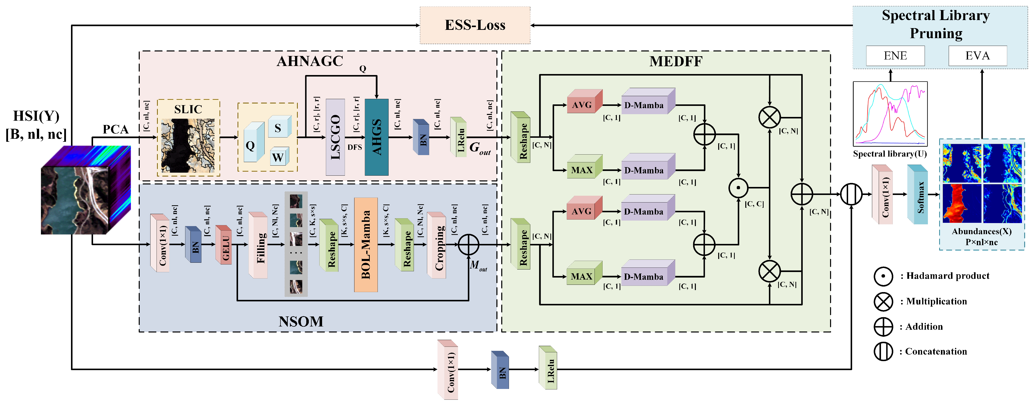
Next, we provide a detailed description of the DGMNet method in this chapter, and the overall architecture of this network is illustrated in Figure 2.

Specifically, the input HSI is first divided into global and local parallel branches to comprehensively capture its spatial information. The AHNAGC module extracts global spatial features through an adaptive hopping-neighborhood-aware graph convolution mechanism, while the NSOM focuses on accurately modeling the fine-grained local spatial structure. Subsequently, the MEDFF module leverages a spectral attention mechanism to enhance the spectral feature learning and effectively fuse the global and local spatial features, thereby strengthening the interaction and representation of spatial–spectral information. The fused features are subsequently concatenated with four dimension-reduced channels derived from the original HSI, and then projected into the abundance matrix through a 1D convolution followed by a softmax layer. This process is optimized under the guidance of a carefully designed loss function. Notably, during the model iteration, we introduce a spectral-library-pruning mechanism based on a sparse NN, which dynamically selects spectral features. This strategy significantly reduces redundant computation while maintaining the accuracy and robustness of the unmixing performance.

3.1. Adaptive Hop-Neighborhood-Aware GCN (AHNAGC)

To effectively extract global spatial features, we designed the AHNAGC module, which consists of two components: LSCGO and an AHGS.

After constructing the superpixel graph, the original GCN propagates information across all connected superpixels; however, some connections are based solely on spatial adjacency and may not reflect the true land-cover relationships. Such indiscriminate feature propagation can cause confusion between different land-cover classes, negatively affecting the HU accuracy. To mitigate this, the proposed LSCGO module enhances the regional spectral representation by averaging the local neighborhood. It then refines adjacency by removing connections with large spectral differences, allowing the model to focus on spectrally similar regions and improving the unmixing stability and accuracy.

Multi-hop graph structures have been widely used in HSI classification and unmixing [47,50], but they typically rely on preset hop numbers. This not only increases the feature engineering workload but also limits the generalization, as suboptimal hop settings may lead to information loss or redundancy, degrading the performance. To overcome this, we propose the AHGS module, which adaptively selects hop counts during each iteration without fixed manual settings. This dynamic mechanism captures global information more effectively, enhances the model expressiveness, and reduces the tuning effort.

Traditional convolution operations treat each pixel in the HSI as a node, resulting in an excessive number of nodes and greatly increasing the computational complexity of the adjacency matrix. Therefore, DGMNet employs the SLIC algorithm for superpixel segmentation, effectively reducing the number of nodes and generating three matrices: the transformation matrix between the pixels and superpixels $\mathit{Q}\in R^{N\times r}$, the superpixel adjacency matrix $\mathit{W}\in R^{r\times r}$, and the superpixel feature matrix $\mathit{S}\in R^{r\times C}$, where N denotes the number of pixels with $N=nl\times nc$, r is the number of superpixels, and C represents the number of channels after a dimensionality reduction.

$$\begin{array}{c}\mathit{Q}\left(i,j\right)=\left\{\begin{array}{cc}1,\hfill & if\widetilde{{\mathit{Y}}_i}\in \eta \left(r_j\right)\hfill \\ 0,\hfill & if\widetilde{{\mathit{Y}}_i}\notin \eta \left(r_j\right)\hfill \end{array}\widetilde{{\mathit{Y}}_i}=Flatten\left({\mathit{Y}}_{pca}\right)\right.\hfill \end{array}$$

(9)

$$\mathit{W}\left(i,j\right)=\left\{\begin{array}{cc}1,& if{r}_{i}and{r}_{j}areadjacent\left(i\ne j\right)\\ 0,& otherwise\end{array}\right.$$

(10)

where ${\mathit{Y}}_{pca}$ represents the dimensionality-reduced HSI, $Flatten$(·) refers to the process of flattening the ${\mathit{Y}}_{pca}$ along its spatial dimensions, and $\widetilde{{\mathit{Y}}_i}$ represents the i-th pixel of the flattened matrix. $\eta \left(r_j\right)$ represents the set of elements for the j-th superpixel, and $\mathit{W}\left(i,j\right)$ represents the value at the coordinates ($r_i$,$r_j$) in the adjacency relationship matrix.

(1) LSCGO: In this module, we optimize the correlation graph between superpixels through the constructed matrices W and S to better enhance the local spatial correlations.

First, the adjacency matrix $\mathit{W}$ and the identity matrix $\mathit{I}$ are added. Then, a dot-product operation is performed with $\mathit{S}$. That is, each row of $\mathit{W}$ is multiplied element-wise with the first dimension of $\mathit{S}$ to obtain $\mathit{W}\mathbf{1}=\left(\mathit{W}+\mathit{I}\right)\odot \mathit{S}$, where $\mathit{W}\mathbf{1}\in R^{r\times r\times C}$ and ⊙ denotes element-wise multiplication. Next, $\mathit{W}$ is again added to the identity matrix $\mathit{I}$, and then multiplied with $\mathit{S}$ to compute the average feature values over the neighborhood of each superpixel, i.e., $\mathit{W}\mathbf{2}=\left(\mathit{W}+\mathit{I}\right)\mathit{S}$, where $\mathit{W}\mathbf{2}\in R^{r\times C}$. Subsequently, the number of neighbors for the i-th superpixel, including itself, is computed as ${\xi }_i={∥{\mathit{W}}_{i,:}+{\mathit{I}}_{i,:}∥}_0$, where ${∥·∥}_0$ denotes the $l_0$-norm, which is used to count the number of non-zero elements in a row. Finally, $\mathit{W}\mathbf{2}$ is divided by $\xi$ to obtain the normalized matrix $\mathit{W}\mathbf{3}\in R^{r\times C}$, as shown in Equation (11):

$$\mathit{W}\mathbf{3}=\mathit{W}\mathbf{2}/\xi$$

(11)

where each element in $\mathit{W}\mathbf{3}$ reflects the mean feature value within the neighborhood region of a superpixel and is used to represent the overall characteristics of the neighborhood.

Subsequently, each row of $\mathit{W}\mathbf{1}$ is subtracted from the corresponding non-zero elements in $\mathit{W}\mathbf{3}$, with the self-relations of each superpixel removed. The resulting tensor, denoted as $\mathit{W}\mathbf{4}\in R^{r\times r\times C}$, reflects the strength of correlation between each pixel and its neighborhood in each dimension. The greater the correlation, the smaller the value in $\mathit{W}\mathbf{4}$. The detailed formulation is illustrated in Equation (12):

$$\mathit{W}{\mathbf{4}}_{i,j,C}=\left\{\begin{array}{cc}\mathit{W}{\mathbf{1}}_{i,j,C}-\mathit{W}{\mathbf{3}}_{j,C}\hfill & if\mathit{W}{\mathbf{1}}_{i,j,C}\ne 0\\ 0\hfill & otherwise\hfill \end{array}\right.$$

(12)

where $\mathit{W}{\mathbf{4}}_{i,i,:}=0$. Next, a channel-wise mean operation is performed on $\mathit{W}\mathbf{4}$ to obtain $\mathit{W}\mathbf{5}$, as shown in Equation (13).

$$\mathit{W}{\mathbf{5}}_{i,j}={\displaystyle \frac{1}{C}}\sum _{n=1}^C\mathit{W}{\mathbf{4}}_{i,j,n}$$

(13)

Then, we introduce a soft thresholding strategy. Based on the distribution of values in $\mathit{W}\mathbf{5}$, a random threshold parameter $\alpha$ was designed within the range $(0.4,1)$. By iterating through $\mathit{W}\mathbf{5}$ element-wise, values greater than $\alpha$ are set to 0, while those smaller than $\alpha$ are set to 1. As a result, a locally enhanced adjacency matrix ${\mathit{W}}^{\mathit{adj}}$ is obtained, as shown in Equation (14). This matrix disconnects neighboring superpixels that deviate significantly from the overall feature level of each local region, thereby enhancing the local spatial correlation.

$${\mathit{W}}_{i,j}^{\mathit{adj}}=\left\{\begin{array}{cc}1,\hfill & if\mathit{W}{\mathbf{5}}_{i,j}\le \alpha \hfill \\ 0,\hfill & if\mathit{W}{\mathbf{5}}_{i,j}>\alpha \hfill \end{array}\right.\forall i,j,\alpha \sim \mathcal{U}(0.4,1)$$

(14)

Finally, the average feature representation of each superpixel, denoted as ${\mathit{S}}^{\mathit{avg}}$, is computed, as shown in Equation (15), and the weight relationships between the superpixel nodes for non-zero elements in ${\mathit{W}}^{\mathit{adj}}$ is calculated using a Gaussian kernel function. The resulting weighted adjacency matrix is denoted as ${\mathit{W}}^{\mathit{lscgo}}$, as illustrated in Equation (16), where $\epsilon$ is a tunable hyperparameter.

$${\mathit{S}}_i^{\mathit{avg}}={\displaystyle \frac{1}{C}}\sum _{j=1}^C{\mathit{S}}_{ij},i=1,\dots ,r$$

(15)

$${\mathit{W}}_{i,j}^{\mathit{lscgo}}=\left\{\begin{array}{cc}exp\left(-{\displaystyle \frac{{\left({\mathit{S}}_i^{\mathit{avg}}-{\mathit{S}}_j^{\mathit{avg}}\right)}^2}{{\epsilon }^2}}\right)\hfill & if{\mathit{W}}_{i,j}^{\mathit{adj}}\ne 0\\ 0\hfill & otherwise\hfill \end{array}\right.$$

(16)

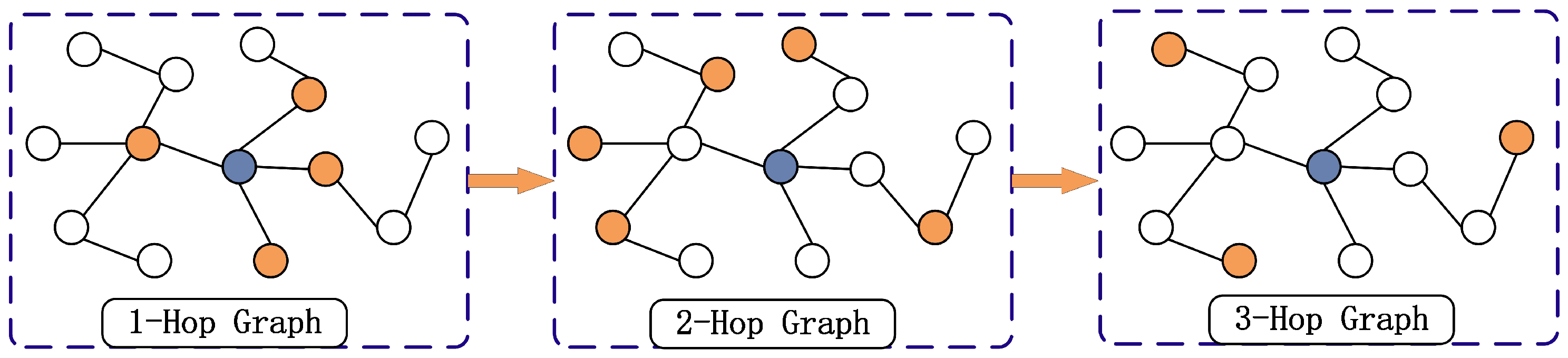
(2) The AHGS: In this module, a multi-hop graph structure is created based on ${\mathit{W}}^{\mathit{lscgo}}$, enabling adaptive selection and weighting of multi-hop features. The AHGS module is shown in Figure 3.

First, the adjacency weight matrix of the first-order multi-hop graph is defined as ${\mathit{A}}_1={\mathit{W}}^{\mathit{lscgo}}$. DFS is applied to each superpixel node to identify and record all the paths that are z hops away from the selected central node. The endpoints of these paths are then marked as $r_z$. Accordingly, the adjacency matrix of the z-th hop can be defined as

$${\mathit{A}}_z\left(r,r_z\right)={\displaystyle \frac{1}{z}}\left({\mathit{W}}_{(r,r_1)}^{\mathit{lscgo}}+{\mathit{W}}_{(r_1,r_2)}^{\mathit{lscgo}}+\dots \right.\left.+{\mathit{W}}_{(r_{z-1},r_z)}^{\mathit{lscgo}}\right)$$

(17)

where $r_1,r_2,...,r_z$ represents the intermediate nodes along the path. Therefore, the z-hop adjacency feature matrix is obtained by summing and averaging the $z-1$ adjacency feature matrices, which encompasses all the features of paths that range from 1 hop to z hops. Based on this method, a series of z-hop graph adjacency matrices can be generated, denoted as ${\mathit{A}}_1,{\mathit{A}}_2,...,{\mathit{A}}_z$. These matrices form the foundation of the multi-hop graph structure. In this structure, the direct neighbors of a central superpixel node are considered the 1-hop graph, the neighbors of neighbors form the 2-hop graph, and so on. This effectively avoids redundancy, expands the receptive field of a single node, and allows it to connect to more distant nodes via multi-hop propagation, thereby enhancing the network’s global perception capability. The results after applying graph convolution to the 1-hop, 2-hop, and z-hop adjacency feature matrices are as follows:

$$\begin{array}{cc}\hfill {\mathit{G}}_1& =BN\left(GCNB\left(BN\left(\mathit{S}\right),{\mathit{A}}_1\right)\right)\hfill \\ \hfill {\mathit{G}}_2& =BN\left(GCNB\left({\mathit{G}}_1,{\mathit{A}}_2\right)\right)\hfill \\ \hfill & ⋮\hfill \\ \hfill {\mathit{G}}_z& =BN\left(GCNB\left({\mathit{G}}_{z-1},{\mathit{A}}_z\right)\right)\hfill \end{array}$$

(18)

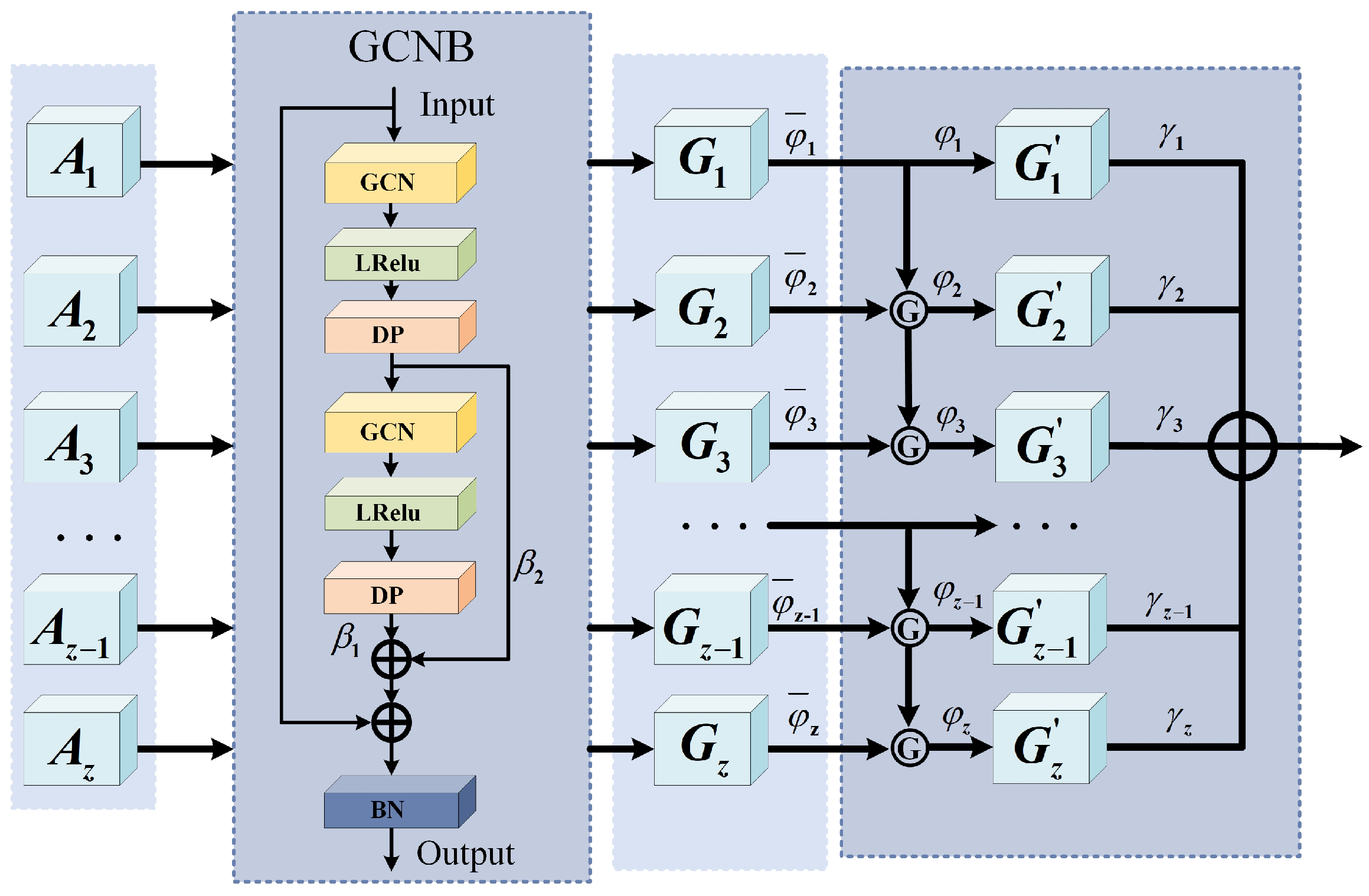
where ${\mathit{G}}_i\left(i=1,2,...,z\right)$ denotes the feature matrix obtained after the i-hop graph convolution, and $BN$ represents batch normalization. $GCNB$ is a carefully designed dual-layer graph convolution feature extraction module, which innovatively employs two cascaded graph convolution layers to achieve multi-level feature learning. A key advantage of this module lies in the introduction of a learnable dynamic weight matrix, which enables the model to adaptively balance the contribution of different feature levels through ${\beta }_i$. Meanwhile, a skip connection mechanism is incorporated to deeply fuse the original input features. This design not only preserves hierarchical information but also significantly enhances the model’s representational power and training stability, thereby delivering superior feature extraction performance when dealing with complex graph-structured data.

Next, two sets of learnable parameters are initialized, denoted as $\overline{\phi },\gamma \in R^z$, representing the hop selection factors and feature contribution factors, respectively. Meanwhile, a parameter matrix $\phi$ is initialized with the same dimensions as $\overline{\phi }$ to control the hop activation. During training, for each element in $\phi$, we introduced a fixed threshold (set to 0.3) to determine whether the corresponding hop feature is activated. Specifically, the hop control parameter matrix $\phi$ is computed as follows:

$${\phi }_i=\left\{\begin{array}{cc}1,\hfill & i=1\hfill \\ \left[\delta \left({\overline{\phi }}_i\right)>0.3\right]·{\displaystyle \prod _{j=1}^{i-1}}{\phi }_j,\hfill & i=2,3,,,z\hfill \end{array}\right.$$

(19)

where $\delta$ denotes the sigmoid activation function, $\left[·\right]$ represents the logical operator that returns 1 if the condition inside the brackets is true and 0 otherwise, and ∏ denotes the product operation. The above design enforces that the first-hop feature is always activated, while the activation of subsequent hops depends on whether all previous hops have been selected. Specifically, the z-th hop can only be activated if all preceding $1\sim z-1$ hops are also activated, ensuring the continuity of the feature selection. This operation is indicated by Ⓖ in Figure 3. Accordingly, the global spatial feature extracted by the AHGS module can be formulated as Equation (20):

$${\mathit{G}}_{AHGS}=\sum _{i=1}^z\mathrm{softmax}\left({\gamma }_i\right){\phi }_i{\mathit{G}}_i$$

(20)

To obtain the final pixel-level global spatial feature matrix ${\mathit{G}}_{out}\in R^{C\times nl\times nc}$ for subsequent feature fusion, the fused global spatial features are first projected back to the pixel domain via the pixel transformation matrix $\mathit{Q}$, and then refined through $BN$ and LeakyReLU ($LReLU$), as defined in Equation (21):

$${\mathit{G}}_{out}=LReLU\left(BN\left(\mathit{Q}{\mathit{G}}_{AHGS}\right)\right)$$

(21)

3.2. Neighborhood Spatial Offset Mamba (NSOM)

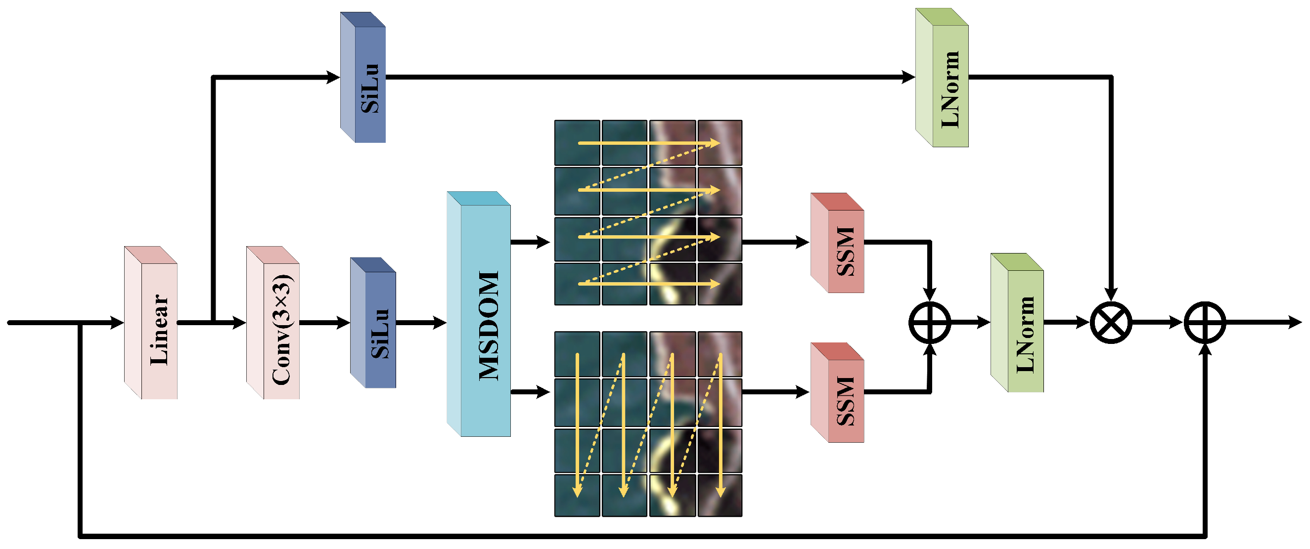
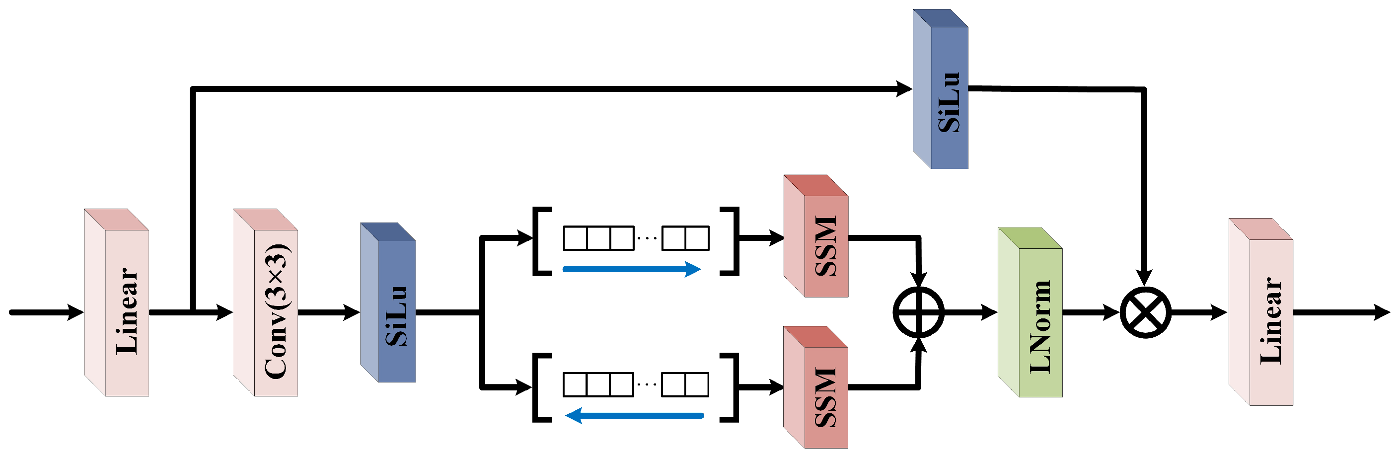
In HU tasks, the fine spectral information of local spatial features plays a crucial role in accurately analyzing the composition of mixed pixels. To enhance the model’s capability for modeling local spatial structures and to collaboratively extract multi-level spatial information with the AHNAGC module, we designed the NSOM module. Within this module, we propose BOL-Mamba, as illustrated in Figure 4. BOL-Mamba integrates MSDOM (shown in Figure 5) with a bidirectional Mamba architecture, enabling the fine-grained characterization and modeling of spatial information.

The MSDOM module employs multi-scale deformable convolutions for dynamic sampling, overcoming the limitations of fixed receptive fields and enabling the adaptive capture of fine textures and multi-scale spatial patterns. To overcome the global perception limitations of MSDOM, a bidirectional Mamba is introduced to model long-range dependencies along horizontal and vertical directions within HSI blocks. Leveraging Mamba’s efficient sequence modeling, this design enhances the intra-block spatial perception and global context modeling. The synergy between MSDOM and bidirectional Mamba enables comprehensive and structured spatial feature extraction. Meanwhile, its lightweight design ensures a low computational and parameter overhead, providing a robust foundation for downstream tasks.

The input HSI $\mathit{Y}\in R^{B\times \mathrm{nl}\times nc}$ is first passed through a $1\times 1$ convolution to reduce its dimensionality to C channels, followed by normalization and activation. To ensure that the spatial dimensions of the feature map can be evenly divided into K fixed-size blocks, reflection padding is applied along the height and width dimensions. This padding strategy not only ensures tidy block partitioning but also mitigates modeling bias caused by edge effects. Finally, the padded feature map is reshaped into non-overlapping blocks. The process can be formally described as

$${\mathit{M}}_1=\mathrm{Reshape}\left(\mathrm{Filling}\left(GELU\left(BN\left(Con{v}_{1\times 1}\left(\mathit{Y}\right)\right)\right)\right)\right)$$

(22)

where $\mathrm{Filling}$ and $GELU$ represent the reflection padding operation and the activation function, respectively. ${\mathit{M}}_1\in R^{K\times {\mathrm{s}}^2\times C}$ denotes the resulting 3D feature tensor. $Nl$ and $Nc$ represent the height and width of the image after padding, respectively. s denotes the width of each HSI block, and ${\mathrm{s}}^2=\left(Nl\times Nc\right)/K$.

${\mathit{M}}_1$ is subsequently fed into the BOL-Mamba module for further feature learning. Within BOL-Mamba, the channel dimension of ${\mathit{M}}_1$ is first expanded to twice its original size through a linear transformation, and then evenly split into two feature sub-tensors, denoted as ${\mathit{M}}_{21}\in R^{K\times {\mathrm{s}}^2\times C}$ and ${\mathit{M}}_{22}\in R^{K\times {\mathrm{s}}^2\times C}$. To enhance the representation capability of the local spatial context, we introduce a $3\times 3$ convolution operation after the linear mapping, and after passing through the activation function, the result is fed into our designed MSDOM module. The formula is shown as follows:

$${\mathit{M}}_3=\mathrm{MSDOM}\left(\mathrm{SiLu}\left(\mathrm{Con}{\mathrm{v}}_{3\times 3}\left({\mathit{M}}_{21}\right)\right)\right)$$

(23)

where ${\mathit{M}}_3\in R^{K\times C\times s^2}$ represents the resulting feature map. MSDOM first extracts local information under different receptive fields through parallel single-layer convolutions with $3\times 3$, $5\times 5$, and $7\times 7$ kernels, and combines a learnable offset strategy to achieve dynamic adaptation to the local spatial structure.

To enhance the capability of sequential modeling along different spatial dimensions, ${\mathit{M}}_3\in R^{K\times C\times {\mathrm{s}}^2}$ is input into the SSM module through two parallel paths: the original form and a variant with height and width swapped. This allows the model to capture long-range dependencies along different spatial directions, improving the completeness of the spatial context modeling. After processing, the output of the variant path is restored to the original dimensions and summed with the output of the original path, achieving effective bidirectional spatial feature fusion. The specific formulation is as follows:

$${\mathit{M}}_4=\mathrm{SSM}\left({\mathit{M}}_3\right)+\mathrm{Reshape}\left(\mathrm{SSM}\left(\mathrm{Reshape}\left({\mathit{M}}_3\right)\right)\right)$$

(24)

Furthermore, ${\mathit{M}}_4$ is first normalized and then element-wise multiplied with ${\mathit{M}}_{22}$, which has been processed by activation and normalization. This facilitates feature refinement guided by attention signals. To preserve the original feature information and avoid potential information loss, a residual connection is employed. The above process can be formulated as follows:

$${\mathit{M}}_6=LNorm\left(\mathrm{SiLu}\left({\mathit{M}}_{22}\right)\right)\odot LNorm\left({\mathit{M}}_4\right)+{\mathit{M}}_1$$

(25)

where ⊙ denotes element-wise multiplication. This mechanism not only enhances the model’s ability to extract key features but also improves the training stability and feature robustness of the deep network structure. Finally, to ensure that the output features maintain the same spatial dimensions as the original input, spatial dimension restoration is performed by removing the previously added padding. The resulting features are then fused with shallow features to produce the final output features ${\mathit{M}}_{out}\in R^{C\times \mathrm{nl}\times nc}$, which can be formulated as

$${\mathit{M}}_{out}=\mathrm{Cropping}\left({\mathit{M}}_6\right)+GELU\left(BN\left(Con{v}_{1\times 1}\left(\mathit{Y}\right)\right)\right)$$

(26)

In summary, the NSOM module enhances the spatial discriminative capability and adaptability of the model in HU tasks by integrating Mamba with low computational complexity, thereby enabling dynamic perception, multi-scale fusion, and sequential modeling of local spatial features.

3.3. Mamba-Enhanced Dual-Stream Feature Fusion (MEDFF)

To further enhance the model’s ability to capture complex image features, we propose the MEDFF module. This module significantly improves the model performance by fusing global and local spatial features and integrating a spectral attention mechanism, along with a residual structure. The spectral attention mechanism adaptively adjusts the weights of the individual spectral channels, enabling the model to focus on critical information and enhancing its sensitivity to important features. The introduction of the residual structure ensures effective information flow across different layers of the network, which mitigates the vanishing gradient problem and improves the model stability. Through this combination of designs, MEDFF not only enhances the feature representation capability but also improves the model’s robustness and generalization ability.

First, the global spatial features ${\mathit{G}}_{out}\in R^{C\times nl\times nc}$ and local spatial features ${\mathit{M}}_{out}\in R^{C\times nl\times nc}$ are processed using average pooling and max pooling, respectively, to extract the overall information along the channel dimension and capture the most salient features. The specific computation is as follows:

$$f_{G11}=AVG\left({\mathit{G}}_{out}\right),f_{G12}=MAX\left({\mathit{G}}_{out}\right)$$

(27)

$$f_{M11}=AVG\left({\mathit{M}}_{out}\right),f_{M12}=MAX\left({\mathit{M}}_{out}\right)$$

(28)

Through pooling operations, the features of each channel are compressed into a single value, forming a serialized feature representation. To efficiently learn these sequential features, we leveraged the advantages of the Mamba model and designed a D-Mamba module, as shown in Figure 6. This module performs bidirectional sequence learning in both forward and backward directions, enabling it to simultaneously capture complex dependencies between channels and promote feature interaction and fusion. The specific computation process is as follows:

$$f_{G21}=\mathrm{D}\text{-}\mathrm{Mamba}\left(f_{G11}\right),f_{G22}=\mathrm{D}\text{-}\mathrm{Mamba}\left(f_{G12}\right)$$

(29)

$$f_{M21}=\mathrm{D}\text{-}\mathrm{Mamba}\left(f_{M11}\right),f_{M22}=\mathrm{D}\text{-}\mathrm{Mamba}\left(f_{M12}\right)$$

(30)

Subsequently, the features processed by D-Mamba are fused effectively by performing element-wise addition and multiplication operations:

$$f_3=\left(f_{G21}+f_{G22}\right)\odot \left(f_{M21}+f_{M22}\right)$$

(31)

Finally, the spectral attention mechanism adds $f_3$ to the original HSI, and then concatenates it with partial spectral features ${\mathit{Y}}^{\prime }\in R^{B^{\prime }\times nl\times nc}$ from the original HSI to obtain the final feature map ${\mathit{F}}_{out}\in R^{\left(C+B^{\prime }\right)\times nl\times nc}$. The specific formula is as follows:

$${\mathit{F}}_{out}=\mathrm{Concat}\left(\left(f_3{\mathit{G}}_{out}+{\mathit{G}}_{out}+f_3{\mathit{M}}_{out}+{\mathit{M}}_{out}\right),{\mathit{Y}}^{\prime }\right)$$

(32)

3.4. Spectral Library Pruning

We innovatively integrated a spectral-library-pruning strategy into NN unmixing models. This innovative design effectively addresses the high coherence and large-scale drawbacks commonly encountered in traditional unmixing methods [16], while significantly reducing the model’s parameter count and computational complexity. The implementation of this strategy can be divided into two key steps: endmember number estimation (ENE) and endmember validity assessment (EVA).

(1) ENE: Singular value decomposition (SVD) can decompose a matrix into orthogonal bases with clear statistical meaning, where the magnitude of singular values reflects the importance of each component. Therefore, this paper uses SVD to determine the number of endmembers to retain. Specifically, P singular values are computed via SVD, then a threshold $\tau$ is set, and the number of singular values exceeding this threshold is taken as the final number of retained endmembers. The calculation formula is as follows:

$$P^{\prime }=\sum _{i=1}^P\left[{\sigma }_i>\tau \right]$$

(33)

where $\sigma$ denotes the singular values. The effectiveness of this method is further discussed in the Section 5.

(2) EVA: During the unmixing process, the abundances matrix is typically sparse, with most row vectors approaching zero and only a few containing significant non-zero elements. These non-zero rows correspond to endmember components that are actually present in the HSI, while the near-zero rows represent dictionary atoms that contribute little to the unmixing process. To quantify the activity level of each endmember, the $l_1$ norm is applied to each row of the abundances matrix for the activity assessment, and then min–max normalization is performed to obtain standardized activity indicators, as shown in Equation (35). The min–max normalization (MNorm) is defined in Equation (34):

$$\mathrm{MNorm}\left({\mathit{X}}_i\right)={\displaystyle \frac{{\mathit{X}}_i-min\left(\mathit{X}\right)}{max\left(\mathit{X}\right)-min\left(\mathit{X}\right)}}$$

(34)

$$\begin{array}{cc}{\mathit{SA}}_i=\mathrm{MNorm}\left({\mathit{X}}_{i1}\right)& =\mathrm{MNorm}\left({\displaystyle \sum _{j=1}^{nl\times nc}}\left|{\mathit{X}}_{ij}\right|\right),fori=1,2,\dots ,P\end{array}$$

(35)

In addition, inspired by [51], we propose a new effectiveness evaluation strategy from the perspective of energy, aiming to prevent small-target endmembers from being pruned during the iterative process. Specifically, the contribution of each endmember to the reconstructed image is calculated, and can be reflected by the difference between the original image and the reconstructed image obtained after removing the corresponding endmember. The larger the difference, the greater the contribution of that endmember. Subsequently, the contribution values are normalized, as formulated below:

$${\mathit{U}}^{(-i)}=\mathit{U}[:,-i],{\mathit{X}}^{(-i)}=Flatten\left(\mathit{X}[-i,:]\right)$$

(36)

$${\mathit{Y}}^{(-i)}={\mathit{U}}^{(-i)}{\mathit{X}}^{(-i)}$$

(37)

$${\mathit{Cn}}_i=\mathrm{MNorm}\left({∥{\mathit{Y}}^{(-i)}-Flatten\left(\mathit{Y}\right)∥}_F\right)$$

(38)

where ${\mathit{U}}^{(-i)}$ denotes the matrix $\mathit{U}$ with its i-th column removed. Next, the maximum value of each row in the abundances matrix (i.e., the energy) is computed and multiplied with the corresponding contribution value, which serves as a new evaluation criterion, as defined in Equation (39):

$${\mathit{IEC}}_i=\mathrm{MNorm}\left({max}_j\left({\mathit{X}}_{i,j}\right){\mathit{Cn}}_i\right)$$

(39)

The final evaluation strategy is as follows:

$${\mathit{Criteria}}_i={\mathit{SA}}_i+{\mathit{IEC}}_i$$

(40)

This evaluation strategy effectively addresses the issues of high spectral library coherence and large-scale complexity by jointly considering the atom activity, correlation, and a small-target preservation mechanism. At the same time, it significantly reduces the model’s parameter count.

(3) Pruning process: Specifically, during the first stage of iteration ($Loop\_iter=Iter1$), the need for feature dimension reduction is dynamically determined based on the SVD singular value analysis results. If $P/4>P^{\prime }$, the first $P/4$ principal columns and rows of $\mathit{U}$ and $\mathit{X}$ are retained, namely, $\mathit{U}\in R^{B\times \left(p/4\right)}$ and $\mathit{X}\in R^{\left(p/4\right)\times N}$. Otherwise, the process enters the second stage ($Loop\_iter=Iter2$) to retain P key features.

3.5. Enhanced Sparsity Smoothing Loss (ESS-Loss)

This paper proposes the ESS-Loss, which significantly improves the model performance by combining the reconstruction error with multiple prior conditions of the HSI. To measure the reconstruction quality, the mean squared error (MSE) is adopted as the loss function. The MSE is a widely used metric in regression tasks that aims to minimize the difference between the reconstructed image and the original image. Its formula is as follows, where ${\mathit{Y}}_i$ and ${\widehat{\mathit{Y}}}_i$ represent the spectral vectors of the original and estimated images, respectively:

$${\mathcal{L}}_{MSE}={\displaystyle \frac{1}{N}}\sum _{i=1}^N{\left({\mathit{Y}}_i-{\widehat{\mathit{Y}}}_i\right)}^2$$

(41)

Based on the sparsity prior of the abundances matrix, [13] proposed an $l_{1/2}$ sparse-constrained NMF, which enhances the abundances sparsity through an $l_{1/2}$ regularization term. They demonstrated that the $l_{1/2}$ regularizer is easier to optimize than the $l_0$ regularizer and achieves stronger sparsity than the $l_1$ regularizer. Therefore, this paper adopts the $l_{1/2}$ norm as the sparsity loss, formulated as follows:

$${\mathcal{L}}_{1/2}={\lambda }_{1/2}{∥\mathit{X}∥}_{1/2}={\lambda }_{1/2}\sum _{i=1}^P\sum _{j=1}^N{\left|{\mathit{X}}_{ij}\right|}^{1/2}$$

(42)

To impose smoothness constraints on the abundances, this paper extends the traditional TV loss by introducing diagonal directions and incorporating a pixel-wise local gradient-based adaptive weighting mechanism. Traditional TV loss typically considers only pixel differences in the horizontal and vertical directions, overlooking diagonal structures within the image. To enhance the model’s ability to perceive structural information, we propose enhanced total variation (ETV). This loss calculates pixel gradient differences in four directions: horizontal, vertical, diagonal, and anti-diagonal. The pixel gradient differences in these four directions are defined as follows:

$$\begin{array}{cccc}\hfill {\mathrm{grad}}_h& ={\mathit{X}}_{i+1,j}-{\mathit{X}}_{i,j},\hfill & \hfill {\mathrm{grad}}_v& ={\mathit{X}}_{i,j+1}-{\mathit{X}}_{i,j}\hfill \\ \hfill {\mathrm{grad}}_{d1}& ={\mathit{X}}_{i+1,j+1}-{\mathit{X}}_{i,j},\hfill & \hfill {\mathrm{grad}}_{d2}& ={\mathit{X}}_{i+1,j-1}-{\mathit{X}}_{i,j}\hfill \end{array}$$

(43)

Based on the gradient information in the four directions mentioned above, the average gradient magnitude of each pixel is defined as follows:

$$\mathrm{grad}={\displaystyle \frac{1}{4}}\left(|\mathrm{gra}{\mathrm{d}}_h|+|\mathrm{gra}{\mathrm{d}}_v|+|\mathrm{gra}{\mathrm{d}}_{d1}|+|\mathrm{gra}{\mathrm{d}}_{d2}|\right)$$

(44)

This gradient value is used to construct the pixel-level adaptive weight matrix $\mathit{w}$, which is defined as follows:

$$\mathit{w}=exp\left(-{\displaystyle \frac{\mathrm{gra}{\mathrm{d}}^2}{2{\mu }^2}}\right)$$

(45)

where the parameter $\mu$ controls the width of the Gaussian function. This adaptive weighting mechanism assigns weights to each pixel based on the local gradient: regions with large gradients are assigned smaller weights to avoid the excessive smoothing of image edges, while flat regions are given larger weights to enhance the smoothness. Through this dynamic adjustment, the loss function can be flexibly optimized according to pixel values, preserving important edge structures while suppressing unnecessary noise.

Considering the contribution of different directions to the image structure, we divided the loss into two parts: the horizontal and vertical direction loss $ET{V}_{hv}$, and the diagonal direction loss $ET{V}_{diag}$:

$$ET{V}_{hv}={\displaystyle \frac{1}{N}}\sum _{i,j}{\mathit{w}}_{i,j}\left[{\left({\mathit{X}}_{i+1,j}-{\mathit{X}}_{i,j}\right)}^2+{\left({\mathit{X}}_{i,j+1}-{\mathit{X}}_{i,j}\right)}^2\right]$$

(46)

$$ET{V}_{diag}={\displaystyle \frac{1}{N}}\sum _{i,j}{\mathit{w}}_{i,j}\left[{({\mathit{X}}_{i+1,j+1}-{\mathit{X}}_{i,j})}^2+{({\mathit{X}}_{i+1,j-1}-{\mathit{X}}_{i,j})}^2\right]$$

(47)

The final ETV loss function is defined as follows:

$${\mathcal{L}}_{ETV}={\lambda }_{hv}·ET{V}_{hv}+{\lambda }_{diag}·ET{V}_{diag}$$

(48)

where ${\lambda }_{hv}$ and ${\lambda }_{diag}$ are hyperparameters that control the balance between the two directions. The final loss can be expressed as

$$ESS\text{-}Loss={\mathcal{L}}_{MSE}+{\mathcal{L}}_{1/2}+{\mathcal{L}}_{ETV}$$

(49)

4. Experimental Results and Analysis

The performance of the proposed method is evaluated in this section. Two synthetic and five real datasets were selected for the algorithm experiments, and a comparative analysis with nine state-of-the-art methods was performed to verify the effectiveness. The evaluation of each synthetic dataset was performed at three additive signal-to-noise ratios (SNRs), where the SNR is defined as $SN{R}_{dB}=10{log}_{10}E\left[y^{\top }y\right]/E\left[g^{\top }g\right]$, where y and g are the observed value and noise of the pixel, respectively, and $E[·]$ denotes the expectation operator; the tested SNRs were 20 dB, 30 dB, and 40 dB. The nine algorithms comprised six sparse unmixing algorithms based on representation models (SUnSAL (https://github.com/Laadr/SUNSAL (accessed on 1 May 2025))) [15], SUNSAL-TV (https://github.com/jinju123/RSSUn_TV (accessed on 1 May 2025)) [27], S2WSU (https://github.com/ricardoborsoi/MUA_SparseUnmixing (accessed on 1 May 2025)) [26], MUA (https://github.com/ricardoborsoi/MUA_SparseUnmixing (accessed on 1 May 2025)) [28], LSU (https://github.com/XiangfeiShen (accessed on 1 May 2025)) [16], and FaSUn (https://github.com/BehnoodRasti/FUnmix (accessed on 1 May 2025)) [32]) and three NN algorithms (SUnCNN (https://github.com/BehnoodRasti/SUnCNN (accessed on 1 May 2025)) [21], SVATN (https://github.com/MeiShaohui/SVATN (accessed on 1 May 2025)) [45], and PMGMCN [47]). The experimental results are based on a maximum of twenty independent experiments, with optimal results shown in bold and suboptimal results underlined. Additionally, the contribution of the three submodules and their impacts on the overall performance were evaluated through ablation experiments.

4.1. Hyperspectral Datasets

The experiments in this study were conducted on two synthetic datasets and five real datasets. The endmember spectra curves and pseudo-color images for the synthetic datasets are illustrated in Figure 7. The real datasets include Jasper Ridge, Samson, Cuprite, Urban, and ShaHu, with their corresponding pseudo-color images shown in Figure 8.

Among them, the ShaHu dataset from Ningxia (38.6578°N, 104.08296°E) was acquired by the Gaofen-5 (GF-5) satellite. The original HSI underwent radiometric and geometric corrections, which resulted in 330 valid spectral bands with a spatial resolution of $101\times 101$ pixels. Based on the VCA algorithm, 200 candidate endmembers were initially extracted from the original HSI. Subsequently, the endmember selection was performed using a spectral angle threshold of $3.33$ radians, which ultimately yielded 34 of the most representative spectral atoms to construct the spectral library. For comparison, the reference abundance maps were generated using ENVI^® software (L3Harris Geospatial, Boulder, CO, USA).

4.2. Evaluation Metrics

In synthetic datasets, since the ground-truth abundances are known, the discrepancy between the estimated and true abundances is quantified using the signal reconstruction error (SRE). A higher SRE value indicates a greater similarity between the original and estimated abundances. The formula is shown in Equation (50), where $\mathit{X}$ and ${\mathit{X}}^{\prime }$ represent the original and reconstructed abundance images, respectively:

$$\mathrm{SRE}\left(\mathit{X},{\mathit{X}}^{\prime }\right)=10{log}_{10}{\displaystyle \frac{{\parallel \mathit{X}\parallel }_F}{{∥\mathit{X}-{\mathit{X}}^{\prime }∥}_F}}$$

(50)

However, since the abundances of real HSIs are unknown beforehand, the root-mean-square error (RMSE) is used as the evaluation metric. A lower RMSE value indicates a higher similarity between the original HSI and the reconstructed HSI. The formula is shown in Equation (51):

$$\mathrm{RMSE}\left(\mathit{Y},{\mathit{Y}}^{\prime }\right)=\sqrt{{\displaystyle \frac{\parallel \mathit{Y}-{\mathit{Y}}^{\prime }{\parallel }_F^2}{LN}}}$$

(51)

where $\mathit{Y}$ and ${\mathit{Y}}^{\prime }$ represent the original and reconstructed HSI, respectively, while L and N denote the number of bands and the number of pixels, respectively.

4.3. Parameter Setting

The parameter settings for each comparison algorithm and the proposed algorithm are provided in

Table 1. Selection of parameters for each method.

Methods/Datasets	Synthetic Datasets	Real Datasets
SUnSAL [15]	$\lambda =0.01$	$\lambda =0.005$
SUnSAL_TV [27]	$\lambda =0.01,{\lambda }_{TV}=0.001,\mu =0.2$	$\lambda =0.01,{\lambda }_{TV}=0.0001,\mu =0.5$
S2WSU [26]	${\lambda }_{swsp}=0.0001,\mu =0.5$	${\lambda }_{swsp}=0.0005,\mu =0.5$
MUA_SLIC [28]	${\lambda }_1=0.01,{\lambda }_2=0.1,$	${\lambda }_1=0.01,{\lambda }_2=0.01,$
	$\beta =0.01,slic\_size=6,slic\_reg=0.005$	$\beta =10,slic\_size=200,slic\_reg=0.01$
LSU [16]	$\alpha =0.05,\beta =0.005,\mu =0.1$	$\alpha =0.05,\beta =5,\mu =0.1$
SUnCNN [21]	$Iter=2000$	$Iter=2000$
SVATN [45]	$Iter=2000$	$Iter=2000$
FaSUn [32]	$T=10000,T_A=T_B=5,{\mu }_1=50,{\mu }_2=2,{\mu }_3=1$	$T=10000,T_A=T_B=5,{\mu }_1=400,{\mu }_2=20,{\mu }_3=1$
PMGMCN [47]	$Iter=1500,r=255,Hop-counts=3,$	$Iter=1500,r=366,Hop-counts=3,\phi =0.002$
	$\phi =0.004\left(20\mathrm{dB}\right),\phi =0.0005\left(30\mathrm{dB}\right),\phi =0.0002\left(40\mathrm{dB}\right)$
Proposed	$Iter1=600,Iter2=1000,{\lambda }_{hv}=0.01,$	$Iter1=50,Iter2=1000,{\lambda }_{hv}=0.02,$
	${\lambda }_{diag}=0.002,{\lambda }_{1/2}=0.01,s=16,r=255$	${\lambda }_{diag}=0.005,{\lambda }_{1/2}=0.02,s=16,r=366$

. Additionally, the proposed method utilized the Adam optimizer with the learning rate set to $1\times {10}^{-3}$. Python $3.8.19$ was employed as the programming language for conducting the experiments, while PyTorch $1.10.1$ served as the programming environment, along with CUDA version $11.3$. The experiments were conducted on a computer equipped with an Intel^®(Santa Clara, CA, USA) Core™ i5-12600KF CPU, 32 GB of RAM, and an NVIDIA(Santa Clara, CA, USA) GeForce RTX™ 3060 (with 12 GB of GPU memory).

4.4. Experiments on Synthetic Datasets

(1) Parameter selection for ${\lambda }_{1/2}$: The choice of the sparsity parameter ${\lambda }_{1/2}$ plays a crucial role in the unmixing accuracy. As shown in the experimental analysis in Figure 9, when dd was set to 0.01 (red dot), the model achieved an optimal balance between the abundance sparsity and reconstruction error. Specifically, if the parameter is too small, it results in insufficient sparsity, generating many small but non-zero abundance values and thereby reducing the unmixing accuracy. Conversely, an excessively large value, while enhancing the sparsity, may suppress true endmember signals and lead to a lower SRE. Therefore, the sparsity parameter ${\lambda }_{1/2}$ was set to 0.01 to balance the sparsity and unmixing performance.

(2) Parameter selection for ${\mathcal{L}}_{ETV}$: The experimental results in Figure 10 demonstrate that when ${\lambda }_{hv}=0.01$ and ${\lambda }_{diag}$= 0.002, the model achieved an optimal balance between spatial smoothness constraints and detail preservation. From the perspective of the unmixing mechanism, a too-small parameter results in insufficient spatial regularization, leading to non-physical discontinuities in the abundances, whereas a too-large parameter causes over-smoothing, which obscures critical spatial details. This optimal combination not only significantly improves the accuracy of the abundance estimation but also ensures spatial continuity in the endmember distributions. Thus, on DC1 at 20 dB, ${\lambda }_{hv}$ and ${\lambda }_{diag}$ were set to 0.01 and 0.002, respectively, to balance the smoothness constraints in the horizontal, vertical, and diagonal directions.

(3) Parameter selection of patch size s²: Figure 11 demonstrates that the model achieved its optimal performance of $8.82$ when the patch size was set to 16 × 16, indicating that this size effectively balanced the spatial information capture and feature extraction accuracy for the given dataset. When the patch size was smaller than 16 × 16, insufficient local feature extraction led to a degraded performance; conversely, larger patch sizes introduced redundant information or caused boundary blurring, and thus, reduced the unmixing accuracy. It is important to note that the optimal patch size depends on the spatial characteristics of the dataset and the distribution of ground objects. Variations in spatial heterogeneity across different scenarios can significantly impact the applicability of patch partitioning strategies. Therefore, in practical applications, the patch size should be adaptively adjusted based on data characteristics to achieve an optimal balance between the unmixing accuracy and model robustness.

(4) The experiments with the DC1 synthetic dataset under different SNR levels:

Table 2. The SRE values of each algorithm on DC1 at three SNRs.

DC1	SUnSAL	SUnSAL-TV	S2WSU	MUA_SLIC	LSU	SUnCNN	SVATN	FaSUn	PMGMCN	Proposed
20 dB	6.3	6.9	6.86	5.78	6.51	5.76	6.92	5.76	7.99	8.82
30 dB	8.65	8.61	8.74	8.05	8.72	11.05	11.14	10.62	11.65	$\mathbf{12.16}$
40 dB	12.94	14.67	13.45	11.62	13.44	15.37	14.63	15.49	15.86	$\mathbf{16.23}$
Times (s)	$\mathbf{3.86}$	37.95	12.49	8.7	73.6	111.47	134.92	64.81	141.09	158.44

summarizes the unmixing performance of various methods on the DC1 dataset. It can be observed that DGMNet achieved the highest SRE under all SNR conditions, and thus, demonstrated superior robustness. Under low-SNR conditions, SVATN performed relatively well, which benefited from its variable dictionary mechanism that effectively mitigates noise interference. Figure 12 presents the abundance maps of each method at 20 dB, with GT representing the ground truth distribution. The comparison shows that SUnSAL and SUnSAL-TV produced large errors; SUnCNN and FaSUN were noticeably affected by noise, although their performance improved under a higher SNR. PMGMCN ranked next, as its receptive field modeling enhanced the spatial feature extraction. In contrast, DGMNet achieved the best unmixing results by precisely modeling the spectral spatial features through the integration of global GCN and local Mamba mechanisms.

(5) The experiments with the DC2 synthetic dataset under different SNR levels:

Table 3. The SRE values of each algorithm on DC2 at three SNRs.

DC2	SUnSAL	SUnSAL-TV	S2WSU	MUA_SLIC	LSU	SUnCNN	SVATN	FaSUn	PMGMCN	Proposed
20 dB	4.45	4.68	5.71	4.76	5.01	7.88	8.40	5.76	9.35	$\mathbf{9.64}$
30 dB	8.43	8.67	10.65	9.37	10.06	11.22	11.25	10.62	11.29	$\mathbf{12.5}$
40 dB	9.28	9.66	13.96	10.79	13.99	13.57	13.89	14.17	14.32	$\mathbf{14.44}$
Times (s)	$\mathbf{3.15}$	53.84	21.33	8.16	63.69	210.54	111.44	77.6	101.02	218.39

presents the performance comparison of various unmixing methods under different noise levels, highlighting the fundamental differences in their architectural designs. DGMNet consistently achieved the highest SRE across all the SNR conditions, which demonstrated its superior capability in spectral spatial joint modeling and adaptive feature fusion. In contrast, PMGMCN showed strong robustness under high noise conditions due to its use of a TV loss constructed with Sobel and Gaussian functions, which effectively mitigated noise interference. On the other hand, SVATN leveraged spectral variability modeling and convex constraints to exhibit greater stability in high-SNR scenarios. The visual results in Figure 13 further show that DGMNet provides the most accurate abundances estimates for most endmembers, which underscored its advantage in jointly modeling spatial and spectral information.

4.5. Experiments on Real Datasets

(1) Experiment on the influence of the atomic number of the spectral library: This experiment systematically analyzed the impact of the spectral library size on the computational efficiency of unmixing algorithms, based on the Urban dataset. As shown in Figure 14, the runtime of all methods increased with the number of spectral atoms, with SUnSAL demonstrating the highest computational efficiency. In contrast, methods such as SUnCNN, SVATN, and PMGMCN exhibited a greater sensitivity to the size of the spectral library, which led to a more noticeable increase in the runtime. The proposed method employs an adaptive spectral-library-pruning strategy to intelligently select representative endmembers and incorporates a dynamic dimensionality reduction. This not only ensures a high unmixing accuracy but also effectively reduces the sensitivity to the spectral library size, demonstrating strong potential for practical applications.

(2) Experiments on Jasper Ridge dataset: As shown in Figure 15, a comparison with the reference abundance maps revealed that although all the methods could roughly identify water regions, S2WSU, MUA, and LSU suffered from significant over-smoothing of the internal details, while FaSUn mistakenly classified some roads as water. In contrast, SUnCNN, PMGMCN, and the proposed method more accurately reconstructed the water structure, where the proposed method demonstrated clear advantages in estimating fine water-related details. For the road unmixing, S2WSU, MUA, and SUnCNN exhibited excessive smoothing, which resulted in partial road omission, whereas the abundance maps generated by SVATN and FaSUn contained many misclassifications. In comparison, the proposed method more precisely reconstructed the main road areas, which offered richer detail and sharper boundaries. Overall, the proposed method demonstrated stronger noise suppression and better spatial detail preservation on the Jasper Ridge dataset. The abundance maps generated by DGMNet exhibited a high contrast and clear structure, which validated the effectiveness of the proposed method in complex scenarios.

(3) Experiments on Samson dataset: As shown in Figure 16, a comparison with the reference abundance maps indicates that most algorithms could roughly reconstruct the soil distribution. However, SUnSAL, S2WSU, MUA, and LSU generally underestimated the abundance values. While SUnSAL-TV offered noise suppression capabilities, it produced over-smoothed abundance maps with blurred boundaries. In contrast, SUnCNN, SVATN, FaSUn, and the proposed method delivered better performance when estimating the soil and tree regions, as characterized by clear edges and accurate predictions. This is attributed to their stronger modeling capacity of complex spatial–spectral relationships. For the water estimation, LSU and FaSUn exhibited obvious misclassification in non-water areas. The proposed method, however, achieved the best performance in boundary identification and detail preservation of water regions by combining low noise levels with high spatial resolution. In summary, the proposed method demonstrated superior boundary delineation and noise suppression across all three land-cover types and outperformed the mainstream algorithms overall.

(4) Experiments on the Cuprite dataset: The abundance maps in Figure 17 indicate that although most methods could roughly reconstruct the distribution of alunite, SUnSAL, SUnCNN, and SVATN exhibited evident over-smoothing, which led to estimation failures in certain regions. For the estimation of andradite, SUnCNN, SVATN, PMGMCN, and the proposed method performed well, where they accurately identified mineral distributions while effectively suppressing noise, and thus, demonstrated the advantages of deep models in nonlinear feature modeling. In the estimation of chalcedony, the proposed method showed clear boundaries and rich details. Overall, the proposed method exhibited lower noise and stronger detail preservation when estimating various endmembers, such as andradite, buddingtonite, and montmorillonite. The resulting abundance maps were characterized by a high contrast and clarity, which fully showcased the superior unmixing performance of the proposed method.

(5) Experiments on the Urban dataset: The results in Figure 18 demonstrate that the deep learning methods, owing to their powerful feature extraction capabilities, could more effectively capture details in the high-dimensional data, where they particularly excelled in handling complex textures and irregular distributions, such as those found in trees. In the estimation of asphalt roads, LSU, SVATN, PMGMCN, and the proposed method produced relatively clear and accurate abundance maps, while FaSUn tended to misclassify some tree areas as roads. The estimation of grass regions performed well across methods. Notably, the proposed method accurately identified the characteristics of the Roof#2 area by generating abundance maps with high contrast, sharp edges, and rich details, which reflected superior information preservation. Overall, the proposed method demonstrated an outstanding performance when unmixing the complex urban surface types by providing more precise edge delineation and more effective discrimination of the different land-cover classes, and thus, showed strong robustness and practical value.

(6) Experiments on the ShaHu dataset: The results in Figure 19 demonstrate that for the sand abundance estimation, the proposed method achieved superior spectral reflectance fitting compared with the other approaches, with a notably improved inversion accuracy in major land-cover regions. In the road unmixing, SUnCNN, SVATN, and the proposed method all accurately captured the spatial distribution of roads, with more precise localization at the sand–lake boundaries. For the abundance estimations of Vegetation 1, SUnSAL-TV, S2WSU, MUA, and LSU generally exhibited underestimated reflectances, whereas the proposed method not only provided a more accurate inversion but also delivered a significantly better performance in terms of the spatial detail and boundary clarity. In the Vegetation 2 region, S2WSU, LSU, and FaSUn were more susceptible to noise. Overall, the proposed method outperformed the other algorithms in suppressing the background noise, preserving boundary sharpness, and enhancing the internal detail. Moreover, the experiments on the Shahu dataset further demonstrated the strong generalization capability and robustness of DGMNet.

(7) The RMSE of the real datasets:

Table 4. The RMSE of each algorithm on different real datasets.

Datasets	SUnSAL	SUnSAL-TV	S2WSU	MUA_SLIC	LSU	SUnCNN	SVATN	FaSUn	PMGMCN	Proposed
Jasper Ridge	0.0377	0.0173	0.0172	0.0288	0.0162	0.0164	0.0161	0.0157	0.016	$\mathbf{0.0156}$
Samson	0.0238	0.0167	0.0109	0.0086	0.0129	0.011	0.0108	0.0123	0.0084	$\mathbf{0.0042}$
Cuprite	0.0252	0.0119	0.012	0.0253	0.008	0.0083	0.0081	0.0123	0.0067	$\mathbf{0.0065}$
Urban	0.0271	0.0103	0.0118	0.011	$\mathbf{0.01}$	0.024	0.0104	0.0145	0.0232	0.0225
ShaHu	0.0041	0.0038	0.004	0.0045	$\mathbf{0.0037}$	0.0062	0.0062	0.0072	0.0061	0.0059

presents the RMSE comparison of various algorithms on real datasets. It can be observed that the proposed method achieved the best RMSE on the Jasper, Samson, and Cuprite datasets, and thus, demonstrated its accuracy and stability. In contrast, on the ShaHu and Urban datasets, some mathematically based algorithms obtained lower RMSE values, mainly because they did not strictly enforce the abundances sum-to-one constraint (ASC), which resulted in some abundance estimates that exceeded 1, and thus, numerically reduced the RMSE. The NN methods typically enforced the ASC constraint through Softmax, which may have slightly increased the error but ensured the physical plausibility of the unmixing results. Moreover, the proposed algorithm consistently achieved the best results compared with the other NN methods. It is worth noting that the RMSE did not fully reflect unmixing performance. Visual results in Figure 18 and Figure 19 show that the proposed method outperformed others in preserving spatial details, maintaining boundary sharpness, and suppressing noise, further confirming its comprehensive advantages in practical applications.

(8) The runtimes on the real datasets: The running times of all the algorithms on the real datasets are shown in

Table 5. The time of each algorithm on different real datasets.

Datasets	SUnSAL	SUnSAL-TV	S2WSU	MUA_SLIC	LSU	SUnCNN	SVATN	FaSUn	PMGMCN	Proposed
Japwer Ridge	$\mathbf{33.68}$	117.25	75.33	47.34	131.56	98.2	89.02	104.07	150.2	85.9
Samson	2.8	37.79	35.95	$\mathbf{1.98}$	41.89	54.26	52.58	55.26	78.12	69.72
Cuprite	$\mathbf{48.27}$	245.83	185.45	61.05	432.76	385.96	369.22	155.28	390.2	330.59
Urban	$\mathbf{64.08}$	591.19	652.34	139.9	837.3	764.09	664.81	226.78	722.25	679.74
ShaHu	$\mathbf{2.32}$	30.2	17.18	2.48	18.22	278.37	250.28	95.71	281.92	99.75

.

4.6. Ablation Experiments

(1) Ablation study of $ESS\text{-}Loss$: Figure 20 illustrates the SRE performance of different loss functions under three SNR levels on the DC2 dataset. When only the MSE loss was used, the reconstruction accuracy was limited due to the neglect of the prior structure in the abundances matrix. After introducing the ${\mathcal{L}}_{1/2}$ sparsity regularization, the SRE improved significantly, indicating that sparsity constraints helped enhance the unmixing accuracy. The ETV regularization performed particularly well under low-SNR conditions by effectively suppressing noise through its spatial smoothing capability; however, its effect diminished slightly at high SNR levels. Notably, when the MSE, sparsity, and ETV constraints were jointly applied, the model achieved the best SRE across all the noise levels. This demonstrates that the multi-constraint optimization strategy could simultaneously ensure the spectral reconstruction accuracy, abundances sparsity, and spatial continuity, which significantly improved the robustness and precision of the unmixing process.

(2) Ablation of submodules AHNAGC, NSOM, and MEDFF: To verify the effectiveness of each submodule, ablation experiments were conducted on the DC1 dataset (20 dB), with results shown in

Table 6. The SRE values from the ablation experiments of the three submodules on the DC1 dataset at 20 dB.

SRE	8.53	8.50	8.41	8.64	8.60	8.53	8.82
AHNAGC	✓			✓	✓		✓
NSOM		✓		✓		✓	✓
MEDFF			✓		✓	✓	✓

. When using any single module, the model achieved an average SRE of 8.48. With any two modules combined, the average SRE increased to 8.59. When all three modules were jointly used, the SRE reached the highest value of 8.82. These results indicate that while each module could independently enhance the performance, their combination yielded stronger synergistic gains. Notably, AHNAGC performed the best when used alone, highlighting its critical role in feature extraction. Overall, the collaborative modeling of the three modules enabled the effective integration of global and local spatial features, as well as spectral information, which significantly improved the unmixing performance.

4.7. Parameter Count Analysis

Table 7. The number of parameters for different methods in seven datasets (×${10}^6$).

Methods	DC1	DC2	Jasper	Samson	Cuprite	Urban	ShaHu
SUnCNN	1.836	1.836	1.843	1.645	1.82	1.76	2.028
SVATN	3.673	3.673	3.686	3.29	3.64	3.52	4.057
PMGMCN	1.7	1.7	1.745	1.611	1.74	1.717	1.729
Proposed	1.273	1.273	1.336	1.229	1.334	1.331	1.234
	1.212	1.214	1.212	1.213	1.211	1.21	1.232

compares the parameter counts of the proposed method with three NN-based unmixing algorithms across seven datasets. For the proposed model, the first and second rows represent the parameter counts for the outermost and innermost iterations, respectively. The results show that our method had the fewest parameters, highlighting its lightweight design. SUnCNN had a large number of parameters due to its deep stacked convolutional layers (256 channels each), while SVATN nearly doubled this count by reusing SUnCNN’s encoder in a dual-branch structure. PMGMCN reduced the parameters through structural optimization and a controlled channel width. In contrast, our approach employed modular design to minimize initial parameters, and further reduced the complexity via spectral library pruning. This makes it well-suited for HU tasks in resource-limited settings.

4.8. Computational Complexity Analysis

Floating-Point Operations (FLOPs) serve as a key metric for evaluating the computational complexity of deep learning models, representing the total number of floating-point operations required during a single forward pass. To comprehensively demonstrate the computational advantages of DGMNet, we calculated the FLOPs of all the compared neural network methods across seven datasets, with the results summarized in

Table 8. Computational complexity comparison in FLOPs in seven datasets (unit: GigaFLOPs (G)).

Methods	DC1	DC2	Jasper	Samson	Cuprite	Urban	ShaHu
SUnCNN	5.69	10.04	10.56	8.27	50.19	97.66	10.40
SVATN	11.38	20.08	21.12	16.54	100.38	195.32	20.80
PMGMCN	9.43	16.76	17.22	14.33	81.85	119.21	17.39
Proposed	2.77	4.95	5.58	3.85	26.29	51.71	4.65

. As observed from the results, SUnCNN ranks second in terms of FLOPs, primarily due to its use of a large number of channels and a deep multi-layer convolutional structure, which increased the overall computational load. In contrast, SVATN invokes the same network module as SUnCNN twice within its architecture, which resulted in approximately double the FLOPs. PMGMCN introduces a multi-head attention mechanism, which, while enhancing feature representation capabilities, also significantly increased the computational cost. In comparison, the proposed method carefully considers computational concerns in the design of each module. By reasonably configuring the number of channels and structural parameters, our approach achieved the lowest FLOPs across all the datasets, further validating its superiority in terms of the computational complexity.

5. Discussion

In this section, we delve into the details of the proposed model while also identifying potential areas for future improvements.

5.1. Number of Retained Endmembers Determined by SVD

Currently, HU methods based on spectral library pruning have achieved remarkable progress. Approaches like LSU, FaSUn, and NeSU-LP typically retain 30 atoms per dataset, reducing complexity while maintaining endmember coverage. In this paper, we propose an improved and more interpretable method within the SR framework: extracting principal endmember components from HSIs using SVD.

The sizes of singular values directly indicate the importance of each component within the data matrix.

Table 9. Singular values across seven datasets.

	DC1	DC2	Jasper	Samson	Cuprite	Urban	ShaHu
Singular	857.23 (1)	1010 (1)	455 (1)	284.96 (1)	1080 (1)	901 (1)	466 (1)
values	23.75 (2)	115 (2)	74.9 (2)	51.98 (2)	65.5 (2)	239 (2)	131 (2)
	10.18 (3)	52.9 (3)	41 (3)	9.31 (3)	27 (3)	110 (3)	53.5 (3)
	3.79 (4)	35.1 (4)	11.1 (4)	4.87 (4)	10.3 (4)	36 (4)	10 (4)
	3.09 (5)	...	...	...	...	...	...
	4.03 × ${10}^{-12}$ (6)	9.62 (8)	...	...	...	...	...
	2.89 × ${10}^{-12}$ (7)	3.77 (9)	0.671 (16)	0.134 (39)	1.07 (16)	1.39 (24)	0.219 (24)
	1.03 × ${10}^{-12}$ (8)	3 × ${10}^{-13}$ (10)	0.606 (17)	0.126 (40)	0.865 (17)	1.18 (25)	0.197 (25)
	...	8.61 × ${10}^{-14}$ (11)	0.511 (18)	0.122 (41)	0.697 (18)	1.15 (26)	0.181 (26)
	...	...	1.16 × ${10}^{-13}$ (19)	0.116 (42)	5.3 × ${10}^{-13}$ (19)	1.11 (27)	0.174 (27)
	...	...	4.08 × ${10}^{-14}$ (20)	0.109 (43)	2.78 × ${10}^{-13}$ (20)	4 × ${10}^{-13}$ (28)	1.18 × ${10}^{-13}$ (28)
	...	...	4.07 × ${10}^{-14}$ (21)	1.27 × ${10}^{-13}$ (44)	2.29 × ${10}^{-13}$ (21)	2.92 × ${10}^{-13}$ (29)	7.66 × ${10}^{-14}$ (29)
			...	3.61 × ${10}^{-14}$ (45)	...	2.1 × ${10}^{-13}$ (30)	5.9 × ${10}^{-14}$ (30)
			...	2.18 × ${10}^{-14}$ (46)	...	...	...
			...	...	...	...	...

presents the descending order of the singular values for each dataset. It can be observed that at the positions marked by black lines, the singular values exhibited a sharp drop of several orders of magnitude (e.g., for the Samson dataset, the values dropped abruptly from the $1\times {10}^{-1}$ to the $1\times {10}^{-13}$ magnitudes). Based on this observation, the threshold for principal component selection in this study was set to $1\times {10}^{-5}$, and the number of singular values greater than this threshold was taken as the number of endmembers to be retained.

As illustrated in

Table 10. Number of atoms retained by the proposed method across seven datasets.

	DC1	DC2	Jasper	Samson	Cuprite	Urban	ShaHu
Reference	5	9	4	3	12	6	6
Proposed	5	9	18	43	18	27	27

, when compared with the traditional methods, the number of endmembers retained by our proposed method was always greater than or equal to the referenced number of endmembers. Extensive experimental validations indicate that this method not only accurately identifies the commonly acknowledged endmember components in unmixing but also effectively avoids the mispruning of important endmembers by retaining more components with physical significance. This adaptive pruning strategy based on singular value statistics not only aligns with the physical characteristics of HSIs but also provides a reliable prior on the number of endmembers for SU.

5.2. Future Prospects of Mamba in HU

The Mamba model has brought new opportunities for HU due to its linear computational complexity and efficient sequence-modeling capabilities. Although Transformer has already achieved remarkable results in this field, Mamba still demonstrated a higher computational efficiency, making it particularly suitable for handling the long-sequence characteristics of HSIs. However, it still has limitations in two-dimensional spatial modeling and local feature capture. To address this, this paper introduces a multi-scale deformable convolution module to enhance the spatial structure perception while preserving Mamba’s advantages in global modeling.

Future research in HU can proceed in two directions: First, integrating GCN with Mamba to construct hybrid models that possess both non-Euclidean structural perception capabilities, thereby improving the unmixing ability for irregularly spatially distributed features. Second, in response to the potential information decay that may occur in Mamba’s long-sequence modeling, exploring the fusion with mechanisms such as local attention and adaptive gating to strengthen the response to critical spectral bands and regions, thereby alleviating the problem of representation degradation.

Although the current application of Mamba in HU is still in its early stages, its efficient modeling potential makes it promising as a key technology for breaking through computational bottlenecks.

5.3. Design Motivation of DGMNet

The structural motivation of DGMNet can be explained from the following three aspects.

First, from the perspective of global and local feature modeling capabilities, the GCN branch builds non-Euclidean relationships between nodes over the entire image or its constructed graph structure, which facilitates the capture of long-range dependencies and complex spatial structures in HSIs. This is particularly suitable for characterizing global associations between different land-cover types. In contrast, the Mamba branch demonstrates outstanding sequence modeling capabilities. Based on the SSM, it recursively fuses the features of all elements in the input sequence. This allows it to perceive long-range pixel relationships within local patches, effectively modeling the contextual dependencies and fine-grained features of local spatial sequences, thereby improving the accuracy of the abundance estimation and the consistency of intra-region feature representation. Together, these two branches form a complementary relationship in feature modeling: one enhances the understanding of global spatial structures, while the other strengthens the local detail perception, thus jointly improving the overall expressive power of the network.

Second, in the GCN branch, we employed a multi-hop mechanism based on the GCN. This mechanism adopts a hierarchical and recursive design, which reduces the memory consumption and computational redundancy. In the Mamba branch, we utilized its linear computational complexity to efficiently model local features. Both were essentially motivated by the goal of optimizing the model computation.

Finally, we further optimized the feature extraction strategies for both branches. In the GCN branch, in addition to refining the adjacency matrix, we introduced a multi-hop feature propagation mechanism and innovatively propose an adaptive hop selection strategy. This enables the model to dynamically adjust the number of hops based on different datasets, thereby improving the extraction of global spatial features and enhancing generalization ability. In the Mamba branch, considering the potential loss of spatial structure information when transforming input features into sequences, we incorporated a multi-scale deformable convolution strategy as a compensation mechanism. This was designed to comprehensively and precisely capture local spatial features, further enhancing the model’s capability to characterize internal structures within local regions.

5.4. Limitations of DGMNet and Future Work

Although DGMNet significantly improved the HU performance by introducing a dual-branch spatial feature learning and spectral feature fusion strategy, certain limitations remain in its design and implementation that warrant further improvement and exploration.

From the perspective of the GCN branch, we optimized the adjacency matrix during the graph construction phase by intentionally severing connections between spatially adjacent nodes that have low correlation with the local overall feature representation. Although this strategy enhances feature correlation within local regions to some extent, it may also lead to the neglect of some valuable cross-region information, thereby causing a potential weakening of feature learning capability and a risk of information loss.

From the perspective of the Mamba branch, although we introduced a multi-scale deformable convolution strategy to mitigate its limited capacity in modeling spatial structural information during sequence modeling, this approach remains an external compensatory mechanism rather than a deep optimization based on the internal mechanism of the Mamba model itself. Therefore, there is still potential room for improvement in its modeling of local spatial structures.

These limitations also provide clear directions and insights for future work.

Specifically, for the GCN branch, future research can explore more fine-grained weighted neighborhood aggregation mechanisms by introducing learnable adjacency weights or attention mechanisms to achieve discriminative modeling of the contributions of neighboring pixels. Additionally, the weighted neighborhood strategy can be combined with multi-hop feature propagation mechanisms to synergistically optimize the spatial modeling capability of the GCN at both the feature aggregation and global propagation levels.

Regarding the Mamba branch, since it transforms input features into sequences for feature learning, it inevitably loses some spatial structural information. Future work could consider embedding the local perception and structural modeling modules into the internal architecture of Mamba, realizing an organic fusion of positional awareness and sequence modeling. This would construct a unified network framework that collaboratively optimizes spatial information and sequential dependencies, thereby further enhancing the expressive power and consistency of the local spatial feature extraction.

6. Conclusions

This paper proposes a novel SU network named DGMNet. By incorporating the designed AHNAGC module and NSOM module, the network achieved the comprehensive capture of both global and local spatial features. Meanwhile, the MEDFF module further enhanced the interactive representation capability of spectral and spatial information by effectively fusing these two types of features, thereby achieving more accurate unmixing results. In addition, DGMNet innovatively integrates spectral library pruning into a sparse NN to reduce the computational redundancy, and we further designed a new strategy to preserve small-target spectral features. Furthermore, the ESS-Loss was carefully designed by combining the ETV and $l_{1/2}$ sparsity constraint, which effectively utilizes prior knowledge to improve the unmixing performance. The experimental results on two synthetic datasets and five real datasets demonstrate that the proposed method significantly outperformed the other algorithms, which validated its accuracy and robustness. Furthermore, experiments on the Shahu dataset from Gaofen-5 fully verified DGMNet’s excellent generalization capability.

In the future, we will continue to explore more efficient methods for fusing spectral and spatial features to further optimize the unmixing performance.