Regional Assessment of COCTS HY1-C/D Chlorophyll-a and Suspended Particulate Matter Standard Products over French Coastal Waters

Abstract

Chlorophyll-a (Chla) and suspended particulate matter (SPM) are key indicators of water quality, playing critical roles in understanding marine biogeochemical processes and ecosystem health. Although satellite data from the Chinese Ocean Color and Temperature Scanner (COCTS) onboard the Haiyang-1C/D satellites is freely available, there has been limited validation of its standard Chla and SPM products. This study is a first step to address this gap by evaluating COCTS-derived Chla and SPM products against in situ measurements in French coastal waters. The matchup analysis showed robust performance for the Chla product, with a median symmetric accuracy (MSA) of 50.46% over a dynamic range of 0.13–4.31 mg·m⁻³ (n = 24, Bias = 41.11%, Slope = 0.93). In contrast, the SPM product showed significant limitations, particularly in turbid waters, despite a reasonable performance in the matchup exercise, with an MSA of 45.86% within a range of 0.18–10.52 g·m⁻³ (n = 23, Bias = −14.59%, Slope = 2.29). A comparison with another SPM model and Moderate Resolution Imaging Spectroradiometer (MODIS) products showed that the COCTS standard algorithm tends to overestimate SPM and suggests that the issue does not originate from the input radiometric data. This study provides the first regional assessment of COCTS Chla and SPM products in European coastal waters. The findings highlight the need for algorithm refinement to improve the reliability of COCTS SPM products, while the Chla product demonstrates suitability for water quality monitoring in low to moderate Chla concentrations. Future studies should focus on the validation of COCTS ocean color products in more diverse waters.

1. Introduction

Ocean color radiometry (OCR) and its derived products are considered as essential climate variables by the Global Climate Observing System (https://gcos.wmo.int/, accessed on 10 February 2025)). Satellite-derived OCR products are critical for assessing ocean ecosystem health and productivity, monitoring the global carbon cycle, and quantifying the impacts of climate variability and change [1,2,3,4]. Two of the key OCR-derived products are chlorophyll-a concentration (Chla), the primary pigment in phytoplankton and an indicator of biomass and primary productivity [5,6,7,8], and suspended particulate matter (SPM), which influences water quality, light availability, and turbidity [9,10,11,12]. Together, these parameters provide essential insights into biogeochemical processes, coastal dynamics, and ecosystem functioning of marine environments. Coastal waters represent a key region to study as they are a major site of nutrients and sediments inputs [13], serving both human needs and ecological functions [14], and are particularly sensitive to environmental changes from both anthropogenic and natural origins [15,16].

Chla and SPM distributions in coastal waters are highly variable and vary over a broad range of time and space scales. Thus, their quantification through field sampling is considered inadequate to study water quality dynamics at large spatial and temporal scales [17]. As a result, satellite remote sensing is an efficient and cost-effective method for monitoring SPM and Chla, offering high temporal and spatial resolutions along with a synoptic view [18]. China launched its third and fourth ocean color satellites, Haiyang-1C (HY-1C) and Haiyang-1D (HY-1D), in 2018 and 2020, respectively, further increasing the amount of space-borne ocean color data available [19]. They are equipped with the Chinese Ocean Color and Temperature Scanner (COCTS), a wide-swath sensor providing daily coverage that contributes to regional and global monitoring of marine environments [20,21]. The dedicated atmospheric correction algorithm consists of a layer removal scheme [22,23] and has been validated, indicating its capacity to provide reliable radiometric data [24,25].

The retrieval of Chla and SPM concentrations from ocean color radiometry is primarily based on their relationships with water-leaving reflectance (${\rho }_w$), or remote sensing reflectance ($R_{rs}$), obtained from the top of atmosphere radiometric signal after correction of the atmospheric effects [26,27]. For Chla, one type of algorithm relies on blue-to-green band ratios [28,29], assuming that the magnitude and the shape of the reflectance spectrum are primarily governed by Chla. They are effective in clear waters but face challenges in optically complex coastal waters where other constituents, such as colored dissolved organic matter (CDOM) and SPM, influence reflectance signals [30]. On the other hand, algorithms based on red-NIR (near-infrared) bands assume negligible absorption by CDOM and non-algal particles in this region of the spectrum and perform well in Chla-dominated waters [31,32]. To improve Chla retrieval in optically diverse waters, band-switching approaches and adaptive algorithms have been developed to dynamically select the most appropriate inversion models based on water optical properties [33]. Finally, statistical approaches like neural networks have also been developed [7,34,35]. For COCTS, Chla concentration is estimated with an OC4-like model, tuned for this sensor [29]. Similarly, SPM can be estimated using empirical relationships or semi-analytical models, which either retrieve SPM concentrations directly or estimate proxies like the particulate backscattering coefficient ($b_{bp}$) [36,37]. The relationship between $R_{rs}$ and SPM is less sensitive in clear waters, for which the optical properties are dominated by other in-water constituents. In turbid waters, the sensitivity of NIR bands to SPM increases, whereas visible bands tend to saturate. Empirical models are generally simpler to implement but may perform poorly outside the range of conditions represented in their calibration datasets [38]. Band-switching methods and recent advancements in machine learning have improved the robustness of SPM retrievals across large turbidity levels [7,37,39,40]. Regarding COCTS, SPM is estimated using a proxy, deduced from four indices defined by combinations of reflectances at different bands [41]. Unfortunately, the actual expressions of the COCTS Chla and SPM models, and their calibration coefficients, are not publicly available.

While extensive research has been conducted on the evaluation of SPM and Chla standard algorithms for sensors such as MODIS [42,43], VIIRS [44], or OLCI [45], there is a need for more studies evaluating COCTS standard products, especially in coastal environments. Different Chla products derived from COCTS have been created and/or validated: ref. [21] developed an atmospheric correction algorithm for high-latitude seas and derived Chla with OC4, while [46] published a residual network Chla model dedicated to COCTS. However, this is not the case for the operational COCTS products currently distributed. Independent validation is essential for quantifying the accuracy of satellite-derived Chla and SPM, particularly in coastal waters where optical complexity and environmental variability remain challenging. This study aims to address this gap by evaluating the performance of the standard COCTS-derived SPM and Chla products using in situ measurements collected in French coastal waters. Consequently, this paper is organized as follows: Section 2 describes the in situ and satellite datasets used in this study and details the validation approach, including the matchup methodology, algorithms, and statistical metrics employed. Section 3 presents the validation results for both SPM and Chla products, while Section 4 provides a discussion on the findings and their implications for the performance of COCTS products in coastal waters and in general.

2. Materials and Methods

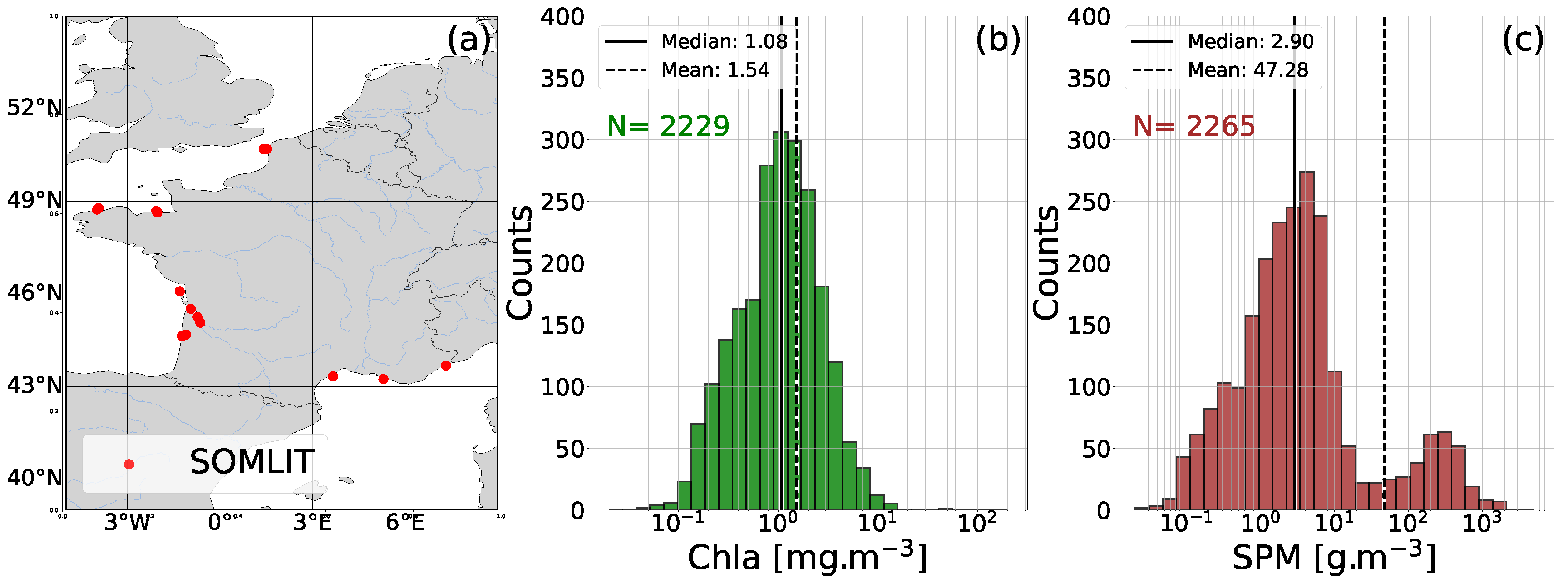
2.1. In Situ Data

Data from the French coastal monitoring network “Service d’Observation en Milieu Littoral” (SOMLIT) were used in the matchup analysis (https://www.somlit.fr/, accessed on 3 May 2024). This long-lasting in situ dataset, providing continuous bi-monthly data since 1997, is acquired using a standardized protocol. The dataset currently consists of twenty-two stations distributed along the French coastline, where sixteen parameters are measured or sampled [47]. The SPM concentration is determined by filtering a sufficient volume of water through pre-weighted GF/F filters (approximately 0.7 µm porosity) to deposit 0.5 to 1 mg of material on the filter, rinsing them with Milli-Q water to remove salts and drying the filters in a temperature-controlled oven at 50–70 °C for at least 6 h. Post-drying, filters are weighed again, and the SPM concentration is computed. The Chla concentration is measured by filtering from 0.1 to 1 L of seawater with GF/F filters (approximately 0.7 µm porosity), extracting pigments with 90% acetone, and measuring fluorescence before and after acidification. In this study, only surface measurements were selected, and the SPM data were quality controlled (retaining only data with quality flags 2, 6, and 7, corresponding to unique measurements, duplicate samples, and reliable measurements from an alternative protocol). After applying these criteria, 2265 and 2229 potential SPM and Chla matchups remained, respectively, with measurements being collected between September 2018 and July 2023. Figure 1 shows as red dots the locations of those in situ measurements in the French coastal waters. The Chla values vary from 0.04 mg·m⁻³ to 50.8 mg·m⁻³, with a mean value of 1.54 mg·m⁻³ (Figure 1b), while SPM values range from 0.01 g·m⁻³ to 1970.14 g·m⁻³, with a mean value of 47.28 g·m⁻³ (Figure 1c).

2.2. Satellite Data

2.2.1. COCTS

The Chinese Ocean Color and Temperature Scanner (COCTS) sensor has been in orbit aboard the HY-1C/D satellites since September 2018 for HY-1C and June 2020 for HY-1D, respectively. COCTS was firstly onboard the experimental ocean color satellite Haiyang-1A, launched in 2002, and has achieved significant improvements in its number of bands, swath width, and radiometric performance on the succeeding Haiyang-1B/C/D satellites. The sensor observes the Earth with a swath width of 3000 km and a spatial resolution of 1.1 km. COCTS comprises six visible bands and two near-infrared bands, i.e., 412 nm, 443 nm, 490 nm, 520 nm, 565 nm, 670 nm, 750 nm, and 865 nm [23]. The remote sensing data of COCTS on HY-1C/1D are available for registered users from the National Satellite Ocean Application Service (NSOAS) website (https://osdds.nsoas.org.cn/ (accessed on 10 May 2024)). Each file contains a five-minute granule of satellite data. L2A files contain $R_{rs}$ data and L2B files the derived biogeochemical products. A total of 1799 L2B files were downloaded for HY-1C, and 762 were downloaded for HY-1D. Notably, some L2A files required to derive the L2B files were missing on the NSOAS servers, reducing the potential number of matchups. Regarding the COCTS standard algorithms, Chla concentration is estimated with an OC4-like model [29], and SPM is derived using a proxy, deduced from four indices defined by combinations of reflectances at different bands [41]. However, the exact model formulations and their calibration coefficients are not publicly available. Several quality flags are included in the L2A and L2B files, such as atmospheric correction failure, sun glint, radiance saturation, high sensor view zenith angle, shallow water, or turbid water.

2.2.2. MODIS

The Moderate Resolution Imaging Spectroradiometer (MODIS) AQUA level 2 image used in this study, for a comparison with a COCTS image, was obtained from the NASA Ocean Color Archive (https://oceancolor.gsfc.nasa.gov, accessed on 7 February 2025). The MODIS AQUA sensor has been operational aboard NASA’s Earth Observing System (EOS/PM1) satellite since May 2002. The available spectral bands for this product are 412, 443, 469, 488, 531, 547, 555, 645, 667, and 678 nm.

2.3. Matchup Methodology

The matchup extraction was performed following the method of previously published works [45,48,49,50]. We considered 3 × 3 pixel windows, centered on the in situ sampling point, and matchups were selected according to the following criteria: (1) at least 6 valid pixels among the 9 pixels; (2) to ensure spatial homogeneity, the coefficient of variation (i.e., the ratio of the standard deviation over the mean value) of $R_{rs}$(565) within the window must be less than 20%; (3) the time difference between in situ and satellite measurements has to be lower than 3 h; and (4) the sun zenith angle has to be lower than 70°. Although this time window may be relatively large for SOMLIT stations located in dynamic coastal waters, we chose it to maximize the number of matchups [45,50]. Finally, for the matchups, SPM and Chla were extracted for the valid pixels in the 3 × 3 window, and the median value was calculated for comparison. A second stricter protocol was also applied by excluding matchups with negative $R_{rs}$ spectra in the visible spectrum.

2.4. Statistical Metrics

The performance of the SPM and Chla products was assessed using metrics calculated in the log-space, as this approach offers a more accurate evaluation due to the log-normal distribution of these parameters in natural environments [51]. Metrics based on the median were prioritized, as it is less affected by outliers [52,53]. The following metrics were analyzed, where $X^{est}$ represents the estimated value and $X^{obs}$ the in situ value of either SPM or Chla:

• Symmetric signed percentage bias (SSPB), representing a zero-centered percent bias that maintains symmetry between over- and under-estimation [53,54,55]. Negative values indicate under-estimation and positive over-estimation

$$SSPB=100\times sign\left(MdLQ\right)\times ({10}^{\left|MdLQ\right|}-1)$$

(1)

$$\mathrm{where}MdLQ=median\left(lo{g}_{10}(X^{est}/X^{obs})\right)$$

(2)

• Mean symmetric accuracy (MSA), representing a symmetric percentage error and penalizing over- and under-estimation in the same way [53,54,55]. This metric was designed to address the drawbacks of MAPE (mean absolute percentage error). Values closer to zero indicate better performance

$$MSA=100\times ({10}^{median\left(\right|lo{g}_{10}(X^{est}/X^{obs})\left|\right)}-1)$$

(3)

• Root mean square logarithmic error (“RMSLE”), quantifying the deviation of estimated values from the measured ones, incorporating a quadratic penalty for larger errors. Values closer to zero indicate better performance

$$RMSLE=\sqrt{{\displaystyle \frac{{\sum }_{i=1}^n{(lo{g}_{10}\left(X_i^{\mathrm{est}}\right)-lo{g}_{10}\left(X_i^{\mathrm{obs}}\right))}^2}{n}}}$$

(4)

• The Slope from a type II linear regression on the log-transformed data accounts for errors in both observed and estimated variables.

$$lo{g}_{10}\left(X^{est}\right)=slope\times lo{g}_{10}\left(X^{obs}\right)+intercept$$

(5)

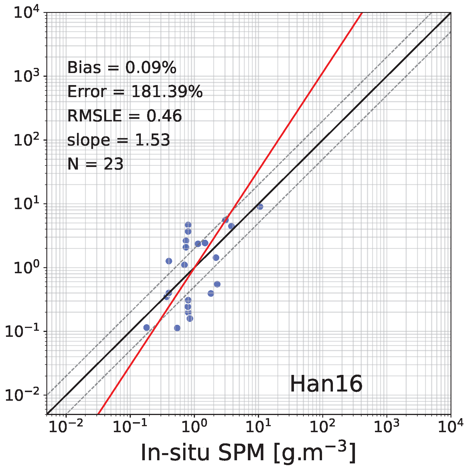
2.5. SPM Model Tested

In this study, the standard COCTS SPM product was compared with the semi-analytical approach proposed by Han et al. [39] (hereafter referred to as Han16). This model was chosen because it performs well over a wide range of SPM concentrations [45] and was also tuned for the band 670, making it applicable to COCTS. It combines two equations through weights, one tuned for low concentrations of SPM and one tuned for high concentrations. The development dataset spans 4 orders of magnitude, ranging from 0.15 to 2626 g·m⁻³. Both equations are combined when 0.03 < $R_{rs}\left(670\right)$ < 0.04 sr⁻¹:

$$SP{M}_{low}={\displaystyle \frac{391.161\times \pi \times R_{rs}\left(670\right)}{1-\frac{\pi \times R_{rs}\left(670\right)}{0.5}}}\mathrm{if}{R}_{rs}\left(670\right)<0.03s{r}^{-1}$$

(6)

$$SP{M}_{high}={\displaystyle \frac{1336.584\times \pi \times R_{rs}\left(670\right)}{1-\frac{\pi \times R_{rs}\left(670\right)}{0.3864}}}\mathrm{if}{R}_{rs}\left(670\right)>0.04s{r}^{-1}$$

(7)

$$SPM={\displaystyle \frac{W_{low}\times SP{M}_{low}+W_{high}\times SP{M}_{high}}{W_{low}+W_{high}}}$$

(8)

$$\begin{array}{cc}\hfill \mathrm{where}{W}_{\mathrm{low}}& ={log}_{10}\left(0.04\right)-{log}_{10}\left(R_{\mathrm{rs}}\left(670\right)\right),\hfill \\ \hfill W_{\mathrm{high}}& ={log}_{10}\left(R_{\mathrm{rs}}\left(670\right)\right)-{log}_{10}\left(0.03\right)\hfill \end{array}$$

(9)

3. Results

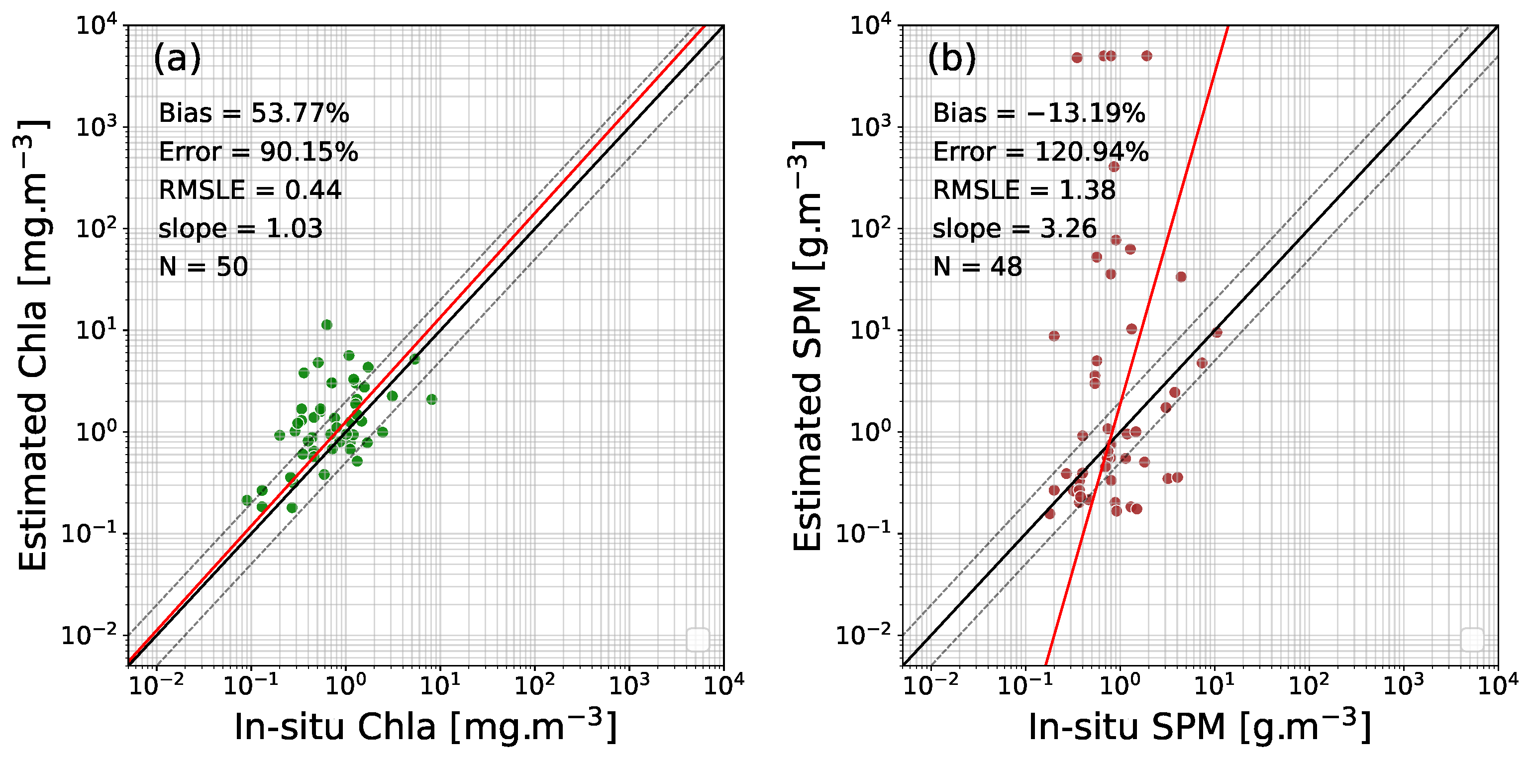
3.1. Matchup Exercise

The scatterplots in Figure 2 show the performance of COCTS standard algorithms in estimating Chla and SPM concentrations from $R_{rs}$ radiometric data. Out of the 90 potential matchups between L2B COCTS images and SOMLIT data, only 75 of the corresponding L2A files ($R_{rs}$ data) were available on the NSOAS server, reducing the number of matchups. We found 50 matchups for Chla, corresponding to in situ concentrations varying between 0.09 and 8.12 mg·m⁻³ (Figure 2a). The scatterplot shows several outliers, mostly located above the unity line, leading to a Bias (SSPB) of 53.77%, an Error (MSA) of 90.15%, and an RMSLE of 0.44. Remotely estimated and in situ values are overall well aligned, with a Slope of 1.03. On the other hand, Figure 2b shows a more dispersed distribution of 48 matchup points for SPM, with in situ concentrations varying between 0.18 g·m⁻³ and 10.52 g·m⁻³. The standard algorithm significantly overestimated SPM, leading to an Error of 120.94%, an RMSLE of 1.38, and a Slope of 3.26. The model showed a saturation value of 5011.87 g·m⁻³, which was reached in three matchups without raising any of the existing flags in the L2 product. While we observe clear differences between the performances of Chla and SPM standard models in this figure, the matchups with those variables correspond to measurements conducted at the same time and location. Thus, both models used the same radiometric data as input, and it suggests that the issues related with the SPM product might not be due to the $R_{rs}$ data. The other overestimated SPM values also presented no flags.

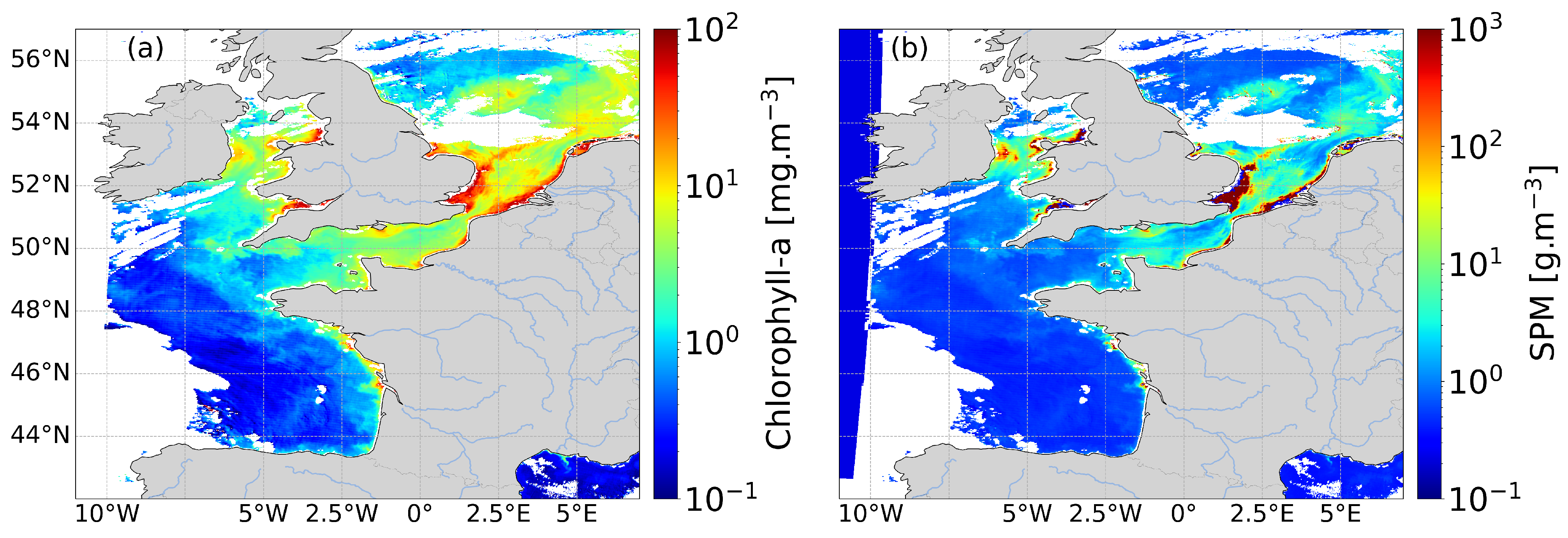
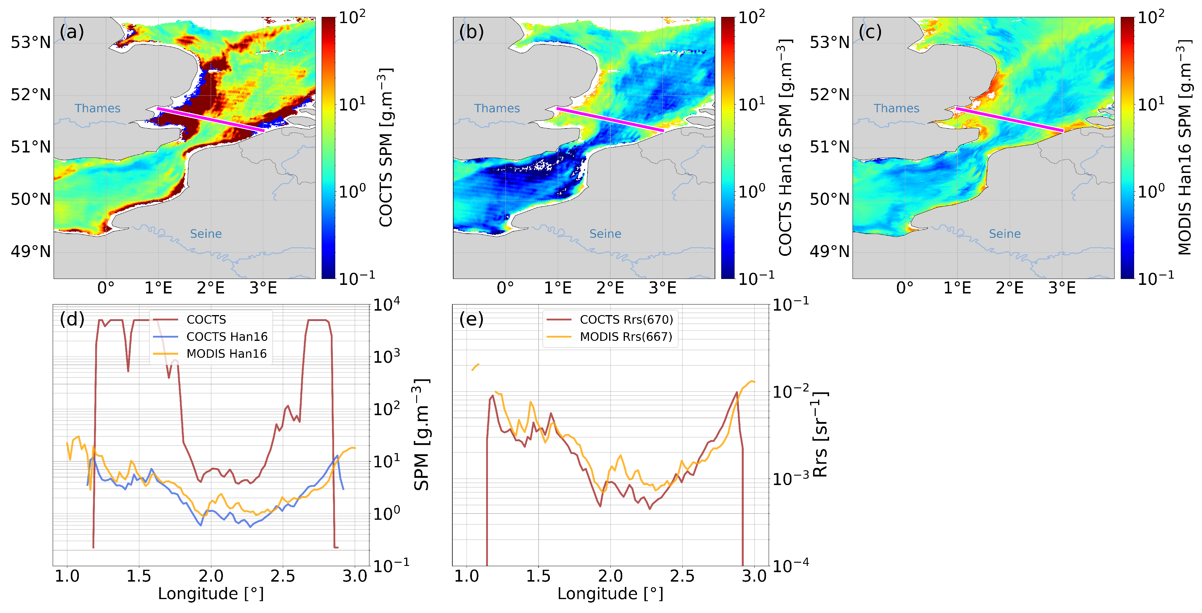
3.2. Chla and SPM Maps Assessment

Figure 3 shows an example of a HY-1C/COCTS image on 27 September 2018, taken above Northwestern Europe. We selected this image as it featured small cloud cover and a great diversity of SPM concentrations and gradients. Both Chla and SPM fields exhibited low concentrations offshore in the Bay of Biscay and the Atlantic Ocean and higher values in the English Channel, the North Sea, and river estuaries. Chla values were reasonable across the image, with concentrations of about 0.3 mg·m⁻³ in the Atlantic Ocean and 2.5 mg·m⁻³ in the English Channel. Chla reached about 30 mg·m⁻³ in the Thames River plume, where such concentrations are expected [56]. On the other hand, the SPM product exhibited extreme values in coastal and estuarine waters. As an example, concentrations of 5011.87 g·m⁻³ were found in the plumes of rivers like Seine or Thames, as well as along the coasts of Belgium and the Netherlands. However, SPM can only reach about 500 g·m⁻³ in the Thames estuary [57] and 200 g·m⁻³ for the Seine River [58]. Although some of these pixels were flagged as “turbid waters”, not all were. The same pixels showed realistic Chla values, suggesting that the issue likely originates from the SPM model. The SPM gradients near those pixels were very strong, increasing from values of 3 g·m⁻³ to 5011.87 g·m⁻³ within less than 6 km. Moreover, pixels with SPM values of 0.22 g·m⁻³ were found between land and saturated pixels, as shown in Figure 3b in the Thames estuary, and also flagged as “turbid waters” and “spare”. They corresponded to saturated Chla values at 64.0 mg·m⁻³. Finally, we also observed a blue band on the left of the SPM image (Figure 3b), along the 10°W meridian, corresponding to a constant SPM value of 0.22 g·m⁻³, which was not visible in the Chla image. However, they were flagged as pixels with a satellite viewing angle greater than 60°, and matchups with those pixels should not be considered. The above-mentioned issues were observed in many other COCTS images.

4. Discussion

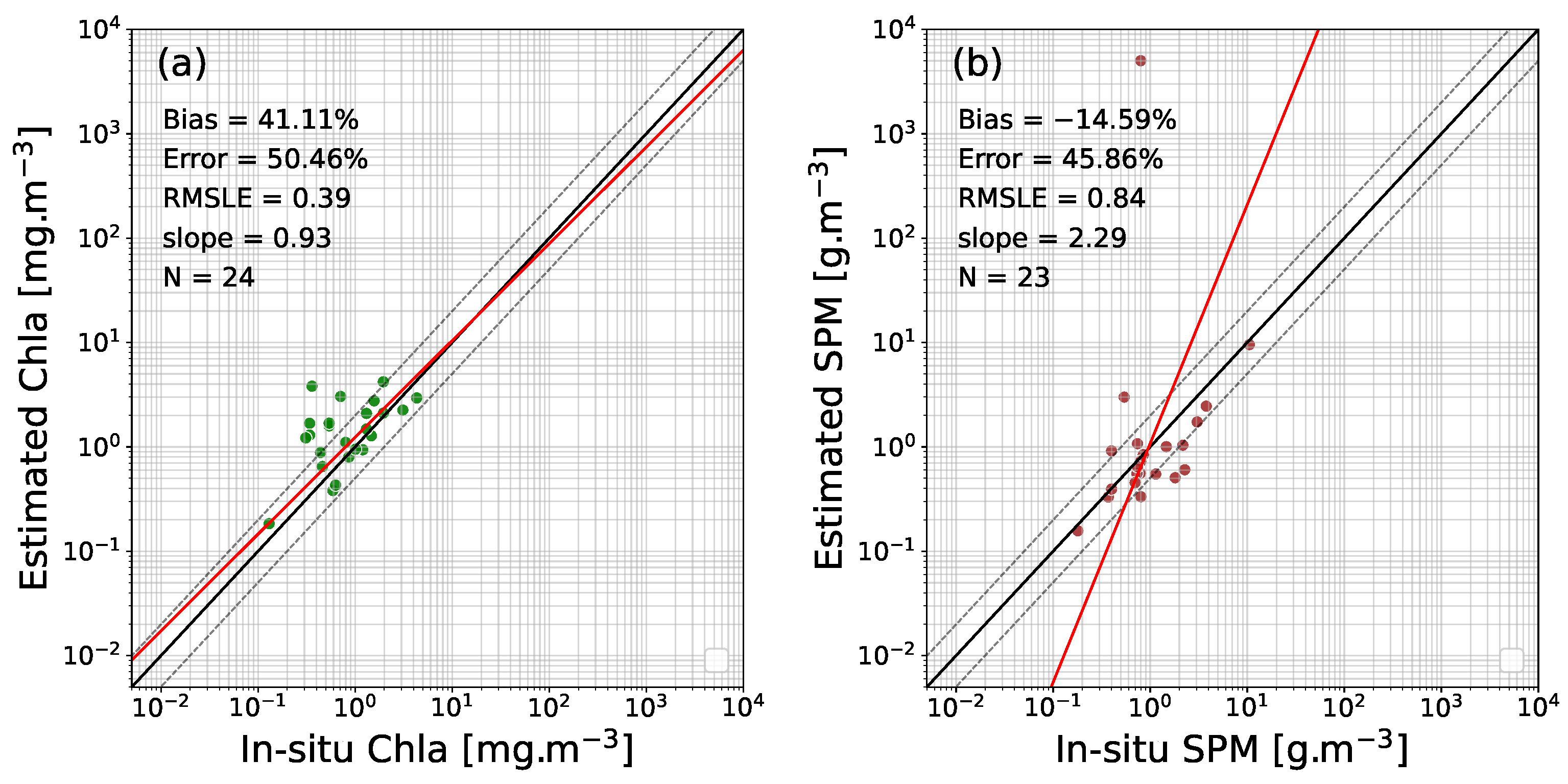
4.1. A Stricter Matchup Exercise

To investigate the causes of SPM overestimation, we removed the matchups presenting negative $R_{rs}$ values in the visible part of the COCTS spectra (Figure 4). The number of matchups decreased to 24 for Chla and 23 for SPM, but the overall quality improved. They cover relatively clear waters: Chla varied from 0.13 to 4.31 mg·m⁻³ and SPM from 0.18 to 10.52 g·m⁻³, with respective median values of 0.75 mg·m⁻³ and 0.8 g·m⁻³. This filtering step eliminated strong outliers for Chla, now retrieved with a Bias of 41.11%, an Error of 50.46%, an RMSLE of 0.39, and a Slope of 0.93 (Figure 4a). Concerning SPM, this filtering significantly altered the matchup results, removing most of the outliers. The retrieval accuracy increased, with a new Bias value of −14% and an Error of 45.86%. However, one outlier with a value of 5011.87 g·m⁻³ was retained, inducing a high Slope value of 2.29 and an RMSLE of 0.84. Even though the associated $R_{rs}$ data did not present negative values in this case, the matchup is located in a part of the image where $R_{rs}$ values suddenly decrease from one or two orders of magnitude for all bands, compared with surrounding pixels. Excluding this outlier yielded improved statistics; the statistical metrics changed to −22.7% for the Bias, 45.5% for the Error, 0.29 for the RMSLE, and 0.96 for the Slope. One of the limitations of this study lies in the relatively small number of matchups, which may limit the representativeness of our matchup dataset. However, they provide valuable regional information on the accuracy of SPM and Chla COCTS products over specific ranges of concentrations. Moreover, the accuracy and Bias metrics used here are based on the median, which mitigates the impacts of potential outliers within the matchups [51,53].

4.2. Inter-Comparison with Another SPM Model

We applied the Han16 model to estimate SPM from the $R_{rs}$ corresponding to the 23 matchups with SOMLIT to compare with the standard COCTS product. Figure 5 shows that the outlier present for the COCTS product is not present in the scatterplot for Han16, further suggesting that the issue originates from the COCTS SPM model for this outlier and not the $R_{rs}$ product. For those matchups, Han16 retrieved SPM with a negligible Bias, an Error of 181.39%, an RMSLE of 0.46, and a Slope of 1.53. Its contrasted performance might result from the fact that the model is based on $R_{rs}$(670), whose signal is weak in relatively clear waters. Ref. [45] showed that Han16 tends to output high estimation errors when the SPM concentrations are about 1 g·m⁻³ or lower. When considering only the matchups with in situ SPM values below 1 g·m⁻³, the Bias and Error for the COCTS product were −9.79% and 31.39%, and the ones for Han16 are 0.09% and 215.96%. However, when considering matchups with SPM values greater than 1 g·m⁻³, the Bias and Error of the COCTS product are −91.1% and 91.1%, and the ones for Han16 are 0.54% and 73.82%.

To extend the comparison, we applied Han16 to estimate the SPM for the COCTS scene shown in Figure 3. Figure 6 presents a subset centered on the Thames estuary, showing the COCTS SPM (Figure 6a), Han16-derived SPM from COCTS (Figure 6b), and a concentration profile along a transect from the Thames estuary to the Belgian coast. A MODIS/AQUA image of the same day was selected as a comparison, as it is a widely used and well-validated sensor [17,49,59]. SPM derived from MODIS (Figure 6c) was also estimated with Han16, with coefficients computed for this sensor [39]. A comparison of the three maps and transect data revealed that the COCTS product systematically presented higher values than the SPM estimated with Han16 from COCTS or MODIS. As described previously, COCTS SPM values exceeded 1000 g·m⁻³ in most of the Thames plume waters and along the Belgium coastline, reaching up to 5011.87 g·m⁻³. In the same part of the section, Han16-derived SPM from both COCTS and MODIS varied between 3 and 20 g·m⁻³, showing great differences between the three products. The COCTS Han16 and MODIS Han16 transects also align well (Figure 6e), with minor differences likely attributable to the fact that the COCTS image was taken at 10h30 and the MODIS one at 12h40. This is consistent with the highly dynamic nature of coastal waters, where strong currents, tides, and fronts can be observed, and where SPM can thus present a high temporal variability [60]. Finally, the values of $R_{rs}\left(670\right)$ for COCTS and $R_{rs}\left(667\right)$ for MODIS along this same transect were in good agreement, suggesting that the COCTS SPM overestimation originates from the SPM algorithm used and not from errors in the atmospheric correction procedure.

5. Conclusions

In this study, we evaluated the quality of the standard COCTS Chla and SPM products over French coastal waters for the first time. While the Chla product showed robustness, the SPM product must be interpreted with caution. The 23 and 24 high-confidence matchups for SPM and Chla, respectively, only covered moderately turbid waters, with concentrations varying from 0.13 to 4.31 mg·m⁻³ for Chla and from 0.18 to 10.52 g·m⁻³ for SPM and respective median values of 0.75 mg·m⁻³ and 0.80 g·m⁻³. Over this dynamic range, the errors associated with Chla and SPM retrievals reached 50.46% and 45.86%, respectively. However, several issues related to the COCTS SPM product were pointed out: the matchup exercise and a comparison with the SPM model from Han et al. [39] showed that the COCTS SPM model seems to have difficulties over a wide range of concentrations and tends to saturate. This saturation leads to unrealistically strong SPM gradients in the images and limits the potential use of this product in river estuaries or turbid areas. This study represents an initial regional assessment of COCTS-derived standard products. One limitation of this study is the relatively small number of matchups, all confined to a single coastal region, which may constrain the overall representativeness of the dataset. Nevertheless, these matchups offer valuable regional insights into the accuracy of the COCTS-derived SPM and Chla products, particularly within those specific concentration ranges. These findings have important ecological implications. The evaluation results of the COCTS Chla product suggest it can serve as a useful tool for monitoring phytoplankton dynamics in oligotrophic to mesotrophic coastal waters. Such environments are particularly sensitive to nutrient loading and climatic variability, making robust spaceborne Chla estimations valuable for monitoring ecological status and for the detection of algal blooms and water quality changes [61]. On the other hand, the poor performance of the COCTS SPM product in similar conditions limits its ecological utility, particularly for applications involving turbidity monitoring, sediment transport, light availability assessments, and implications for aquaculture [11,62]. SPM plays a critical role in modulating light penetration, influencing benthic habitat suitability, and transporting nutrients and contaminants [9,63]. While the COCTS Chla standard product shows promise for estimating biological productivity, additional algorithm improvements are needed to fully support an integrated ecological monitoring in optically complex coastal waters. Finally, more evaluation exercises are necessary to validate both COCTS biogeochemical and $R_{rs}$ products over a greater diversity of optical water types. Future work should focus on expanding the number of matchups in different regions of the world, but also in different concentration ranges, to validate these products under specific conditions, such as in turbid or eutrophic waters.

References

1. Tavora, J.; Boss, E.; Doxaran, D.; Hill, P. An Algorithm to Estimate Suspended Particulate Matter Concentrations and Associated Uncertainties from Remote Sensing Reflectance in Coastal Environments. Remote Sens. 2020, 12, 2172. [Google Scholar] [CrossRef]
2. Hourany, R.E.; Mejia, C.; Faour, G.; Crépon, M.; Thiria, S. Evidencing the Impact of Climate Change on the Phytoplankton Community of the Mediterranean Sea Through a Bioregionalization Approach. J. Geophys. Res. Ocean. 2021, 126, e2020JC016808. [Google Scholar] [CrossRef]
3. Loisel, H.; Duforêt-Gaurier, L.; Tran, T.K.; Jorge, D.S.F.; Steinmetz, F.; Mangin, A.; Bretagnon, M.; Fanton, O.H. Characterization of the Organic vs. Inorganic Fraction of Suspended Particulate Matter in Coastal Waters Based on Ocean Color Radiometry Remote Sensing; Copernicus Publications: Göttingen, Germany, 2023; Volume 1-osr7, pp. 1–12. [Google Scholar] [CrossRef]
4. Cael, B.B.; Bisson, K.; Boss, E.; Dutkiewicz, S.; Henson, S. Global climate-change trends detected in indicators of ocean ecology. Nature 2023, 619, 551–554. [Google Scholar] [CrossRef] [PubMed]
5. Antoine, D.; André, J.; Morel, A. Oceanic primary production: 2. Estimation at global scale from satellite (Coastal Zone Color Scanner) chlorophyll. Glob. Biogeochem. Cycles 1996, 10, 57–69. [Google Scholar] [CrossRef]
6. Loisel, H.; Vantrepotte, V.; Ouillon, S.; Ngoc, D.D.; Herrmann, M.; Tran, V.; Mériaux, X.; Dessailly, D.; Jamet, C.; Duhaut, T.; et al. Assessment and analysis of the chlorophyll-a concentration variability over the Vietnamese coastal waters from the MERIS ocean color sensor (2002–2012). Remote Sens. Environ. 2017, 190, 217–232. [Google Scholar] [CrossRef]
7. Pahlevan, N.; Smith, B.; Schalles, J.; Binding, C.; Cao, Z.; Ma, R.; Alikas, K.; Kangro, K.; Gurlin, D.; Hà, N.; et al. Seamless retrievals of chlorophyll-a from Sentinel-2 (MSI) and Sentinel-3 (OLCI) in inland and coastal waters: A machine-learning approach. Remote Sens. Environ. 2020, 240, 111604. [Google Scholar] [CrossRef]
8. van Oostende, M.; Hieronymi, M.; Krasemann, H.; Baschek, B. Global ocean colour trends in biogeochemical provinces. Front. Mar. Sci. 2023, 10, 1052166. [Google Scholar] [CrossRef]
9. Miller, R.L.; Cruise, J.F. Effects of suspended sediments on coral growth: Evidence from remote sensing and hydrologic modeling. Remote Sens. Environ. 1995, 53, 177–187. [Google Scholar] [CrossRef]
10. Turner, A.; Millward, G.E. Suspended Particles: Their Role in Estuarine Biogeochemical Cycles. Estuarine Coast Shelf Sci. 2002, 55, 857–883. [Google Scholar] [CrossRef]
11. Gernez, P.; Barillé, L.; Lerouxel, A.; Mazeran, C.; Lucas, A.; Doxaran, D. Remote sensing of suspended particulate matter in turbid oyster-farming ecosystems. J. Geophys. Res. Ocean. 2014, 119, 7277–7294. [Google Scholar] [CrossRef]
12. Loisel, H.; Mangin, A.; Vantrepotte, V.; Dessailly, D.; Dinh, D.N.; Garnesson, P.; Ouillon, S.; Lefebvre, J.P.; Mériaux, X.; Phan, T.M. Variability of suspended particulate matter concentration in coastal waters under the Mekong’s influence from ocean color (MERIS) remote sensing over the last decade. Remote Sens. Environ. 2014, 150, 218–230. [Google Scholar] [CrossRef]
13. Crossland, C.J.; Baird, D.; Ducrotoy, J.P.; Lindeboom, H.; Buddemeier, R.W.; Dennison, W.C.; Maxwell, B.A.; Smith, S.V.; Swaney, D.P. The Coastal Zone—A Domain of Global Interactions; Springer: Berlin/Heidelberg, Germany, 2005; pp. 1–37. [Google Scholar] [CrossRef]
14. Gleason, M.G.; Reynolds, M.D.; Heady, W.N.; Easterday, K.; Morrison, S.A. The importance of identifying and protecting coastal wildness. Front. Conserv. Sci. 2023, 4, 1224618. [Google Scholar] [CrossRef]
15. Melet, A.; Teatini, P.; Cozannet, G.L.; Jamet, C.; Conversi, A.; Benveniste, J.; Almar, R. Earth Observations for Monitoring Marine Coastal Hazards and Their Drivers. Surv. Geophys. 2020, 41, 1489–1534. [Google Scholar] [CrossRef]
16. Serafy, G.Y.E.; Schaeffer, B.A.; Neely, M.B.; Spinosa, A.; Odermatt, D.; Weathers, K.C.; Baracchini, T.; Bouffard, D.; Carvalho, L.; Conmy, R.N.; et al. Integrating Inland and Coastal Water Quality Data for Actionable Knowledge. Remote Sens. 2021, 13, 2899. [Google Scholar] [CrossRef] [PubMed]
17. Doxaran, D.; Lamquin, N.; Park, Y.J.; Mazeran, C.; Ryu, J.H.; Wang, M.; Poteau, A. Retrieval of the seawater reflectance for suspended solids monitoring in the East China Sea using MODIS, MERIS and GOCI satellite data. Remote Sens. Environ. 2014, 146, 36–48. [Google Scholar] [CrossRef]
18. Loisel, H.; Vantrepotte, V.; Jamet, C.; Ngoc Dat, D. Challenges and New Advances in Ocean Color Remote Sensing of Coastal Waters. In Topics in Oceanography; InTech: Rijeka, Croatia, 2013. [Google Scholar] [CrossRef]
19. Jiang, X.; Yin, X.; Guan, L.; Wang, Z.; Lv, L.; Liu, M. Global ocean observations and applications by China’s ocean satellite constellation. Intell. Mar. Technol. Syst. 2023, 1, 6. [Google Scholar] [CrossRef]
20. Ye, X.; Liu, J.; Lin, M.; Ding, J.; Zou, B.; Song, Q. Global Ocean Chlorophyll-a Concentrations Derived from COCTS Onboard the HY-1C Satellite and Their Preliminary Evaluation. IEEE Trans. Geosci. Remote Sens. 2021, 59, 9914–9926. [Google Scholar] [CrossRef]
21. Li, H.; He, X.; Ding, J.; Bai, Y.; Wang, D.; Gong, F.; Li, T. The Inversion of HY-1C-COCTS Ocean Color Remote Sensing Products from High-Latitude Seas. Remote Sens. 2022, 14, 5722. [Google Scholar] [CrossRef]
22. Mao, Z.; Tao, B.; Chen, J.; Chen, P.; Hao, Z.; Zhu, Q.; Huang, H. A Layer Removal Scheme for Atmospheric Correction of Satellite Ocean Color Data in Coastal Regions. IEEE Trans. Geosci. Remote Sens. 2021, 59, 1382–1391. [Google Scholar] [CrossRef]
23. Mao, Z.; Zhang, Y.; Tao, B.; Chen, J.; Hao, Z.; Zhu, Q.; Huang, H. The Atmospheric Correction of COCTS on the HY-1C and HY-1D Satellites. Remote Sens. 2022, 14, 6372. [Google Scholar] [CrossRef]
24. Xu, Y.; He, X.; Bai, Y.; Wang, D.; Zhu, Q.; Ding, X. Evaluation of Remote-Sensing Reflectance Products from Multiple Ocean Color Missions in Highly Turbid Water (Hangzhou Bay). Remote Sens. 2021, 13, 4267. [Google Scholar] [CrossRef]
25. Chen, S.; Du, K.; Lee, Z.; Liu, J.; Song, Q.; Xue, C.; Wang, D.; Lin, M.; Tang, J.; Ma, C. Performance of COCTS in Global Ocean Color Remote Sensing. IEEE Trans. Geosci. Remote Sens. 2021, 59, 1634–1644. [Google Scholar] [CrossRef]
26. Gordon, H.R.; Wang, M. Retrieval of water-leaving radiance and aerosol optical thickness over the oceans with SeaWiFS: A preliminary algorithm. Appl. Opt. 1994, 33, 443–452. [Google Scholar] [CrossRef] [PubMed]
27. Gordon, H.R.; Ahn, J.H. Evolution of Ocean Color Atmospheric Correction: 1970–2005. Remote Sens. 2021, 13, 5051. [Google Scholar] [CrossRef]
28. O’Reilly, J.E.; Maritorena, S.; Mitchell, B.G.; Siegel, D.A.; Carder, K.L.; Garver, S.A.; Kahru, M.; McClain, C. Ocean color chlorophyll algorithms for SeaWiFS. J. Geophys. Res. Ocean. 1998, 103, 24937–24953. [Google Scholar] [CrossRef]
29. O’Reilly, J.E.; Werdell, P.J. Chlorophyll algorithms for ocean color sensors—OC4, OC5 and OC6. Remote Sens. Environ. 2019, 229, 32–47. [Google Scholar] [CrossRef] [PubMed]
30. Mélin, F.; Vantrepotte, V. How optically diverse is the coastal ocean? Remote Sens. Environ. 2015, 160, 235–251. [Google Scholar] [CrossRef]
31. Gitelson, A.A.; Schalles, J.F.; Hladik, C.M. Remote chlorophyll-a retrieval in turbid, productive estuaries: Chesapeake Bay case study. Remote Sens. Environ. 2007, 109, 464–472. [Google Scholar] [CrossRef]
32. Gurlin, D.; Gitelson, A.A.; Moses, W.J. Remote estimation of chl-a concentration in turbid productive waters—Return to a simple two-band NIR-red model? Remote Sens. Environ. 2011, 115, 3479–3490. [Google Scholar] [CrossRef]
33. Tran, M.D.; Vantrepotte, V.; Loisel, H.; Oliveira, E.N.; Tran, K.T.; Jorge, D.; Mériaux, X.; Paranhos, R. Band Ratios Combination for Estimating Chlorophyll-a from Sentinel-2 and Sentinel-3 in Coastal Waters. Remote Sens. 2023, 15, 1653. [Google Scholar] [CrossRef]
34. Gross, L.; Thiria, S.; Frouin, R.; Mitchell, B.G. Artificial neural networks for modeling the transfer function between marine reflectance and phytoplankton pigment concentration. J. Geophys. Res. Ocean. 2000, 105, 3483–3495. [Google Scholar] [CrossRef]
35. D’Alimonte, D.; Zibordi, G. Phytoplankton determination in an optically complex coastal region using a multilayer perceptron neural network. IEEE Trans. Geosci. Remote Sens. 2003, 41, 2861–2868. [Google Scholar] [CrossRef]
36. Nechad, B.; Ruddick, K.G.; Park, Y. Calibration and validation of a generic multisensor algorithm for mapping of total suspended matter in turbid waters. Remote Sens. Environ. 2010, 114, 854–866. [Google Scholar] [CrossRef]
37. Jiang, D.; Matsushita, B.; Pahlevan, N.; Gurlin, D.; Lehmann, M.K.; Fichot, C.G.; Schalles, J.; Loisel, H.; Binding, C.; Zhang, Y.; et al. Remotely estimating total suspended solids concentration in clear to extremely turbid waters using a novel semi-analytical method. Remote Sens. Environ. 2021, 258, 112386. [Google Scholar] [CrossRef]
38. Jiang, D.; Matsushita, B.; Pahlevan, N.; Gurlin, D.; Fichot, C.G.; Harringmeyer, J.; Sent, G.; Brito, A.C.; Brotas, V.; Werther, M.; et al. Estimating the concentration of total suspended solids in inland and coastal waters from Sentinel-2 MSI: A semi-analytical approach. ISPRS J. Photogramm. Remote Sens. 2023, 204, 362–377. [Google Scholar] [CrossRef]
39. Han, B.; Loisel, H.; Vantrepotte, V.; Mériaux, X.; Bryère, P.; Ouillon, S.; Dessailly, D.; Xing, Q.; Zhu, J. Development of a Semi-Analytical Algorithm for the Retrieval of Suspended Particulate Matter from Remote Sensing over Clear to Very Turbid Waters. Remote Sens. 2016, 8, 211. [Google Scholar] [CrossRef]
40. Balasubramanian, S.V.; Pahlevan, N.; Smith, B.; Binding, C.; Schalles, J.; Loisel, H.; Gurlin, D.; Greb, S.; Alikas, K.; Randla, M.; et al. Robust algorithm for estimating total suspended solids (TSS) in inland and nearshore coastal waters. Remote Sens. Environ. 2020, 246, 111768. [Google Scholar] [CrossRef]
41. Mao, Z.; Chen, J.; Pan, D.; Tao, B.; Zhu, Q. A regional remote sensing algorithm for total suspended matter in the East China Sea. Remote Sens. Environ. 2012, 124, 819–831. [Google Scholar] [CrossRef]
42. Moutier, W.; Thomalla, S.J.; Bernard, S.; Wind, G.; Ryan-Keogh, T.J.; Smith, M.E. Evaluation of Chlorophyll-a and POC MODIS Aqua Products in the Southern Ocean. Remote Sens. 2019, 11, 1793. [Google Scholar] [CrossRef]
43. Delgado, A.L.; Pratolongo, P.D.; Dogliotti, A.I.; Arena, M.; Celleri, C.; Cardona, J.E.G.; Martinez, A. Evaluation of MODIS-Aqua and OLCI Chlorophyll-a products in contrasting waters of the Southwestern Atlantic Ocean. Ocean Coast. Res. 2021, 69, e21007. [Google Scholar] [CrossRef]
44. Cao, Z.; Ma, R.; Pahlevan, N.; Liu, M.; Melack, J.M.; Duan, H.; Xue, K.; Shen, M. Evaluating and Optimizing VIIRS Retrievals of Chlorophyll-a and Suspended Particulate Matter in Turbid Lakes Using a Machine Learning Approach. IEEE Trans. Geosci. Remote Sens. 2022, 60, 4211417. [Google Scholar] [CrossRef]
45. Subirade, C.; Jamet, C.; Duy Tran, M.; Vantrepotte, V.; Han, B. Evaluation of twelve algorithms to estimate suspended particulate matter from OLCI over contrasted coastal waters. Opt. Express 2024, 32, 45719–45744. [Google Scholar] [CrossRef]
46. Yang, G.; Ye, X.; Xu, Q.; Yin, X.; Xu, S. Sea Surface Chlorophyll-a Concentration Retrieval from HY-1C Satellite Data Based on Residual Network. Remote Sens. 2023, 15, 3696. [Google Scholar] [CrossRef]
47. Breton, E.; Savoye, N.; Rimmelin-Maury, P.; Sautour, B.; Goberville, E.; Lheureux, A.; Cariou, T.; Ferreira, S.; Agogué, H.; Alliouane, S.; et al. Data quality control considerations in multivariate environmental monitoring: Experience of the French coastal network SOMLIT. Front. Mar. Sci. 2023, 10, 1135446. [Google Scholar] [CrossRef]
48. Bailey, S.W.; Werdell, P.J. A multi-sensor approach for the on-orbit validation of ocean color satellite data products. Remote Sens. Environ. 2006, 102, 12–23. [Google Scholar] [CrossRef]
49. Goyens, C.; Jamet, C.; Schroeder, T. Evaluation of four atmospheric correction algorithms for MODIS-Aqua images over contrasted coastal waters. Remote Sens. Environ. 2013, 131, 63–75. [Google Scholar] [CrossRef]
50. EUMETSAT. Recommendations for Sentinel-3 OLCI Ocean Colour Product Validations in Comparison with in situ Measurements–Matchup Protocols. EUM/SEN3/D. Technical Report v7, EUMETSAT, 2021. Available online: https://user.eumetsat.int/s3/eup-strapi-media/Recommendations_for_Sentinel_3_OLCI_Ocean_Colour_product_validations_in_comparison_with_in_situ_measurements_Matchup_Protocols_V8_B_e6c62ce677.pdf (accessed on 12 January 2025).
51. Stumpf, R.P.; Loftin, K.A.; Werdell, P.J.; Seegers, B.N.; Schaeffer, B.A. Performance metrics for the assessment of satellite data products: An ocean color case study. Opt. Express 2018, 26, 7404–7422. [Google Scholar] [CrossRef] [PubMed]
52. Leys, C.; Ley, C.; Klein, O.; Bernard, P.; Licata, L. Detecting outliers: Do not use standard deviation around the mean, use absolute deviation around the median. J. Exp. Soc. Psychol. 2013, 49, 764–766. [Google Scholar] [CrossRef]
53. Morley, S.K.; Brito, T.V.; Welling, D.T. Measures of Model Performance Based On the Log Accuracy Ratio. Space Weather 2018, 16, 69–88. [Google Scholar] [CrossRef]
54. Smith, B.; Pahlevan, N.; Schalles, J.; Ruberg, S.; Errera, R.; Ma, R.; Giardino, C.; Bresciani, M.; Barbosa, C.; Moore, T.; et al. A Chlorophyll-a Algorithm for Landsat-8 Based on Mixture Density Networks. Front. Remote Sens. 2021, 1, 623678. [Google Scholar] [CrossRef]
55. Pahlevan, N.; Smith, B.; Alikas, K.; Anstee, J.; Barbosa, C.; Binding, C.; Bresciani, M.; Cremella, B.; Giardino, C.; Gurlin, D.; et al. Simultaneous retrieval of selected optical water quality indicators from Landsat-8, Sentinel-2, and Sentinel-3. Remote Sens. Environ. 2022, 270, 112860. [Google Scholar] [CrossRef]
56. Weston, K.; Greenwood, N.; Fernand, L.; Pearce, D.J.; Sivyer, D.B. Environmental controls on phytoplankton community composition in the Thames plume, U.K. J. Sea Res. 2008, 60, 262–270. [Google Scholar] [CrossRef]
57. Uncles, R.J.; Mitchell, S.B. Turbidity in the Thames Estuary: How turbid do we expect it to be? Hydrobiologia 2011, 672, 91–103. [Google Scholar] [CrossRef]
58. Guézennec, L.; Lafite, R.; Dupont, J.P.; Meyer, R.; Boust, D. Hydrodynamics of suspended particulate matter in the tidal freshwater zone of a macrotidal estuary (the Seine Estuary, France). Estuaries 1999, 22, 717–727. [Google Scholar] [CrossRef]
59. Cao, Z.; Hu, C.; Ma, R.; Duan, H.; Liu, M.; Loiselle, S.; Song, K.; Shen, M.; Liu, D.; Xue, K. MODIS observations reveal decrease in lake suspended particulate matter across China over the past two decades. Remote Sens. Environ. 2023, 295. [Google Scholar] [CrossRef]
60. Vantrepotte, V.; Loisel, H.; Dessailly, D.; Mériaux, X. Optical classification of contrasted coastal waters. Remote Sens. Environ. 2012, 123, 306–323. [Google Scholar] [CrossRef]
61. Bricker, S.; Longstaff, B.; Dennison, W.; Jones, A.; Boicourt, K.; Wicks, C.; Woerner, J. Effects of nutrient enrichment in the nation’s estuaries: A decade of change. Harmful Algae 2008, 8, 21–32. [Google Scholar] [CrossRef]
62. Bilotta, G.S.; Brazier, R.E. Understanding the influence of suspended solids on water quality and aquatic biota. Water Res. 2008, 42, 2849–2861. [Google Scholar] [CrossRef] [PubMed]
63. Kroon, F.J.; Kuhnert, P.M.; Henderson, B.L.; Wilkinson, S.N.; Kinsey-Henderson, A.; Abbott, B.; Brodie, J.E.; Turner, R.D. River loads of suspended solids, nitrogen, phosphorus and herbicides delivered to the Great Barrier Reef lagoon. Mar. Pollut. Bull. 2012, 65, 167–181. [Google Scholar] [CrossRef] [PubMed]
Figure 1. (a) Spatial distribution of the SOMLIT network stations for which in situ Chla and SPM measurements were used in this study; (b) corresponding Chla frequency distribution; and (c) corresponding SPM frequency distribution.
Remotesensing 17 02516 g001
Figure 2. SOMLIT matchups with COCTS for (a) Chla and (b) SPM. Matchups with COCTS spectra presenting negative values in the visible spectrum were kept. The red lines correspond to a type II linear regression between in-situ and estimated concentrations.
Remotesensing 17 02516 g002
Figure 3. HY1C/COCTS L2 image of Northwest Europe, on 27 September 2018, of (a) Chla and (b) SPM.
Remotesensing 17 02516 g003
Figure 4. SOMLIT matchups with COCTS for (a) Chla and (b) SPM. Matchups with COCTS spectra presenting negative values in the visible were excluded. The red lines correspond to a type II linear regression between in-situ and estimated concentrations.
Remotesensing 17 02516 g004
Figure 5. SPM derived from the COCTS R r s using Han16 for the SOMLIT matchups presented in Figure 4. The red line corresponds to a type II linear regression between in-situ and estimated concentrations.
Remotesensing 17 02516 g005
Figure 6. (a) COCTS SPM product and (b) SPM estimated from COCTS R r s using Han16 for an HY1C/COCTS L2 image of Northwest Europe on 27 September 2018; (c) SPM estimated from Han16 and a MODIS-AQUA scene on the same day; (d) COCTS and Han16 SPM along the section shown in magenta on the map; and (e) COCTS R r s ( 670 ) and MODIS R r s ( 667 ) along the section shown in magenta on the map. The COCTS image used here is the same as in Figure 3.
Remotesensing 17 02516 g006
Disclaimer/Publisher’s Note: The statements, opinions and data contained in all publications are solely those of the individual author(s) and contributor(s) and not of MDPI and/or the editor(s). MDPI and/or the editor(s) disclaim responsibility for any injury to people or property resulting from any ideas, methods, instructions or products referred to in the content.