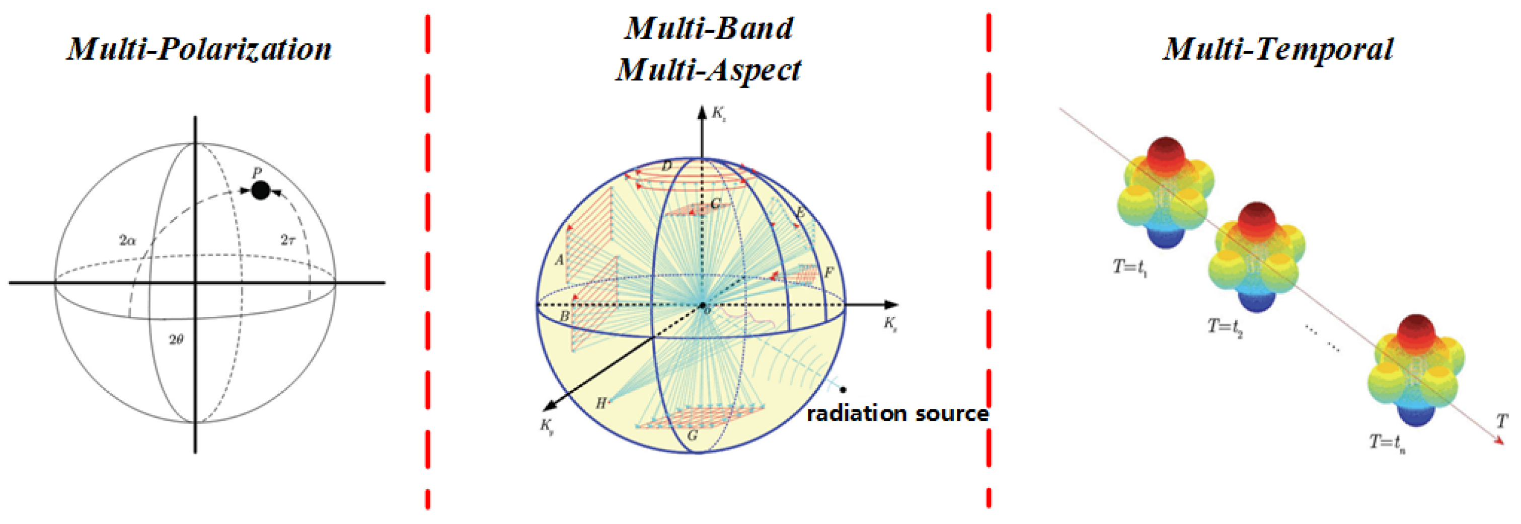
Figure 1.
Multi-dimensional electromagnetic scattering characteristics observation space concept diagram.
Figure 1.
Multi-dimensional electromagnetic scattering characteristics observation space concept diagram.
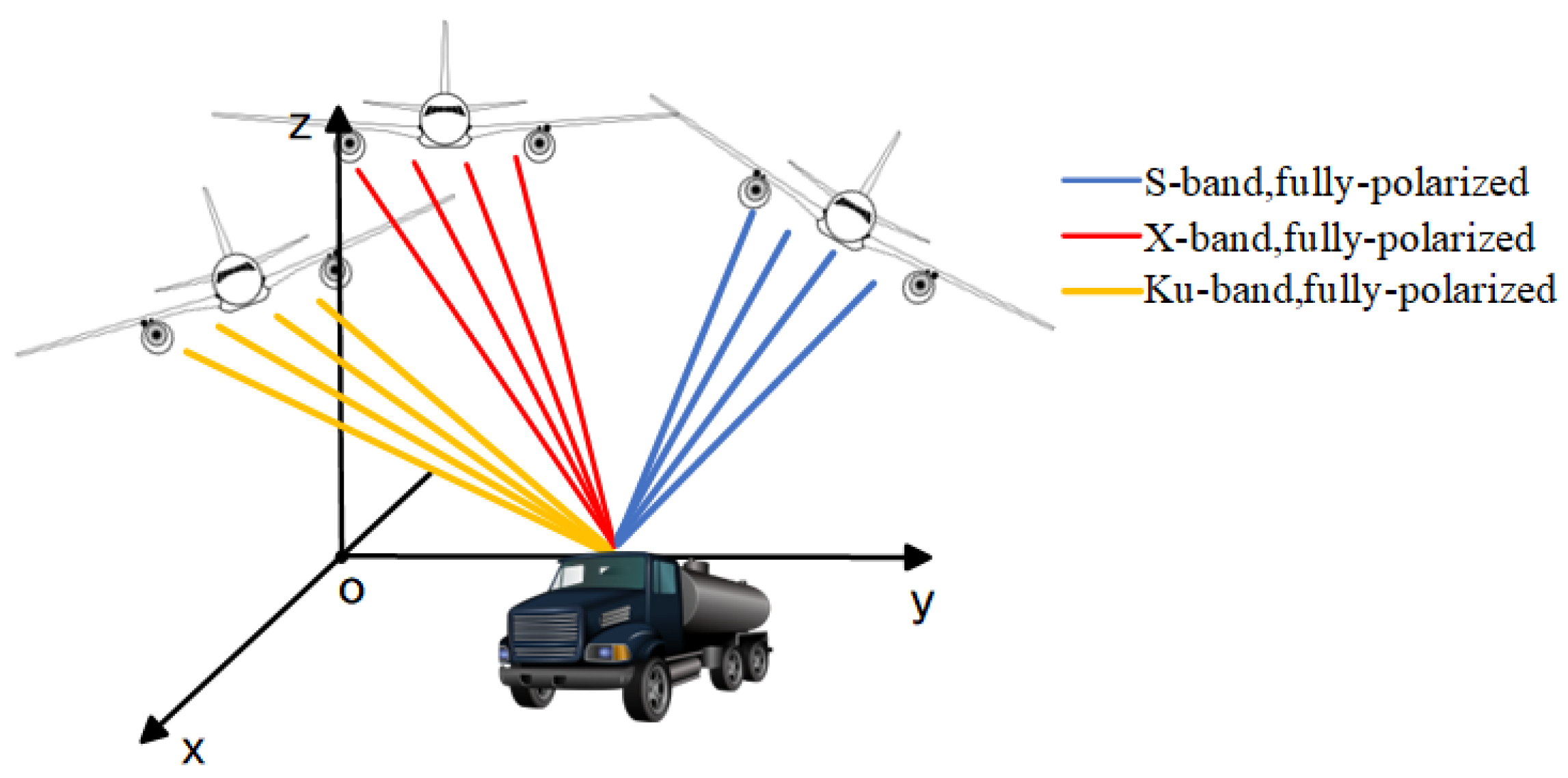
Figure 2.
Multi-dimensional electromagnetic scattering characteristics observation space concept diagram.
Figure 2.
Multi-dimensional electromagnetic scattering characteristics observation space concept diagram.
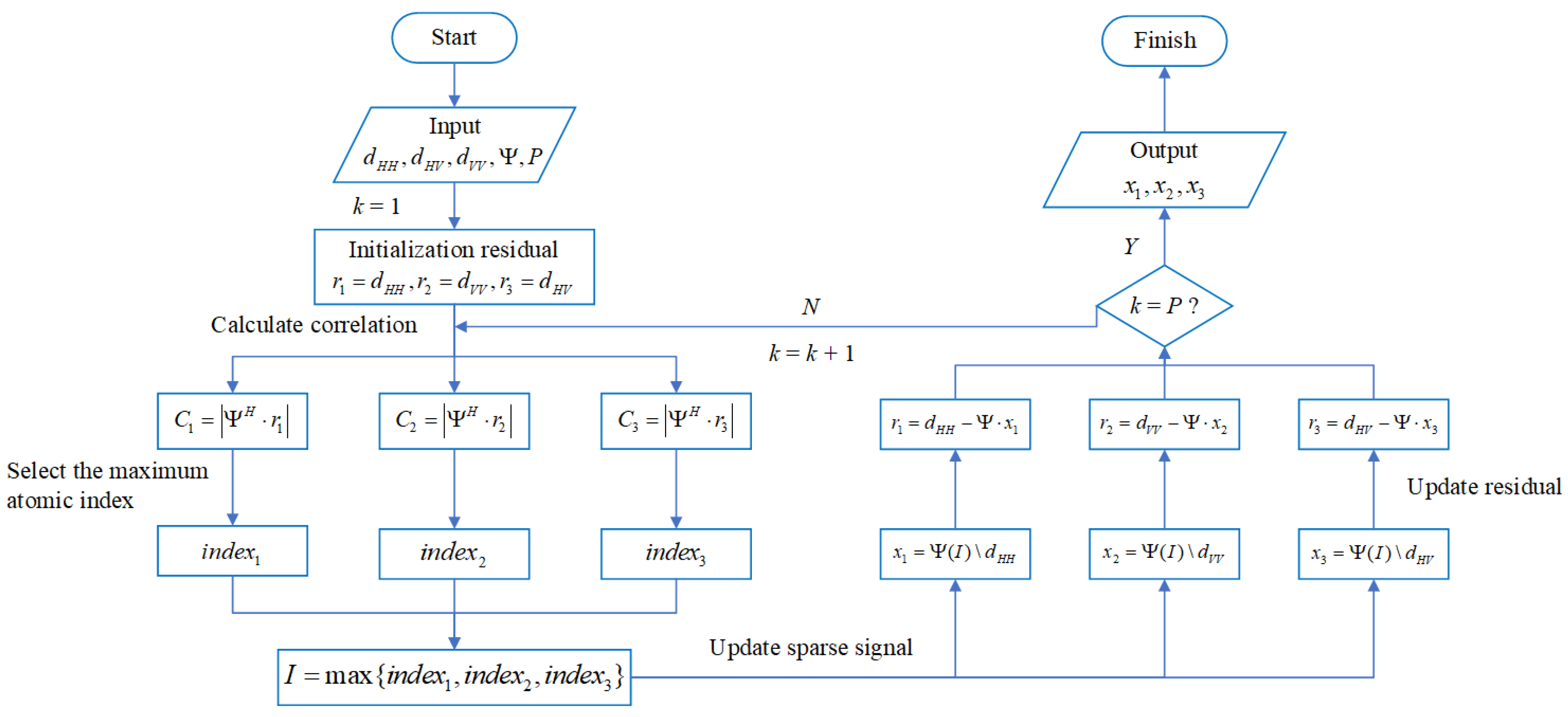
Figure 3.
Fully polarized ASC parameter optimization algorithm.
Figure 3.
Fully polarized ASC parameter optimization algorithm.
Figure 4.
Multi-angle polarization feature classification method based on sliding window Euclidean distance.
Figure 4.
Multi-angle polarization feature classification method based on sliding window Euclidean distance.
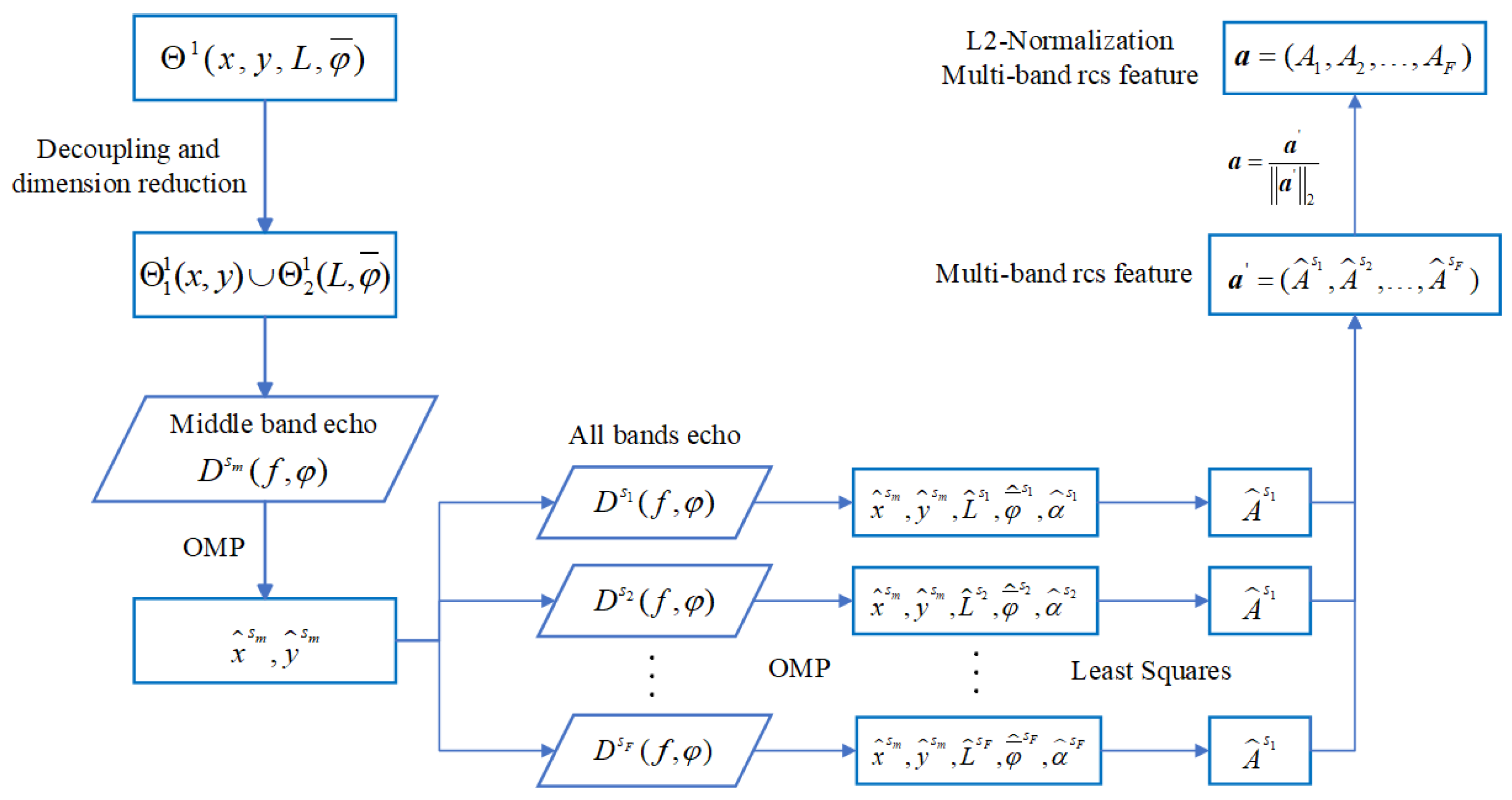
Figure 5.
Normalized multi-band joint rcs feature extraction flow chart.
Figure 5.
Normalized multi-band joint rcs feature extraction flow chart.
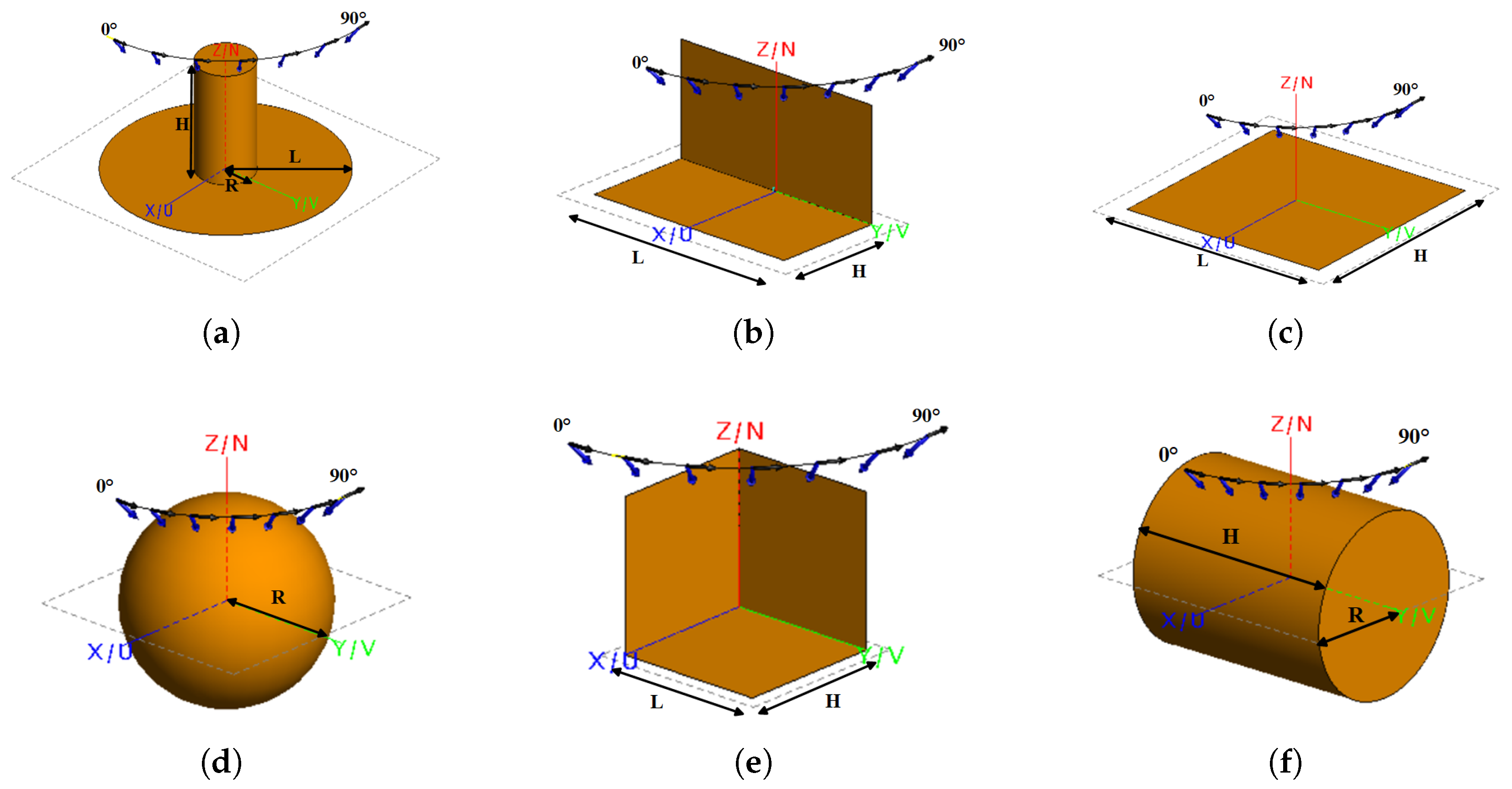
Figure 6.
Six typical scattering mechanisms of multi-angle full-polarization observation FEKO simulation scenarios and sizes (in meters as a unit): (a) Top hat, H = 0.15, R = 0.05, L = 0.2. (b) Dihedral, L = 1, H = 0.5. (c) Flatbed (edge diffraction), L = H = 0.5. (d) Sphere, R = 0.2. (e) Trihedral, L = H = 0.5. (f) Cylinder, H = 0.5 R = 0.2. The blue arrow represents the observation azimuth angle.
Figure 7.
The angular dimension expansion curves of multi-angle polarization characteristics of six typical scattering structures.
Figure 7.
The angular dimension expansion curves of multi-angle polarization characteristics of six typical scattering structures.
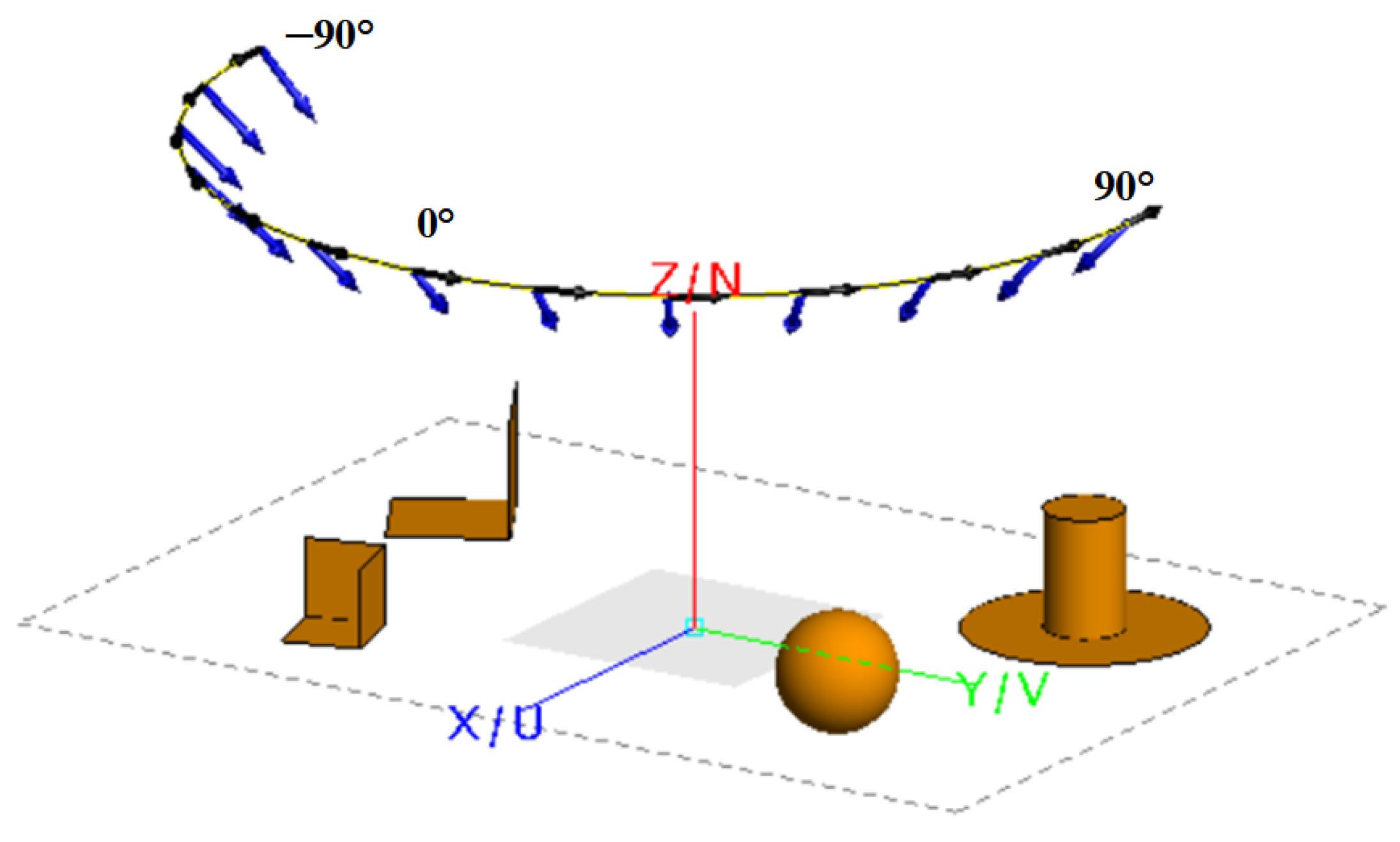
Figure 8.
FEKO electromagnetic simulation scenario with multiple scattering structures.The blue arrow represents the observation azimuth angle.
Figure 8.
FEKO electromagnetic simulation scenario with multiple scattering structures.The blue arrow represents the observation azimuth angle.
Figure 9.
Multi-angle imaging results of scene containing multiple scattering structures. The serial number represents the same scattering center corresponding to different angles.
Figure 9.
Multi-angle imaging results of scene containing multiple scattering structures. The serial number represents the same scattering center corresponding to different angles.
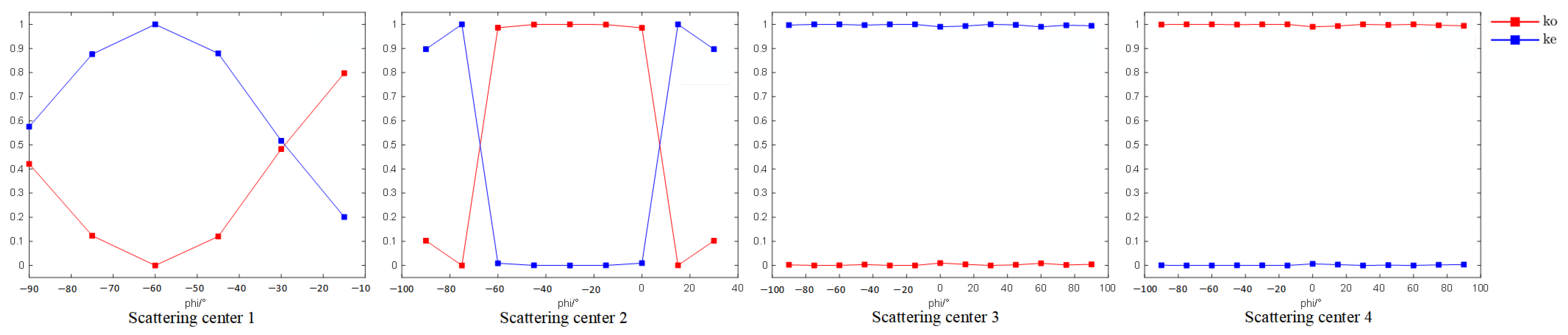
Figure 10.
Multi-angle polarization characteristic curves of four scattering centers in the multiple scattering structures experiment.
Figure 10.
Multi-angle polarization characteristic curves of four scattering centers in the multiple scattering structures experiment.
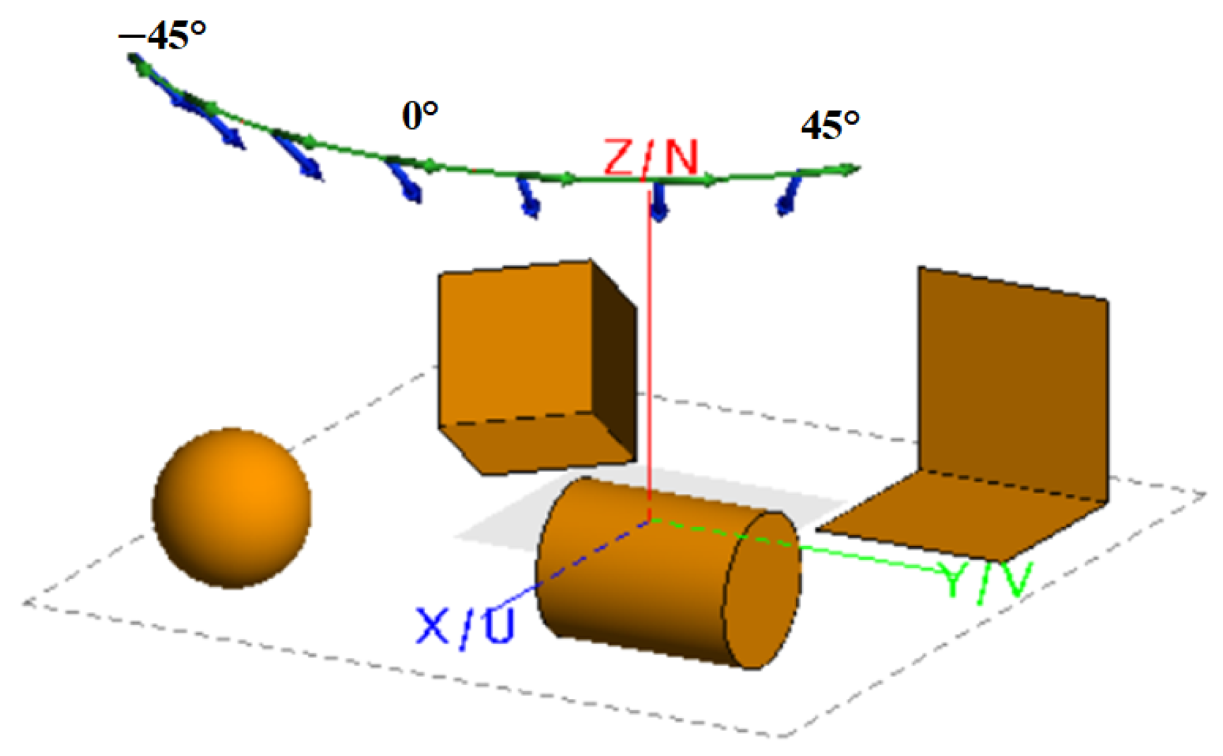
Figure 11.
Electromagnetic simulation scene of anti-noise experiment. The blue arrow indicates the azimuth angle of the observation.
Figure 11.
Electromagnetic simulation scene of anti-noise experiment. The blue arrow indicates the azimuth angle of the observation.
Figure 12.
Six typical scattering mechanisms multi-band observation FEKO simulation scenarios and sizes (in meters as a unit): (a) Top hat, H = 0.15, R = 0.05, L = 0.2. (b) Dihedral, L = 0.2, H = 0.2. (c) Flatbed (edge diffraction), L = H = 0.2. (d) Sphere, R = 0.2. (e) Trihedral, L = H = 0.2. (f) Cylinder, H = 0.3 R = 0.3.
Figure 13.
Normalized multi-band rcs characteristics of six typical scattering mechanisms.
Figure 13.
Normalized multi-band rcs characteristics of six typical scattering mechanisms.
Figure 14.
S, C, X, Ku, K five-band FDR matrix. Numbers 1, 2, 3, 4, 5, and 6 represent top hat, dihedral, plate, ball, trihedral, and cylinder, respectively. Red circles highlight the two categories with the smallest FDR.
Figure 14.
S, C, X, Ku, K five-band FDR matrix. Numbers 1, 2, 3, 4, 5, and 6 represent top hat, dihedral, plate, ball, trihedral, and cylinder, respectively. Red circles highlight the two categories with the smallest FDR.
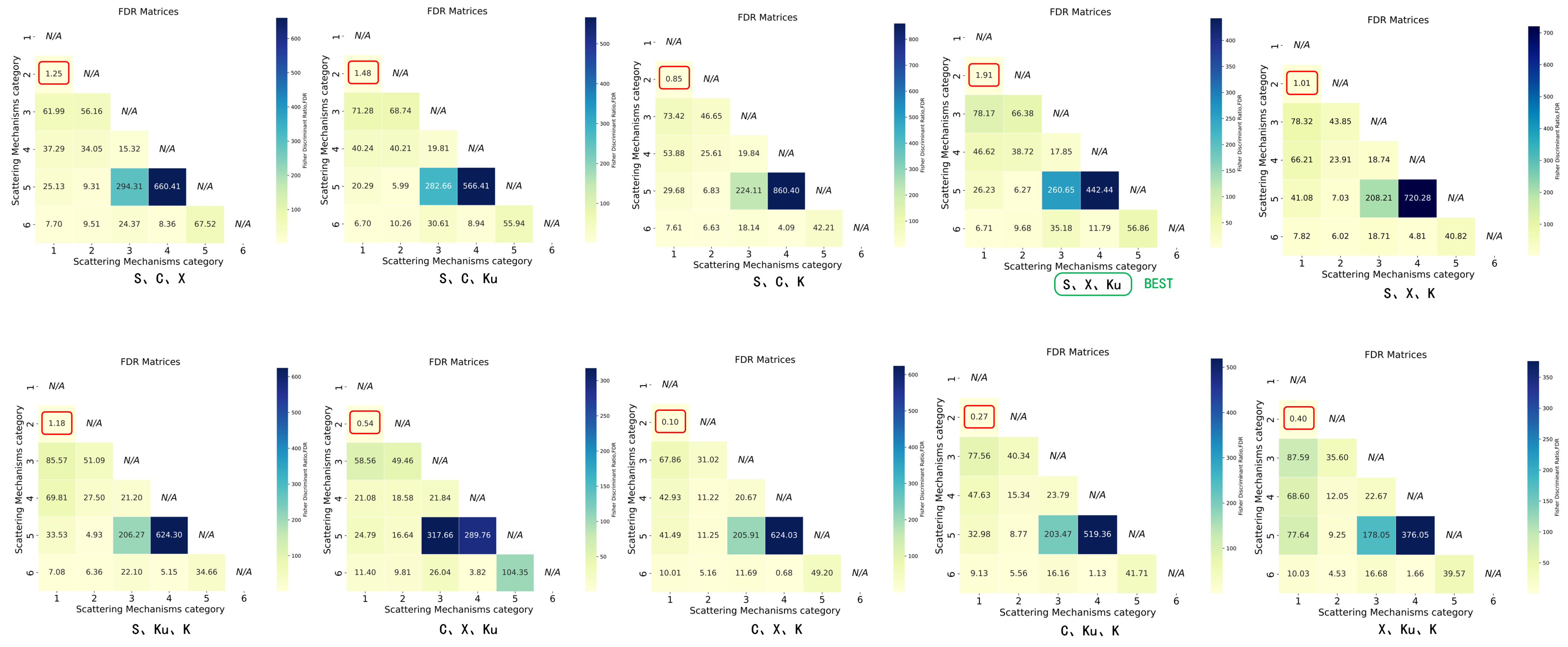
Figure 15.
The 4-band observation combination FDR matrices. Numbers 1, 2, 3, 4, 5, and 6 represent top hat, dihedral, plate, ball, trihedral, and cylinder, respectively. Red circles highlight the two categories with the smallest FDR. The green circle highlights the optimal observation combination.
Figure 15.
The 4-band observation combination FDR matrices. Numbers 1, 2, 3, 4, 5, and 6 represent top hat, dihedral, plate, ball, trihedral, and cylinder, respectively. Red circles highlight the two categories with the smallest FDR. The green circle highlights the optimal observation combination.
Figure 16.
The 3-band observation combination FDR matrices. Numbers 1, 2, 3, 4, 5, and 6 represent top hat, dihedral, plate, ball, trihedral, and cylinder, respectively. Red circles highlight the two categories with the smallest FDR. The green circle highlights the optimal observation combination.
Figure 16.
The 3-band observation combination FDR matrices. Numbers 1, 2, 3, 4, 5, and 6 represent top hat, dihedral, plate, ball, trihedral, and cylinder, respectively. Red circles highlight the two categories with the smallest FDR. The green circle highlights the optimal observation combination.
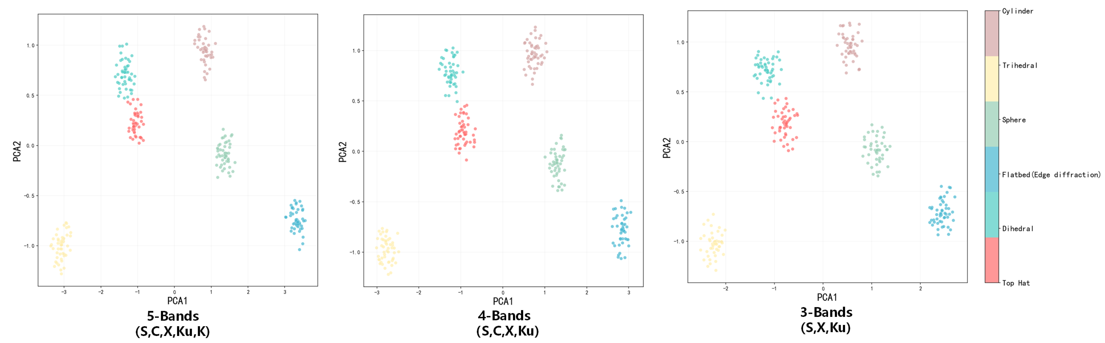
Figure 17.
Six scattering mechanisms frequency dimension separability visual point cloud diagram.
Figure 17.
Six scattering mechanisms frequency dimension separability visual point cloud diagram.
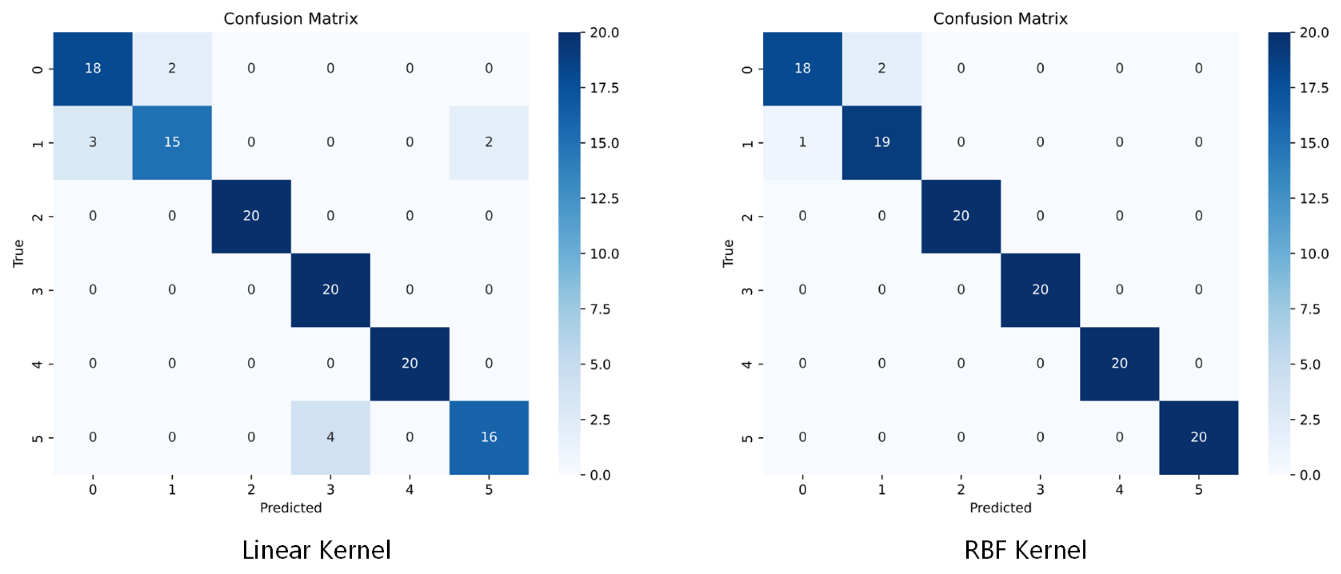
Figure 18.
The confusion matrix of linear kernel and RBF kernel classification on the test set under the combination of S, X, and Ku observations is used. Here, 0, 1, 2, 3, 4, and 5 represent the category top hat, dihedral, flat plate, ball, trihedral, and cylinder, respectively.
Figure 18.
The confusion matrix of linear kernel and RBF kernel classification on the test set under the combination of S, X, and Ku observations is used. Here, 0, 1, 2, 3, 4, and 5 represent the category top hat, dihedral, flat plate, ball, trihedral, and cylinder, respectively.
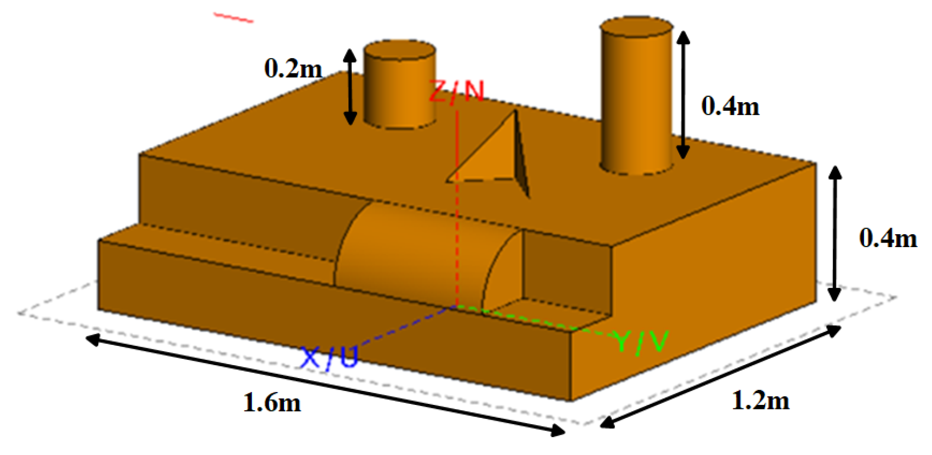
Figure 19.
Slicy model multi-band observation FEKO electromagnetic simulation scene.
Figure 19.
Slicy model multi-band observation FEKO electromagnetic simulation scene.
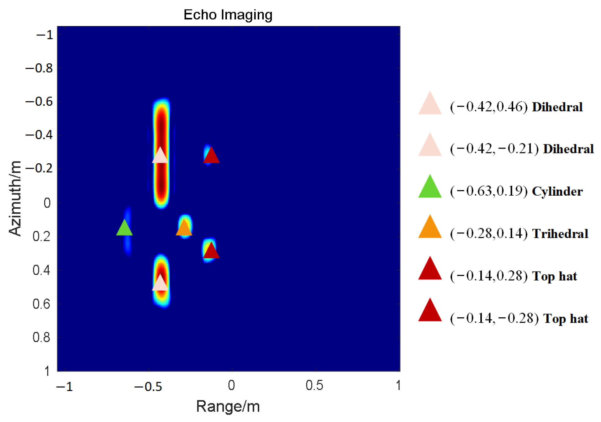
Figure 20.
Slicy model scattering center imaging classification results.
Figure 20.
Slicy model scattering center imaging classification results.
Figure 21.
Slicy model multi-angle full-polarization observation electromagnetic simulation scene. The blue arrow indicates the azimuth angle of the observation.
Figure 21.
Slicy model multi-angle full-polarization observation electromagnetic simulation scene. The blue arrow indicates the azimuth angle of the observation.
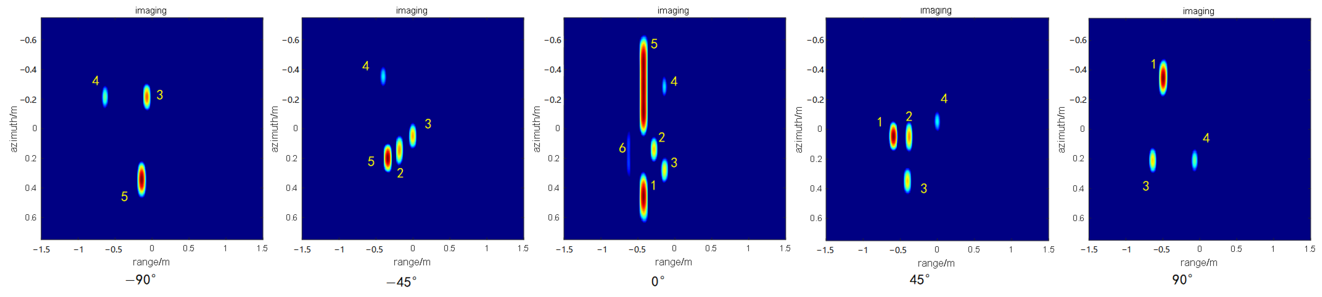
Figure 22.
Multi-angle observation imaging results of the Slicy model. The serial number represents the same scattering center corresponding to different angles.
Figure 22.
Multi-angle observation imaging results of the Slicy model. The serial number represents the same scattering center corresponding to different angles.
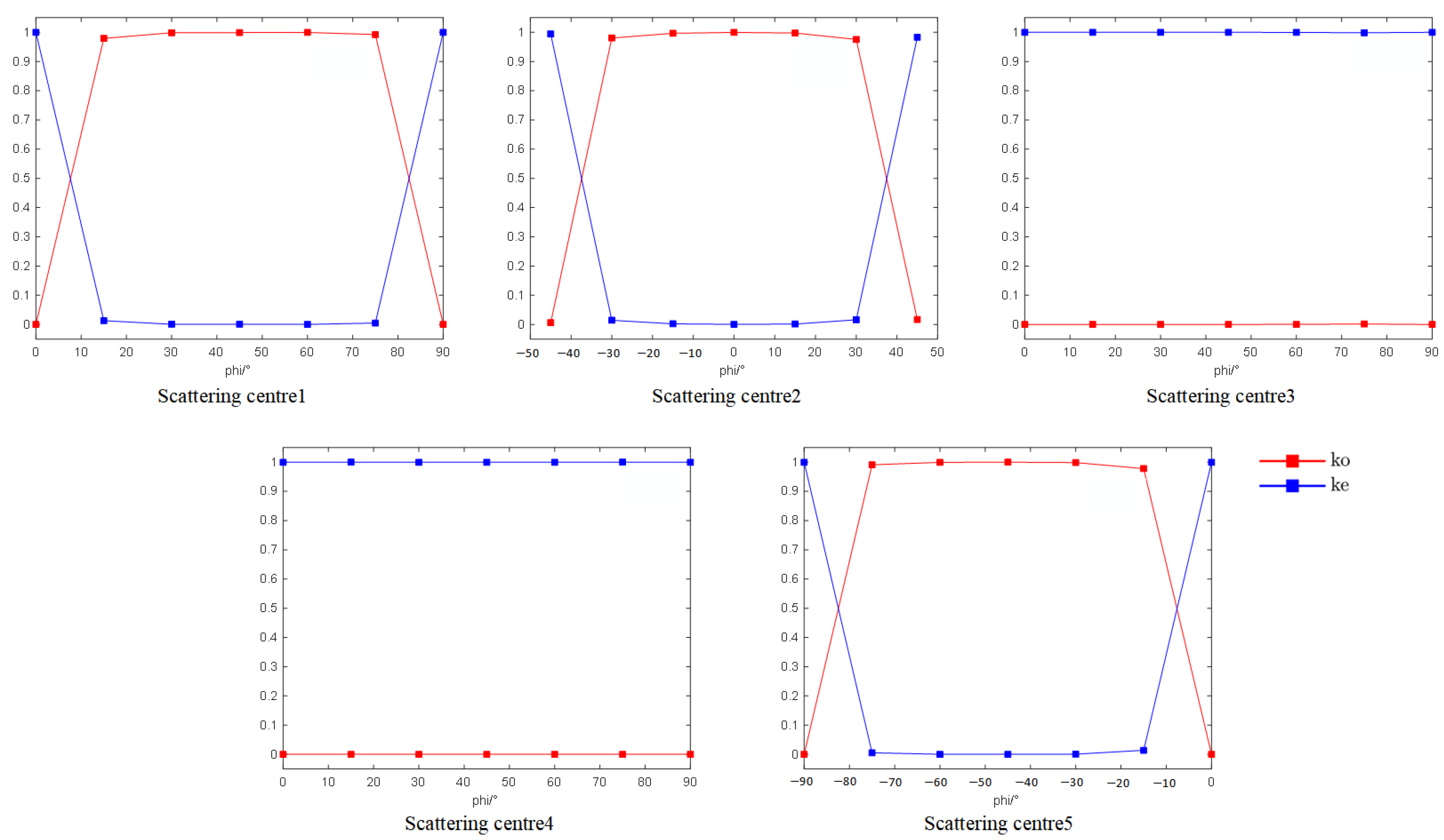
Figure 23.
Slicy model scattering center multi-angle Krogager decomposition polarization feature curve.
Figure 23.
Slicy model scattering center multi-angle Krogager decomposition polarization feature curve.
Table 1.
The scattering mechanism corresponding to different combinations of and L.
Table 1.
The scattering mechanism corresponding to different combinations of and L.
| Scattering Mechanism | | L | ASC Type |
|---|
| Dihedral | 1 | >0 | distributed |
| Trihedral | 1 | 0 | localized |
| Edge diffraction | −0.5 | >0 | distributed |
| Edge broadside | 0 | >0 | distributed |
| Sphere | 0 | 0 | localized |
| Top hat | 0.5 | 0 | localized |
| Cylinder | 0.5 | >0 | distributed |
| Corner diffraction | −1 | 0 | localized |
Table 2.
Typical scattering mechanism multi-angle full polarization observation simulation configuration.
Table 2.
Typical scattering mechanism multi-angle full polarization observation simulation configuration.
| Parameter | Value |
|---|
| Bandwidth | 1 GHz |
| Center frequency | 15 GHz |
| Beam width | |
| Down-looking angle | |
| Azimuth observation angle | , , , , , , |
| Polarization mode | HH, HV, VH, VV |
Table 3.
The main orientation of the scattering structure in the standard angular dimension space.
Table 3.
The main orientation of the scattering structure in the standard angular dimension space.
| Scattering Construction | Main Orientation |
|---|
| Dihedral | |
| Flatbed (edge diffraction) | , |
| Sphere | / |
| Trihedral | |
| Cylinder | |
| Top hat | / |
Table 4.
Scattering structure size and orientation setting.
Table 4.
Scattering structure size and orientation setting.
| Scattering Construction | Size | Main Orientation |
|---|
| Dihedral | L = H = 0.3 m | |
| Trihedral | L = H = 0.2 m | |
| Cylinder | H = 0.3 m, R = 0.1 m, L = 0.3 m | / |
| Top hat | R = 0.15 m | / |
Table 5.
Anti-noise experimental results. “✓” represents the number of correct recognition ≥45 times; “×” represents the number of correct recognition < 45 times.
Table 5.
Anti-noise experimental results. “✓” represents the number of correct recognition ≥45 times; “×” represents the number of correct recognition < 45 times.
| | 10 dB | 15 dB | 20 dB | 25 dB | 30 dB | 35 dB | 40 dB | 45 dB |
|---|
| | Single Angle ASC Parameter Estimation Classification |
| Dihedral | × | × | × | ✓ | ✓ | ✓ | ✓ | ✓ |
| Trihedral | × | × | × | × | × | ✓ | ✓ | ✓ |
| Sphere | × | × | × | × | × | × | ✓ | ✓ |
| Cylinder | × | × | × | × | × | × | ✓ | ✓ |
| | Multi-angle Krogager polarization decomposition feature classification method |
| Dihedral | × | × | × | ✓ | ✓ | ✓ | ✓ | ✓ |
| Trihedral | × | × | ✓ | ✓ | ✓ | ✓ | ✓ | ✓ |
| Sphere | × | × | × | × | ✓ | ✓ | ✓ | ✓ |
| Cylinder | × | × | × | × | × | ✓ | ✓ | ✓ |
Table 6.
Typical scattering mechanism multi-band observation simulation configuration.
Table 6.
Typical scattering mechanism multi-band observation simulation configuration.
| Parameter | Value |
|---|
| Bandwidth | 1 GHz |
| Center frequency | 3 GHz, 6 GHz, 9 GHz, 15 GHz, 20 GHz |
| Beam width | |
| Down-looking angle | |
| Azimuth observation angle | |
| Polarization mode | HH |
Table 7.
The recognition results of Slicy model scattering centers by traditional methods and multi-band feature extraction and classification methods. Pink filling indicates error recognition.
Table 7.
The recognition results of Slicy model scattering centers by traditional methods and multi-band feature extraction and classification methods. Pink filling indicates error recognition.
| Coordinates of Scattering Center | True Value | Conventional Method | 5-Band Classification S, C, X, Ku, K | 4-Band Classification S, C, X, Ku | 3-Band Classification S, X, Ku |
|---|
| −0.42, −0.21 | dihedral | dihedral | dihedral | dihedral | dihedral |
| −0.42, 0.46 | dihedral | dihedral | dihedral | dihedral | dihedral |
| −0.63, 0.19 | cylinder | dihedral | cylinder | cylinder | cylinder |
| −0.28, 0.14 | trihedral | trihedral | trihedral | trihedral | trihedral |
| −0.14, 0.28 | top hat | top hat | top hat | top hat | top hat |
| −0.14, −0.28 | top hat | dihedral | dihedral | top hat | top hat |
Table 8.
The recognition results of Slicy model scattering centers by 3-band different frequency observation combinations. Pink filling indicates error recognition. The number after frequency combination is its minimum FDR value.
Table 8.
The recognition results of Slicy model scattering centers by 3-band different frequency observation combinations. Pink filling indicates error recognition. The number after frequency combination is its minimum FDR value.
| Coordinates of Scattering Center | True Value | C, X, K (0.1) | S, C, K (0.85) | S, C, X (1.25) | S, X, Ku (Optimal) |
|---|
| −0.42, −0.21 | dihedral | dihedral | dihedral | dihedral | dihedral |
| −0.42, 0.46 | dihedral | dihedral | dihedral | dihedral | dihedral |
| −0.63, 0.19 | cylinder | sphere | cylinder | cylinder | cylinder |
| −0.28, 0.14 | trihedral | trihedral | trihedral | trihedral | trihedral |
| −0.14, 0.28 | top hat | dihedral | top hat | dihedral | top hat |
| −0.14, −0.28 | top hat | dihedral | dihedral | dihedral | top hat |
Table 9.
Multi-angle feature classification results of main scattering centers of Slicy model.
Table 9.
Multi-angle feature classification results of main scattering centers of Slicy model.
| Labels of Scattering Center | Classified Results | Orientation |
|---|
| 1 | trihedral | |
| 2 | trihedral | |
| 3 | top hat | / |
| 4 | top hat | / |
| 5 | trihedral | |


