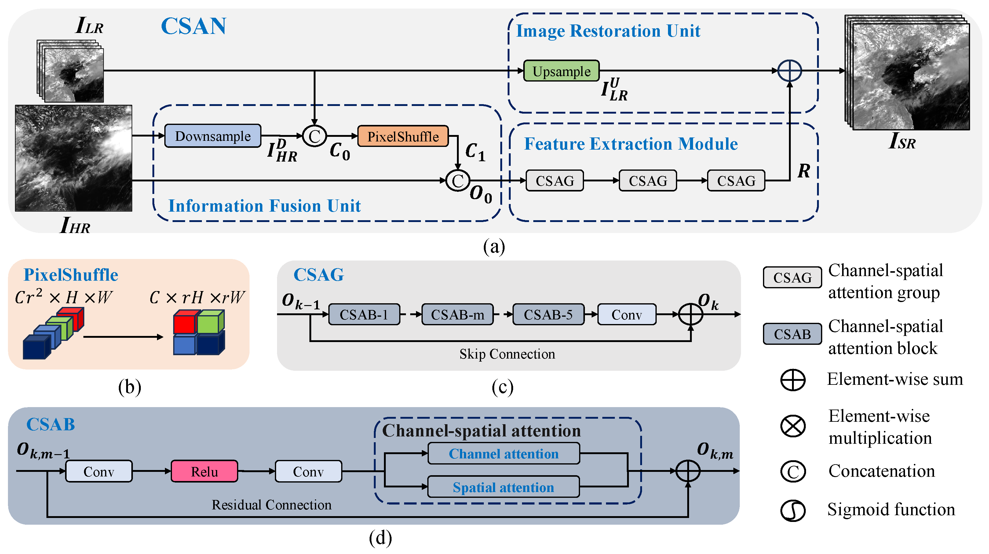
Figure 1.
Overall network structure of our proposed CSAN. (a) The architecture of CSAN, which consists of three parts: the information fusion unit, the feature extraction module, and the image restoration unit. represents the set of LR input bands, is the HR input, and is the super-resolved output. For the model, includes three 1 km bands and is the original 0.5 km band. For the model, includes twelve 2 km bands and combines the original 0.5 km band and the super-resolved 1 km bands. (b) Schematic diagram of the PixelShuffle module, which converts the channel dimension into the spatial dimension. (c) Illustration of the CSAG module, which includes five CSABs and a convolutional layer. (d) Illustration of the CSAB module containing the channel–spatial attention mechanism.
Figure 2.
Illustration of channel attention module and spatial attention module.
Figure 2.
Illustration of channel attention module and spatial attention module.
Figure 3.
Visual results of the SR for downsampled 1 km bands. To facilitate comparison, a false color composite is constructed using three bands: vi008 is mapped to red, vi005 to green, and vi004 to blue. Each panel shows the composite image formed by the super-resolved outputs of these three bands from the respective method.
Figure 4.
Average absolute error map between ground truth and SR result for all downsampled 1 km bands.
Figure 4.
Average absolute error map between ground truth and SR result for all downsampled 1 km bands.
Figure 5.
Visual results of the SR for downsampled 2 km bands. The first and second rows display images from the nr016 band with a central wavelength of 1.61 m, while the third and fourth rows display images from the ir105 band with a central wavelength of 10.403 m.
Figure 5.
Visual results of the SR for downsampled 2 km bands. The first and second rows display images from the nr016 band with a central wavelength of 1.61 m, while the third and fourth rows display images from the ir105 band with a central wavelength of 10.403 m.
Figure 6.
Average absolute error map between ground truth and SR result for all downsampled 2 km bands.
Figure 6.
Average absolute error map between ground truth and SR result for all downsampled 2 km bands.
Figure 7.
Visual results of CSAN and Bicubic on original 1 km GK2A satellite data, for the SR. Each row corresponds to a different testing region. From left to right, each column shows the original 0.5 km vi006 band (used as a reference), the original 1 km band (LR input), the result by Bicubic at 0.5 km resolution, and the result by CSAN at 0.5 km resolution.
Figure 8.
Visual results of CSAN and Bicubic on original 2 km GK2A satellite data, for the SR. Each row corresponds to a different test region. From left to right, each column shows the original 0.5 km vi006 band (used as a reference), the original 1 km band, the original 2 km band (LR input), the result for Bicubic at 0.5 km resolution, and the result for CSAN at 0.5 km resolution.
Table 1.
Specifications of sixteen GK2A bands.
Table 1.
Specifications of sixteen GK2A bands.
| Category | Band Number | Band Name | Center Wavelength [m] | Spatial Resolution [km] |
|---|
| Visible | 1 | vi004 | 0.47 | 1 |
| 2 | vi005 | 0.511 | 1 |
| 3 | vi006 | 0.64 | 0.5 |
| 4 | vi008 | 0.856 | 1 |
| Near-infrared | 5 | nr013 | 1.38 | 2 |
| 6 | nr016 | 1.61 | 2 |
| Short-wave infrared | 7 | sw038 | 3.83 | 2 |
| Water vapor | 8 | wv063 | 6.241 | 2 |
| 9 | wv069 | 6.952 | 2 |
| 10 | wv073 | 7.344 | 2 |
| Infrared | 11 | ir087 | 8.592 | 2 |
| 12 | ir096 | 9.625 | 2 |
| 13 | ir105 | 10.403 | 2 |
| 14 | ir112 | 11.212 | 2 |
| 15 | ir123 | 12.364 | 2 |
| 16 | ir133 | 13.31 | 2 |
Table 2.
Quantitative results of RMSE, PSNR, SRE, SAM, and ERGAS values for super-resolving downsampled 1 km bands. The metrics are averaged across all testing regions for the SR, evaluated at the lower scale (input resolution of 2 km, output resolution of 1 km). Arrows (↑/↓) indicate that higher/lower is better for the corresponding metric. The best results are indicated in bold.
| | vi004 | | vi005 | | vi008 | SAM↓ | ERGAS↓ |
|---|
|
RMSE↓
|
PSNR↑
|
SRE↑
|
RMSE↓
|
PSNR↑
|
SRE↑
|
RMSE↓
|
PSNR↑
|
SRE↑
|
|---|
| Bicubic | 32.58 | 35.37 | 27.62 | | 34.23 | 35.01 | 27.01 | | 151.62 | 34.39 | 26.94 | 0.35 | 2.25 |
| EDSR | 23.39 | 38.22 | 30.47 | | 24.11 | 38.06 | 30.06 | | 109.61 | 37.21 | 29.77 | 0.31 | 1.61 |
| SwinIR | 26.76 | 37.08 | 29.33 | | 28.14 | 36.72 | 28.73 | | 126.00 | 36.07 | 28.63 | 0.31 | 1.85 |
| Essaformer | 25.78 | 37.38 | 29.63 | | 27.41 | 36.93 | 28.93 | | 121.83 | 36.28 | 28.84 | 0.30 | 1.80 |
| DSen2 | 7.14 | 48.52 | 40.77 | | 7.50 | 48.17 | 40.17 | | 49.03 | 44.25 | 36.81 | 0.22 | 0.59 |
| Sen2-RDSR | 7.02 | 48.64 | 40.89 | | 7.20 | 48.51 | 40.52 | | 47.13 | 44.60 | 37.16 | 0.21 | 0.57 |
| PARNet | 7.37 | 48.24 | 40.50 | | 7.66 | 47.98 | 39.99 | | 50.39 | 44.02 | 36.57 | 0.22 | 0.60 |
| HFN | 7.12 | 48.55 | 40.80 | | 7.38 | 48.31 | 40.31 | | 49.10 | 44.25 | 36.80 | 0.22 | 0.59 |
| CSAN (Ours) | 6.17 | 49.75 | 42.00 | | 6.37 | 49.55 | 41.55 | | 44.77 | 45.07 | 37.62 | 0.19 | 0.52 |
Table 3.
Quantitative results of RMSE, PSNR, SRE, SAM, and ERGAS values for super-resolving downsampled 2 km bands. The metrics are averaged across all testing regions for the SR, evaluated at the lower scale (input resolution of 8 km, output resolution of 2 km). Arrows (↑/↓) indicate that higher/lower is better for the corresponding metric. The best results are indicated in bold.
| Metric | Bands | Bicubic | EDSR | SwinIR | Essaformer | DSen2 | Sen2-RDSR | PARNet | HFN | CSAN (Ours) |
|---|
| RMSE↓ | nr013 | 43.14 | 34.87 | 60.40 | 34.81 | 28.84 | 26.70 | 31.13 | 27.28 | 25.63 |
| nr016 | 41.24 | 38.74 | 51.37 | 38.84 | 21.52 | 20.80 | 23.20 | 21.22 | 20.17 |
| sw038 | 49.31 | 45.85 | 62.20 | 49.01 | 39.23 | 38.18 | 39.56 | 39.26 | 36.95 |
| wv063 | 4.74 | 9.31 | 6.38 | 7.47 | 3.55 | 3.55 | 3.53 | 3.86 | 3.40 |
| wv069 | 19.40 | 16.70 | 27.28 | 16.55 | 13.32 | 12.61 | 14.57 | 13.00 | 12.27 |
| wv073 | 33.22 | 26.06 | 47.99 | 26.89 | 21.28 | 20.02 | 22.85 | 20.67 | 19.68 |
| ir087 | 132.20 | 106.69 | 192.14 | 102.41 | 63.95 | 61.38 | 69.60 | 63.46 | 60.15 |
| ir096 | 70.05 | 58.88 | 101.56 | 54.77 | 34.60 | 32.94 | 41.42 | 34.24 | 32.56 |
| ir105 | 148.24 | 119.82 | 213.20 | 115.42 | 72.60 | 69.01 | 78.94 | 71.80 | 68.14 |
| ir112 | 141.40 | 113.82 | 204.82 | 109.23 | 71.51 | 67.94 | 77.69 | 71.75 | 67.12 |
| ir123 | 126.49 | 101.89 | 184.62 | 98.06 | 67.69 | 64.20 | 73.36 | 66.94 | 63.45 |
| ir133 | 85.54 | 68.22 | 122.54 | 66.36 | 49.39 | 46.81 | 53.30 | 48.79 | 46.07 |
| Mean | 74.58 | 61.74 | 106.21 | 59.99 | 40.62 | 38.64 | 44.00 | 40.10 | 37.98 |
| PSNR↑ | nr013 | 33.47 | 35.31 | 30.57 | 35.32 | 36.97 | 37.65 | 36.32 | 37.45 | 38.01 |
| nr016 | 27.76 | 28.30 | 25.85 | 28.28 | 33.52 | 33.82 | 32.84 | 33.63 | 34.09 |
| sw038 | 50.57 | 51.21 | 48.52 | 50.56 | 52.70 | 52.93 | 52.07 | 52.68 | 53.21 |
| wv063 | 58.88 | 52.71 | 56.32 | 54.78 | 61.24 | 61.26 | 60.43 | 60.42 | 61.60 |
| wv069 | 52.48 | 53.68 | 49.55 | 53.76 | 55.71 | 56.20 | 54.94 | 55.93 | 56.43 |
| wv073 | 47.67 | 49.75 | 44.50 | 49.48 | 51.52 | 52.07 | 50.93 | 51.79 | 52.22 |
| ir087 | 35.47 | 37.36 | 32.22 | 37.71 | 41.79 | 42.21 | 41.06 | 41.86 | 42.32 |
| ir096 | 40.57 | 42.06 | 37.36 | 42.70 | 46.71 | 47.15 | 46.03 | 46.80 | 47.24 |
| ir105 | 34.23 | 36.10 | 31.07 | 36.42 | 40.44 | 40.89 | 39.72 | 40.54 | 41.00 |
| ir112 | 34.52 | 36.44 | 31.30 | 36.79 | 40.44 | 40.89 | 39.73 | 40.54 | 41.01 |
| ir123 | 35.31 | 37.22 | 32.03 | 37.55 | 40.74 | 41.21 | 40.05 | 40.84 | 41.31 |
| ir133 | 38.52 | 40.48 | 35.41 | 40.73 | 43.32 | 43.79 | 42.67 | 43.42 | 43.90 |
| Mean | 40.79 | 41.72 | 37.89 | 42.01 | 45.43 | 45.83 | 43.99 | 45.44 | 46.03 |
| SRE↑ | nr013 | 16.90 | 18.74 | 14.00 | 18.75 | 20.40 | 21.07 | 19.74 | 20.88 | 21.44 |
| nr016 | 20.25 | 20.80 | 18.35 | 20.78 | 26.02 | 26.32 | 25.34 | 26.13 | 26.59 |
| sw038 | 50.30 | 50.94 | 48.25 | 50.29 | 52.42 | 52.66 | 51.80 | 52.40 | 52.94 |
| wv063 | 58.52 | 52.35 | 55.96 | 54.42 | 60.88 | 60.90 | 60.07 | 60.06 | 61.24 |
| wv069 | 51.81 | 53.01 | 48.88 | 53.10 | 55.04 | 55.53 | 54.28 | 55.26 | 55.76 |
| wv073 | 46.70 | 48.79 | 43.53 | 48.51 | 50.56 | 51.10 | 49.96 | 50.83 | 51.25 |
| ir087 | 33.00 | 34.88 | 29.74 | 35.23 | 39.31 | 39.73 | 38.58 | 39.38 | 39.85 |
| ir096 | 39.18 | 40.67 | 35.97 | 41.31 | 45.32 | 45.76 | 44.64 | 45.42 | 45.85 |
| ir105 | 31.10 | 32.98 | 27.95 | 33.29 | 37.32 | 37.76 | 36.60 | 37.42 | 37.87 |
| ir112 | 31.32 | 33.24 | 28.10 | 33.59 | 37.25 | 37.69 | 36.53 | 37.34 | 37.80 |
| ir123 | 32.13 | 34.04 | 28.85 | 34.37 | 37.56 | 38.02 | 36.87 | 37.66 | 38.13 |
| ir133 | 36.00 | 37.96 | 32.89 | 38.20 | 40.79 | 41.27 | 40.14 | 40.90 | 41.38 |
| Mean | 37.07 | 38.20 | 34.37 | 38.49 | 41.91 | 42.32 | 41.21 | 41.97 | 42.51 |
| SAM ↑ | | 0.41 | 0.35 | 0.57 | 0.35 | 0.23 | 0.22 | 0.25 | 0.23 | 0.21 |
| ERGAS ↓ | | 1.39 | 1.19 | 1.88 | 1.18 | 0.86 | 0.81 | 0.92 | 0.83 | 0.78 |
Table 4.
No-reference quality assessment for the SR on original 1 km bands, upsampled to 0.5 km resolution. NIQE, BRISQUE, and PIQE scores are computed for each band and then averaged across all bands and regions. Lower values indicate better perceptual quality. Arrows (↓) indicate that lower is better for the corresponding metric. The best results are highlighted in bold.
| Metric | Bicubic | EDSR | SwinIR | Essaformer | DSen2 | Sen2-RDSR | PARNet | HFN | CSAN (Ours) |
|---|
| NIQE↓ | 5.27 | 4.39 | 4.34 | 4.76 | 3.83 | 3.86 | 3.84 | 3.87 | 3.85 |
| BRISQUE↓ | 32.26 | 9.73 | 18.32 | 23.80 | 8.59 | 8.44 | 8.31 | 8.23 | 7.99 |
| PIQE↓ | 24.92 | 5.11 | 9.22 | 9.55 | 3.87 | 3.86 | 3.97 | 3.92 | 3.82 |
Table 5.
No-reference quality assessment for the SR on original 2 km bands, upsampled to 0.5 km resolution. NIQE, BRISQUE, and PIQE scores are computed for each band and then averaged across all bands and regions. Lower values indicate better perceptual quality. Arrows (↓) indicate that lower is better for the corresponding metric. The best results are highlighted in bold.
| Metric | Bicubic | EDSR | SwinIR | Essaformer | DSen2 | Sen2-RDSR | PARNet | HFN | CSAN (Ours) |
|---|
| NIQE↓ | 8.53 | 5.11 | 5.11 | 5.61 | 4.34 | 4.43 | 4.58 | 4.45 | 4.52 |
| BRISQUE↓ | 46.78 | 27.46 | 21.74 | 56.76 | 10.15 | 8.27 | 11.91 | 9.19 | 7.93 |
| PIQE↓ | 58.02 | 26.56 | 17.13 | 16.59 | 13.91 | 14.20 | 15.89 | 14.34 | 13.77 |
Table 6.
Results of the ablation study for the SR. Arrows (↑/↓) indicate that higher/lower is better for the corresponding metric. The best results are indicated in bold.
Table 6.
Results of the ablation study for the SR. Arrows (↑/↓) indicate that higher/lower is better for the corresponding metric. The best results are indicated in bold.
| Model Variant | RMSE↓ | PSNR↑ | SRE↑ | SAM ↓ | ERGAS↓ |
|---|
| w/o-IFU | 20.02 | 47.86 | 39.93 | 0.1991 | 0.5450 |
| w/o-CA | 19.64 | 47.91 | 40.08 | 0.2013 | 0.5614 |
| w/o-SA | 19.95 | 47.76 | 39.85 | 0.1960 | 0.5386 |
| CSAN | 19.10 | 48.12 | 40.40 | 0.1938 | 0.5219 |
Table 7.
Results of the ablation study for the SR. Arrows (↑/↓) indicate that higher/lower is better for the corresponding metric. The best results are indicated in bold.
Table 7.
Results of the ablation study for the SR. Arrows (↑/↓) indicate that higher/lower is better for the corresponding metric. The best results are indicated in bold.
| Model Variant | RMSE↓ | PSNR↑ | SRE↑ | SAM ↓ | ERGAS↓ |
|---|
| w/o-IFU | 38.81 | 45.79 | 42.26 | 0.2241 | 0.7905 |
| w/o-CA | 39.29 | 45.70 | 42.18 | 0.2304 | 0.8099 |
| w/o-SA | 39.64 | 45.58 | 42.07 | 0.2249 | 0.7968 |
| CSAN | 37.98 | 46.03 | 42.51 | 0.2192 | 0.7782 |
Table 8.
Complexity comparison of methods in terms of parameters, training, and inference time for super-resolving 1 km bands.
Table 8.
Complexity comparison of methods in terms of parameters, training, and inference time for super-resolving 1 km bands.
| | EDSR | SwinIR | Essaformer | DSen2 | Sen2-RDSR | PARNet | HFN | CSAN (Ours) |
|---|
| Parameters (K) | 2403 | 1394 | 2144 | 1779 | 2162 | 833 | 1620 | 1268 |
| Training Time (h) | 9.80 | 44.36 | 6.84 | 4.08 | 9.99 | 4.88 | 8.64 | 5.45 |
| Inference Time (s) | 6.90 | 39.17 | 9.09 | 6.03 | 10.8 7 | 5.20 | 11.06 | 5.21 |
Table 9.
Complexity comparison of methods in terms of parameters, training, and inference time for super-resolving 2 km bands.
Table 9.
Complexity comparison of methods in terms of parameters, training, and inference time for super-resolving 2 km bands.
| | EDSR | SwinIR | Essaformer | DSen2 | Sen2-RDSR | PARNet | HFN | CSAN (Ours) |
|---|
| Parameters (K) | 2414 | 1409 | 2792 | 1803 | 2174 | 845 | 1665 | 1280 |
| Training Time (h) | 14.00 | 56.95 | 17.29 | 6.94 | 15.76 | 6.23 | 17.79 | 8.46 |
| Inference Time (s) | 6.40 | 36.43 | 9.15 | 5.85 | 8.08 | 5.59 | 8.13 | 5.58 |


