Classification of Precipitation Types and Investigation of Their Physical Characteristics Using Three-Dimensional S-Band Dual-Polarization Radar Data

Abstract

A novel classification algorithm for precipitation types (CP) was developed to address frequent misclassification issues between shallow convection and intense stratiform precipitation using existing methods and to enhance an understanding of their physical characteristics. Based on three-dimensional radar data and temperature fields, CP integrates three approaches: Storm Labeling in Three Dimensions (SLTD), a feature parameter-based algorithm (FP), and an advanced subcategorization method. The algorithm classifies precipitation into ten types: four non-precipitating, three stratiform, and three convective categories. CP was evaluated against traditional methods (SHY and FP) through both qualitative and quantitative analyses for mid-latitude warm-season systems. The CP method demonstrated improved performance, with higher skill scores (e.g., POD: 0.567–0.571) compared to SHY (0.349–0.364) and FP (0.455–0.470). Additionally, comparative analyses of vertical mean profiles of radar reflectivity, dynamical, and microphysical variables confirmed the enhanced capability of CP in distinguishing detailed precipitation structures.

1. Introduction

Stratiform and convective precipitation develop through distinct mechanisms, resulting in different cloud structures. Starzec et al. [1] described the differences between these precipitation types in terms of (1) microphysical composition, (2) thermodynamic properties, and (3) their relative frequency of occurrence across the globe. The Korean Peninsula, characterized by complex topography and surrounded by the sea, experiences various storm types caused by thermodynamic convection, moist southwesterly flows, and interactions between continental and marine air masses. Lee and Kim [2] identified four types of heavy precipitation systems (HPS)—isolated thunderstorms, convective bands, cloud clusters, and squall lines—based on satellite, ground radar, radiosonde, and automated weather station (AWS) data. However, their classification was largely phenomenological and limited in resolving the vertical structure of stratiform and convective regions.

Since 2014, the radar networks at the Weather Radar Center (WRC) of the Korea Meteorological Administration (KMA) have been upgraded to S-band dual-polarization radars. These radars provide microphysical variables such as reflectivity (Z_H), differential reflectivity (Z_DR), specific differential phase (K_DP), and cross-correlation coefficient (ρ_HV), which are less affected by attenuation. These variables enable more accurate identification of hydrometeor types and convective structures, including strong updrafts. Classification of precipitation types helps improve the understanding of the dynamic and microphysical characteristics of precipitation systems in mid-latitude environments, such as the Korean Peninsula, thereby enhancing precipitation estimation and insights into severe weather development.

Several earlier studies developed classification algorithms using radar reflectivity (Z_H) to distinguish between stratiform and convective precipitation [3,4,5,6,7]. Steiner et al. [4] proposed a method—hereafter referred to as SHY—that classifies convective and stratiform regions using Z_H at a constant altitude (e.g., 3 km), based on a reflectivity threshold known as peakedness. Peakedness is defined as the difference between the reflectivity at a grid point and the mean (or median) reflectivity within an 11 km radius. Powell et al. [7] supplemented SHY with a polar coordinate algorithm using single-radar low-elevation observations to improve precipitation estimation. However, these methods often misclassify weak or shallow convection and intense stratiform precipitation due to reliance on low-altitude, single-radar thresholds. This hinders detailed analysis of vertical precipitation structures, such as precipitation particle growth and the relationship between ice fluxes and lightning in updraft regions [8,9]. Fabry and Zawadzki [3] analyzed precipitation system organization using vertical reflectivity profiles from an X-band vertically pointing radar; however, their approach lacked sufficient spatial coverage to effectively analyze precipitation type distributions.

Some studies combined disdrometer and radar data to classify precipitation types [10,11,12]. Bringi et al. [10] utilized radar-derived microphysical parameters, including the generalized intercept parameter (N_w) and mass-weighted mean diameter (D_m), assuming a gamma drop size distribution (DSD), to distinguish between convective and stratiform regions. Their results showed convective points clustering above a linear fit line, representing the relationship between mean log (N_w) and D_m in stratiform regions. However, these parameters are sensitive to the shape parameter μ of the DSD, and their validation remains challenging. Loh et al. [12] applied a fuzzy logic method using single dual-polarization radar data in central South Korea, revealing DSD differences between stratiform and convective regions. While effective, this method had a limited spatial scope and primarily supported convection/stratiform classification.

To overcome these limitations, several classification schemes using three-dimensional (3D) radar observations have been proposed [1,13,14]. Feng et al. [13] developed a hybrid classification algorithm (HCA) that combines 3D radar reflectivity with GOES satellite products, including infrared brightness temperature and retrieved cloud top and base heights. However, this method relies on the availability of both radar and satellite data and is affected by smoothing artifacts resulting from horizontal resolution merging. Starzec et al. [1] introduced the Storm Labeling in Three Dimensions (SLTD) approach using dual-polarization radar to effectively identify updraft regions based on thresholds of Z_H, Z_DR, and K_DP. Dixon and Romatschke [14] proposed the Echo Classification from Convectivity (ECCO) algorithm, which uses reflectivity texture and convectivity from 3D radar networks and temperature fields. Despite such advances, accurately distinguishing deep stratiform systems remains a challenge.

In this study, we developed a new classification algorithm for precipitation types (CP) using 3D observational data from dense ground-based radar networks and atmospheric temperature fields. The CP algorithm integrates three components: (1) the SLTD method, (2) the feature parameter-based classification algorithm (FP), and (3) the advanced subcategorization method (ASM). SLTD enables classification of non-precipitating areas, stratiform, convective, and updraft regions by analyzing vertical radar structures. The FP method identifies deeply developed stratiform systems based on upper-level reflectivity features. ASM classifies shallow convection and stratiform regions with embedded bright bands using echo top height (ETH) and column-maximum reflectivity (CMAXZ). This integrated approach leverages the strengths of each method while addressing the known limitations in distinguishing between shallow convection and intense stratiform precipitation. The following sections detail the radar and temperature datasets (Section 2), CP algorithm and precipitation type analysis (Section 3), classification results and comparative evaluation (Section 4), and discussion and conclusions (Section 5 and Section 6).

2. Data

The radar-based 3D (R3D) Constant Altitude Plan Position Indicator (CAPPI) datasets of reflectivity (Z_H), differential reflectivity (Z_DR), specific differential phase (K_DP), and cross-correlation coefficient (ρ_HV) were provided by the Weather Radar Center (WRC) of the Korea Meteorological Administration (KMA). The radar network was manufactured by Enterprise Electronics Corporation (Enterprise, AL, USA). These datasets were collected during 20 rainfall events (

Table 1. A summary of selected rainfall cases and their characteristics.

No.	Selected Time [UTC]	Precipitation Types	Duration [hours]
1	17 May 2019. 20:00	Mid-latitude cyclone	22
2	26 May 2019. 23:30	Mid-latitude cyclone	34
3	6 June 2019. 11:30	Mid-latitude cyclone	29
4	26 June 2019.03:00	Mid-latitude cyclone	37
5	29 June 2019. 08:30	Changma front	20
6	10 July 2019. 06:00	Mid-latitude cyclone	27
7	21 August 2019. 23:30	Parallel squall line	24
8	26 August 2019. 23:00	Mid-latitude cyclone	20
9	2 September 2019. 00:00	Parallel squall line	12
10	2 September 2019. 21:30	Parallel squall line	13
11	18 May 2020. 08:00	Diagonal squall line related in cold front	23
12	24 June 2020. 01:30	Mid-latitude cyclone	30
13	29 June 2020. 13:00	Mid-latitude cyclone	47
14	10 July 2020. 01:00	Mid-latitude cyclone	30
15	12 July 2020. 21:30	Mid-latitude cyclone	42
16	13 July 2020. 14:30	Mid-latitude cyclone	14
17	28 July 2020. 23:30	Parallel squall line	11
18	2 August 2020. 06:30	Diagonal squall line	11
19	2 August 2020. 17:00	Parallel squall line	11
20	5 August 2020. 17:00	Mid-latitude cyclone	16

) that occurred in the warm seasons (May to September) of 2019 and 2020. To evaluate the classification capability of the CP algorithm and analyze the physical characteristics of various precipitation types, representative cases were deliberately selected. The time points listed in Table 1 correspond to snapshots when heavy rainfall occurred over the Korean Peninsula, typically associated with widespread precipitation systems embedded with convective bands. These include mid-latitude cyclones, the Changma front, and squall lines or convective bands, which are commonly observed in this region. The R3D CAPPI datasets incorporate dual-polarization observations from 11 S-band radars, offering high spatiotemporal resolution (Figure 1). Each dataset includes 200 vertical layers, covering altitudes from 50 m to 10 km. The temporal resolution is 5 min, with horizontal and vertical resolutions of 500 m and 50 m, respectively.

The melting layer plays a key role in distinguishing different precipitation types. In this study, the melting layer was identified using three-dimensional temperature fields, including air temperature (T), dew point temperature (T_d), and wet-bulb temperature (T_w). These temperature fields were generated using multi-quadric interpolation, based on data from the Very Short-Range Data Assimilation and Prediction System (VDAPS) and additional observational sources [15]. The temperature fields have a temporal resolution of 5 min and a horizontal resolution of 4 km. Vertically, they consist of 61 layers, with a resolution of 0.1 km below 2 km and 0.2 km above 2 km.

Dynamic variables, including the three-dimensional wind components (u, v, w), relative vorticity, and divergence (or convergence), were derived using the Wind Synthesis System using Doppler Measurements (WISSDOM) to analyze the dynamic characteristics of various precipitation systems. WISSDOM is a variational analysis method designed to produce realistic 3D wind fields by incorporating multiple observational datasets and background fields from numerical models [16,17]. Input data for WISSDOM included wind measurements from AWSs, as well as three-dimensional radar grid data of reflectivity (Z_H, in dBZ) and radial velocity (V_r, in m s⁻¹) from individual KMA operational radar sites, based on the CAPPI method. The terminal velocity of hydrometeors was calculated using air density and temperature profiles obtained from radiosonde observations. The background wind fields were taken from the Local Data Assimilation and Prediction System (LDAPS), which has a spatial resolution of 1.5 km and a temporal resolution of 3 h. The WISSDOM algorithm uses a variational optimization technique to minimize the following cost function:

$$J=\sum _{M=1}^5{J}_M$$

(1)

Each term represents a constraint, including: (1) the geometric relationship between radial velocity (V_r) from multiple radar sites and the Cartesian wind components, (2) the difference between the retrieved wind fields and background winds, (3) the anelastic continuity equation, (4) the vertical vorticity equation, and (5) a Laplacian smoothing constraint. These constraints are described in detail by Tsai et al. [17]. The WISSDOM analysis domain spans from 32.64° to 39.14°N in latitude and from 123.17° to 130.73°E in longitude, as indicated by the rectangular box in Figure 1. The output wind fields are provided on a 701 × 701 horizontal grid with a spatial resolution of 1 km × 1 km and a vertical resolution of 0.25 km, covering altitudes from 0 to 10 km across 41 layers. The temporal resolution of the WISSDOM output is 10 min.

Due to noise contamination, unrealistic vertical velocity (w-component) values of WISSDOM exceeding 15.0 m s⁻¹ were removed, regardless of height and precipitation type. Jorgensen and LeMone [18] investigated vertical velocity characteristics of both updrafts and downdrafts in oceanic convection near Taiwan. In their study, stronger 10%-level values of the mean and maximum vertical velocities in the updraft regions were approximately 2 and 3 m s⁻¹ at 300 m, and 6 and 9 m s⁻¹ at 6 km altitude, respectively. Considering the general characteristics of vertical wind components (u, v, w), observational artifacts were further eliminated using quality control (QC) procedures recommended by the World Meteorological Organization (WMO) [19].

Figure 2 illustrates the QC procedure, which consists of two stages: a domain test and a tracking test applied to wind observations. The domain test assesses whether wind component values fall within physically plausible limits and removes outliers based on predefined minimum and maximum thresholds. The tracking test consists of three steps—horizontal variation, horizontal blob, and vertical variation tests—to assess the spatial and vertical consistency of wind observations among neighboring grid points. The horizontal variation test detects spatial inconsistencies by calculating the standard deviation (σ) within a 5 × 5 grid window. The horizontal blob test identifies isolated anomalies using the median and the median absolute deviation (MAD), defined as:

$$MAD=median\left(\left|x\left(i,j,k\right)-median\left(x\right)\right|\right)$$

(2)

where x represents the wind component, and i, j, and k denote the longitude, latitude, and vertical indices, respectively. The vertical variation test evaluates gradients between adjacent layers to detect outliers in the vertical direction.

Table 2. Threshold values used in the quality control procedures for the 3D wind components based on WISSDOM.

	Proxy x	${\mathit{u}}_{\mathit{t}\mathit{h}\mathit{r}}$ [m s−1]	${\mathit{v}}_{\mathit{t}\mathit{h}\mathit{r}}$ [m s−1]	${\mathit{w}}_{\mathit{t}\mathit{h}\mathit{r}}$ [m s−1]
Test Types
Domain test		(minimum) −100 (maximum) 100	(minimum) −100 (maximum) 100	(minimum) −14 (maximum) 14
Horizontal variation test		100	100	3
Vertical variation test		30	30	14

summarizes the threshold values applied in each QC test. The QC algorithm was applied to a total of 349,324,380 grid samples across the 20 rainfall cases listed in Table 1. Figure 3 shows the Contoured Frequency by Altitude Diagram (CFAD) of the vertical wind component (w) in updraft regions, as discussed in Section 3.1. As shown in Figure 3a, extreme outliers reaching up to 15.0 m s⁻¹ were clearly identified and effectively removed through the QC process, resulting in a much cleaner and more realistic distribution in Figure 3b.

The spatial resolutions and vertical layer structures differed among the 3D datasets used in this study, including the R3D CAPPI, temperature fields, and WISSDOM outputs. To facilitate the analysis of the dynamic and microphysical characteristics of different precipitation types, all datasets were interpolated to a standard grid with a horizontal resolution of 1.0 km, vertical resolution of 0.25 km, and 40 vertical layers. Although the temperature fields and WISSDOM outputs were resampled to match the resolution of the 3D CAPPI data, this interpolation process may introduce smoothing effects or artificial detail, particularly in regions with strong spatial gradients. For example, the vertical precision of the melting layer height derived from the original 4 km resolution temperature fields may be limited after interpolation. Similarly, fine-scale structures in vertical velocity fields from WISSDOM may appear more detailed than the native resolution would support. To address these issues, the melting layer height was estimated with care, taking into account the resolution limitations of the interpolated temperature data. In addition, quality control (QC) procedures were applied to the WISSDOM-derived wind components to remove unrealistic values and minimize the risk of overinterpreting artificially enhanced small-scale features.

Additionally, long-term raindrop size distribution (RSD, N(D); m⁻³ mm⁻¹) datasets were obtained from a two-dimensional video disdrometer (2 DVD) to derive polynomial regression relationships between microphysical parameters and dual-polarization radar variables, as described in Section 3.2. The 2 DVD was manufactured by JOANNEUM RESEARCH, based in Graz, Austria. Summer season rainfall data from various 2 DVD sites were used in this study, including Daegu (2011–2012), Boseong (2013–2015, 2018–2019), Daegwallyeong (2017–2018), Incheon (2020), and Jinchun (2016–2018). The 2 DVD is a high-performance optical disdrometer that provides physical characteristics of precipitation particles by capturing their silhouettes using two orthogonally arranged line-scan cameras. Detailed specifications and data products of the 2 DVD are described in Bang et al. [20]. In brief, the RSD is defined as follows:

$$N\left(D_i\right)=\sum _{j=1}^n{\displaystyle \frac{1}{A_j{V}_{f,j}∆t∆D}},$$

(3)

where the subscript i denotes the diameter bin number (total 41 bins from 0.125 mm to 10.25 mm), and n is the total number of drops observed within a one-minute interval. V_f (m s⁻¹) and A_j represent the terminal fall velocity and the sampling area for each drop, respectively. ∆D and ∆t are fixed at 0.25 mm and 1 min. The QC process for 2 DVD data consists of two main steps. First, outliers were removed based on fall velocity using the method proposed by Kruger and Krajewski [21], defined as:

$$\left|V_a\left(D\right)-V_f\left(D\right)\right|<0.4V_a\left(D\right).$$

(4)

where V_a(D) = 9.65 − 10.3 exp(−0.6D), as given by Atlas et al. [22]. After this filtering step, the RSD was recalculated using Equation (3). A continuity test was then applied to ensure the physical plausibility of the RSD, following the method suggested by Bang et al. [20] and others [23,24,25], as the RSD is generally assumed to follow a continuous function.

3. Methodology

3.1. Description of Classification Algorithm for Precipitation Types (CP)

As described earlier, the newly developed CP algorithm for precipitation classification is composed of three modules: SLTD, FP, and ASM. The algorithm was executed on a Linux platform (CentOS 7.6) using the GNU Compiler Collection (GCC) version 4.8.5. The classification is performed in three steps: (1) identification of ambiguous and non-precipitating cloud types, (2) classification of stratiform and convective regions, and (3) subcategorization within stratiform and convective regions (see Figure 4). The CP algorithm utilizes criteria derived from radar variables (Z_H, Z_DR, and K_DP) and temperature fields generated by VDAPS and observational datasets to classify 10 distinct precipitation types. The classification is applied only to radar data at minimum observation heights below 3 km (see Figure 1) to reduce misclassification due to structural ambiguity in the lower atmosphere.

In the first step, ambiguous or non-precipitating cloud types are identified. These include anvil clouds and non-precipitating stratiform clouds, which correspond to regions without surface rainfall, where Z_H observed aloft does not extend downward to the surface. These types are excluded from the physical analysis of precipitation structures. Anvils, defined as clouds composed entirely of ice located above the melting layer, typically result from convective detrainment in the upper troposphere. In this study, anvils are identified when the 10 dBZ ETH is detected only above 5 km altitude or above the height of the 0 °C isotherm (h₀). The 5 km threshold approximately corresponds to the maximum freezing level height [1,13,26]. A 10 dBZ threshold is also used to eliminate non-meteorological echoes, such as noise or clear-air returns. Some ambiguous clouds span multiple atmospheric layers, often referred to as multi-layer clouds. Accurate classification of these clouds is difficult due to overlapping cloud structures. To diagnose multi-layer clouds, the vertical distribution of Z_H can be analyzed across three atmospheric layers: low (0–4 km), mid (4–7 km), and high (7–10 km), following the definition proposed by Short et al. [27]. Non-precipitating stratiform clouds represent a transitional layer between stratiform precipitation and anvil clouds [1,13]. Although these clouds do not produce surface rainfall, Z_H may still be detected below the melting layer. In such cases, near-surface Z_H is either absent or remains below 10 dBZ. To avoid misclassifying these features as shallow precipitating systems, one of the criteria for identifying non-precipitating stratiform clouds is that the 10 dBZ ETH must be greater than or equal to (h₀ − 1 km).

In the second step, convective and stratiform regions were distinguished, constituting the initial classification of precipitation types. Convective regions were identified using three criteria derived from the SLTD method. A grid cell was classified as convective if it satisfied at least one of the following criteria. The first criterion is based on the 30 dBZ ETH, which was used instead of the 25 dBZ ETH suggested by Starzec et al. [1]. Over the Korean Peninsula, most precipitation systems rarely exhibit 25 dBZ echoes at altitudes of 10 km. DeMott and Rutledge [28] also used the 30 dBZ threshold to identify convective echoes. The presence of 30 dBZ reflectivity above the melting layer typically indicates large amounts of supercooled liquid water and ice content [29,30]. Vertical cross-sections from multiple warm-season rainfall cases frequently showed 30 dBZ ETH exceeding 7 km in convective regions of the Korean Peninsula. Based on this empirical analysis, a threshold of 30 dBZ ETH ≥ 7 km was adopted, which is consistent with mid-latitude convective characteristics and enhances separation from stratiform systems.

The second criterion, horizontal peakedness, is calculated as the difference between Z_H at a grid point and the background reflectivity (Z_bg), defined as the median (or mean) Z_H within an 11 km radius [4,6]. The threshold (∆Z) for peakedness follows the SHY method and is defined as:

$$∆Z=\left\{\begin{array}{c}10,\hspace{1em}\hspace{1em}\hspace{1em}\hspace{1em}\hspace{1em}{Z}_{bg}<0 \mathrm{d}\mathrm{B}\mathrm{Z}\hfill \\ 10-Z_{bg}^2/180,\hspace{1em}0\le Z_{bg}\le 42.43 \mathrm{d}\mathrm{B}\mathrm{Z}\\ 0,\hspace{1em}\hspace{1em}\hspace{1em}\hspace{1em}\hspace{1em} Z_{bg}\ge 42.43 \mathrm{d}\mathrm{B}\mathrm{Z}\hfill \end{array}\right.$$

(5)

In SLTD, peakedness is calculated at each height from the surface up to 9 km to avoid the limitation of distinguishing between stratiform and convection when ∆Z reaches zero. A vertical column is classified as convective if more than 50% of the vertical grid points (from 0 to 9 km) exceed the ∆Z threshold. The third criterion adopts a commonly used convective threshold: Z_H exceeding 45 dBZ at the height of the 0 °C isotherm. This value represents the transition from graupel to small hail and is indicative of riming within convective updrafts at S-band frequencies (e.g., Straka et al. [31]). After applying the three criteria, a quality control (QC) step was introduced to refine the boundaries of the convective region. Grid cells located within 5 km of identified convection points were reclassified as convective if their CMAXZ exceeded 35 dBZ. This refinement step is similar to the SLTD post-classification process using a 25 dBZ threshold, but we adopted a higher empirical threshold to more accurately delineate convective cores.

Stratiform regions were then identified from the remaining precipitation areas. The presence of a bright band is a strong indicator of well-developed stratiform precipitation [4]. However, in early or dissipating stages, stratiform rain may not exhibit a bright band. To capture these cases, stratiform regions were diagnosed using two criteria: Z_H exceeding 20 dBZ at 3 km altitude or exceeding 10 dBZ near the surface. Unlike SLTD-based methods that rely on selecting a fixed reference level, this approach reduces misclassification in cases where radar echoes are absent near the surface. Remaining areas with weak Z_H below the melting layer were classified as others. These regions lacked near-surface reflectivity and were excluded from further analysis of physical characteristics.

The final step involves a subcategorization process within the convective and stratiform regimes, aimed at capturing the evolutionary characteristics of each precipitation type. Within convective regions, updrafts and shallow systems are distinguished using dual-polarization variables and the height of the 0 °C isotherm (h₀). An updraft refers to a convective region characterized by strong upward vertical motion. In such regions, dual-polarization variables—differential reflectivity (Z_DR) and specific differential phase (K_DP)—are effective indicators, representing the shape and size of hydrometeors and raindrop concentration, respectively. Starzec et al. [1] reported that in updraft regions, vertical columns of Z_DR and K_DP typically extend above the melting layer, with enhanced values exceeding Z_DR ≥ 1.5 dB and K_DP ≥ 0.5 °km⁻¹ at approximately 1 km above the 0 °C isotherm height (h₀). Snyder et al. [32] also found that vertically continuous Z_DR columns (Z_DR > 1.0 dB) aligned well with maxima in vertical velocity fields. Consistent with these findings, our analysis of warm-season rainfall cases over the Korean Peninsula revealed that Z_DR values exceeding 1.0 dB at altitudes about 1 km above h₀ were often accompanied by vertically extended Z_H structures, indicative of convective updrafts. Furthermore, K_DP values exceeding 0.5 °km⁻¹ above the melting layer were observed in regions with high raindrop concentrations influenced by updrafts, consistent with previous observational studies (e.g., [33,34]). Accordingly, we adopted a K_DP threshold of 0.5 °km⁻¹, identical to that used in the SLTD method. A third radar-based indicator of updrafts is the bounded weak echo region (BWER), a known signature of strong convection. BWERs are typically associated with high reflectivity aloft and sharp vertical gradients in reflectivity (e.g., [35,36]). Therefore, we applied the same structural criterion used in SLTD: a combination of CMAXZ ≥ 40 dBZ and a vertical reflectivity gradient (δZ/δh) ≥ 8 dBZ km⁻¹ within the altitude layer below 7 km. To ensure spatial consistency, a continuity check was conducted to verify that this pattern occurred in at least six of the eight horizontally adjacent grid cells. Based on these considerations, three criteria were used to identify updraft regions: (1) Z_DR ≥ 1.0 dB with Z_H ≥ 15 dBZ, at 1 km above h₀, (2) K_DP ≥ 0.5 °km⁻¹ with Z_H ≥ 30 dBZ, at 1 km above h₀, (3) CMAXZ ≥ 40 dBZ and vertical Z_H gradient ≥ 8 dBZ km⁻¹ below 7 km, with horizontal continuity. The Z_H thresholds in criteria (1) and (2)—which are consistent with those used in the SLTD method—were applied to suppress noise and ensure that the Z_DR and K_DP signals reflect meaningful meteorological features.

After identifying updrafts, shallow systems within convective areas were classified. A shallow system is defined as a convective region with a storm-top height at least 1 km below h₀ [14,37]. Although shallow, these systems often show convective features in dual-polarization data [38]. Classification is applied when near-surface Z_H > 10 dBZ and 10 dBZ ETH < h₀ − 1 km.

Stratiform regions were reclassified into deep systems, convection, and stratiform precipitation with or without bright bands (STR_BB/STR_nBB) using the FP and ASM methods. Although ρ_HV is a well-known bright band indicator [39,40], it was excluded in this study due to its limited applicability and potential overlap with convective signatures [1]. Instead, the presence of a bright band was determined by comparing Z_peak—the local maximum reflectivity (Z_H) within the −5 °C to 5 °C isothermal layer—with CMAXZ. If Z_peak did not match CMAXZ, the corresponding stratiform region was classified as STR_nBB. Conversely, if Z_peak matched CMAXZ, the region was further assessed using the FP method to identify deep systems. Deep systems are cloud structures that exhibit relatively strong reflectivity in the upper layers along with a well-defined bright band, resembling mixed stratiform–convective precipitation systems, as described by Williams et al. [41]. The main variables for this classification include VIL (kg m⁻²) [42] and MZ [dBZ], calculated as follows:

$$VIL={\int }_{h_B}^{h_T}W d{h}^{\prime }$$

(6)

$$W=3.44\times {10}^{-6}{Z}_e^{{\displaystyle \raisebox{1ex}{$4$}\!\left/ \!\raisebox{-1ex}{$7$}\right.}}$$

(7)

$$MZ=10{\log }_{10}\left({\displaystyle \frac{{\int }_{h_B}^{h_T}{Z}_e{dh}^{\prime }}{n}}\right)$$

(8)

Here, Z_e is reflectivity (mm⁶ m⁻³), W is the liquid water content (kg m⁻³), h represents height, and n is the number of vertical layers. Subscripts T and B denote the top and bottom boundaries of the integration layer, respectively. VIL and MZ were subdivided according to their vertical integration ranges: the VIL in the upper layer (UVIL); the MZ in the upper, lower, and bright band layers (UMZ, LMZ, and BMZ); and BL_ratio, defined as the ratio of BMZ to LMZ. These parameters were computed only when the height of Z_peak (h_peak) was equal to that of CMAXZ. If h_peak was identified, h_B and h_T were determined according to the parameter being calculated (see

Table 3. The integration ranges of the height factors h for each feature parameter. UVIL refers to VIL in the upper layer. UMZ, LMZ, and BMZ represent the mean reflectivity in the upper, lower, and bright band layers, respectively. BL_ratio is defined as the ratio of BMZ to LMZ.

Parameters	hB [km]	hT [km]
UVIL	hpeak + 1.5	htop (=9 km)
UMZ	hpeak + 0.5	hpeak + 1.5
BMZ	hpeak − 0.5	hpeak + 0.5
LMZ	hpeak − 1.5	hpeak − 0.5
BL_ratio	= BMZ/LMZ

for details).

A deep system was identified if either of the following conditions was satisfied: (1) UVIL ≥ 0.25 kg m⁻², UMZ ≥ 35 dBZ, and BL_ratio ≥ 1.0, or (2) UVIL ≥ 0.25 kg m⁻², UMZ ≥ 30 dBZ, and BL_ratio < 1.0. In addition, convection was reclassified if either: (1) UVIL ≥ 0.25 kg m⁻², UMZ < 35 dBZ, and BL_ratio ≥ 1.0, or (2) UVIL ≥ 0.25 kg m⁻², UMZ < 30 dBZ, and BL_ratio < 1.0. These classification thresholds were empirically determined from probability density functions (PDFs) of reflectivity-derived parameters. Final convective post-processing also applied a Z_H ≥ 40 dBZ threshold, following the method of Iguchi et al. [43].

In summary, Step 3 of the CP algorithm enables fine-scale classification within both convective and stratiform regions, facilitating the identification of updrafts, shallow convection, and bright band structures. This level of classification granularity addresses the long-standing challenge of distinguishing between shallow convection and intense stratiform precipitation using high-resolution radar data. The precipitation types identified at this stage were further used to analyze the physical characteristics of rainfall systems, as described in Section 3.2.

3.2. Analysis Methods of Physical Characteristics for Precipitation Types

Vertical structure analyses, such as vertical profiles and CFAD, are crucial for distinguishing between precipitation types, and many previous research studies have been performed [3,4,44,45,46,47,48]. In this study, we investigated the physical characteristics of vertical structures corresponding to precipitation types classified by the CP algorithm, using dual-polarization radar observations. To minimize non-precipitating effects, empirical thresholds were applied: Z_H > 10 dBZ, Z_DR > 0 dB, K_DP > 0 °km⁻¹, and ρ_HV > 0.8. These thresholds represent the typical polarimetric signatures of hydrometeors such as rain, snow, melting snow, and hail, as described by Rinehart [49].

Kumjian et al. [50] outlined the microphysical fingerprints associated with liquid precipitation processes, including coalescence, breakup, evaporation, and size sorting. In coalescence (breakup) processes, Z_H, Z_DR, and K_DP tend to increase (decrease) with decreasing height. Both evaporation and size sorting result in decreasing Z_H and K_DP toward the surface, although Z_DR may increase in size sorting scenarios. For evaporation, Z_DR trends can vary depending on initial drop size distributions (DSDs), especially when large mean drop sizes and broad DSDs are involved. These microphysical signatures were used to interpret the vertical growth processes of each precipitation type in conjunction with radar profiles.

The vertical wind structure also provides insight into the dynamical differences among precipitation types. Schumacher et al. [51] examined vertical velocity profiles across cloud types using three months of profiler observations and identified typical patterns of updrafts and downdrafts. Homeyer et al. [52] analyzed the divergence structure within stratiform and convective regions, identifying vertical gradients and the level of non-divergence (LND)—the height where divergence is zero—as indicators of atmospheric heating (positive gradient) or cooling (negative gradient) associated with vertical motion. Using radiosonde data, Bosart [53] compared vertical vorticity profiles between stratiform and convective regions, while Hopper and Schumacher [54] further explored relative vorticity structure through ensemble simulations using the advanced research WRF (ARW-WRF) model. Following these approaches, we analyzed the dynamic properties of each CP-classified precipitation type using vertical velocity, divergence, and relative vorticity derived from WISSDOM.

In addition, we examined raindrop size distribution (RSD) characteristics using the generalized parameters N₀′ and D_m, where N₀’ = (M₃⁵)⁄(M₄⁴) and D_m’ = M₄⁄M₃ = D_m, with M₃ and M₄ representing the 3rd and 4th moments of the RSD, respectively [55,56]. These parameters were derived from a 10-year 2 DVD RSD dataset over the Korean Peninsula (see Section 2). To simulate radar polarimetric variables corresponding to these RSDs, Z_H and Z_DR were obtained through T-matrix scattering simulations following the method of Mishchenko et al. [57]. The simulations were conducted under controlled conditions, summarized in

Table 4. Control conditions for the T-matrix method. The μ and σ indicate mean and standard deviation, respectively.

Control Condition	Value
Radar frequency	2.725 GHz
Radar elevation angle	0°
Shape model of a raindrop	Thurai et al. [58]
Canting angle of raindrops	Gaussian distribution with μ = 0° and σ = 10°
Environmental temperature	23 °C

. The radar frequency was set to 2.725 GHz (S-band), with an elevation angle of 0°. The drop shape model suggested by Thurai et al. [58] was used. The canting angle of raindrops was assumed to follow a Gaussian distribution, with a mean of 0° and a standard deviation of 10°. The environmental temperature was fixed at 23 °C, which represented the monthly mean temperature for Korea during the summer season, as noted in Bang et al. [20].

Using these simulated datasets, we established empirical relationships between radar variables and generalized microphysical parameters based on polynomial regression [59,60,61], defined as follows:

$$\mathit{log}\left(N_0^{\prime }\right)=a_1+a_2{Z}_{dr}+a_3{Z}_{dr}^2+a_4{Z}_{dr}^3+\mathit{log}\left(Z_h\right)$$

(9)

$$D_m/{\left(Z_h\right)}^{b_5}=b_1+b_2{Z}_{dr}+b_3{Z}_{dr}^2+b_4{Z}_{dr}^3$$

(10)

where Z_h and Z_dr are linear values of reflectivity and differential reflectivity, respectively. Coefficients a₁ through a₄, and b₁ through b₅ are provided in

Table 5. The lists of coefficients for polynomial regressions.

Coefficient	Values
a1	43.05283949
a2	−81.79643382
a3	49.01626955
a4	−9.91111241
b1	−8.99017448
b2	18.15460729
b3	−10.62552174
b4	2.2037548
b5	0.027

. Kwon et al. [61] applied a similar approach to S-band radar data, demonstrating that N₀′ and D_m values are typically higher in leading-edge convective regions than in the stratiform areas. In this study, the empirical relationships were applied to 3D CAPPI data below 4 km altitude to avoid contamination from mixed-phase and ice processes above the melting layer (bright band).

4. Results

4.1. Evaluating Precipitation Type Classification: A Comparison of CP and Traditional Algorithms

To evaluate the effectiveness of the CP algorithm in identifying various precipitation types, we compared its classification results with those from two existing methods: SHY and FP. A representative large-scale precipitation system—associated with the Changma front and observed at 08:00 UTC on 29 June 2019—was selected as a case study to assess each algorithm both qualitatively (e.g., organizational structure) and quantitatively. Figure 5a–d display the spatial distributions of precipitation types derived from the CP (Figure 5a), FP (Figure 5b), and SHY (Figure 5c) methods, alongside the radar reflectivity (Z_H) field at 3 km above mean sea level (Figure 5d). This case involved widespread stratiform precipitation and embedded convective cells, including updraft regions producing rainfall rates exceeding 50 mm h⁻¹ in southwestern Korea. While all three methods captured the general structure of the precipitation system, noticeable differences in the classification of convective areas were evident. These differences stem from the distinct criteria used in each method. For example, convection in the CP algorithm depended on the vertical extent of radar-based observations ranging from the surface to 9 km altitude. In contrast, the FP method classified convection based on the reflectivity environment above the melting layer height (h₀), while the SHY method relied on peakedness of reflectivity at a fixed altitude.

These algorithmic differences are clearly illustrated in the vertical cross-section of Z_H along the A–B transect (Figure 5e). In the 130–150 km range, the CP algorithm classifies a broader convective region due to the vertically extended high reflectivity (above 30 dBZ), whereas SHY assigns a narrower area as convective. In the 30–40 km range, relatively weak near-surface reflectivity is observed on the western side of a convective cell, while intense Z_H (>50 dBZ) is present between 2 and 6 km altitude, indicating strong hydrometeor concentration and alignment. These signatures are consistent with the characteristics of weak echo regions (WERs), as described by Starzec et al. [1], and were appropriately classified as updrafts by the CP algorithm. The melting layer was identified at a height of 4.2 km, and stratiform regions with embedded bright bands (Str_BB) were captured by both the CP and FP methods. At the periphery of the precipitation system, the FP and SHY methods occasionally misclassified areas as stratiform despite the absence of near-surface reflectivity, highlighting a limitation in detecting shallow or non-precipitating clouds.

Figure 6 presents the application of precipitation type classification to a squall line case observed at 08:00 UTC on 18 May 2020. Convective bands were aligned approximately in the north–south direction and oriented perpendicular to the system’s eastward movement (Figure 6a–d). Rainfall intensities exceeding 30 mm h⁻¹ were observed in central regions of Korea, including the western coastal areas and metropolitan zones. Similar to Figure 5e, Figure 6e shows the vertical cross-section of Z_H along the A–B line, with corresponding classifications by the CP, FP, and SHY methods shown below. In this case, the CP algorithm identified convection based on the vertical extent of high reflectivity, consistent with its design. In contrast, SHY identified a broader convective region between 36 and 38°N (40–150 km range), despite the lack of vertical Z_H continuity in some areas. This highlights a limitation of SHY, which relies on low-level peakedness rather than full-column reflectivity structure. North of 38°N (i.e., beyond 230 km range), the melting layer was observed at altitudes between 2.5 and 3.5 km, consistent with climatological expectations for May in Korea. In this region, both CP and FP algorithms classified deep stratiform systems (Deep) or stratiform with a bright band (Str_BB), based on the presence of (1) elevated Z_H in the upper levels, and (2) a local Z_H maximum within the melting layer, indicative of a bright band. Additionally, CP and FP detected convective regions that SHY did not identify. The CP algorithm appropriately categorized these regions as convection due to its incorporation of full-column vertical structure, enabling improved identification of elevated convective cores.

To quantitatively evaluate the performance of each classification algorithm, a contingency table was constructed using three skill scores: the probability of detection (POD), false alarm ratio (FAR), and critical success index (CSI). These metrics were computed based on 20 rainfall cases listed in Table 1. The reference (i.e., “truth”) for convective or deep system classification was defined as grid cells where the composite reflectivity (CMAXZ) exceeded 35 dBZ and upward motion was identified, based on varying thresholds of the vertical wind component (w). To assess sensitivity to w, threshold values ranging from 0.0 to 1.0 m s⁻¹ were applied in 0.2 ms⁻¹ increments.

As shown in

Table 6. Classification performance of CP, FP, and SHY algorithms based on POD, FAR, and CSI scores at varying vertical wind (w) thresholds. Convective and deep systems are defined as those with CMAXZ ≥ 35 dBZ and vertical wind exceeding the given threshold.

w Comp. Threshold [m s−1]		0.0	0.2	0.4	0.6	0.8	1.0
POD	CP	0.569	0.567	0.567	0.571	0.572	0.569
	FP	0.455	0.457	0.461	0.466	0.47	0.47
	SHY	0.349	0.352	0.357	0.36	0.364	0.364
FAR	CP	0.784	0.82	0.853	0.881	0.907	0.928
	FP	0.792	0.823	0.853	0.881	0.906	0.926
	SHY	0.413	0.43	0.446	0.46	0.473	0.484
CSI	CP	0.186	0.158	0.133	0.109	0.087	0.068
	FP	0.167	0.146	0.125	0.104	0.085	0.068
	SHY	0.16	0.137	0.115	0.094	0.075	0.06

, the CP algorithm consistently yielded the highest POD values (0.567–0.571), outperforming FP (0.455–0.470) and SHY (0.349–0.364) across all thresholds. However, CP also exhibited the highest FAR (0.784–0.928), suggesting that it tended to identify broader convective regions, which may include false alarms. Despite this, CP also recorded the highest CSI scores (0.068–0.186), indicating better overall classification skill when both hits and false alarms are considered. As the threshold for w increased, all three algorithms exhibited a decreasing trend in CSI, indicating reduced performance in identifying stronger updrafts. This decline highlights the limited prevalence of strong upward motion in the analyzed events. In fact, most quality-controlled updrafts over the Korean Peninsula were found to be relatively weak, typically below 1.0 m s⁻¹.

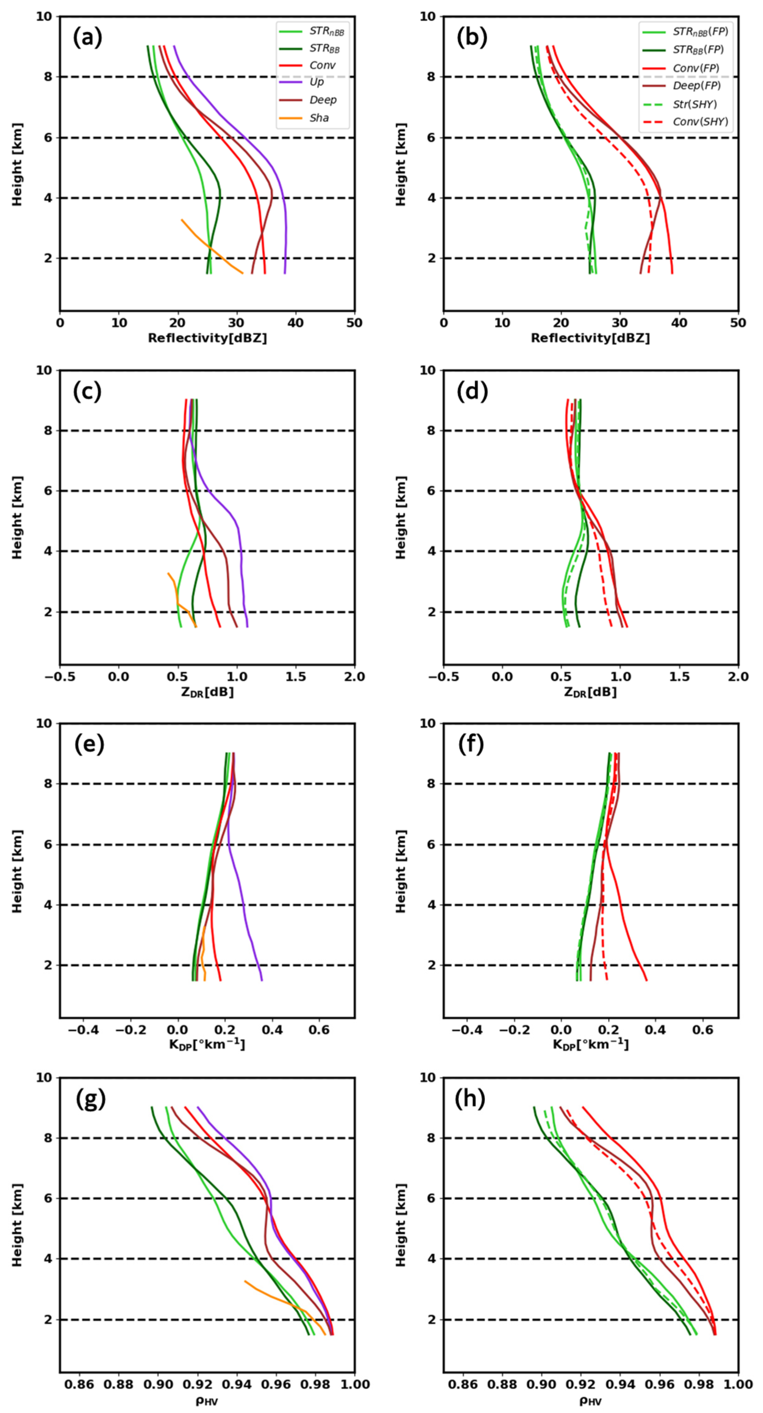
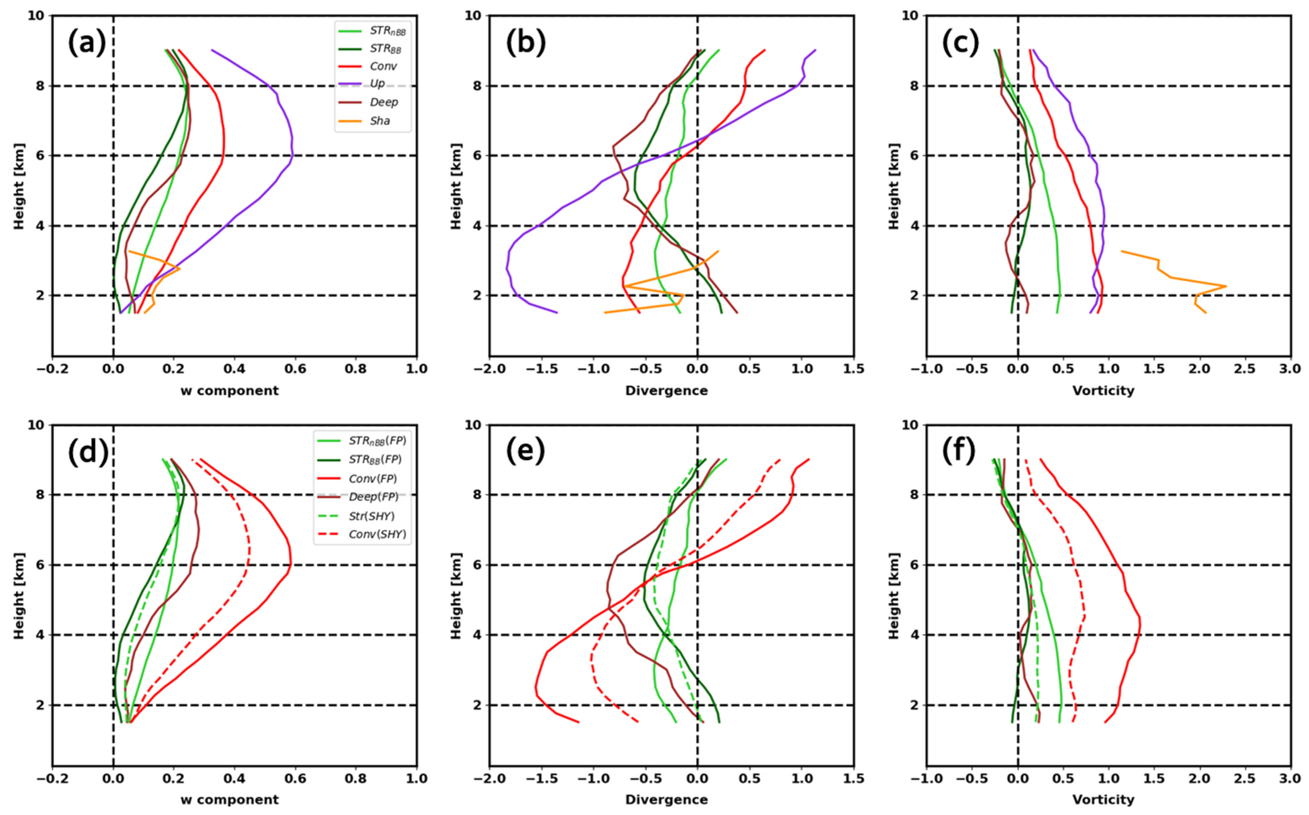
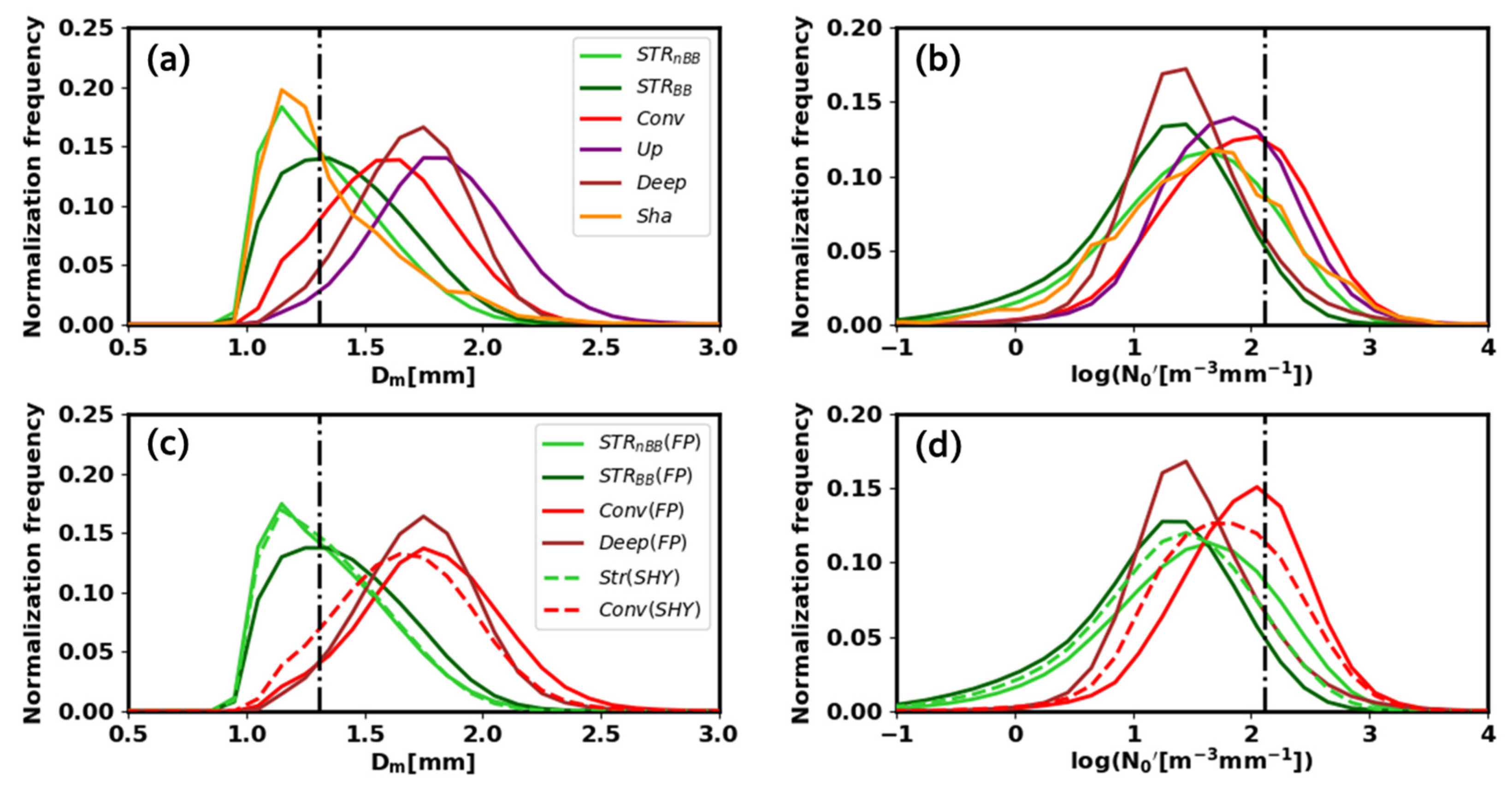
4.2. Physical Properties of Precipitation Types Identified by CP and Traditional Classification Methods

Building upon the classification results and structural comparisons presented in Section 4.1, this subsection further explores the dynamic, microphysical, and radar-observed characteristics of the precipitation types identified by the CP, FP, and SHY algorithms. The analysis utilizes 20 warm-season rainfall cases (Table 1), encompassing a mid-latitude cyclone, Changma front, parallel squall line, and diagonal squall line. The parallel (diagonal) squall line refers to a line-shaped rainfall system that moves parallel (perpendicular) to the orientation of the convective band. These four system types span meso- to synoptic-scale precipitation and collectively represent diverse precipitation growth processes, enabling a comprehensive examination of the classification results.

Figure 7 presents Contoured Frequency by Altitude Diagrams (CFADs) of radar reflectivity for six precipitation types: (a) stratiform with a bright band (STR_BB), (b) stratiform without a bright band (STR_nBB), (c) convection, (d) updraft, (e) deep system, and (f) shallow system. In STR_BB, STR_nBB, and deep systems (Figure 7a,b,e), the reflectivity frequency distributions are predominantly confined below 30 dBZ above 7 km altitude. This pattern resembles the vertical structure of stratiform rain observed by Schumacher and Houze [8], suggesting relatively homogeneous ice-phase growth processes such as diffusional growth occurring under weak vertical motion.

By contrast, convection and updraft regions (Figure 7c,d) exhibit broader reflectivity distributions above the 0 °C level, along with frequent occurrences of higher reflectivity values (>40 dBZ). These features reflect the influence of strong vertical velocities, which promote heterogeneous hydrometeor growth—especially riming and enhanced diffusional growth—as noted in prior studies [8,51]. These mechanisms support the rapid development of precipitation particles within convective updrafts. In the case of shallow systems (Figure 7f), cloud tops remain below 4.5 km, and the reflectivity distribution rapidly shifts toward higher values near the surface. This behavior is indicative of the warm-rain process, in which collision and coalescence dominate, leading to a rapid increase in reflectivity in the lower atmosphere.

Figure 8 presents the mean vertical profiles of dual-polarization radar variables for different precipitation types identified by the CP, FP, and SHY algorithms. In STR_BB and deep systems (Figure 8a), the reflectivity (Z_H) peaks at approximately 4.25 km with values of 27.4 dBZ and 36.2 dBZ, respectively, consistent with the melting layer height during warm-season events over the Korean Peninsula. This peak corresponds to the bright band signature. By contrast, STR_nBB does not exhibit such features as it includes early or decaying stages of stratiform precipitation systems [4]. In these types, Z_H values decrease in the rain region (below 4 km), but microphysical differences emerge: the vertical Z_DR and K_DP profiles for the deep system increase and decrease, respectively. According to the microphysical fingerprints [50] introduced in Section 3.2, breakup or evaporation likely dominate STR_BB near the surface, while size sorting appears to be a major process in the deep system type. The updraft category shows markedly higher Z_H, Z_DR, and K_DP values below 6 km, peaking at 38.3 dBZ, 1.19 dB, and 0.36 °km⁻¹, respectively (Figure 8a,c,e). Between 4 and 6 km—just above the freezing level— Z_DR, and K_DP range from 0.76 to 1.03 dB and 0.22 to 0.28 °km⁻¹, respectively. These values suggest that large raindrops are lifted by strong vertical motion, and the updraft signature is clearly captured by dual-polarization variables, emphasizing their usefulness for updraft detection. For convection and shallow systems, both Z_H and Z_DR increase sharply toward the surface, suggesting dominant growth by warm-rain processes such as collision and coalescence. The K_DP profile shows less distinct trends, but the combined increase in Z_H, Z_DR, and K_DP (Figure 8a–c) supports the likelihood of active coalescence. Notably, Z_DR values in the shallow system remain below 0.6 dB, indicating smaller drop sizes. The ρ_HV profiles (Figure 8g) remain above 0.9 across all types, with localized minima near the melting layer due to the coexistence of water and ice hydrometeors. FP and SHY methods are compared in Figure 8b,d,f,h. In FP, the Z_H, Z_DR, and K_DP profiles for convection and deep systems tend to be higher than those of CP, likely due to overestimation or misclassification of strong updrafts as convective or deep regions. This tendency aligns with cross-sectional patterns in Figure 5e and Figure 6e. The SHY method, by contrast, fails to capture the bright band signature in stratiform precipitation, further underscoring the limitations of its classification approach.

Figure 9 illustrates the dynamic characteristics derived from WISSDOM for various precipitation types. The vertical air motions (w-component; Figure 9a) of deep systems and stratiform regions decrease with height up to approximately 3 km while maintaining positive values. Above the freezing level, the vertical velocity increases with height for all types except shallow systems. The updraft regions show a peak vertical velocity of ~0.6 m s⁻¹ at ~6 km altitude, in contrast to ~2.4 m s⁻¹ observed in tropical deep convection around 9 km by Schumacher et al. [51]. This difference is attributed to climatological differences, as Schumacher et al. focused on tropical monsoon systems over Darwin, Australia, whereas the present study targets mid-latitude rainfall systems over the Korean Peninsula. Moreover, their profiles included extreme updrafts exceeding 15–18 m s⁻¹ above 7 km. The observed peak of w in our updraft category aligns with increased ZDR and KDP values at similar altitudes, supporting the use of dual-polarization variables above the melting layer to infer updrafts. In shallow systems, vertical motion peaks occur at lower altitudes (0–3 km), consistent with warm-rain processes.

Figure 9b shows vertical profiles of divergence. In STR_BB and deep systems, upper-level divergence is observed above ~8.5 km, with low-level divergence below ~3 km, and convergence in the mid-level (~3–8 km). These patterns are associated with upper-level heating and lower-level cooling, consistent with Homeyer et al. [52]. In contrast, convection and updraft regions exhibit strong low-level convergence (below 6.5 km) and pronounced upper-level divergence, indicating intense latent heating above 3 km. The level of non-divergence (LND) for STR_BB, STR_nBB, and deep systems occurs near 8.5 km, whereas for convection and updraft, it appears to be 6.2 km. Shallow systems show a similar structure to convection but with weaker divergence magnitudes.

Relative vorticity profiles (Figure 9c) further distinguish the dynamic structures. Cyclonic vorticities in STR_BB and deep systems are prominent between 4 and 7 km, consistent with Bosart [53]. In convection, cyclonic vorticity extends up to 9 km with a peak near 2 km, in line with results from Hopper and Schumacher [54]. STR_nBB also displays cyclonic vorticity up to ~7 km, albeit weaker. The updraft profile closely follows that of convection, but with a higher vorticity peak around 4.5 km. Interestingly, shallow systems exhibit strong cyclonic vorticity at the lower levels, likely driven by active growth processes associated with upward motion.

The vertical profiles of w, divergence, and vorticity for FP and SHY algorithms are shown in Figure 9d–f. For FP and SHY, the convective and deep system profiles exhibit stronger upward motion and cyclonic vorticity at upper levels compared to CP, likely due to the inclusion of updraft signatures in their broader convective classifications. Meanwhile, the STR_BB and STR_nBB profiles in FP closely match those in CP as both use the same classification parameters based on feature profiles (see Figure 4). These results demonstrate that the CP method allows for more precise separation of dynamic features across precipitation types than SHY or FP, which tend to merge distinct dynamic regimes due to less detailed classification schemes.

Figure 10 presents the probability density functions (PDFs) of the generalized microphysical parameters—mass-weighted mean diameter (D_m) and intercept parameter (N₀′)—for each precipitation type, as derived from the rain region. The dashed-dotted vertical lines indicate the mean values obtained from the 2 DVD dataset over the Korean Peninsula: 1.31 mm for D_m and log(N₀′) = 2.01 (i.e., N₀′≈102.11 m⁻³ mm⁻¹). In panel (a), the PDFs of D_m for convection, updraft, and deep systems are right shifted relative to the mean, reflecting the presence of larger hydrometeors in these categories. Conversely, STR_nBB and shallow systems show distributions left-shifted below the mean D_m, indicating the dominance of smaller raindrops. In panel (b), the log N₀′ distributions for all precipitation types are slightly left shifted from the mean. This pattern may reflect the microphysical structure of the selected rainfall cases, which mostly represent deep convective systems associated with intense precipitation, as previously documented in Bang et al. [20].

For convective regions (convection and updraft), both D_m and N₀′ peak at relatively high values: D_m > 1.5 mm and log(N₀′) > 1.7, which is consistent with findings by Penide et al. [6]. These features correlate well with the large Z_DR and K_DP values observed in the vertical profiles of these types (Figure 8b,c), implying active coalescence. In contrast, the deep system shows a D_m distribution between 1.5 and 2.0 mm, overlapping with those of convective types. However, its log N₀′ distribution (101.1–101.6 m⁻³ mm⁻¹) is more closely aligned with STR_BB, suggesting that deep systems share similarities in number concentration with stratiform clouds but have larger drop sizes. Notably, the shallow system exhibits a relatively right-shifted log N₀′ compared to STR_BB, indicating a higher drop concentration despite its smaller D_m. This may result from enhanced low-level Z_H, Z_DR, and K_DP (below 2 km), supported by weak upward motion (Figure 9a), indicating a dominant warm-rain process.

The PDFs for SHY and FP stratiform categories closely match those of CP, reaffirming classification consistency in stratiform regions (also supported by Penide et al. [6]). However, the FP algorithm’s convective category exhibits a further shift toward larger D_m and higher N₀′ than the CP, suggesting that updraft features may have been overrepresented in its convective classification. These findings underscore the distinct microphysical signatures of each precipitation type. The CP classification method provides enhanced capability to differentiate between rainfall regimes based on D_m and N₀′ distributions, highlighting its utility in microphysical characterization of diverse rain systems.

5. Discussion

The CP algorithm contributes to providing a more detailed classification of precipitation types. We proved that CP is more effective than previous studies, such as SHY and FP, for the classification of detailed precipitation types for mid-latitude cyclone cases during the warm season. From a quantitative perspective, CP achieved a higher probability of detection (POD) and critical success index (CSI) values than SHY and FP for classifying precipitation types (see Table 6). In addition, comparative analysis of vertical cross-sections of Z_H (Figure 5 and Figure 6) confirms the improved ability of CP to delineate detailed vertical structures. These findings indicate that CP is more effective than conventional approaches for precipitation classification in the warm season. However, the quantitative evaluation was conducted using a limited number of rainfall cases (Table 1). Future studies should validate the CP algorithm using long-term observational datasets to improve the generality and robustness of its classification performance. Furthermore, classifying winter precipitation, such as snowfall, remains challenging due to the absence of a melting layer. Thus, a modified version of the CP algorithm tailored for winter conditions needs to be developed.

The CP method was applied using 3D CAPPI datasets from the WRC of KMA. These high-resolution datasets are well suited for the Korean Peninsula but are geographically constrained. Nonetheless, the application of CP demonstrates its utility in improving the understanding of precipitation systems in complex mid-latitude environments. To enhance its universality, validation using radar data from different climatic and geographic regions (e.g., East Asia, the United States, or Europe) is recommended.

The subcategorization scheme within the CP algorithm not only mitigated misclassification of shallow convection and deeply developed stratiform precipitation but also enabled the identification of updraft regions. This has implications for studying the processes of lightning generation. According to Deierling et al. [9], lightning occurrence is closely linked to the fluxes of various ice mass types, such as non-precipitating ice, graupel, and hail. These fluxes can be derived using relationships between radar reflectivity (Z_e) and ice mass content (I), expressed as I = aZ_eᵇ. Building on this, future work will estimate radar-based ice mass fluxes in updraft volumes (defined as contiguous grid regions with vertical velocities above a given threshold) to investigate lightning activity.

The classified precipitation types provided by CP have practical applications in both weather forecasting and hydrological modeling. For example, updraft regions—associated with strong convective motion—can be used in nowcasting to predict severe weather phenomena such as heavy rainfall, hail, and gusty winds. On the other hand, stratiform precipitation, which tends to produce uniform and widespread rainfall, is suitable for modeling surface runoff and area-averaged precipitation in hydrological systems. Additionally, the spatially detailed precipitation fields generated by CP may improve aviation weather forecasts and quantitative precipitation estimation (QPE).

The dynamic and microphysical characteristics of various precipitation types were analyzed using radar and model-based parameters. The results showed that each category exhibits distinct signatures in both dynamic and microphysical variables (Figure 8, Figure 9 and Figure 10). For instance, dual-polarization variables such as Z_H, Z_DR, and K_DP of updraft increased below 6 km altitude, consistent with warm-rain processes involving coalescence. These features were also associated with larger values of D_m and N₀′. In particular, enhanced upper-level divergence in the updraft regions highlights the key role of vertical ascent in organizing convective structures. These results refine the conceptual model of precipitation systems in the East Asian mid-latitude monsoon environment. Nevertheless, further investigation of the thermodynamic vertical structure between stratiform and convective precipitation is crucial for a better understanding of the net heating and cooling processes associated with the growth and decay of hydrometeors. Houze et al. [62] proposed idealized vertical heating profiles for mesoscale convective systems, with convective regions dominated by latent heating from condensation, and stratiform regions showing upper-level heating and lower-level cooling due to melting and evaporation. Lee et al. [63] used brightness temperature (BT) data from GOES-16 and WRF simulations to distinguish between stratiform and convective latent heating profiles. Building on this, we plan to investigate thermodynamic structures of precipitation types using high-resolution BT data from the Geostationary Korea Multi-Purpose Satellite-2A (GK2A), which offers excellent spatiotemporal coverage over the Korean Peninsula.

6. Conclusions

This study proposes a new classification algorithm for precipitation types (CP) that integrates three-dimensional (3D) radar data and temperature fields, addressing the frequent misclassification issues between shallow convection and intense stratiform precipitation in traditional methods. The CP method combines multiple algorithms—Storm Labeling in Three Dimensions (SLTD), the feature parameter-based algorithm (FP), and the advanced subcategorization method (ASM)—to classify precipitation into ten distinct categories, including four non-precipitating and six precipitating types.

The performance of CP was evaluated for mid-latitude precipitation systems during the warm season by comparing it with traditional methods (SHY and FP). Quantitative metrics indicated that CP achieved a higher probability of detection (POD: 0.567–0.571) and critical success index (CSI: 0.068–0.186) than SHY and FP. However, a relatively high false alarm ratio (FAR: 0.784–0.928) was also observed, likely due to threshold settings, limited sample size, and residual noise in the wind data used for ground-truth definition. Qualitative analyses revealed that CP effectively distinguishes between different precipitation types in terms of vertical structure and microphysical characteristics. The radar-derived observation and microphysical variables, including reflectivity (Z_H), specific differential phase (K_DP), differential reflectivity (Z_DR), mass-weighted mean diameter (D_m), and normalized intercept parameter (N₀′), exhibited distinct patterns across stratiform and convective types. Updraft regions classified by CP showed higher K_DP and Z_DR values above the melting layer, indicating active microphysical growth involving graupel and large raindrops. Furthermore, CP captured the dynamical characteristics of each type, such as convergence/divergence patterns and vertical vorticity, which were consistent with the expected physical processes of stratiform, convection, and shallow systems.

The classification capability of CP has potential applications in nowcasting, hydrological modeling, and quantitative precipitation estimation. However, the method was developed using 3D CAPPI datasets over the Korean Peninsula and, thus, may have limited regional applicability. To enhance its universality, further validation is needed using radar observations from different climatic and geographic regions (e.g., other East Asian countries, the United States, or Europe). Future research will focus on refining classification thresholds, incorporating thermodynamic variables and lightning activity to improve classification performance and generalization.

References

1. Starzec, M.; Homeyer, C.R.; Mullendore, G.L. Storm labeling in three dimensions (SL3D): A volumetric radar echo and dual-polarization updraft classification algorithm. Mon. Weather. Rev. 2017, 145, 1127–1145. [Google Scholar] [CrossRef]
2. Lee, T.Y.; Kim, Y. Heavy Precipitation systems over the Korean peninsula and their classification. J. Korean Meteorol. Soc. 2007, 43, 367–396. [Google Scholar]
3. Fabry, F.; Zawadzki, I. Long-termradaroperationsofthemeltinglayerofprecipitationandtheirinterpretation. J. Atmos. Sci. 1995, 52, 838–851. [Google Scholar] [CrossRef]
4. Steiner, M.; Houze, R.A., Jr.; Yuter, S.E. Climatological characterization of three-dimensional storm structure from operational radar and rain gauge data. J. Appl. Meteorol. 1995, 34, 1978–2007. [Google Scholar] [CrossRef]
5. Biggerstaff, M.I.; Listemaa, S.A. An improved scheme for convective/stratiform echo classification using radar reflectivity. J. Appl. Meteorol. 2000, 39, 2129–2150. [Google Scholar] [CrossRef]
6. Penide, G.; Protat, A.; Kumar, V.V.; May, P.T. Comparison of two convective/stratiform precipitation classification techniques: Radar reflectivity texture versus drop size distribution–based approach. J. Atmos. Ocean. Technol. 2013, 30, 2788–2797. [Google Scholar] [CrossRef]
7. Powell, S.W.; Houze, R.A., Jr.; Brodzik, S.R. Rainfall type categorization of radar echoes using polar coordinate reflectivity data. J. Atmos. Ocean. Technol. 2016, 33, 523–538. [Google Scholar] [CrossRef]
8. Schumacher, C.; Houze, R.A., Jr. Stratiform precipitation production over sub-Saharan Africa and the tropical East Atlantic as observed by TRMM. Quart. J. Roy. Meteor. Soc. 2006, 132, 2235–2255. [Google Scholar] [CrossRef]
9. Deierling, W.; Petersen, W.A.; Latham, J.; Ellis, S.; Christian, H.J. The relationship between lightning activity and ice fluxes in thunderstorms. J. Geophys. Res. 2008, 113, D15210. [Google Scholar] [CrossRef]
10. Bringi, V.N.; Chandrasekar, V.; Hubbert, J.; Gorgucci, E.; Randeu, W.L.; Schoenhuber, M. Raindrop size distribution in different climatic regimes from disdrometer and dual-polarized radar analysis. J. Atmos. Sci. 2003, 60, 354–365. [Google Scholar] [CrossRef]
11. Kirsch, B.; Clemens, M.; Ament, F. Stratiform and convective radar reflectivity–rain rate relationships and their potential to improve radar rainfall estimates. J. Appl. Meteorol. Climatol. 2019, 58, 2259–2271. [Google Scholar] [CrossRef]
12. Loh, J.L.; Lee, D.I.; Kang, M.Y.; You, C.H. Classification of rainfall types using parsivel disdrometer and S-band polarimetric radar in central Korea. Remote Sens. 2020, 12, 642. [Google Scholar] [CrossRef]
13. Feng, Z.; Dong, X.Q.; Xi, B.K.; Schumacher, C.; Minnis, P.; Khaiyer, M. Top-of-atmosphere radiation budget of convective core/stratiform rain and anvil clouds from deep convective systems. J. Geophys. Res. 2011, 116, D23202. [Google Scholar] [CrossRef]
14. Dixon, M.; Romatschke, U. Three-dimensional convective–stratiform echo-type classification and convectivity retrieval from radar reflectivity. J. Atmos. Ocean. Technol. 2022, 39, 1685–1704. [Google Scholar] [CrossRef]
15. Lee, J.E.; Jung, S.H.; Kwon, S. Characteristics of the bright band based on quasi-vertical profiles of polarimetric observations from an S-band weather radar Network. Remote Sens. 2020, 12, 4061. [Google Scholar] [CrossRef]
16. Liou, Y.-C.; Chang, Y.-J. A variational multiple–Doppler radar three-dimensional wind synthesis method and its impacts on thermodynamic retrieval. Mon. Wea. Rev. 2009, 137, 3992–4010. [Google Scholar] [CrossRef]
17. Tsai, C.L.; Kim, K.; Liou, Y.C.; Lee, G.; Yu, C.K. Impacts of Topography on Airflow and Precipitation in the Pyeongchang Area Seen from Multiple-Doppler Radar Observations. Mon. Wea. Rev. 2018, 146, 3401–3424. [Google Scholar] [CrossRef]
18. Jorgensen, D.P.; LeMone, M.A. Vertical velocity characteristics of oceanic convection. J. Atmos. Sci. 1989, 46, 621–640. [Google Scholar] [CrossRef]
19. WMO. Guidelines on Surface Station Data Quality Control and Quality Assurance for Climate Applications (WMO-No.1269). 2021. Available online: https://library.wmo.int/idurl/4/57727 (accessed on 17 July 2025).
20. Bang, W.; Lee, G.; Ryzhkov, A.; Schuur, T.; Lim, K.-S.S. Comparison of Microphysical Characteristics between the Southern Korean Peninsula and Oklahoma Using Two-Dimensional Video Disdrometer Data. J. Hydrometeorol. 2020, 21, 2675–2690. [Google Scholar] [CrossRef]
21. Kruger, A.; Krajewski, W.F. Two-dimensional video disdrometer: A description. J. Atmos. Ocean. Technol. 2002, 19, 602–617. [Google Scholar] [CrossRef]
22. Atlas, D.; Srivastava, R.C.; Sckhon, R.S. Doppler radar characteristics of precipitation at vertical incidence. Rev. Geophys. Sp. Phys. 1973, 11, 1–35. [Google Scholar] [CrossRef]
23. Marshall, J.S.; Palmer, W.M.K. The distribution of raindrops with size. J. Meteorol. 1948, 5, 165–166. [Google Scholar] [CrossRef]
24. Ulbrich, C.W. Natural variations in the analytical form of the raindrop size distribution. J. Clim. Appl. Meteorol. 1983, 22, 1764–1775. [Google Scholar] [CrossRef]
25. Auf der Maur, A.N. Statistical tools for drop size distribution: Moments and generalized gamma. J. Atmos. Sci. 2001, 58, 407–418. [Google Scholar] [CrossRef]
26. Carletta, N.D.; Mullendore, G.L.; Starzec, M.; Xi, B.; Feng, Z.; Dong, X. Determining the best method for estimating the observed level of maximum detrainment based on radar reflectivity. Mon. Wea. Rev. 2016, 144, 2915–2926. [Google Scholar] [CrossRef]
27. Short, E.; Lane, T.P.; Vincent, C.L. Objectively diagnosing characteristics of mesoscale organization from radar reflectivity and ambient winds. Mon. Wea. Rev. 2023, 151, 643–662. [Google Scholar] [CrossRef]
28. DeMott, C.A.; Rutledge, S.A. The vertical structure of Toga Coare convection. Part I: Radar echo distributions. J. Atmos. Sci. 1998, 55, 2730–2747. [Google Scholar] [CrossRef]
29. Zipser, E.J. Deep cumulonimbus cloud systems in the tropics with and without lightning. Mon. Wea. Rev. 1994, 122, 1837–1851. [Google Scholar] [CrossRef]
30. Petersen, W.A.; Rutledge, S.A.; Orville, R.E. Cloud-to-ground lightning observations to Toga Coare, selected results and lightning location algorithm. Mon. Wea. Rev. 1996, 124, 602–620. [Google Scholar] [CrossRef]
31. Straka, J.M.; Zrnić, D.S.; Ryzhkov, A.V. Bulk hydrometeor classification and quantification using polarimetric radar data: Synthesis of relations. J. Appl. Meteorol. 2000, 39, 1341–1372. [Google Scholar] [CrossRef]
32. Snyder, J.C.; Ryzhkov, A.V.; Kumjian, M.R.; Khain, A.P.; Picca, J. A ZDR Column Detection Algorithm to Examine Convective Storm Updrafts. Weather Forecast. 2015, 30, 1819–1844. [Google Scholar] [CrossRef]
33. Loney, M.L.; Zrnić, D.S.; Straka, J.M.; Ryzhkov, A.V. Enhanced Polarimetric Radar Signatures above the Melting Level in a Supercell Storm. J. Appl. Meteorol. 2002, 41, 1179–1194. [Google Scholar] [CrossRef]
34. Van Lier-Walqui, M.; Fridlind, A.M.; Ackerman, A.S.; Collis, S.; Helmus, J.; MacGorman, D.R.; North, K.; Kollias, P.; Posselt, D.J. On Polarimetric Radar Signatures of Deep Convection for Model Evaluation: Columns of Specific Differential Phase Observed during MC3E. Mon. Wea. Rev. 2016, 144, 737–758. [Google Scholar] [CrossRef] [PubMed]
35. Musil, D.J.; Heymsfield, A.J.; Smith, P.L. Microphysical characteristics of a well-developed weak echo region in a high plains su-percell thunderstorm. J. Appl. Meteorol. Climatol. 1986, 25, 1037–1051. [Google Scholar] [CrossRef]
36. Calhoun, K.M.; MacGorman, D.R.; Ziegler, C.L.; Biggerstaff, M.I. Evolution of Lightning Activity and Storm Charge Relative to Dual-Doppler Analysis of a High-Precipitation Supercell Storm. Mon. Wea. Rev. 2013, 141, 2199–2223. [Google Scholar] [CrossRef]
37. Awaka, J.; Iguchi, T.; Okamoto, K. TRMM PR Standard Algorithm and its Performance on Bright Band Detection. J. Meteorol. Soc. Jpn. 2009, 87, 31–52. [Google Scholar] [CrossRef]
38. Kumjian, M.R.; Ryzhkov, A.V.; Trömel, S.; Diederich, M.; Mühlbauer, K.; Simmer, C. Retrievals of Warm-Rain Microphysics Using X-Band Polarimetric Radar Data. Extended Abstracts. In Proceedings of the 92nd Annual Meeting of the American Meteorological Society, New Orleans, LA, USA, 26 January 2012; p. 406. [Google Scholar]
39. Tabary, P.; Henaff, A.; Vulpiani, G.; Parent-du-Chatelet, J.; Gourley, J.J. Melting Layer Characterization and Identification with a C-Band Dual-Polarization Radar: A Long-Term Analysis. In Proceedings of the Fourth European Conference on Radar in Meteorology and Hydrology (ERAD 2006), Barcelona, Spain, 18–22 September 2006; Servei Meteorològic de Catalunya: Barcelona, Spain, 2006; pp. 17–20. [Google Scholar]
40. Shusse, Y.; Takahashi, N.; Nakagawa, K.; Satoh, S.; Iguchi, T. Polarimetric radar observation of the melting layer in a convective rainfall system during the rainy season over the East China sea. J. Appl. Meteorol. Climatol. 2011, 50, 354–367. [Google Scholar] [CrossRef]
41. Williams, C.R.; Ecklund, W.L.; Gage, K.S. Classification of Precipitating Clouds in the Tropics Using 915-MHz Wind Profilers. J. Atmos. Ocean. Technol. 1995, 12, 996–1012. [Google Scholar] [CrossRef]
42. Boudevillain, B.; Andrieu, H. Assessment of vertically integrated liquid (VIL) water content radar measurement. J. Atmos. Ocean. Technol. 2003, 20, 807–819. [Google Scholar] [CrossRef]
43. Iguchi, T.; Seto, S.; Meneghini, R.; Yoshida, N.; Awaka, J.; Le, M.; Chandrasekar, V.; Brodzik, S.; Tanelli, S.; Kanemaru, K.; et al. GPM/DPR Level-2 Algorithm Theoretical Basis Document; NASA Technical Report. 2024. Available online: https://gpm.nasa.gov/resources/documents/gpm-dpr-level-2-algorithm-theoretical-basis-document-atbd (accessed on 17 July 2025).
44. Houze, R.A. Observed structure of mesoscale convective systems and implications for large-scale heating. Q. J. R. Meteorol. Soc. 1989, 115, 425–461. [Google Scholar] [CrossRef]
45. Deng, M.; Kollias, P.; Feng, Z.; Zhang, C.; Long, C.N.; Kalesse, H.; Chandra, A.; Kumar, V.V.; Protat, A. Stratiform and convective precipitation observed by multiple radars during the DYNAMO/AMIE experiment. J. Appl. Meteorol. Climatol. 2014, 53, 2503–2523. [Google Scholar] [CrossRef]
46. Carr, N.; Kirstetter, P.E.; Gourley, J.J.; Hong, Y. Polarimetric Signatures of Midlatitude Warm-Rain Precipitation Events. J. Appl. Meteor. Climatol. 2017, 56, 697–711. [Google Scholar] [CrossRef]
47. Handler, S.L.; Homeyer, C.R. Radar-observed bulk microphysics of midlatitude leading line trailing stratiform mesoscale convective systems. J. Appl. Meteor. Climatol. 2018, 57, 2231–2248. [Google Scholar] [CrossRef]
48. Huang, H.; Chen, F. Precipitation Microphysics of Tropical Cyclones Over the Western North Pacific Based on GPM DPR Observations: A Preliminary Analysis. J. Geophys. Res. Atmos. 2019, 124, 3124–3142. [Google Scholar] [CrossRef]
49. Rinehart, R.E. Radar for Meteorologists, 4th ed.; Rinehart Publications: Columbia, MO, USA, 2004; 482p, ISBN 0-9658002-1-0. [Google Scholar]
50. Kumjian, M.R.; Prat, O.P.; Reimel, K.J.; van Lier-Walqui, M.; Morrison, H.C. Dual-Polarization Radar Fingerprints of Precipitation Physics: A Review. Remote Sens. 2022, 14, 3706. [Google Scholar] [CrossRef]
51. Schumacher, C.; Stevenson, S.N.; Williams, C.R. Vertical Motions of the Tropical Convective Cloud Spectrum over Darwin, Australia: Vertical Motions of the Tropical Convective Cloud Spectrum. Q. J. R. Meteorol. Soc. 2015, 141, 2277–2288. [Google Scholar] [CrossRef]
52. Homeyer, C.; Schumacher, C.; Hopper, L.J., Jr. Assessing the applicability of the tropical convective-stratiform paradigm in the extratropics using radar divergence profiles. J. Clim. 2014, 27, 6673–6686. [Google Scholar] [CrossRef]
53. Bosart, L.F. Kinematic vertical motion and relative vorticity profiles in a long-lived midlatitude convective system. J. Atmos. Sci. 1986, 43, 1297–1300. [Google Scholar] [CrossRef]
54. Hopper, L.J., Jr.; Schumacher, C. Modeled and observed variations in storm divergence and stratiform rain production in southeastern Texas. J. Atmos. Sci. 2012, 69, 1159–1181. [Google Scholar] [CrossRef]
55. Lee, G.; Zawadzki, I.; Szyrmer, W.; Sempere-Torres, D.; Uijlenhoet, R. A General Approach to Double-Moment Normalization of Drop Size Distributions. J. Appl. Meteorol. 2004, 43, 264–281. [Google Scholar] [CrossRef]
56. Lee, G.; Bringi, V.; Thurai, M. The retrieval of drop size distribution parameters using a Dual-polarimetric radar. Remote Sens. 2023, 15, 1063. [Google Scholar] [CrossRef]
57. Mishchenko, M.I.; Travis, L.D.; Mackowski, D.W. T-matrix computations of light scattering by nonspherical particles: A review. J. Quant. Spectrosc. Radiat. Transf. 1996, 55, 535–575. [Google Scholar] [CrossRef]
58. Thurai, M.; Huang, G.J.; Bringi, V.N.; Randeu, W.L.; Schönhuber, M. Drop shapes, model comparisons, and calculations of polarimetric radar parameters in rain. J. Atmos. Ocean. Technol. 2007, 24, 1019–1032. [Google Scholar] [CrossRef]
59. Brandes, E.A.; Zhang, G.; Vivekanandan, J. Drop size distribution retrieval with polarimetric radar: Model and application. J. Appl. Meteorol. 2004, 43, 461–475. [Google Scholar] [CrossRef]
60. Cao, Q.; Zhang, G.; Brandes, E. Analysis of video disdrometer and polarimetric radar data to characterize rain microphysics in Oklahoma. J. Appl. Meteorol. Climatol. 2008, 47, 2238–2255. [Google Scholar] [CrossRef]
61. Kwon, S.; Jung, S.-H.; Lee, G. A case study on microphysical characteristics of mesoscale convective system using generalized DSD parameters retrieved from dual-polarimetric radar observations. Remote Sens. 2020, 12, 1812. [Google Scholar] [CrossRef]
62. Houze, R.A., Jr. Mesoscale convective systems. Rev. Geophys. 2004, 42, RG4003. [Google Scholar] [CrossRef]
63. Lee, Y.; Kummerow, C.D.; Zupanski, M. Latent heating profiles from GOES-16 and its impacts on precipitation forecasts. Atmos. Meas. Tech. 2022, 15, 7119–7136. [Google Scholar] [CrossRef]
Figure 1. The lowest observable height (color) map of the KMA dual-polarization radar network, with the dashed rectangular region representing the WISSDOM field.
Remotesensing 17 02506 g001
Figure 2. A flowchart of the quality control procedure for 3D wind components. The arrows indicate the sequential steps in the QC process. The variable x is a proxy for the wind components (u, v, w) and their respective thresholds. The parameter σ denotes the local standard deviation within a 5 × 5 grid window used for the horizontal variation test. The indices i, j, k represent the longitude, latitude, and vertical levels, respectively.
Remotesensing 17 02506 g002
Figure 3. A comparison of Contoured Frequency by Altitude Diagrams (CFADs) of vertical wind components (w) in the updraft region before (a) and after (b) quality control.
Remotesensing 17 02506 g003
Figure 4. A flowchart of the overall CP method. The blue, yellow, and green rounded rectangles represent the classification criteria used in SLTD, FP, and ASM, respectively. ETH refers to the echo top height of ZH, and h0 denotes the height of the 0 °C isotherm (melting layer). CMAXZ represents the column-maximum ZH in each grid column, while Zpeak indicates the local maximum ZH within the −5 to 5 °C layer. UVIL and UMZ correspond to the VIL and the MZ in the upper layer, respectively. The BL_ratio is defined as the ratio of the MZ in the bright band (BMZ) region to that in the lower layer (LMZ). STRnBB and STRBB refer to stratiform precipitation without and with a bright band, respectively.
Remotesensing 17 02506 g004
Figure 5. Precipitation classification and reflectivity features of a heavy rainfall event associated with the Changma front observed at 08:00 UTC on 29 June 2019. (Top) Precipitation types identified by (a) CP, (b) FP, and (c) SHY algorithms. (Bottom) (d) 3D CAPPI reflectivity at 3 km altitude and (e) vertical cross-section of reflectivity (ZH) along the A–B line shown in panels (ad).
Remotesensing 17 02506 g005
Figure 6. Same as Figure 5, but for a squall line associated with a cold front observed at 08:00 UTC on 18 May 2020. (Top) Precipitation types identified by (a) CP, (b) FP, and (c) SHY algorithms. (Bottom) (d) 3D CAPPI reflectivity at 3 km altitude and (e) vertical cross-section of reflectivity (ZH) along the A–B line shown in panels (ad).
Remotesensing 17 02506 g006
Figure 7. The CFADs of radar variables for (a) StrnBB, (b) StrBB, (c) convection, (d) updraft, (e) deep system, and (f) shallow system, using rain cases during warm seasons. The colors indicate the log-normalized frequencies.
Remotesensing 17 02506 g007
Figure 8. Mean vertical profiles of dual-polarization radar variables for different precipitation types. Panels (ad) on the left show profiles of ZH, ZDR, KDP, and ρHV, respectively, for the CP classification. Panels (eh) on the right show the corresponding profiles for the FP (solid lines) and SHY (dashed lines) classifications. The color lines represent precipitation types: stratiform without a bright band (lime green), stratiform with a bright band (dark green), convection (red), updarft (purple), deep systems (brown), and shallow systems (orange).
Remotesensing 17 02506 g008
Figure 9. Mean vertical profiles of dynamical variables derived from WISSDOM for different precipitation types. Panels (ac) show profiles of the vertical wind component (w), divergence, and vorticity, respectively, for the CP classification. Panels (df) display the corresponding profiles for the FP (solid lines) and SHY (dashed lines) classifications. The color lines indicate the precipitation types, which follow the same color scheme as in Figure 8.
Remotesensing 17 02506 g009
Figure 10. Probability density functions (PDFs) of microphysical variables for different precipitation types. Panels (a,b) show the PDFs of mass-weighted mean diameter (Dm) and normalized intercept parameter (logN0′), respectively, for the CP classification. Panels (c,d) present the corresponding distributions for the FP (solid lines) and SHY (dashed lines) classifications. The color lines indicate the precipitation types, following the same color scheme as in Figure 8. Dashed black lines represent the mean values derived from the 2 DVD dataset.
Remotesensing 17 02506 g010