
An Interpretable Machine Learning Framework for Unraveling the Dynamics of Surface Soil Moisture Drivers

 ,
,  , , ,
, , , 
Abstract

1. Introduction
2. Materials and Methods
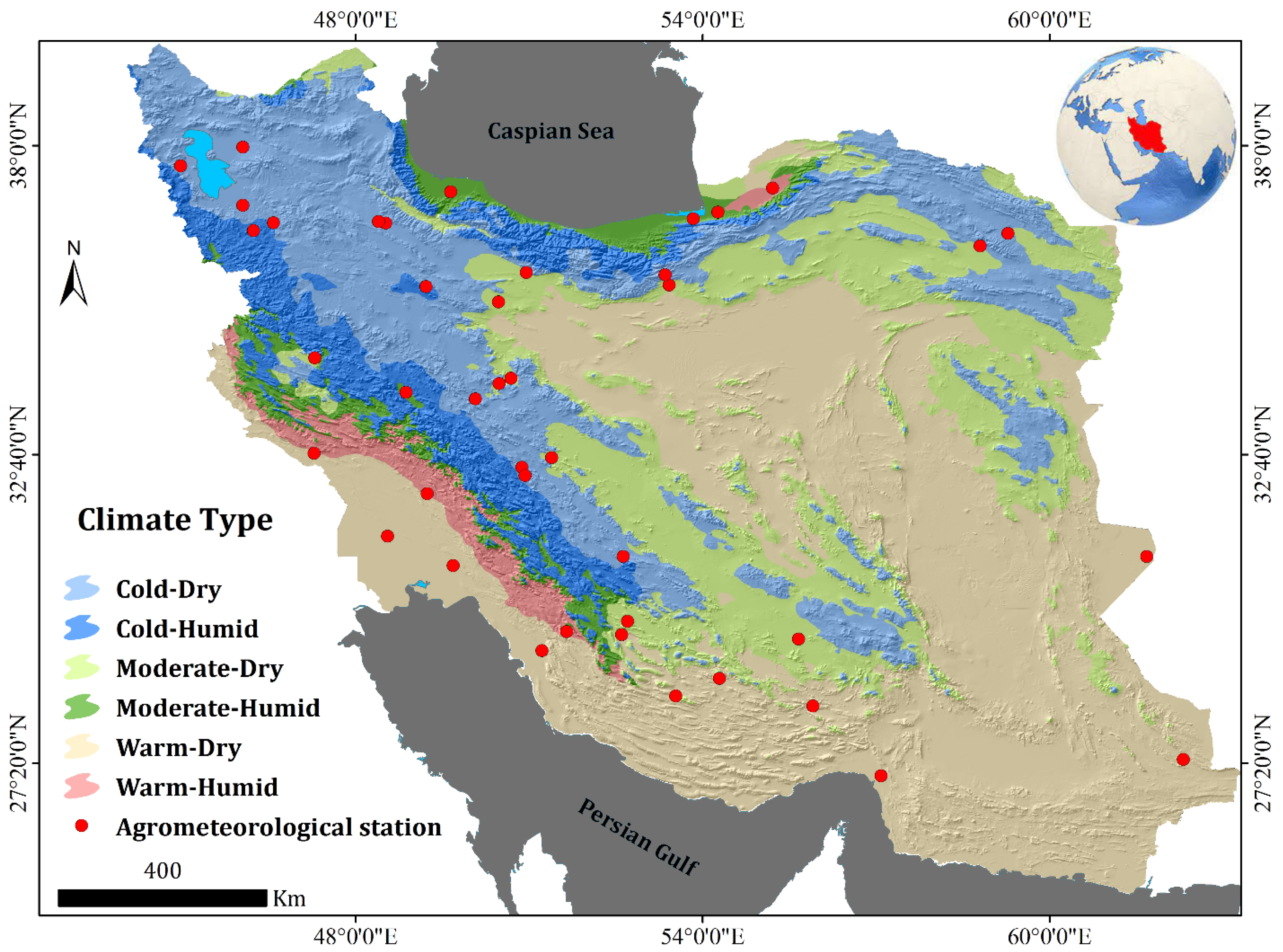
2.1. Study Area
2.2. Datasets
2.2.1. SSM Data

| Data Name | Institution | Examined Period | Spatial Resolution | Temporal Resolution | Reference |
|---|---|---|---|---|---|
| In situ | IMO | 2015–2023 | point location | daily | [39] |
| SMAP Level 4 | NASA | 2015–2023 | 9 km × 9 km | daily | [52] |
| MERRA-2 | NASA | 2015–2023 | 56 km × 70 km | daily | [53] |
| CFSv2 | NCEP | 2015–2023 | 22 km × 22 km | daily | [54] |
2.2.2. Factors Influencing SSM
| Type | Dataset | Source | Spatial Resolution | Reference |
|---|---|---|---|---|
| Dynamic | Precipitation | In situ observations | point location | [39] |
| Potential evapotranspiration | MODIS | 500 m | [61] | |
| Solar radiation | ERA5-Land | 11 km | [62] | |
| Wind speed | ERA5-Land | 11 km | [62] | |
| Normalized difference vegetation index | Sentinel-2 | 10 m | [64] | |
| Groundwater table depth | In situ observations | point location | [44] | |
| Static | Distance from water bodies | NOAA | - | [65] |
| Clay fraction | SoilGrids | 250 m | [66] | |
| Organic matter fraction | SoilGrids | 250 m | [66] | |
| Elevation | ALOS AW3D30 | 30 m | [67] | |
| Topography roughness index | ALOS AW3D30 | 30 m | [67] |
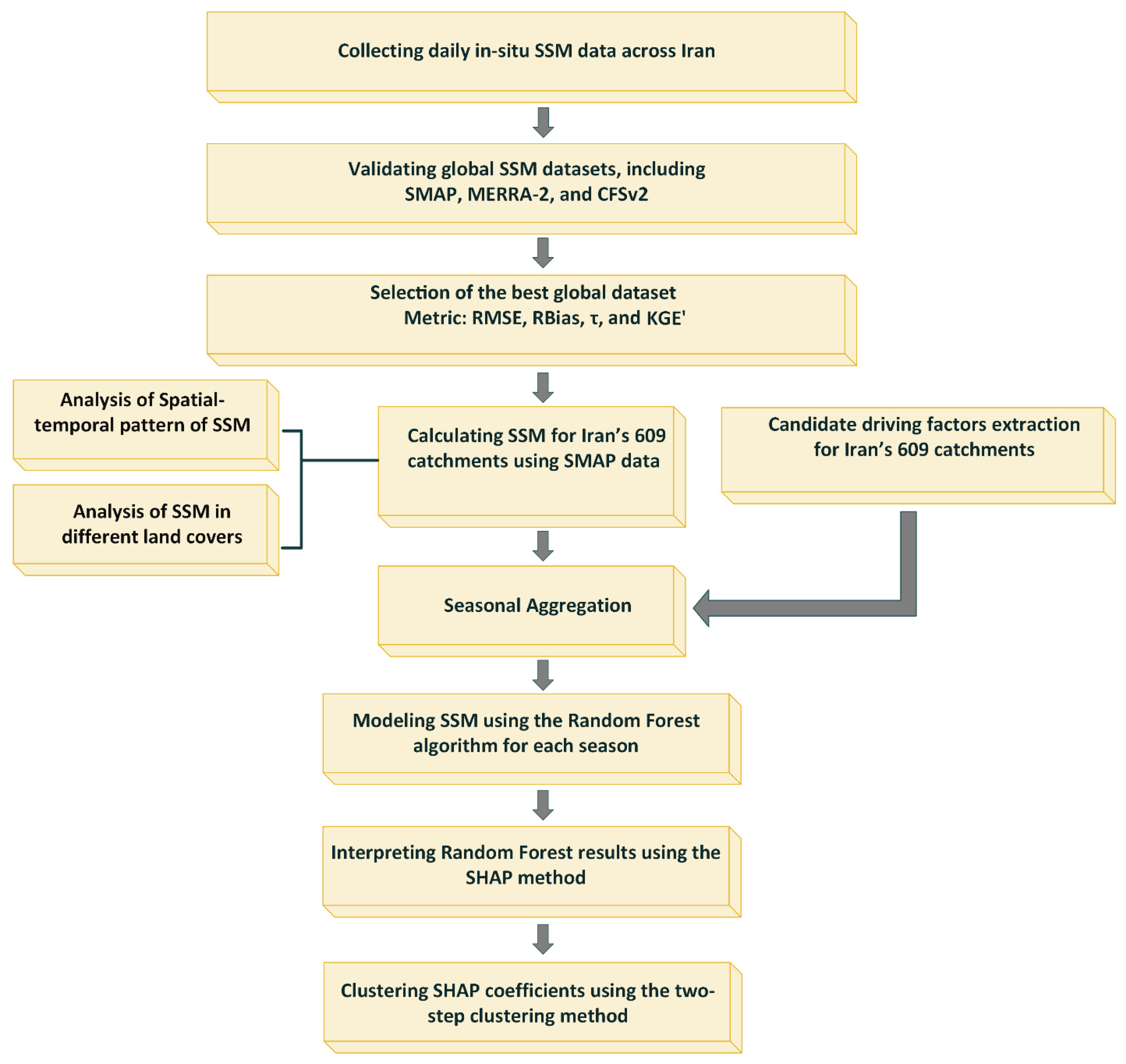
2.3. Methods
2.3.1. Statistical Metrics
2.3.2. Random Forest (RF)
2.3.3. SHAP
2.3.4. Cluster Analysis
3. Results and Discussion
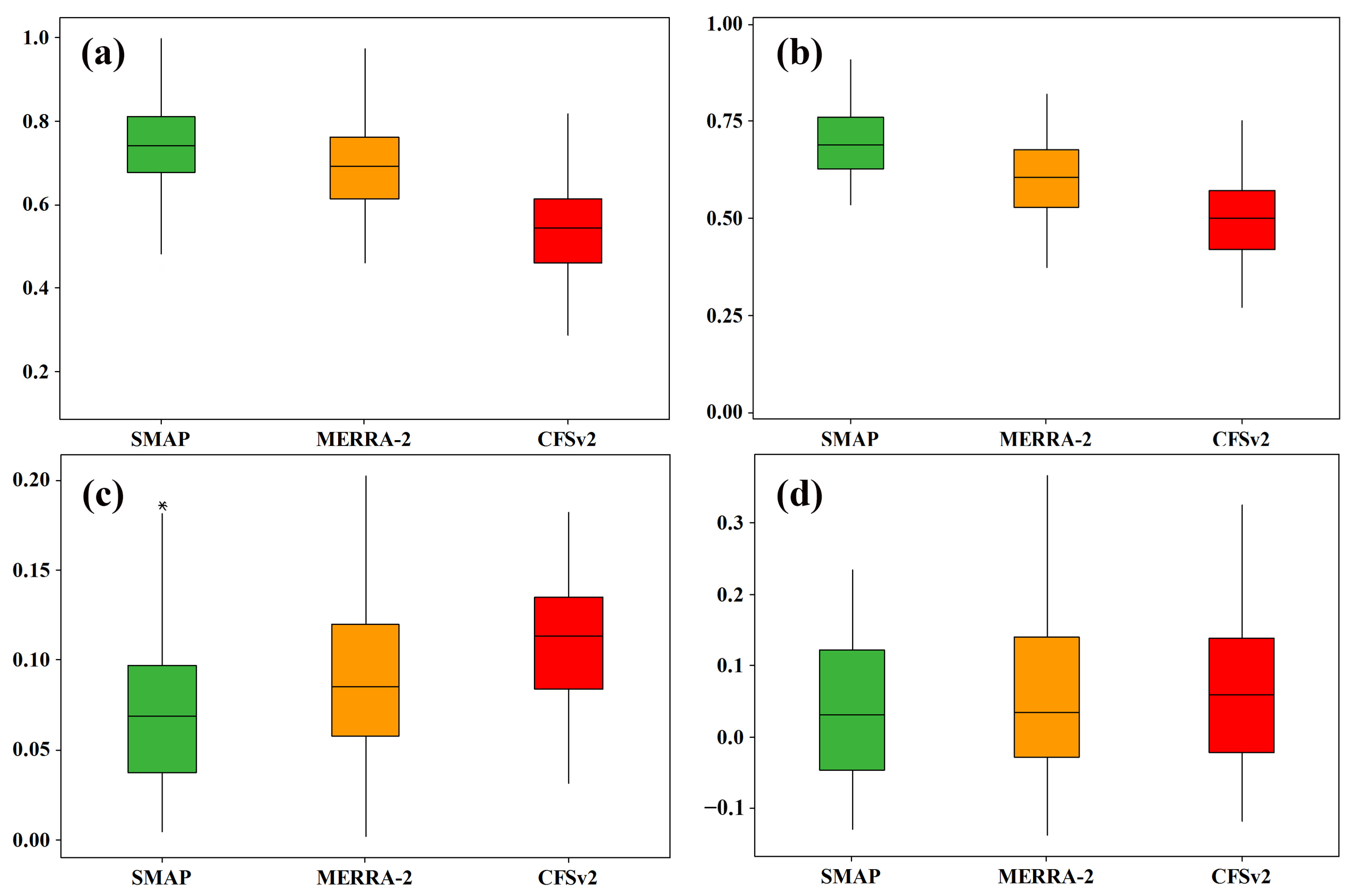
3.1. Performances of SSM Products
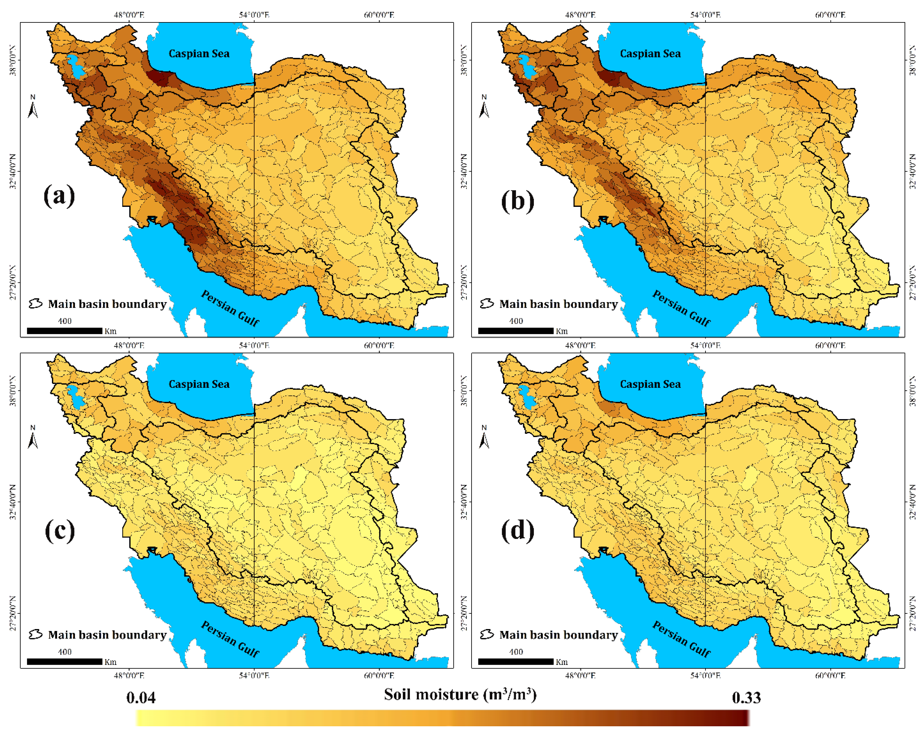
3.2. Spatial-Temporal Pattern of SSM
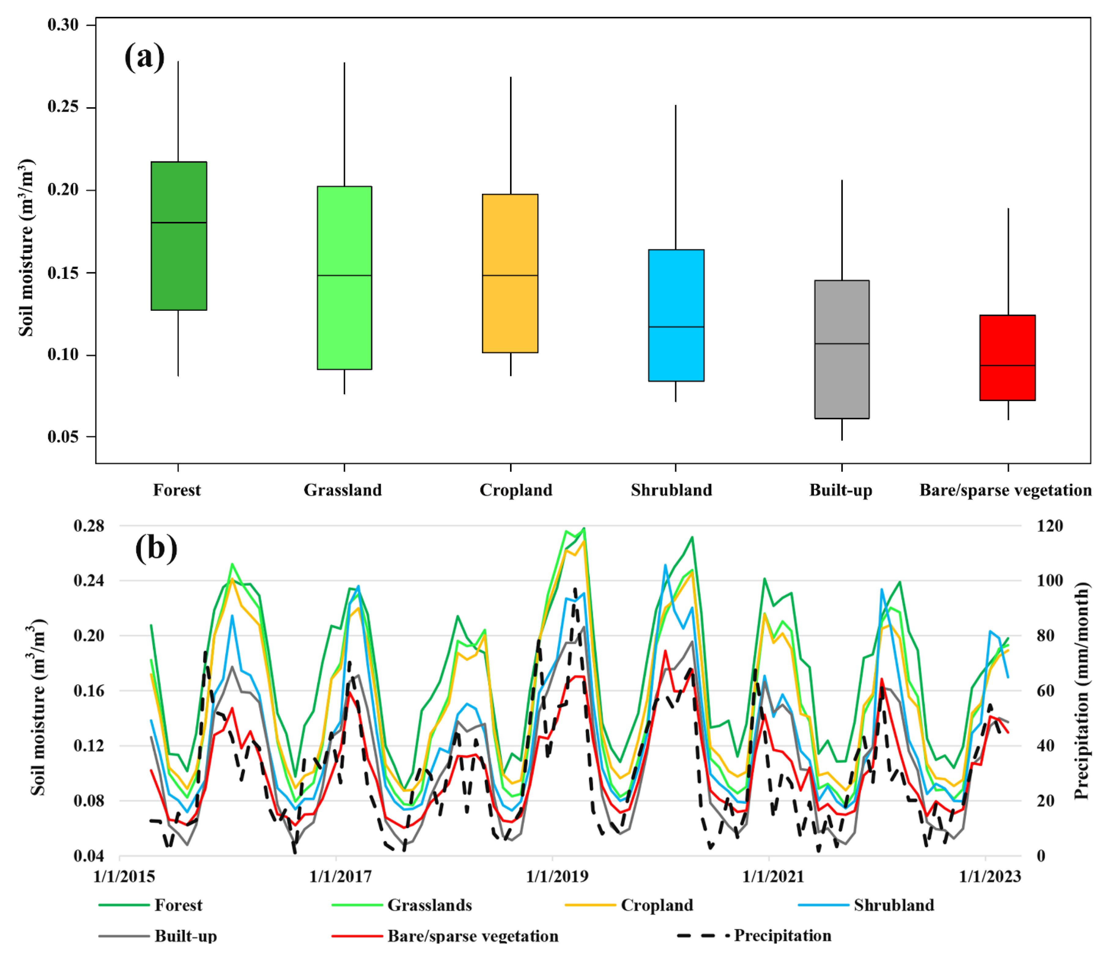
3.3. SSM in Different Land Covers
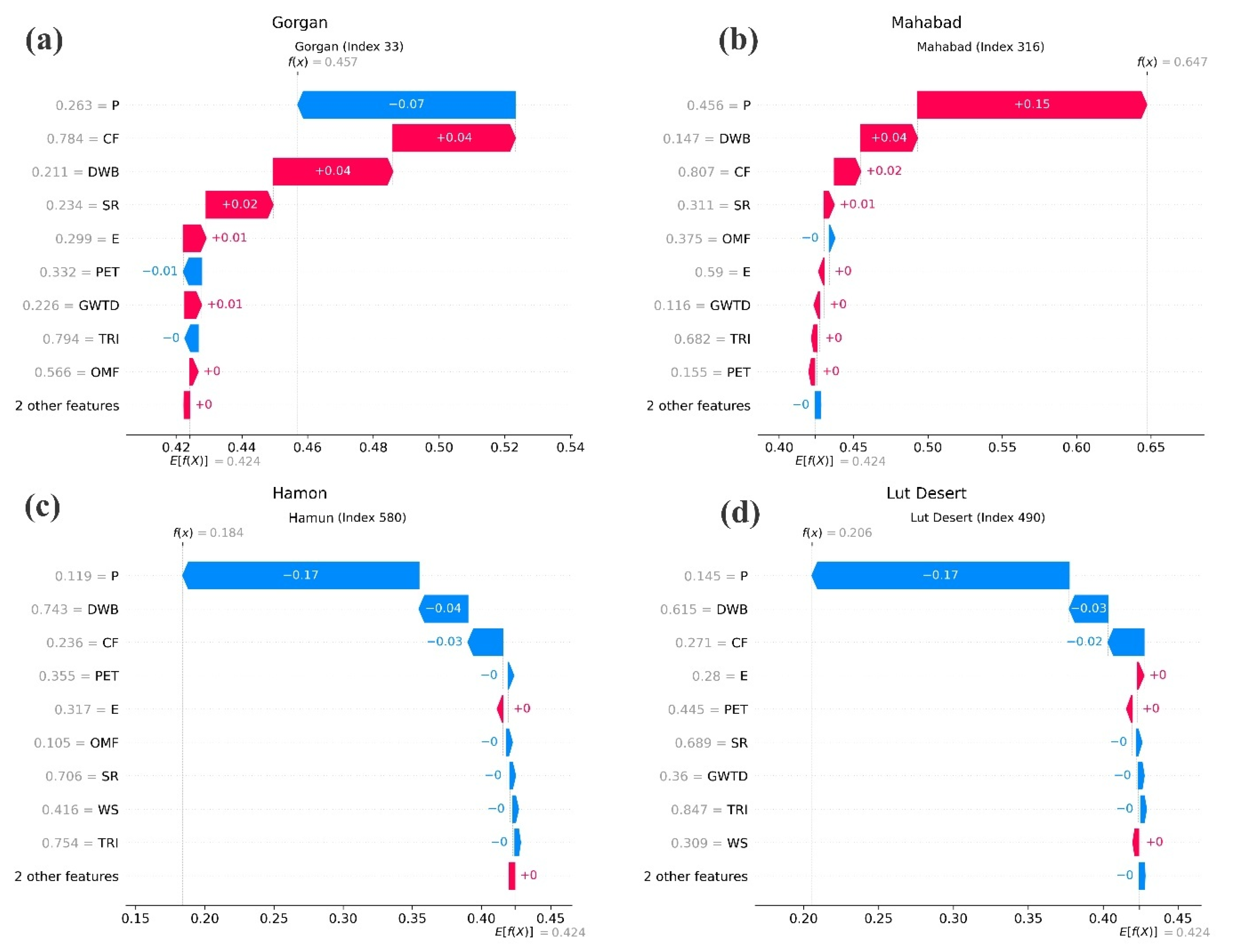
3.4. RF and SHAP
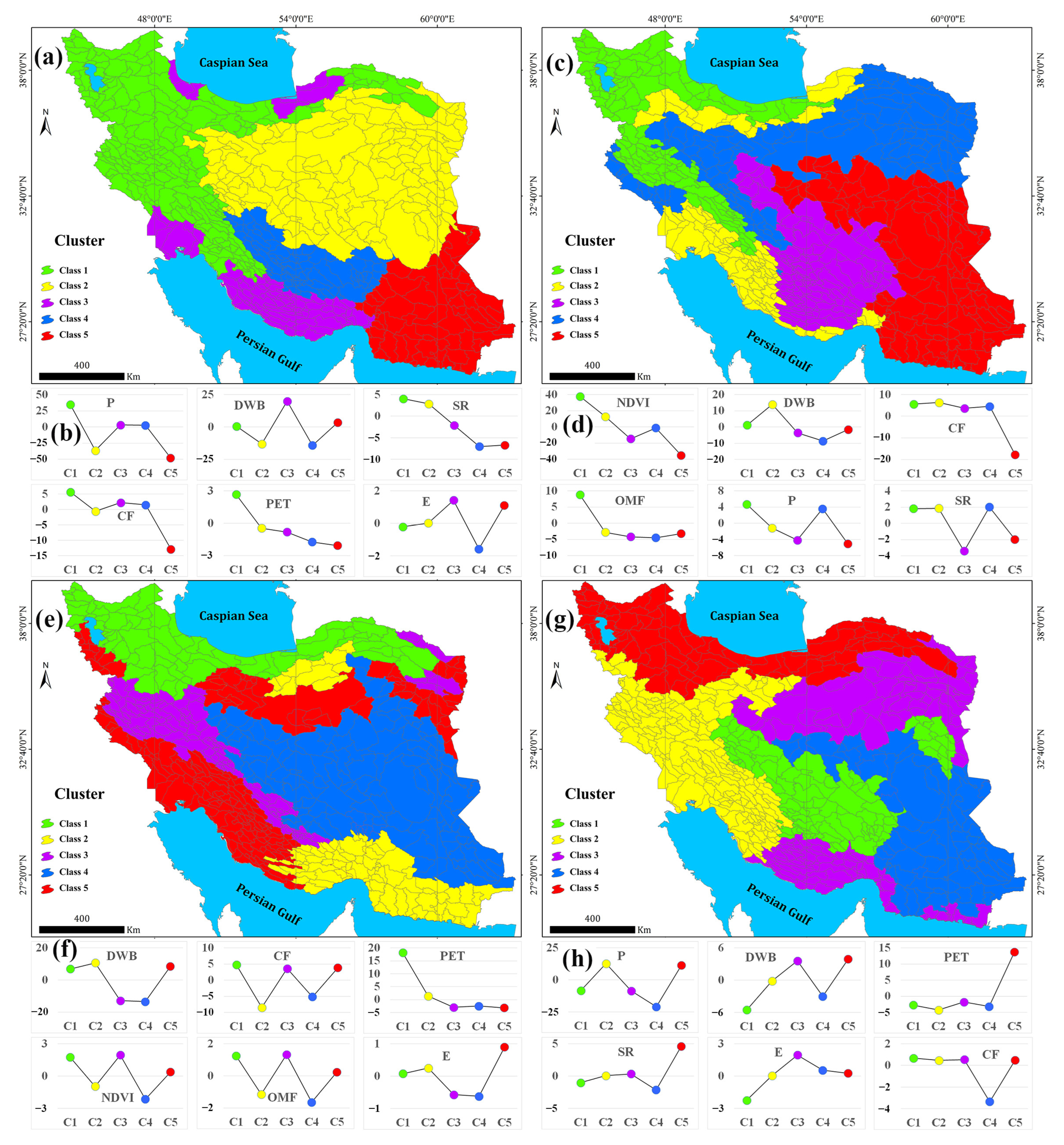
3.5. Cluster Analysis
4. Conclusions
Supplementary Materials
Author Contributions
Funding
Data Availability Statement
Acknowledgments
Conflicts of Interest
References
- Seneviratne, S.I.; Corti, T.; Davin, E.L.; Hirschi, M.; Jaeger, E.B.; Lehner, I.; Orlowsky, B.; Teuling, A.J. Investigating Soil Moisture–Climate Interactions in a Changing Climate: A Review. Earth-Sci. Rev. 2010, 99, 125–161. [Google Scholar] [CrossRef]
- Zhang, L.; Zeng, Y.; Zhuang, R.; Szabó, B.; Manfreda, S.; Han, Q.; Su, Z. In Situ Observation-Constrained Global Surface Soil Moisture Using Random Forest Model. Remote Sens. 2021, 13, 4893. [Google Scholar] [CrossRef]
- Han, Q.; Zeng, Y.; Zhang, L.; Wang, C.; Prikaziuk, E.; Niu, Z.; Su, B. Global Long Term Daily 1 Km Surface Soil Moisture Dataset with Physics Informed Machine Learning. Sci. Data 2023, 10, 101. [Google Scholar] [CrossRef] [PubMed]
- Sure, A.; Dikshit, O. Estimation of Root Zone Soil Moisture Using Passive Microwave Remote Sensing: A Case Study for Rice and Wheat Crops for Three States in the Indo-Gangetic Basin. J. Environ. Manag. 2019, 234, 75–89. [Google Scholar] [CrossRef] [PubMed]
- Yang, Q.; Fan, J.; Luo, Z. Response of Soil Moisture and Vegetation Growth to Precipitation under Different Land Uses in the Northern Loess Plateau, China. Catena 2024, 236, 107728. [Google Scholar] [CrossRef]
- Cosh, M.H.; Jackson, T.J.; Moran, S.; Bindlish, R. Temporal Persistence and Stability of Surface Soil Moisture in a Semi-Arid Watershed. Remote Sens. Environ. 2008, 112, 304–313. [Google Scholar] [CrossRef]
- Parizi, E.; Hosseini, S.M.; Ataie-Ashtiani, B.; Simmons, C.T. Normalized Difference Vegetation Index as the Dominant Predicting Factor of Groundwater Recharge in Phreatic Aquifers: Case Studies across Iran. Sci. Rep. 2020, 10, 17473. [Google Scholar] [CrossRef] [PubMed]
- D’Odorico, P.; Caylor, K.; Okin, G.S.; Scanlon, T.M. On Soil Moisture–Vegetation Feedbacks and Their Possible Effects on the Dynamics of Dryland Ecosystems. J. Geophys. Res. Biogeosci. 2007, 112, G04010. [Google Scholar] [CrossRef]
- Cai, Y.; Zheng, W.; Zhang, X.; Zhangzhong, L.; Xue, X. Research on Soil Moisture Prediction Model Based on Deep Learning. PLoS ONE 2019, 14, e0214508. [Google Scholar] [CrossRef] [PubMed]
- Lagos, M.; Serna, J.L.; Muñoz, J.F.; Suárez, F. Challenges in Determining Soil Moisture and Evaporation Fluxes Using Distributed Temperature Sensing Methods. J. Environ. Manag. 2020, 261, 110232. [Google Scholar] [CrossRef] [PubMed]
- Nikraftar, Z.; Mostafaie, A.; Sadegh, M.; Afkueieh, J.H.; Pradhan, B. Multi-Type Assessment of Global Droughts and Teleconnections. Weather Clim. Extrem. 2021, 34, 100402. [Google Scholar] [CrossRef]
- Gruber, A.; Dorigo, W.A.; Zwieback, S.; Xaver, A.; Wagner, W. Characterizing Coarse-Scale Representativeness of in Situ Soil Moisture Measurements from the International Soil Moisture Network. Vadose Zone J. 2013, 12, vzj2012-0170. [Google Scholar] [CrossRef]
- Everson, C.; Mengistu, M.; Vather, T. The Validation of the Variables (Evaporation and Soil Water) in Hydrometeorological Models: Phase II, Application of Cosmic Ray Probes for Soil Water Measurement. Water Res. Comm. Pretoria S. Afr. WRC Rep. 2017, 17, 4. Available online: https://www.wrc.org.za/wp-content/uploads/mdocs/2323-1-171.pdf (accessed on 17 July 2017).
- Rasheed, M.W.; Tang, J.; Sarwar, A.; Shah, S.; Saddique, N.; Khan, M.U.; Imran Khan, M.; Nawaz, S.; Shamshiri, R.R.; Aziz, M. Soil Moisture Measuring Techniques and Factors Affecting the Moisture Dynamics: A Comprehensive Review. Sustainability 2022, 14, 11538. [Google Scholar] [CrossRef]
- Xu, L.; Chen, N.; Zhang, X.; Moradkhani, H.; Zhang, C.; Hu, C. In-Situ and Triple-Collocation Based Evaluations of Eight Global Root Zone Soil Moisture Products. Remote Sens. Environ. 2021, 254, 112248. [Google Scholar] [CrossRef]
- Dorigo, W.; Himmelbauer, I.; Aberer, D.; Schremmer, L.; Petrakovic, I.; Zappa, L.; Preimesberger, W.; Xaver, A.; Annor, F.; Ardö, J. The International Soil Moisture Network: Serving Earth System Science for over a Decade. Hydrol. Earth Syst. Sci. Discuss. 2021, 2021, 1–83. [Google Scholar] [CrossRef]
- Jamei, M.; Mousavi Baygi, M.; Oskouei, E.A.; Lopez-Baeza, E. Validation of the SMOS Level 1C Brightness Temperature and Level 2 Soil Moisture Data over the West and Southwest of Iran. Remote Sens. 2020, 12, 2819. [Google Scholar] [CrossRef]
- Guevara, M.; Taufer, M.; Vargas, R. Gap-Free Global Annual Soil Moisture: 15 Km Grids for 1991–2018. Earth Syst. Sci. Data Discuss. 2020, 2020, 1–65. [Google Scholar] [CrossRef]
- Xu, L.; Chen, N.; Chen, Z.; Zhang, C.; Yu, H. Spatiotemporal Forecasting in Earth System Science: Methods, Uncertainties, Predictability and Future Directions. Earth-Sci. Rev. 2021, 222, 103828. [Google Scholar] [CrossRef]
- Cho, E.; Choi, M. Regional Scale Spatio-Temporal Variability of Soil Moisture and Its Relationship with Meteorological Factors over the Korean Peninsula. J. Hydrol. 2014, 516, 317–329. [Google Scholar] [CrossRef]
- Fu, X.; Jiang, X.; Yu, Z.; Ding, Y.; Lü, H.; Zheng, D. Understanding the Key Factors That Influence Soil Moisture Estimation Using the Unscented Weighted Ensemble Kalman Filter. Agric. For. Meteorol. 2022, 313, 108745. [Google Scholar] [CrossRef]
- Wang, T.; Franz, T.E. Field Observations of Regional Controls of Soil Hydraulic Properties on Soil Moisture Spatial Variability in Different Climate Zones. Vadose Zone J. 2015, 14, vzj2015-02. [Google Scholar] [CrossRef]
- Perry, M.A.; Niemann, J.D. Analysis and Estimation of Soil Moisture at the Catchment Scale Using EOFs. J. Hydrol. 2007, 334, 388–404. [Google Scholar] [CrossRef]
- Jiang, Z.; Huete, A.R.; Didan, K.; Miura, T. Development of a Two-Band Enhanced Vegetation Index without a Blue Band. Remote Sens. Environ. 2008, 112, 3833–3845. [Google Scholar] [CrossRef]
- Meng, F.; Luo, M.; Sa, C.; Wang, M.; Bao, Y. Quantitative Assessment of the Effects of Climate, Vegetation, Soil and Groundwater on Soil Moisture Spatiotemporal Variability in the Mongolian Plateau. Sci. Total Environ. 2022, 809, 152198. [Google Scholar] [CrossRef] [PubMed]
- Jung, M.; Reichstein, M.; Ciais, P.; Seneviratne, S.I.; Sheffield, J.; Goulden, M.L.; Bonan, G.; Cescatti, A.; Chen, J.; De Jeu, R. Recent Decline in the Global Land Evapotranspiration Trend Due to Limited Moisture Supply. Nature 2010, 467, 951–954. [Google Scholar] [CrossRef] [PubMed]
- de Queiroz, M.G.; da Silva, T.G.F.; Zolnier, S.; Jardim, A.M.d.R.F.; de Souza, C.A.A.; Júnior, G.D.N.A.; de Morais, J.E.F.; de Souza, L.S.B. Spatial and Temporal Dynamics of Soil Moisture for Surfaces with a Change in Land Use in the Semi-Arid Region of Brazil. Catena 2020, 188, 104457. [Google Scholar] [CrossRef]
- Wang, Y.; Yang, J.; Chen, Y.; Fang, G.; Duan, W.; Li, Y.; De Maeyer, P. Quantifying the Effects of Climate and Vegetation on Soil Moisture in an Arid Area, China. Water 2019, 11, 767. [Google Scholar] [CrossRef]
- Grayson, R.B.; Western, A.W.; Chiew, F.H.; Blöschl, G. Preferred States in Spatial Soil Moisture Patterns: Local and Nonlocal Controls. Water Resour. Res. 1997, 33, 2897–2908. [Google Scholar] [CrossRef]
- Boueshagh, M.; Hasanlou, M. Estimating Water Level in the Urmia Lake Using Satellite Data: A Machine Learning Approach. Int. Arch. Photogramm. Remote Sens. Spat. Inf. Sci. 2019, 42, 219–226. [Google Scholar] [CrossRef]
- Ahmad, S.; Kalra, A.; Stephen, H. Estimating Soil Moisture Using Remote Sensing Data: A Machine Learning Approach. Adv. Water Resour. 2010, 33, 69–80. [Google Scholar] [CrossRef]
- Tyralis, H.; Papacharalampous, G.; Langousis, A. A Brief Review of Random Forests for Water Scientists and Practitioners and Their Recent History in Water Resources. Water 2019, 11, 910. [Google Scholar] [CrossRef]
- Carranza, C.; Nolet, C.; Pezij, M.; van der Ploeg, M. Root Zone Soil Moisture Estimation with Random Forest. J. Hydrol. 2021, 593, 125840. [Google Scholar] [CrossRef]
- Wang, S.; Peng, H.; Liang, S. Prediction of Estuarine Water Quality Using Interpretable Machine Learning Approach. J. Hydrol. 2022, 605, 127320. [Google Scholar] [CrossRef]
- Lundberg, S.M.; Lee, S.-I. A Unified Approach to Interpreting Model Predictions. Adv. Neural Inf. Process. Syst. 2017, 30, 2. [Google Scholar] [CrossRef]
- Liu, Q.; Gui, D.; Zhang, L.; Niu, J.; Dai, H.; Wei, G.; Hu, B.X. Simulation of Regional Groundwater Levels in Arid Regions Using Interpretable Machine Learning Models. Sci. Total Environ. 2022, 831, 154902. [Google Scholar] [CrossRef] [PubMed]
- Nikraftar, Z.; Parizi, E.; Saber, M.; Hosseini, S.M.; Ataie-Ashtiani, B.; Simmons, C.T. Groundwater Sustainability Assessment in the Middle East Using GRACE/GRACE-FO Data. Hydrogeol. J. 2024, 32, 321–337. [Google Scholar] [CrossRef]
- Rahmani, A.; Golian, S.; Brocca, L. Multiyear Monitoring of Soil Moisture over Iran through Satellite and Reanalysis Soil Moisture Products. Int. J. Appl. Earth Obs. Geoinf. 2016, 48, 85–95. [Google Scholar] [CrossRef]
- IMO Iran Meteorological Organization. 2023. Available online: https://www.irimo.ir/index.php?newlang=eng (accessed on 17 July 2017).
- Ashraf, S.; Nazemi, A.; AghaKouchak, A. Anthropogenic Drought Dominates Groundwater Depletion in Iran. Sci. Rep. 2021, 11, 9135. [Google Scholar] [CrossRef] [PubMed]
- Sivakumar, M.V.K.; Stefanski, R. Climate and Land Degradation—An Overview. In Climate and Land Degradation; Sivakumar, M.V.K., Ndiang’ui, N., Eds.; Environmental Science and Engineering; Springer: Berlin/Heidelberg, Germany, 2007; pp. 105–135. ISBN 978-3-540-72437-7. [Google Scholar] [CrossRef]
- Gheybi, F.; Paridad, P.; Faridani, F.; Farid, A.; Pizarro, A.; Fiorentino, M.; Manfreda, S. Soil Moisture Monitoring in Iran by Implementing Satellite Data into the Root-Zone SMAR Model. Hydrology 2019, 6, 44. [Google Scholar] [CrossRef]
- Saadatabadi, A.R.; Izadi, N.; Karakani, E.G.; Fattahi, E.; Shamsipour, A.A. Investigating Relationship between Soil Moisture, Hydro-Climatic Parameters, Vegetation, and Climate Change Impacts in a Semi-Arid Basin in Iran. Arab. J. Geosci. 2021, 14, 1796. [Google Scholar] [CrossRef]
- IWRMC Iran Water Resources Management Company. 2023. Available online: https://www.wrm.ir/?l=EN (accessed on 17 July 2017).
- ESA-WorldCover Worldwide Land Cover Mapping. 2020. Available online: https://esa-worldcover.org/en (accessed on 17 July 2017).
- Hossein-Panahi, B.; Golestani, A.; Amani, K.; Hosseini, S.M.; Parizi, E. Suspended Sediment Yield Estimation Using Geomorphologic Instantaneous Unit Sedimentgraph: A Case Study from the Southern Caspian Sea Iran. Int. J. River Basin Manag. 2024, 1–13. [Google Scholar] [CrossRef]
- Colliander, A.; Cosh, M.H.; Misra, S.; Jackson, T.J.; Crow, W.T.; Chan, S.; Bindlish, R.; Chae, C.; Collins, C.H.; Yueh, S.H. Validation and Scaling of Soil Moisture in a Semi-Arid Environment: SMAP Validation Experiment 2015 (SMAPVEX15). Remote Sens. Environ. 2017, 196, 101–112. [Google Scholar] [CrossRef]
- Tian, J.; Zhang, Y. Comprehensive Validation of Seven Root Zone Soil Moisture Products at 1153 Ground Sites across China. Int. J. Digit. Earth 2023, 16, 4008–4022. [Google Scholar] [CrossRef]
- Wu, X.; Lu, G.; Wu, Z.; He, H.; Scanlon, T.; Dorigo, W. Triple Collocation-Based Assessment of Satellite Soil Moisture Products with in Situ Measurements in China: Understanding the Error Sources. Remote Sens. 2020, 12, 2275. [Google Scholar] [CrossRef]
- Kimball, J.; Jones, L.; Glassy, J.; Reichle, R. SMAP L4 Global Daily 9 Km Carbon Net Ecosystem Exchange, Version 2; NASA National Snow and Ice Data Center Distributed Active Archive Center (DAAC) Data Set; National Snow and Ice Data Center: Boulder, CO, USA, 2016. [Google Scholar] [CrossRef]
- Reichle, R.H.; Liu, Q.; Koster, R.D.; Crow, W.T.; De Lannoy, G.J.; Kimball, J.S.; Ardizzone, J.V.; Bosch, D.; Colliander, A.; Cosh, M. Version 4 of the SMAP Level-4 Soil Moisture Algorithm and Data Product. J. Adv. Model. Earth Syst. 2019, 11, 3106–3130. [Google Scholar] [CrossRef]
- Kimball, J.; Jones, L.; Endsley, A.; Kundig, T.; Reichle, R. SMAP L4 Global Daily 9 Km EASE-Grid Carbon Net Ecosystem Exchange, Version 4; National Snow and Ice Data Center: Boulder, CO, USA, 2018. [Google Scholar] [CrossRef]
- Gelaro, R.; McCarty, W.; Suárez, M.J.; Todling, R.; Molod, A.; Takacs, L.; Randles, C.A.; Darmenov, A.; Bosilovich, M.G.; Reichle, R. The Modern-Era Retrospective Analysis for Research and Applications, Version 2 (MERRA-2). J. Clim. 2017, 30, 5419–5454. [Google Scholar] [CrossRef] [PubMed]
- Saha, S.; Tripp, P. CFSv2 Retrospective Forecasts; NOAA/NWS/NCEP Environmental Modeling Center Tech. Rep: College Park, Maryland, 2011. Available online: https://www.cpc.ncep.noaa.gov/products/CFSv2/CFSv2_body.html (accessed on 17 July 2017).
- Reichle, R.H.; Draper, C.S.; Liu, Q.; Girotto, M.; Mahanama, S.P.; Koster, R.D.; De Lannoy, G.J. Assessment of MERRA-2 Land Surface Hydrology Estimates. J. Clim. 2017, 30, 2937–2960. [Google Scholar] [CrossRef]
- Saha, S.; Moorthi, S.; Wu, X.; Wang, J.; Nadiga, S.; Tripp, P.; Behringer, D.; Hou, Y.-T.; Chuang, H.; Iredell, M. The NCEP Climate Forecast System Version 2. J. Clim. 2014, 27, 2185–2208. [Google Scholar] [CrossRef]
- Dirmeyer, P.A.; Halder, S. Sensitivity of Numerical Weather Forecasts to Initial Soil Moisture Variations in CFSv2. Weather Forecast. 2016, 31, 1973–1983. [Google Scholar] [CrossRef]
- Patel, N.; Anapashsha, R.; Kumar, S.; Saha, S.; Dadhwal, V. Assessing Potential of MODIS Derived Temperature/Vegetation Condition Index (TVDI) to Infer Soil Moisture Status. Int. J. Remote Sens. 2009, 30, 23–39. [Google Scholar] [CrossRef]
- Zhao, W.; Sánchez, N.; Lu, H.; Li, A. A Spatial Downscaling Approach for the SMAP Passive Surface Soil Moisture Product Using Random Forest Regression. J. Hydrol. 2018, 563, 1009–1024. [Google Scholar] [CrossRef]
- Du Toit, W. Radial Basis Function Interpolation. 2008. Available online: https://scholar.sun.ac.za/handle/10019.1/2002 (accessed on 17 July 2017).
- Running, S.; Mu, Q.; Zhao, M. Mod16a2 Modis/Terra Net Evapotranspiration 8-Day L4 Global 500m Sin Grid V006. 2017. Available online: https://ladsweb.modaps.eosdis.nasa.gov/missions-and-measurements/products/MOD16A2 (accessed on 17 July 2017).
- Muñoz-Sabater, J.; Dutra, E.; Agustí-Panareda, A.; Albergel, C.; Arduini, G.; Balsamo, G.; Boussetta, S.; Choulga, M.; Harrigan, S.; Hersbach, H. ERA5-Land: A State-of-the-Art Global Reanalysis Dataset for Land Applications. Earth Syst. Sci. Data 2021, 13, 4349–4383. [Google Scholar] [CrossRef]
- Hossein-Panahi, B.; Samani, S.M.; Sadeghi, A.-R.; Shahi, M.; Hosseini, S.M.; Parizi, E. River Baseflow in Supplying Reservoirs Inflows of Tehran Metropolis: A Machine Learning Modeling Based on Influencing Factors. J. Hydrol. Reg. Stud. 2025, 60, 102528. [Google Scholar] [CrossRef]
- European Space Agency (ESA). Google. Harmonized Sentinel-2 MSI: MultiSpectral Instrument, Level-2A (Surface Reflectance) [COPERNICUS/S2_SR_HARMONIZED]. 2023. Available online: https://developers.google.com/earth-engine/datasets/catalog/COPERNICUS_S2_SR_HARMONIZED (accessed on 14 September 2024).
- National Oceanic and Atmospheric Administration Ocean and Coasts 2024. Available online: https://www.noaa.gov/ocean-coasts (accessed on 17 July 2017).
- Hengl, T.; Mendes De Jesus, J.; Heuvelink, G.B.M.; Ruiperez Gonzalez, M.; Kilibarda, M.; Blagotić, A.; Shangguan, W.; Wright, M.N.; Geng, X.; Bauer-Marschallinger, B.; et al. SoilGrids250m: Global Gridded Soil Information Based on Machine Learning. PLoS ONE 2017, 12, e0169748. [Google Scholar] [CrossRef] [PubMed]
- Tadono, T.; Nagai, H.; Ishida, H.; Oda, F.; Naito, S.; Minakawa, K.; Iwamoto, H. Generation of the 30 M-Mesh Global Digital Surface Model by ALOS PRISM. Int. Arch. Photogramm. Remote Sens. Spat. Inf. Sci. 2016, 41, 157–162. [Google Scholar] [CrossRef]
- ESRI Spatial Analysis. 2013. Available online: https://www.esri.com/en-us/home (accessed on 17 July 2017).
- Amani, M.; Ghorbanian, A.; Ahmadi, S.A.; Kakooei, M.; Moghimi, A.; Mirmazloumi, S.M.; Moghaddam, S.H.A.; Mahdavi, S.; Ghahremanloo, M.; Parsian, S. Google Earth Engine Cloud Computing Platform for Remote Sensing Big Data Applications: A Comprehensive Review. IEEE J. Sel. Top. Appl. Earth Obs. Remote Sens. 2020, 13, 5326–5350. [Google Scholar] [CrossRef]
- Tang, G.; Clark, M.P.; Papalexiou, S.M.; Ma, Z.; Hong, Y. Have Satellite Precipitation Products Improved over Last Two Decades? A Comprehensive Comparison of GPM IMERG with Nine Satellite and Reanalysis Datasets. Remote Sens. Environ. 2020, 240, 111697. [Google Scholar] [CrossRef]
- Saemian, P.; Hosseini-Moghari, S.-M.; Fatehi, I.; Shoarinezhad, V.; Modiri, E.; Tourian, M.J.; Tang, Q.; Nowak, W.; Bárdossy, A.; Sneeuw, N. Comprehensive Evaluation of Precipitation Datasets over Iran. J. Hydrol. 2021, 603, 127054. [Google Scholar] [CrossRef]
- Fahrudin, T.; Wijaya, D.R.; Agung, A.A.G. COVID-19 Confirmed Case Correlation Analysis Based on Spearman and Kendall Correlation. In Proceedings of the 2020 International Conference on Data Science and Its Applications (ICoDSA), Bandung, Indonesia, 5–6 August 2020; pp. 1–4. [Google Scholar] [CrossRef]
- Parizi, E.; Khojeh, S.; Hosseini, S.M.; Moghadam, Y.J. Application of Unmanned Aerial Vehicle DEM in Flood Modeling and Comparison with Global DEMs: Case Study of Atrak River Basin, Iran. J. Environ. Manag. 2022, 317, 115492. [Google Scholar] [CrossRef] [PubMed]
- Gupta, H.V.; Kling, H.; Yilmaz, K.K.; Martinez, G.F. Decomposition of the Mean Squared Error and NSE Performance Criteria: Implications for Improving Hydrological Modelling. J. Hydrol. 2009, 377, 80–91. [Google Scholar] [CrossRef]
- Kling, H.; Fuchs, M.; Paulin, M. Runoff Conditions in the Upper Danube Basin under an Ensemble of Climate Change Scenarios. J. Hydrol. 2012, 424, 264–277. [Google Scholar] [CrossRef]
- Naghibi, S.A.; Pourghasemi, H.R.; Dixon, B. GIS-Based Groundwater Potential Mapping Using Boosted Regression Tree, Classification and Regression Tree, and Random Forest Machine Learning Models in Iran. Environ. Monit. Assess. 2016, 188, 44. [Google Scholar] [CrossRef] [PubMed]
- Breiman, L.; Cutler, A. State of the Art of Data Mining Using Random Forest. In Proceedings of the Salford Data Mining Conference, San Diego, CA, USA, 24–25 May 2012; pp. 24–25. [Google Scholar] [CrossRef]
- Pouyan, S.; Pourghasemi, H.R.; Bordbar, M.; Rahmanian, S.; Clague, J.J. A Multi-Hazard Map-Based Flooding, Gully Erosion, Forest Fires, and Earthquakes in Iran. Sci. Rep. 2021, 11, 14889. [Google Scholar] [CrossRef] [PubMed]
- Kaiser, M.; Günnemann, S.; Disse, M. Regional-Scale Prediction of Pluvial and Flash Flood Susceptible Areas Using Tree-Based Classifiers. J. Hydrol. 2022, 612, 128088. [Google Scholar] [CrossRef]
- Amini, S.; Saber, M.; Rabiei-Dastjerdi, H.; Homayouni, S. Urban Land Use and Land Cover Change Analysis Using Random Forest Classification of Landsat Time Series. Remote Sens. 2022, 14, 2654. [Google Scholar] [CrossRef]
- Pedregosa, F.; Varoquaux, G.; Gramfort, A.; Michel, V.; Thirion, B.; Grisel, O.; Blondel, M.; Prettenhofer, P.; Weiss, R.; Dubourg, V. Scikit-Learn: Machine Learning in Python. J. Mach. Learn. Res. 2011, 12, 2825–2830. [Google Scholar]
- Buitinck, L.; Louppe, G.; Blondel, M.; Pedregosa, F.; Mueller, A.; Grisel, O.; Niculae, V.; Prettenhofer, P.; Gramfort, A.; Grobler, J. API Design for Machine Learning Software: Experiences from the Scikit-Learn Project. arXiv 2013, arXiv:1309.0238. [Google Scholar]
- Aksu, G.; Güzeller, C.O.; Eser, M.T. The Effect of the Normalization Method Used in Different Sample Sizes on the Success of Artificial Neural Network Model. Int. J. Assess. Tools Educ. 2019, 6, 170–192. [Google Scholar] [CrossRef]
- Van den Broeck, G.; Lykov, A.; Schleich, M.; Suciu, D. On the Tractability of SHAP Explanations. J. Artif. Intell. Res. 2022, 74, 851–886. [Google Scholar] [CrossRef]
- Başağaoğlu, H.; Chakraborty, D.; Lago, C.D.; Gutierrez, L.; Şahinli, M.A.; Giacomoni, M.; Furl, C.; Mirchi, A.; Moriasi, D.; Şengör, S.S. A Review on Interpretable and Explainable Artificial Intelligence in Hydroclimatic Applications. Water 2022, 14, 1230. [Google Scholar] [CrossRef]
- Zhang, B.; Salem, F.K.A.; Hayes, M.J.; Smith, K.H.; Tadesse, T.; Wardlow, B.D. Explainable Machine Learning for the Prediction and Assessment of Complex Drought Impacts. Sci. Total Environ. 2023, 898, 165509. [Google Scholar] [CrossRef] [PubMed]
- Kanani-Sadat, Y.; Safari, A.; Nasseri, M.; Homayouni, S. A Novel Explainable PSO-XGBoost Model for Regional Flood Frequency Analysis at a National Scale: Exploring Spatial Heterogeneity in Flood Drivers. J. Hydrol. 2024, 638, 131493. [Google Scholar] [CrossRef]
- Ye, S.; Chai, Y.; Li, J.; Wang, J.; Deng, X.; Ran, Q. Explainable Transfer Learning for Subsurface Soil Moisture Prediction. J. Hydrol. 2025, 661, 133473. [Google Scholar] [CrossRef]
- Hu, L.; Wang, K. Computing SHAP Efficiently Using Model Structure Information. arXiv 2023. [Google Scholar] [CrossRef]
- Yang, J. Fast TreeSHAP: Accelerating SHAP Value Computation for Trees. arXiv 2021. [Google Scholar] [CrossRef]
- Hiabu, M.; Meyer, J.T.; Wright, M.N. Unifying Local and Global Model Explanations by Functional Decomposition of Low Dimensional Structures. arXiv 2022. [Google Scholar] [CrossRef]
- Chiu, T.; Fang, D.; Chen, J.; Wang, Y.; Jeris, C. A Robust and Scalable Clustering Algorithm for Mixed Type Attributes in Large Database Environment. In Proceedings of the Seventh ACM SIGKDD International Conference on Knowledge Discovery and Data Minin, San Francisco, CA, USA, 26–29 August 2001; pp. 263–268. [Google Scholar] [CrossRef]
- Wu, X.; Benjamin Zhan, F.; Zhang, K.; Deng, Q. Application of a Two-Step Cluster Analysis and the Apriori Algorithm to Classify the Deformation States of Two Typical Colluvial Landslides in the Three Gorges, China. Environ. Earth Sci. 2016, 75, 146. [Google Scholar] [CrossRef]
- Fahy, B.; Brenneman, E.; Chang, H.; Shandas, V. Spatial Analysis of Urban Flooding and Extreme Heat Hazard Potential in Portland, OR. Int. J. Disaster Risk Reduct. 2019, 39, 101117. [Google Scholar] [CrossRef]
- Qin, H.; Huang, Q.; Zhang, Z.; Lu, Y.; Li, M.; Xu, L.; Chen, Z. Carbon Dioxide Emission Driving Factors Analysis and Policy Implications of Chinese Cities: Combining Geographically Weighted Regression with Two-Step Cluster. Sci. Total Environ. 2019, 684, 413–424. [Google Scholar] [CrossRef] [PubMed]
- Satish, S.; Bharadhwaj, S. Information Search Behaviour among New Car Buyers: A Two-Step Cluster Analysis. IIMB Manag. Rev. 2010, 22, 5–15. [Google Scholar] [CrossRef]
- Chen, F.; Crow, W.T.; Bindlish, R.; Colliander, A.; Burgin, M.S.; Asanuma, J.; Aida, K. Global-Scale Evaluation of SMAP, SMOS and ASCAT Soil Moisture Products Using Triple Collocation. Remote Sens. Environ. 2018, 214, 1–13. [Google Scholar] [CrossRef] [PubMed]
- Maleki, K.H.; Vaezi, A.R.; Sarmadian, F.; Crow, W.T. Validation of Satellite-Based Soil Moisture Retrievals from SMAP with in Situ Observation in the Simineh-Zarrineh (Bokan) Catchment, NW of Iran. Eurasian J. Soil Sci. 2019, 8, 340–350. [Google Scholar] [CrossRef]
- Saeedi, M.; Sharafati, A.; Tavakol, A. Evaluation of Gridded Soil Moisture Products over Varied Land Covers, Climates, and Soil Textures Using in Situ Measurements: A Case Study of Lake Urmia Basin. Theor. Appl. Climatol. 2021, 145, 1053–1074. [Google Scholar] [CrossRef]
- Jamei, M.; Lopez-Baeza, E.; Asadi, E. Validation of SMAP Surface Soil Moisture Products over Iran. In Proceedings of the 44th COSPAR Sci. Assembly, Athens, Greece, 16–24 July 2022; Volume 44, p. 123. Available online: https://ui.adsabs.harvard.edu/abs/2022cosp...44..123J/abstract (accessed on 17 July 2017).
- Amini, A.; Moghadam, M.K.; Kolahchi, A.A.; Raheli-Namin, M.; Ahmed, K.O. Evaluation of GLDAS Soil Moisture Product over Kermanshah Province, Iran. H2Open J. 2023, 6, 373–386. [Google Scholar] [CrossRef]
- Fakharizadehshirazi, E.; Sabziparvar, A.A.; Sodoudi, S. Long-Term Spatiotemporal Variations in Satellite-Based Soil Moisture and Vegetation Indices over Iran. Environ. Earth Sci. 2019, 78, 342. [Google Scholar] [CrossRef]
- Garcia-Estringana, P.; Latron, J.; Llorens, P.; Gallart, F. Spatial and Temporal Dynamics of Soil Moisture in a Mediterranean Mountain Area (Vallcebre, NE Spain). Ecohydrology 2013, 6, 741–753. [Google Scholar] [CrossRef]
- Jin, Z.; Guo, L.; Lin, H.; Wang, Y.; Yu, Y.; Chu, G.; Zhang, J. Soil Moisture Response to Rainfall on the Chinese Loess Plateau after a Long-term Vegetation Rehabilitation. Hydrol. Process. 2018, 32, 1738–1754. [Google Scholar] [CrossRef]
- Feng, T.; Shen, Y.; Wang, F.; Chen, Q.; Ji, K. Spatiotemporal Variability and Driving Factors of the Shallow Soil Moisture in North China during the Past 31 Years. J. Hydrol. 2023, 619, 129331. [Google Scholar] [CrossRef]
- Zhou, Q.; Sun, Z.; Liu, X.; Wei, X.; Peng, Z.; Yue, C.; Luo, Y. Temporal Soil Moisture Variations in Different Vegetation Cover Types in Karst Areas of Southwest China: A Plot Scale Case Study. Water 2019, 11, 1423. [Google Scholar] [CrossRef]
- Janani, N.; Kannan, B.; Nagarajan, K.; Thiyagarajan, G.; Duraisamy, M.R. Soil Moisture Mapping for Different Land-Use Patterns of Lower Bhavani River Basin Using Vegetative Index and Land Surface Temperature. Env. Dev Sustain 2023, 26, 4533–4549. [Google Scholar] [CrossRef]
- Nikraftar, Z.; Parizi, E.; Hosseini, S.M.; Ataie-Ashtiani, B. Lake Urmia Restoration Success Story: A Natural Trend or a Planned Remedy? J. Great Lakes Res. 2021, 47, 955–969. [Google Scholar] [CrossRef]
- Khosravi, K.; Panahi, M.; Golkarian, A.; Keesstra, S.D.; Saco, P.M.; Bui, D.T.; Lee, S. Convolutional Neural Network Approach for Spatial Prediction of Flood Hazard at National Scale of Iran. J. Hydrol. 2020, 591, 125552. [Google Scholar] [CrossRef]
- Sadeghi, M.; Shearer, E.J.; Mosaffa, H.; Gorooh, V.A.; Naeini, M.R.; Hayatbini, N.; Katiraie-Boroujerdy, P.-S.; Analui, B.; Nguyen, P.; Sorooshian, S. Application of Remote Sensing Precipitation Data and the CONNECT Algorithm to Investigate Spatiotemporal Variations of Heavy Precipitation: Case Study of Major Floods across Iran (Spring 2019). J. Hydrol. 2021, 600, 126569. [Google Scholar] [CrossRef]
- Adab, H.; Morbidelli, R.; Saltalippi, C.; Moradian, M.; Ghalhari, G.A.F. Machine Learning to Estimate Surface Soil Moisture from Remote Sensing Data. Water 2020, 12, 3223. [Google Scholar] [CrossRef]
- Fathololoumi, S.; Vaezi, A.R.; Alavipanah, S.K.; Ghorbani, A.; Biswas, A. Comparison of Spectral and Spatial-Based Approaches for Mapping the Local Variation of Soil Moisture in a Semi-Arid Mountainous Area. Sci. Total Environ. 2020, 724, 138319. [Google Scholar] [CrossRef] [PubMed]
- Choubin, B.; Darabi, H.; Rahmati, O.; Sajedi-Hosseini, F.; Kløve, B. River Suspended Sediment Modelling Using the CART Model: A Comparative Study of Machine Learning Techniques. Sci. Total Environ. 2018, 615, 272–281. [Google Scholar] [CrossRef] [PubMed]
- Ekmekcioğlu, Ö.; Koc, K.; Özger, M.; Işık, Z. Exploring the Additional Value of Class Imbalance Distributions on Interpretable Flash Flood Susceptibility Prediction in the Black Warrior River Basin, Alabama, United States. J. Hydrol. 2022, 610, 127877. [Google Scholar] [CrossRef]
- Tabari, H.; Talaee, P.H. Temporal Variability of Precipitation over Iran: 1966–2005. J. Hydrol. 2011, 396, 313–320. [Google Scholar] [CrossRef]
- Javari, M. Trend and Homogeneity Analysis of Precipitation in Iran. Climate 2016, 4, 44. [Google Scholar] [CrossRef]
- Feng, H.; Liu, Y. Combined Effects of Precipitation and Air Temperature on Soil Moisture in Different Land Covers in a Humid Basin. J. Hydrol. 2015, 531, 1129–1140. [Google Scholar] [CrossRef]
- Rascón-Ramos, A.E.; Martínez-Salvador, M.; Sosa-Pérez, G.; Villarreal-Guerrero, F.; Pinedo-Alvarez, A.; Santellano-Estrada, E.; Corrales-Lerma, R. Soil Moisture Dynamics in Response to Precipitation and Thinning in a Semi-Dry Forest in Northern Mexico. Water 2021, 13, 105. [Google Scholar] [CrossRef]
- Du, M.; Zhang, J.; Elmahdi, A.; Wang, Z.; Yang, Q.; Liu, H.; Liu, C.; Hu, Y.; Gu, N.; Bao, Z. Variation Characteristics and Influencing Factors of Soil Moisture Content in the Lime Concretion Black Soil Region in Northern Anhui. Water 2021, 13, 2251. [Google Scholar] [CrossRef]
- Wenwu, Z.; Xuening, F.; Daryanto, S.; Zhang, X.; Yaping, W. Factors Influencing Soil Moisture in the Loess Plateau, China: A Review. Earth Environ. Sci. Trans. R. Soc. Edinb. 2018, 109, 501–509. [Google Scholar] [CrossRef]
- Cai, J.; Zhou, B.; Chen, S.; Wang, X.; Yang, S.; Cheng, Z.; Wang, F.; Mei, X.; Wu, D. Spatial and Temporal Variability of Soil Moisture and Its Driving Factors in the Northern Agricultural Regions of China. Water 2024, 16, 556. [Google Scholar] [CrossRef]
- Yin, D.; Song, X.; Zhu, X.; Guo, H.; Zhang, Y.; Zhang, Y. Spatiotemporal Analysis of Soil Moisture Variability and Its Driving Factor. Remote Sens. 2023, 15, 5768. [Google Scholar] [CrossRef]
- Vachaud, G.; Passerat de Silans, A.; Balabanis, P.; Vauclin, M. Temporal Stability of Spatially Measured Soil Water Probability Density Function. Soil Sci. Soc. Am. J. 1985, 49, 822–828. [Google Scholar] [CrossRef]
- Ojha, R.; Morbidelli, R.; Saltalippi, C.; Flammini, A.; Govindaraju, R.S. Scaling of Surface Soil Moisture over Heterogeneous Fields Subjected to a Single Rainfall Event. J. Hydrol. 2014, 516, 21–36. [Google Scholar] [CrossRef]
- Li, Y.-X.; Leng, P.; Kasim, A.A.; Li, Z.-L. Spatiotemporal Variability and Dominant Driving Factors of Satellite Observed Global Soil Moisture from 2001 to 2020. J. Hydrol. 2025, 654, 132848. [Google Scholar] [CrossRef]
- Zhu, P.; Jia, X.; Zhao, C.; Shao, M. Long-Term Soil Moisture Evolution and Its Driving Factors across China’s Agroecosystems. Agric. Water Manag. 2022, 269, 107735. [Google Scholar] [CrossRef]
- Pellet, C.; Hauck, C. Monitoring Soil Moisture from Middle to High Elevation in Switzerland: Set-up and First Results from the SOMOMOUNT Network. Hydrol. Earth Syst. Sci. 2017, 21, 3199–3220. [Google Scholar] [CrossRef]
- Xu, M.; Xu, G.; Cheng, Y.; Min, Z.; Li, P.; Zhao, B.; Shi, P.; Xiao, L. Soil Moisture Estimation and Its Influencing Factors Based on Temporal Stability on a Semiarid Sloped Forestland. Front. Earth Sci. 2021, 9, 629826. [Google Scholar] [CrossRef]
- Vanderlinden, K.; Vereecken, H.; Hardelauf, H.; Herbst, M.; Martínez, G.; Cosh, M.H.; Pachepsky, Y.A. Temporal Stability of Soil Water Contents: A Review of Data and Analyses. Vadose Zone J. 2012, 11, vzj2011-0178. [Google Scholar] [CrossRef]
- Ghasemloo, N.; Matkan, A.A.; Alimohammadi, A.; Aghighi, H.; Mirbagheri, B. Estimating the Agricultural Farm Soil Moisture Using Spectral Indices of Landsat 8, and Sentinel-1, and Artificial Neural Networks. J. Geovisualization Spat. Anal. 2022, 6, 19. [Google Scholar] [CrossRef]
- Li, M.; Yan, Y. Comparative Analysis of Machine-Learning Models for Soil Moisture Estimation Using High-Resolution Remote-Sensing Data. Land 2024, 13, 1331. [Google Scholar] [CrossRef]
- Majdar, H.A.; Vafakhah, M.; Sharifikia, M.; Ghorbani, A. Spatial and Temporal Variability of Soil Moisture in Relation with Topographic and Meteorological Factors in South of Ardabil Province, Iran. Environ. Monit. Assess. 2018, 190, 500. [Google Scholar] [CrossRef] [PubMed]
- Bandak, S.; Boali, A.; Yaghobi, S.; Taghizadeh-Mehrjardi, R. Ensemble Machine Learning Approaches for Estimating Soil Texture Components in Loess Soils of Golestan Province. Earth Sci. Inform. 2025, 18, 396. [Google Scholar] [CrossRef]
- Laity, J.J. Deserts and Desert Environments; John Wiley & Sons: Hoboken, NJ, USA, 2009; Volume 3, ISBN 1-4443-0074-1. Available online: https://www.wiley.com/en-us/Deserts+and+Desert+Environments-p-9781444300741 (accessed on 17 July 2017).
- Parizi, E.; Hosseini, S.M.; Ataie-Ashtiani, B.; Simmons, C.T. Representative Pumping Wells Network to Estimate Groundwater Withdrawal from Aquifers: Lessons from a Developing Country, Iran. J. Hydrol. 2019, 578, 124090. [Google Scholar] [CrossRef]
- Goward, S.N.; Markham, B.; Dye, D.G.; Dulaney, W.; Yang, J. Normalized Difference Vegetation Index Measurements from the Advanced Very High Resolution Radiometer. Remote Sens. Environ. 1991, 35, 257–277. [Google Scholar] [CrossRef]
- Chen, X.; Hu, Q. Groundwater Influences on Soil Moisture and Surface Evaporation. J. Hydrol. 2004, 297, 285–300. [Google Scholar] [CrossRef]
- Fan, Y.; Li, H.; Miguez-Macho, G. Global Patterns of Groundwater Table Depth. Science 2013, 339, 940–943. [Google Scholar] [CrossRef] [PubMed]


| Number of Clusters | BIC | |||
|---|---|---|---|---|
| Winter | Spring | Summer | Autumn | |
| 1 | 2607 | 2607 | 2607 | 2607 |
| 2 | 2173 | 1952 | 2012 | 2059 |
| 3 | 1959 | 1706 | 1753 | 1707 |
| 4 | 1803 | 1594 | 1579 | 1514 |
| 5 | 1549 | 1432 | 1320 | 1268 |
| 6 | 1546 | 1428 | 1330 | 1260 |
| 7 | 1549 | 1432 | 1345 | 1291 |
| 8 | 1573 | 1440 | 1384 | 1328 |
| 9 | 1602 | 1453 | 1425 | 1378 |
| 10 | 1638 | 1480 | 1467 | 1428 |
| Season | Class | P | DWB | SR | CF | PET | E |
|---|---|---|---|---|---|---|---|
| Winter | 1 | 34.79 | 0.61 | 4.05 | 5.63 | 2.67 | −0.21 |
| 2 | −36.45 | −13.00 | 2.87 | −0.59 | −0.45 | 0.02 | |
| 3 | 3.19 | 19.96 | −2.10 | 2.19 | −0.81 | 1.42 | |
| 4 | 2.57 | −14.18 | −7.06 | 1.45 | −1.73 | −1.58 | |
| 5 | −47.93 | 3.53 | −6.71 | −12.87 | −2.06 | 1.11 | |
| NDVI | DWB | CF | OMF | P | SR | ||
| Spring | 1 | 37.69 | 1.15 | 5.63 | 8.79 | 4.71 | 1.82 |
| 2 | 12.72 | 13.93 | 6.31 | −2.80 | −1.18 | 1.85 | |
| 3 | −14.65 | −3.57 | 3.69 | −4.19 | −4.17 | −3.42 | |
| 4 | −1.35 | −8.68 | 4.55 | −4.46 | 3.58 | 2.02 | |
| 5 | −35.12 | −1.56 | −17.79 | −3.20 | −5.07 | −1.97 | |
| DWB | CF | PET | NDVI | OMF | E | ||
| Summer | 1 | 6.92 | 4.72 | 18.13 | 1.77 | 1.26 | 0.08 |
| 2 | 10.63 | −8.47 | 1.32 | −0.95 | −1.14 | 0.25 | |
| 3 | −12.85 | 3.59 | −3.01 | 1.96 | 1.32 | −0.57 | |
| 4 | −13.4 | −5.15 | −2.50 | −2.14 | −1.64 | −0.62 | |
| 5 | 8.47 | 3.83 | −3.15 | 0.38 | 0.24 | 0.90 | |
| P | DWB | PET | SR | E | CF | ||
| Autumn | 1 | −8.40 | −5.55 | −2.73 | −1.03 | −2.25 | 0.68 |
| 2 | 12.68 | −0.15 | −4.29 | 0.07 | 0.04 | 0.47 | |
| 3 | −8.54 | 3.59 | −1.83 | 0.34 | 1.96 | 0.54 | |
| 4 | −20.97 | −3.00 | −3.21 | −2.15 | 0.55 | −3.35 | |
| 5 | 11.52 | 3.92 | 13.74 | 4.62 | 0.26 | 0.49 | |
Disclaimer/Publisher’s Note: The statements, opinions and data contained in all publications are solely those of the individual author(s) and contributor(s) and not of MDPI and/or the editor(s). MDPI and/or the editor(s) disclaim responsibility for any injury to people or property resulting from any ideas, methods, instructions or products referred to in the content. |
© 2025 by the authors. Licensee MDPI, Basel, Switzerland. This article is an open access article distributed under the terms and conditions of the Creative Commons Attribution (CC BY) license (https://creativecommons.org/licenses/by/4.0/).
Share and Cite
Nikraftar, Z.; Parizi, E.; Saber, M.; Boueshagh, M.; Tavakoli, M.; Esmaeili Mahmoudabadi, A.; Ekradi, M.H.; Mbuvha, R.; Hosseini, S.M. An Interpretable Machine Learning Framework for Unraveling the Dynamics of Surface Soil Moisture Drivers. Remote Sens. 2025, 17, 2505. https://doi.org/10.3390/rs17142505
Nikraftar Z, Parizi E, Saber M, Boueshagh M, Tavakoli M, Esmaeili Mahmoudabadi A, Ekradi MH, Mbuvha R, Hosseini SM. An Interpretable Machine Learning Framework for Unraveling the Dynamics of Surface Soil Moisture Drivers. Remote Sensing. 2025; 17(14):2505. https://doi.org/10.3390/rs17142505
Chicago/Turabian StyleNikraftar, Zahir, Esmaeel Parizi, Mohsen Saber, Mahboubeh Boueshagh, Mortaza Tavakoli, Abazar Esmaeili Mahmoudabadi, Mohammad Hassan Ekradi, Rendani Mbuvha, and Seiyed Mossa Hosseini. 2025. "An Interpretable Machine Learning Framework for Unraveling the Dynamics of Surface Soil Moisture Drivers" Remote Sensing 17, no. 14: 2505. https://doi.org/10.3390/rs17142505
APA StyleNikraftar, Z., Parizi, E., Saber, M., Boueshagh, M., Tavakoli, M., Esmaeili Mahmoudabadi, A., Ekradi, M. H., Mbuvha, R., & Hosseini, S. M. (2025). An Interpretable Machine Learning Framework for Unraveling the Dynamics of Surface Soil Moisture Drivers. Remote Sensing, 17(14), 2505. https://doi.org/10.3390/rs17142505