Multi-Faceted Adaptive Token Pruning for Efficient Remote Sensing Image Segmentation

Abstract

Global context information is essential for semantic segmentation of remote sensing (RS) images. Due to their remarkable capability to capture global context information and model long-range dependencies, vision transformers have demonstrated great performance on semantic segmentation. However, the high computational complexity of vision transformers impedes their broad application in resource-constrained environments for RS image segmentation. To address this challenge, we propose multi-faceted adaptive token pruning (MATP) to reduce computational cost while maintaining relatively high accuracy. MATP is designed to prune well-learned tokens which do not have a close relation to other tokens. To quantify these two metrics, MATP employs multi-faceted scores: entropy, to evaluate the learning progression of tokens; and attention weight, to assess token correlations. Specially, MATP utilizes adaptive criteria for each score that are automatically adjusted based on specific input features. A token is pruned only when both criteria are satisfied. Overall, MATP facilitates the utilization of vision transformers in resource-constrained environments. Experiments conducted on three widely used datasets reveal that MATP reduces the computation cost about 67–70% with about 3–6% accuracy degradation, achieving a superior trade-off between accuracy and computational cost compared to the state of the art.

1. Introduction

Recent years have witnessed significant advancements in remote sensing (RS) image interpretation through the evolution of deep learning-based interpretation techniques. Vision transformers [1,2] have demonstrated exceptional performance on semantic segmentation [3,4]. The utilization of vision transformers [1,2] in resource-constrained environments enables accurate real-time image analysis for emergency response scenarios and significantly reduces transmission overhead through substituting raw image transmission with critical information segments or processed outcomes. However, the practical implementation of utilizing vision transformers [1,2] in resource-constrained environments faces significant challenges due to their high computational complexity [5]. This challenge is exacerbated on semantic segmentation tasks, which require pixel-level processing of images, leading to increased computational demands [6]. Most existing approaches to address these limitations focus on lightweight architectural designs, such as hybrid transformer–CNN architectures [4,7,8,9,10,11,12,13] or even new models like Mamba-based models. Although these methods [4,7,8,9,10,11,12,13] have achieved notable progress in balancing accuracy and computation cost, they predominantly focus on model-level refinement, while neglecting the inherent token redundancy in transformer-based architectures.

The computational complexity of the global attention mechanism in vision transformer (ViT) is quadratic to the input sequence length [1], whereas other models have linear complexity; for example, Mamba-based backbones and other dense-predictive remote sensing techniques. It is obvious that decreasing the length of sequence is a direct path to lessening the burden of computation. Existing methods, including DynamicViT [14], A-ViT [15], and EViT [16], introduce token redundancy for image classification, so that not all tokens contribute equally to the final prediction, and pruning these tokens can decrease the computation with little accuracy degradation. CTS [17], DToP [6], and ALGM [18] expand the token reduction approaches for semantic segmentation by introducing a new token reduction framework and new pruning/merging scores and criteria. These approaches ignore the relations between tokens and use fixed thresholds as pruning criteria, which cannot change with the specific input features. This often leads to pruning incorrect tokens and losing key information. However, all these token reduction approaches are limited to ViT [1]. Some powerful models like Swin Transformer [2] have demonstrated better performance on RS image segmentation tasks [19]. Consequently, it is necessary to expand the token pruning method to Swin Transformer [2]. Although SPViT [20] and ELViT [21] have explored the token reduction approach for Swin Transformer [2], SPViT [20] does not fit the semantic segmentation task and ELViT [21] is limited by its window mechanism, having to keep a square window shape. While existing works have explored various token reduction methods, they are limited by issues such as reliance on fixed criteria or neglect of inter-token relations.

To address these challenges, we propose multi-faceted adaptive token pruning (MATP) for RS image segmentation to reduce the computational cost with acceptable accuracy degradation. It prunes tokens from multiple perspectives adaptively, making it multi-faceted and adaptive. MATP uses a lightweight auxiliary head to obtain the prediction of tokens, which decreases the extra computational cost. Based on the prediction from the lightweight auxiliary head, MATP calculates the entropy of each token to represent the learning progression of tokens. Entropy synthesizes the probabilities of all classes [22], demonstrating superior sensitivity to learning progression compared with conventional scores [6,14,16,23]. Theoretically, decreasing entropy values reflect increasing confidence in class predictions, with minimal entropy indicating that the token is well-learned [22]. If a token is well-learned, it is supposed to be pruned based on this score. The token skips subsequent encoder layers and is preserved for final integration before the decoder. We represent the relations among all tokens using attention weights as another score. Tokens exhibiting close relations with others typically manifest large attention weights, indicating their role as information-rich tokens in the feature map. Pruning tokens with close relations to others often results in significant performance degradation, which necessitates their prioritized retention. Also, we propose two adaptive pruning criteria that change automatically with the specific input features for two scores. Tokens are removed only when simultaneously satisfying two criteria during inference. The proposed adaptive pruning criteria enable automatic adjustment based on learning progression and the relations between tokens of input features, reducing computational cost significantly with less accuracy degradation. In summary, the contributions of this study are as follows.

• We propose a novel multi-faceted adaptive token pruning token pruning method tailored for RS image segmentation. It reduces the inherent token redundancy in vision transformers and provides a new aspect for balancing computational cost and accuracy in RS.
• MATP innovatively employs multi-faceted pruning scores obtained from lightweight auxiliary heads, and utilizes adaptive pruning criteria that change automatically with specific input features to select the proper tokens to prune. And MATP also introduces a train-time retention gate to retain contextual information by stopping pruning of some tokens in the early stages of training.
• We apply MATP to mainstream frameworks with attention mechanisms for RS image interpretation tasks and conduct experiments on three widely used semantic segmentation datasets. The results reveal that MATP decreases FLOPs about 67–70%, with acceptable accuracy degradation, and achieves a better trade-off between computational cost and accuracy.

The manuscript is structured as follows. Section 1 highlights the challenges faced by vision transformers and existing lightweight methods for RS image segmentation and the novel solutions provided by MATP. Section 2 reviews backbone networks, lightweight methods for RS image segmentation, and token reduction methods. Section 3 details the network’s structure, the innovative multi-faceted token pruning, and adaptive token pruning. Section 4 evaluates MATP’s performance on three widely used semantic segmentation datasets, including comparative and ablation studies. Section 5 provides our results and future research directions. Finally, Section 6 describes our conclusions, implications, and limitations.

2. Related Works

2.1. Backbone Networks for RS Image Segmentation

In the past decade, convolutional neural networks (CNNs) have demonstrated their good performance in extracting features within local areas and their proficiency marks them as a milestone for deep learning. And to balance accuracy and processing speed to enable real-time application, or decreasing the computational cost for use in resource-constrained environments, there have been many studies on developing lightweight CNNs, such as inverted residual bottlenecks [24], channel shuffling [25,26], network architecture search [27,28,29], and structural reparameterization [30]. In recent years, ViT [1] has presented good performance on various visual-related tasks [31,32,33,34,35] due to its exceptional capability to model long-range dependencies because of its self-attention mechanism. However, its quadratic complexity of self-attention with respect to the number of tokens [5] imposes substantial computational overhead on downstream tasks. Then, Swin Transformer [2] introduced window self-attention, which resized the sequence to windows and calculated attention just in windows. Its computation complexity can be expressed as $O\left(M{n}^4\right)$ when $H=W$. Here, the sum of windows is denoted as M, and the length and the width are both denoted as n, for they are equal. CSwin [36] proposed cross-shaped window self-attention, which utilized a cross-shaped window centered on feature points to capture more spatial information. Its computation complexity can be expressed as $O(sw·n^3)$. Here, the width of the image is denoted as $sw$.

Owing to global context information being essential for the semantic segmentation of RS images [19], we choose vision transformers [1,2], with powerful global modeling capabilities, as backbones in this work. All the transformers mentioned above [1,2,36] have high computational complexity based on the length of sequence. Although there are some models with linear complexity to the length of sequence, like Mamba-based backbones and other dense-predictive remote sensing techniques, lightweight approaches to decrease the sequence length are central to the exceptional capability of vision transformers.

2.2. Lightweight Methods for RS Image Segmentation

Lightweight methods in the RS field mainly focus on structural refinement, such as combining lightweight CNN structures with transformer structures. This combination aims to reduce computational cost while maintaining or even improving accuracy. FactSeg [37] and UnetFormer [4] designed special hybrid transformer architectures for remote sensing image segmentation tasks. Subsequently, LoveNAS [38] DecoupleNet [12] and LWGANet [13] added module-level lightweight skills to hybrid transformer architectures, which decreased the computational cost further. However, it is observed that although these methods [4,12,13,37,38] achieved notable progress in balancing accuracy and efficiency, they predominantly addressed model-level refinement, overlooking the inherent token redundancy in transformer-based architectures. Although some lightweight remote sensing models [39,40] have noted the token redundancy in the attention mechanism and employed sparse tokens to recognize remote sensing images, they have not explored the token pruning mechanism in detail.

2.3. Token Reduction for Semantic Segmentation in Computer Vision

ViTs have an inherent quadratic computational complexity with respect to length of sequence. This characteristic establishes token quantity reduction as a theoretically grounded efficiency refinement pathway. CTS [17] utilized an auxiliary policynet before the transformer’s attention layer to guide token merging. This was the first work to explore the effect of token reduction on semantic segmentation. ToMe [41] performed cosine similarity evaluation at each layer, merging a fixed number of tokens based on similarity. DToP [6] introduced a dynamic token pruning paradigm, retaining several tokens of each class to decrease the loss of context information. These works proposed token pruning and token merging, two methods to reduce tokens. Recently, ALGM [18] proposed a universal token-merging framework that synergistically combined local and global aggregation strategies. Most of these token reduction methods are not suitable for the window self-attention of Swin Transformer [2]. Some works [21,42] have tried to expand token reduction to Swin Transformer [2]. ELViT [21] merged tokens in the window. It had to keep the rectangle shape of the windows and merge tokens without changes according to specific input features. SparseViT [42] gave up token pruning and pruned the windows instead; but these could not be pruned as precisely as tokens.

While existing works have explored various token reduction methods, they are limited by issues such as reliance on fixed criteria or neglect of inter-token relations. Aa novel token pruning method is necessary to select the tokens to prune more precisely in both ViT [1] and Swin Transformer [2] for RS image segmentation.

3. Approach

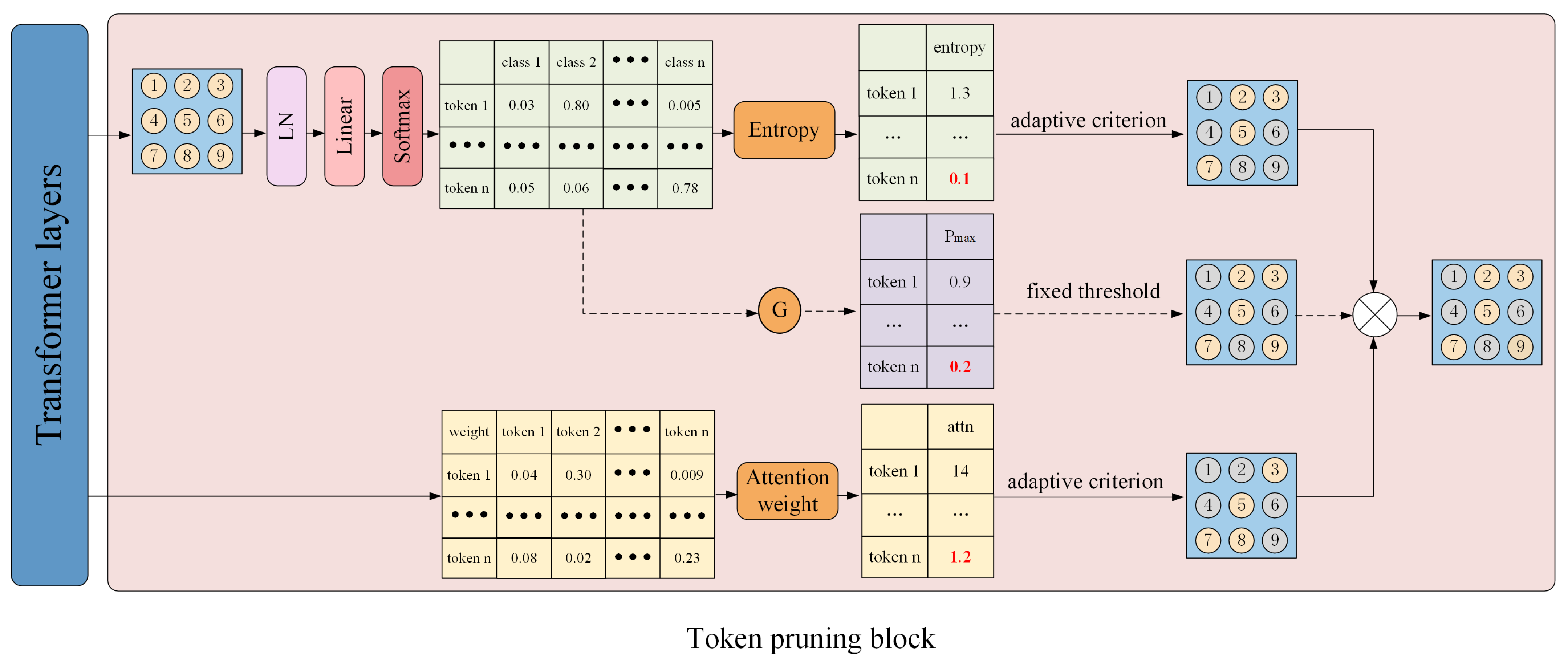
3.1. Architectural Configuration of MATP

In plain ViT [1] architectures, the input image $X\in {\mathbb{R}}^{H\times W\times 3}$ undergoes patch partitioning into non-overlapping ${\displaystyle \frac{HW}{P^2}}\times C$ regions, where $H,W$ denotes the original spatial resolution, P represents the patch size, and C denotes the dimension. Through linear projection, these patches are embedded into a sequence of visual tokens with certain dimensions, yielding an initial token sequence of length $N={\displaystyle \frac{HW}{P^2}}$ and shape ${\mathbb{R}}^{N\times C}$. To address the model’s inherent lack of spatial awareness, learnable positional encodings are incorporated to preserve position relations between tokens, resulting in the encoded input sequence for the transformer encoder. ViT [1] extracts image information through stacked encoder layers composed of multi-head self-attention modules and feed-forward networks, along with layer normalization [43] and residual connections [44]. The output of the stacked encoder layers is the feature x that ViT extracts from input image X. The length of x denotes n.

As shown in Figure 1, we divide a plain ViT backbone into M stages and we insert a token pruning block with an auxiliary head to calculate the mask at the end of each stage. Finally, we reconstruct the pruned tokens and keep these tokens after the final encoder layer to form a complete feature map for the decoder prediction.

3.2. Lightweight Auxiliary Heads

Most existing token pruning methods derive pruning scores either through auxiliary prediction heads [6,45] or several convolution layers [14,16,23]. Early work [6] used decoders as auxiliary heads, like the attention-to-mask module [46], which brought much extra computational cost. To decrease the extra computational cost, we simplify the auxiliary head. It consists of a LayerNorm [43], denoted as LN; a single linear layer, denoted as Linear; and a softmax to obtain the prediction, denoted as $\overrightarrow{pred}$, according to the input feature, denoted as $\overrightarrow{x}$ as follows:

$$\overrightarrow{pred}=\mathrm{Softmax}\left(\mathrm{Linear}\left(\mathrm{LN}\left(\overrightarrow{x}\right)\right)\right)$$

(1)

Lightweight auxiliary heads can significantly decrease the computational cost of a model with only a little degradation in accuracy. This means we do not need so much computation to obtain a very precise prediction if we just want a score to represent the learning progression of each token accurately. We block the gradient propagation of auxiliary heads. Since the predictions of the auxiliary heads are not extremely accurate, we do not want the prediction of the final decoder to be affected by the prediction of the auxiliary heads. Thus, we isolate the lightweight auxiliary heads from the backbone, which is training-efficient too. As a result, the backbone is only supervised by the loss of the decoder, with less accuracy degradation.

3.3. Multi-Faceted Token Pruning

One important reason for the accuracy degradation caused by token pruning is the loss of information contained in the pruned tokens. This information helps models to classify each pixel for semantic segmentation. Thus, we divided the information of tokens into two categories, enabling them to recognize themselves and to recognize other tokens. To decrease the loss of information, we need to evaluate the information of the tokens before pruning. We employ learning progression and relations between tokens as two metrics to measure the two categories of information the token contains and decide whether to prune the token or not. If a token has been learned better, pruning it causes less information loss. But if a token has closer relations with another token, pruning it causes more information loss. As illustrated in Figure 2, we conduct token pruning from three perspectives during training and two perspectives during inference, to select well-learned tokens without close relations to others to reduce computational cost with less accuracy degradation.

To quantitatively assess the learning progression of visual tokens, we employ information entropy [22] as a pruning score. Information entropy quantifies the uncertainty of an object’s possible states, while simultaneously characterizing the information it contains [22]. Theoretically, decreasing entropy values reflects increasing classification confidence. When the classification confidence of the token is high, the token is usually learned well. In other words, minimal entropy often indicates that the token is well-learned. Entropy takes into account the probabilities of all classes. In contrast to relying solely on the maximum probability [6], it has the potential to more effectively assess the learning progression of tokens, particularly in situations where the prediction accuracy is suboptimal. When two tokens have the same maximum possibility, their entropy values are usually different. The token with lower entropy is regarded as being classified in less classes and contains less information. The entropy in this paper is calculated as follows:

$$\mathrm{H}\left(x_i\right)=-\sum _{j=1}^m{p}_{i,j}\ln \left(p_{i,j}\right)$$

(2)

where $p_{i,j}$ denotes the prediction possibility of the i-th token in $pred$ belonging to the j-th class, $x_i$ denotes the i-th token in the input feature x, and m denotes the class number.

We choose attention weight to represent relations between tokens as another pruning score. Based on the mathematical significance of the attention weights, we find that the weight value in the attention mechanism, when it is summed over the spatial dimensions, reflects the relations between each token and other tokens. Originally, when the query (Q) and the key (K) are equal to the input feature x, $Q{K}^T$ represents the similarity of each token in the feature. In vision transformers [1,2], Q and K are generated through learnable linear layers whose parameters are optimized via backpropagation under loss supervision. Consequently, the attention matrix $Q{K}^T$ inherently encodes relations between tokens that represent how strongly each token influences others toward making accurate predictions. As a result, we export the weights from the attention layer and just conduct summation to obtain the attention weight score. Thus, we reduce the extra calculation for obtaining the second score. Obviously, the more closely a token is related to other tokens, the more significant its impact on the learning process of other tokens. Therefore, we choose to retain a subset of the tokens with the highest attention weights to mitigate the accuracy degradation caused by pruning. Attention weight is calculated as follows:

$$Attn=\sum _{i=1}^n\mathrm{Softmax}\left({\displaystyle \frac{Q{K}^T}{\sqrt{d_k}}}\right),Q,K=\mathrm{Linear}\left(x\right)$$

(3)

where $Attn$ denotes the attention weight of a sequence. n denotes the length of the sequence. $d_k$ is the scale factor as a fixed value. x denotes the input features.

Many tokens are pruned in the early stages of training, when the overall learning quality is poor, due to our adaptive criteria. This does not align with our principle of pruning well-learned tokens and is not conducive to obtaining global information to promote learning. Therefore, we set a train-time retention gate. The gate retains tokens that learned poorly in the early stages of training.

When these tokens learned well in the late stages of training, the retained tokens are pruned. When the maximum probability, denoted as $p_{max}$, of the i-th token, as an easily obtained score from the existing auxiliary head, is less than the gate threshold, denoted as $\varphi$, the gate retains the token as $p_{max}^i<\varphi$ to decrease premature information loss. This helps accelerate parameter adjustment during training and improves training effectiveness. The train-time retention gate is removed during inference. The gate generates the mask, denoted as $\overrightarrow{mas{k}_G}$, as follows:

$$\begin{array}{cc}\hfill & \overrightarrow{mas{k}_G}=\left[M_{G_1},M_{G_2},\dots ,M_{G_n}\right],\hfill \\ \hfill & M_{G_i}=\left\{\begin{array}{cc}1\hfill & \mathrm{if}{p}_{max}^i>\varphi ,\hfill \\ 0\hfill & \mathrm{otherwise}.\hfill \end{array}\right.\hfill \end{array}$$

(4)

It is crucial to set an appropriate train-time retention gate, as it should neither be too small nor too large. On the one hand, if the threshold is too small, none of the tokens are stopped by the train-time retention gate. Consequently, the gate becomes ineffective in accelerating training. On the other hand, the parameters may not sufficiently contribute to the learning of tokens if pruned within just a few layers, since the token is typically retained until the final layer during training. As a result, when tokens are pruned during inference, the final prediction accuracy may be compromised significantly.

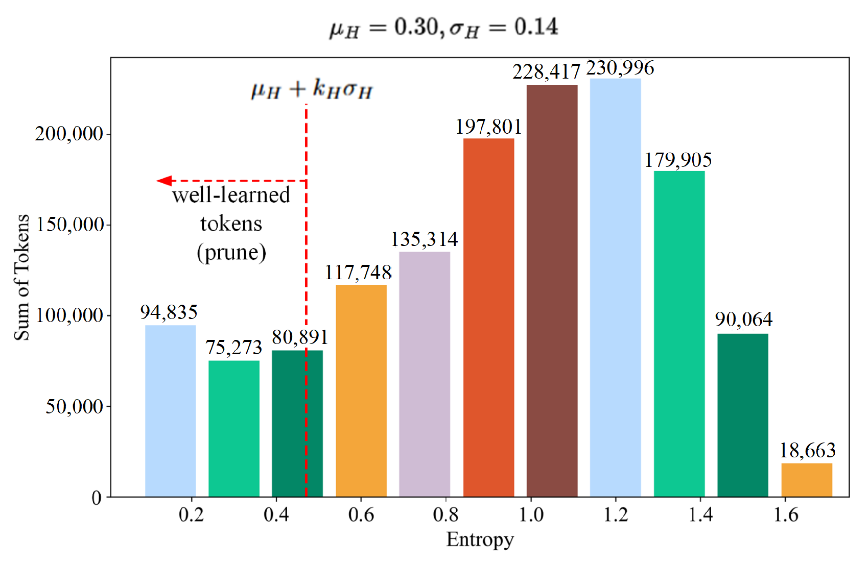
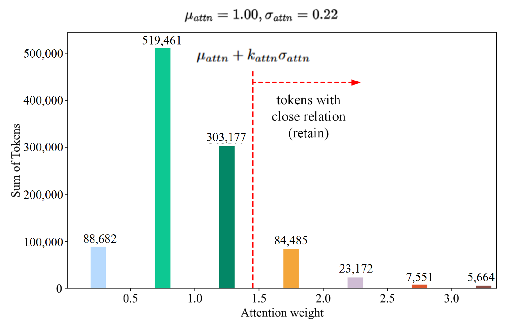
3.4. Adaptive Token Pruning Criteria

Another core part of token pruning is the pruning criteria. Traditional token pruning methods using a fixed pruning ratio or threshold cannot dynamically adjust the criteria according to the exact learning situation, which usually is not suitable for RS imagery. Therefore, we employ adaptive pruning criteria, which automatically adjust based on specific input features, ensuring the criteria remain relevant across diverse input features. Each score has its own pruning criteria.

We deem that in a normally captured natural image, the difficulty of learning for all tokens approximately follows a normal distribution. As shown in Figure 3, we can observe that the frequency distribution of the entropy on the Potsdam test set [47] is generally close to a normal distribution. As a result, we think tokens with entropy less than the sum of the mean and variance are considered to be relatively well-learned compared to the entire image. The pruning criterion to generate the mask is as follows:

$$\mathrm{H}\left(x_i\right)<{\mu }_H+k_H{\sigma }_H$$

(5)

$$\begin{array}{cc}\hfill & \overrightarrow{mas{k}_H}=\left[M_{H_1},M_{H_2},\dots ,M_{H_n}\right],\hfill \\ \hfill & M_{H_i}=\left\{\begin{array}{cc}1\hfill & \mathrm{if}\mathrm{H}\left(x_i\right)<{\mu }_H+k_H{\sigma }_H,\hfill \\ 0\hfill & \mathrm{otherwise}.\hfill \end{array}\right.\hfill \end{array}$$

(6)

where $H\left(x_i\right)$ denotes the entropy value of the i-th token; ${\mu }_H$ denotes the mean of the entropy of the feature; $k_H$ denotes an adjustable coefficient based on the specific task requirements, with a default value of 1.2; and ${\sigma }_H$ denotes the variance of the entropy of the feature. According to the criterion, we generate the mask denoted as $\overrightarrow{mas{k}_H}$. As for the window self-attention mechanism, it demands the input feature to be resized to a rectangle shape, while token pruning changes the length of sequence and usually cannot be resized to a rectangle shape again. Thus, we keep the shape of the feature map between encoder layers, using zero to fill the mask, and just conduct token pruning in each window before calculating attention. To ensure parallel processing, we calculate the pruning ratio of all the windows according to the overall learning progression, like global attention. With the same pruning ratio, every window has the same shape and all the windows can be processed simultaneously.

We also believe that in a normally captured natural image, the relations between tokens follow a similar normal distribution. As shown in Figure 4, we can observe that the frequency distribution of the entropy on the Potsdam test set [47] is generally close to a normal distribution. Thus, we set the pruning criterion for relations between tokens as represented by the attention weight. We consider tokens with attention weights greater than the mean plus the standard deviation of all tokens’ attention weights as the tokens closely related to other tokens. These tokens should not be pruned due to the information they contain and their influence on other tokens. The criterion to generate the mask is as follows:

$$A_i<{\mu }_{attn}+k_{attn}{\sigma }_{attn}$$

(7)

$$\begin{array}{cc}\hfill & \overrightarrow{mas{k}_A}=\left[M_{A_1},M_{A_2},\dots ,M_{A_n}\right],\hfill \\ \hfill & M_{A_i}=\left\{\begin{array}{cc}1\hfill & \mathrm{if}{A}_i<{\mu }_{attn}+k_{attn}{\sigma }_{attn},\hfill \\ 0\hfill & \mathrm{otherwise}.\hfill \end{array}\right.\hfill \end{array}$$

(8)

where $A_i$ denotes the attention weights of the i-th token, ${\mu }_{attn}$ denotes the mean of the attention weights, and ${\sigma }_{attn}$ denotes the standard deviation of the attention weights. $k_{attn}$ denotes a hyper-parameter. According to the criterion, we obtain the mask denoted as $\overrightarrow{mas{k}_A}$.

We finally obtain a mask, denoted as final mask $\overrightarrow{mas{k}_f}$, based on the three masks mentioned above. The final mask decides which tokens to prune. We denote kept tokens as $\overrightarrow{token{s}_k}$ and pruned tokens as $\overrightarrow{token{s}_p}$. We index tokens denoted as x by $i\in \{a,b,\dots ,n\}$ for pruned tokens and $I\in \{A,B,\dots ,N\}$ for kept tokens. The process is as follows:

$$\overrightarrow{mas{k}_f}=\overrightarrow{mas{k}_H}\times \overrightarrow{mas{k}_A}\times \overrightarrow{mas{k}_G}$$

(9)

$$\begin{array}{c}\hfill \left\{\begin{array}{cc}\overrightarrow{token{s}_k}=[x_A^p,x_B^p,\dots ,x_N^p],\hfill & \mathrm{if}mas{k}_{f_I}=0\hfill \\ \overrightarrow{token{s}_p}=[x_a^p,x_b^p,\dots ,x_n^p],\hfill & \mathrm{if}mas{k}_{f_i}=1\hfill \end{array}\right.\end{array}$$

(10)

The final output of the encoder, denoted as $fp$, is affected by the final mask. To reconstruct tokens for a complete feature map, if the tokens are masked, we fill the output positions with the aligned tokens propagated from the layers where they are pruned. We index layers as $l\in \{1,2,\dots ,L\}$. The token propagated from the layer where it is pruned is denoted as $x_i^p$. This process can be modeled as follows:

$$\begin{array}{cc}\hfill & \overrightarrow{f{p}^l}=\left[x_1,x_2,\dots ,x_n\right],\hfill \\ \hfill & x_i=\left\{\begin{array}{cc}{x}_i^l\hfill & \mathrm{if}mas{k}_{f_i}=0,\hfill \\ x_i^p\hfill & \mathrm{otherwise}.\hfill \end{array}\right.\hfill \end{array}$$

(11)

4. Experiments

This section presents a comprehensive analysis of the experimental performance of MATP on three RS semantic segmentation datasets and compares it with other existing methods in the field. The experimental results demonstrate that our MATP method effectively achieves a significant reduction in computational cost while ensuring minimal loss of accuracy, surpassing the SOTA.

4.1. Segmentation Datasets

Our method is tested on three mainstream RS semantic segmentation datasets: Potsdam [47], LoveDA [48], and Five-Billion-Pixels [49].

The LoveDA dataset [48] contains 5987 high-resolution optical RS images (with a ground sampling distance of 0.3 m), each sized at 1024 × 1024 pixels, covering 7 land cover classes. The dataset includes 2522 training images, 1669 validation images, and 1796 test images. But according to the configuration file in mmsegmentation, we ignore the original test set and use the validation test set as the new test set.

The Potsdam dataset [47] consists of 38 high-resolution aerial RS images, each sized at 6000 × 6000 pixels, with a spatial resolution of 0.05 m. The dataset covers 6 major land cover classes: impervious surfaces, buildings, low vegetation, trees, cars, and background. It includes 3456 training images, 1008 validation images, and 1008 test images.

The Five-Billion-Pixels dataset [49] contains over 5 billion labeled pixels, composed of 150 high-resolution Gaofen-2 satellite images with a spatial resolution of 4 m. These images cover an area of over 50,000 square kilometers and include 24 land cover classes. The dataset includes 18,900 training images, 6300 validation images, and 6300 test images.

4.2. Experimental Setup

To demonstrate the generalization ability of the MATP method for semantic segmentation tasks, we conduct experiments on three datasets: LoveDA [48], Potsdam [47], and Five-Billion-Pixels [49]. In these experiments, we use SegViT [46] as the segmentation head, and the data processing and training protocols are also the same as those of DToP [6]. We train the model for 40k iterations on all three datasets, and the batch size is 4 during training and 1 during testing and validation. The cropped image patch size is 512 × 512. All experiments in this paper are completed on a Windows 10 platform, Intel Core i7-8700 CPU, using the PyTorch 2.3.1 framework and an NVIDIA GeForce RTX 2070 GPU. The specific configurations are shown in

Table 1. Training settings of semantic segmentation on the three datasets.

Training Config	MATP
Image size	512 × 512
Train and validation size	512 × 512
Patch size	16
Number of heads	12
Prune layers	3, 6, 8
Optimizer	AdamW
Learning rate	2 × 10−4
Weight decay	0.01
Batch size	4
Training iterations	40,000
Main loss	Cross-entropy loss
Auxiliary loss	Attention to mask loss

.

4.3. Experimental Results

Table 2. Comparison with existing mainstream token reduction methods. Red bold and blue bold denote the best and second-best performance in each column. An upward arrow indicates that a higher value for the metric is better, while a downward arrow indicates that a lower value is better.

Method	Decoder	Dataset	Publication	Params. (M)↓	mIoU (%)↑	FLOPs (G)↓
ViT-B [1]	SegViT [46]	Potsdam [47]	NIPS2022	93.83	79.20	108.27
+ToMe [41]	SegViT [46]	Potsdam [47]	ICLR2023	93.80	62.55 (−16.65%)	62.40 (−42.4%)
+DToP [6]	SegViT [46]	Potsdam [47]	IEEE ICCV2023	109.00	74.43 (−4.77%)	33.51 (−69.0%)
+ALGM [18]	SegViT [46]	Potsdam [47]	IEEE CVPR2024	93.83	74.88 (−4.32%)	30.49 (−71.8%)
+ours	SegViT [46]	Potsdam [47]	-	94.75	76.33 (−2.87%)	33.97 (−68.6%)
ViT-B [1]	SegViT [46]	LoveDA [48]	NIPS2022	93.83	52.75	108.28
+ToMe [41]	SegViT [46]	LoveDA [48]	ICLR2023	93.80	41.25 (−11.5%)	62.42 (−42.4%)
+DToP [6]	SegViT [46]	LoveDA [48]	IEEE ICCV2023	109.00	49.37 (−3.38%)	33.43 (−69.1%)
+ALGM [18]	SegViT [46]	LoveDA [48]	IEEE CVPR2024	93.83	49.20 (−3.55%)	34.23 (−68.4%)
+ours	SegViT [46]	LoveDA [48]	-	94.75	49.83 (−2.92%)	33.57 (−69.0%)
ViT-B [1]	SegViT [46]	FBP [49]	NIPS2022	93.83	60.74	108.44
+ToMe [41]	SegViT [46]	FBP [49]	ICLR2023	93.80	37.49 (−23.25%)	62.58 (−42.3%)
+DToP [6]	SegViT [46]	FBP [49]	IEEE ICCV2023	109.00	51.99 (−8.75%)	41.28 (−61.9%)
+ALGM [18]	SegViT [46]	FBP [49]	IEEE CVPR2024	93.83	52.56 (−8.18%)	30.77 (−71.6%)
+ours	SegViT [46]	FBP [49]	−	94.75	54.64 (−6.10%)	35.05 (−67.7%)

provides a detailed comparison of our method with other mainstream token reduction methods on the LoveDA validation set [48], Potsdam test set [47], and Five-Billion-Pixels test set [49]. As Table 2 shows, we achieve a better trade-off between computational cost and accuracy on all three datasets. Figure 5 may show the trade-off more obviously compared with an RS lightweight network. On the Potsdam test set [47], compared with ALGM [18], we achieve a 1.50% higher mIoU with similar FLOPs. On the LoveDA validation set [48], our method achieves an 0.46% mIoU improvement with just 0.14 G more FLOPs compared with DToP [6]. On the Five-Billion-Pixels [49] test set, we achieve the highest accuracy with comparable computational cost, exceeding ALGM [21] by 2.08%. According to

Table 3. Comparison with existing mainstream token reduction methods on Swin Transformer [2]. Red bold and blue bold denote the best and second-best performance in each column. An upward arrow indicates that a higher value for the metric is better, while a downward arrow indicates that a lower value is better.

Method	Decoder	Dataset	Publication	Params. (M)↓	mIoU (%)↑	FLOPs (G)↓ (Encoder)	FLOPs (G)↓ (Decoder)
Swin-T [2]	UPerNet [50]	Potsdam [47]	IEEE ICCV2021	59.83	80.03	25.61	210.36
+ELViT [21]	UPerNet [50]	Potsdam [47]	NIPS2022	52.80	67.08	17.39	210.36
+SparseViT [42]	UPerNet [50]	Potsdam [47]	IEEE CVPR2023	59.85	76.99	14.61	210.36
+ours	UPerNet [50]	Potsdam [47]	-	59.31	77.89	17.76	210.36
Swin-T [2]	UPerNet [50]	LoveDA [48]	IEEE ICCV2021	59.83	52.36	25.61	210.38
+ELViT [21]	UPerNet [50]	LoveDA [48]	NIPS2022	52.80	38.80	17.49	210.38
+SparseViT [42]	UPerNet [50]	LoveDA [48]	IEEE CVPR2023	59.85	48.36	14.63	210.38
+ours	UPerNet [50]	LoveDA [48]	-	59.31	49.31	16.96	210.38
Swin-T [2]	UPerNet [50]	FBP [49]	IEEE ICCV2021	59.83	60.48	25.62	210.51
+ELViT [21]	UPerNet [50]	FBP [49]	NIPS2022	52.80	31.50	17.49	210.51
+SparseViT [42]	UPerNet [50]	FBP [49]	IEEE CVPR2023	59.85	50.27	14.63	210.51
+ours	UPerNet [50]	FBP [49]	-	59.31	52.05	17.25	210.51

, our approach also surpasses existing token reduction methods on Swin Transformer [2], with 1.80%, 0.95%, and 1.78% mIoU improvements, respectively, on the Potsdam test set [47], LoveDA validation set [48], and Five-Billion-Pixels set [49]. Comparing the accuracy drop on the Potsdam [47] and LoveDA [48] datasets with the FBP [49] dataset, the accuracy drop on the FBP [49] dataset is relatively large. We think its class number is the reason. Its 24 classes is more than the 6 classes of the Potsdam [47] dataset and the 8 classes of the LoveDA [48] dataset. As a result, the loss of detail information may cause mistakes for similar classes.

Table 4. Comparison of mainstream lightweight methods for RS. Red bold and blue bold denote the best and second-best performance in each column. An upward arrow indicates that a higher value for the metric is better, while a downward arrow indicates that a lower value is better.

Method	Decoder	Dataset	Publication	Params. (M)↓	mIoU (%)↑	FLOPs (G)↓
ResNet50 [44]	FactSeg [37]	Potsdam [47]	TGRS2021	33.46	76.61	68.08
ResNet18 [44]	UnetFormer [4]	Potsdam [47]	ISPRS2022	12.31	60.82	13.01
DecoupleNet-D2 [12]	UnetFormer [4]	Potsdam [47]	TGRS2024	7.33	65.21	8.11
ResNet50 [44]	LoveNAS [38]	Potsdam [47]	ISPRS2024	30.51	75.93	44.40
ViT-B [1] +ours	SegViT [46]	Potsdam [47]	-	94.75	76.33	33.97
ResNet50 [44]	FactSeg [37]	LoveDA [48]	TGRS2021	33.46	48.07	68.09
ResNet18 [44]	UnetFormer [4]	LoveDA [48]	ISPRS2022	12.31	37.91	13.02
DecoupleNet-D2 [12]	UnetFormer [4]	LoveDA [48]	TGRS2024	7.33	43.88	8.12
ResNet50 [44]	LoveNAS [38]	LoveDA [48]	ISPRS2024	30.51	48.86	44.40
ViT-B [1] +ours	SegViT [46]	LoveDA [48]	-	94.75	49.83	33.57
ResNet50 [44]	FactSeg [37]	FBP [49]	TGRS2021	33.46	54.78	68.14
ResNet18 [44]	UnetFormer [4]	FBP [49]	ISPRS2022	12.31	32.94	13.05
DecoupleNet-D2 [12]	UnetFormer [4]	FBP [49]	TGRS2024	7.33	26.00	8.15
ResNet50 [44]	LoveNAS [38]	FBP [49]	ISPRS2024	30.51	32.75	44.45
ViT-B [1] +ours	SegViT [46]	FBP [49]	-	94.75	54.64	35.05

provides a detailed comparison between our method and other mainstream lightweight methods in RS on the same three datasets. As Table 4 shows, we achieve similar or even higher accuracy to FactSeg [37] with nearly half of the computational cost. And we achieve higher accuracy and lower computational cost than LoveNAS [38] on the Potsdam test set [47], LoveDA validation set [48], and Five-Billion-Pixels set [49], with 0.40%, 0.97%, 21.89% accuracy increases and 10.43 G, 10.83 G, 9.00 G computation decreases relatively. Figure 5 shows the comparison of accuracy and computational cost trade-off more clearly.

To evaluate the robustness of MATP, we introduced random noise to the input images during inference without retraining.

Table 5. Performance of MATP and baseline with random noise. Baseline uses ViT [1] as backbone and SegViT [46] as decoder. An upward arrow indicates that a higher value for the metric is better.

Method	mIoU (%)↑ with 0 Pixels Noise	mIoU (%)↑ with 100 Pixels Noise	mIoU (%)↑ with 1000 Pixels Noise
Baseline	79.20	79.17	78.04
+MATP	76.33	76.25	74.66

shows that noise affects the pruning decisions, as error information of the noise disrupts MATP’s token selection. Nevertheless, MATP’s performance remains relatively stable under moderate noise, demonstrating some inherent noise resistance.

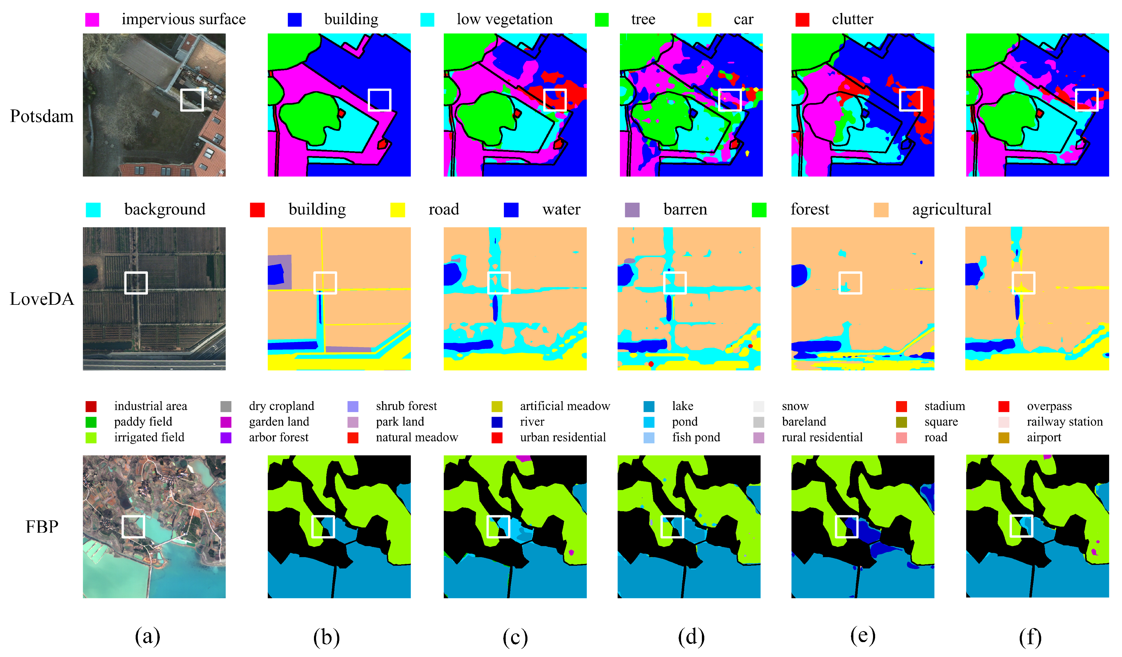
4.4. Visualization Results

The visualization results of the masks of pruned tokens after three, six, and eight layers on the Potsdam test set are presented in Figure 6. The earlier-token-pruning approach [6] is less sensitive to the learning progression of tokens, which often leads to erroneously detecting well-learned tokens. These masks demonstrate the superiority of our approach in adaptively selecting tokens to prune according to the learning progression of each token. Remaining sensitive to the learning progression of each token, our approach detects well-learned tokens to prune, which leads to less information loss and less accuracy degradation. The visual prediction results of different methods on the Potsdam test set [47], LoveDA validation set [48], and Five-Billion-Pixels test set [49] are presented in Figure 7. As Figure 7 shows, on the Potsdam test set [47] our method identifies the building on the edge of building and impervious surface in the box while others classify the building here as clutter. On the LoveDA validation set [48], our method recognizes the roads between agricultural regions while the others just regard them as background. On the Five-Billion-Pixels test set, our method distinguishes pond, lake, and river near the bank correctly and classifies the region in the box as lake, while the others make mistakes. These demonstrate the capability of our approach in recognizing objects around edges, as a result of the multi-faceted adaptive token pruning used to decrease the information loss.

4.5. Ablation Studies

This section outlines the ablation experiments that are conducted to dissect the contributions of the key parts in MATP and to evaluate the influence of the coefficients on the Potsdam [47], LoveDA [48], and Five-Billion-Pixels [49] datasets for semantic segmentation.

(1) Effectiveness analysis of each part of MATP: In

Table 6. The effects of the main parts of our approach. These experiments are conducted on the Potsdam [47] test set. The baseline is ViT-B [1] + SegViT [46]. The pruning positions in this table are layers 3, 6, and 8. Red bold and blue bold denote the best and second-best performance in each column. An upward arrow indicates that a higher value for the metric is better, while a downward arrow indicates that a lower value is better. “✓” means model with this module and “×” means model with this module.

Random Token Pruning	Adaptive Entropy-Based Token Pruning	Lightweight Auxiliary Heads	Relation-Based Tokens Retained	Gradient Stop	mIoU (%)↑	FLOPs (G)↓
×	×	×	×	×	79.35	108.27
✓	×	×	×	×	75.60	38.01
×	✓	×	×	×	75.21	33.05
×	✓	✓	×	×	75.91	32.88
×	✓	✓	✓	×	76.25	33.93
×	✓	✓	✓	✓	76.33	33.97

, “random token pruning” means pruning tokens randomly without any scores or criteria. “Adaptive entropy-based token pruning” refers to the use of an adaptive pruning criteria and entropy scores for discrimination. “Lightweight auxiliary heads” denotes the use of lightweight auxiliary heads to obtain scores. “Relation-based tokens retained” indicates the retention of tokens based on attention weights. “Gradient stop” refers to gradient blocking, which prevents the gradients from the auxiliary head from affecting the encoder parameters. And we can observe that compared to the first row, adaptive pruning can significantly reduce computational cost with minimal loss in accuracy. The lightweight auxiliary head results in a 4.10% decrease in mIoU and a reduction of 75.20 G in computational cost. Comparing the third row with the second, we find that after using the lightweight auxiliary head, the accuracy improves while the computation decreases, which seems counterintuitive. In fact, this is because computational cost of the auxiliary heads is reduced and the overall number of pruned tokens become fewer, leading to improved accuracy and less computation drop. Comparing the fourth row with the third, retaining some tokens based on attention weights, with an increase of 1.00 G in computational cost, the accuracy is improved by 0.34%, indicating that it indeed retains some tokens that are relatively important for subsequent learning. Comparing the sixth row with the fifth, blocking the gradients of the auxiliary head to prevent it from affecting the encoder parameters effectively improves accuracy.

(2) Comparative analysis of different pruning methods: In

Table 7. Comparison of existing mainstream token pruning scores and criteria and ours on Potsdam [47] test set. The pruning locations of this experiment are layers 6 and 8, which is consistent with DToP [6]. The decoder is SegViT [46]. Bold denotes the best performance in each column. An upward arrow indicates that a higher value for the metric is better, while a downward arrow indicates that a lower value is better.

Method	mIoU (%)↑	FLOPs (G)↓
ViT-B [1]	79.35	108.27
Random	78.54	70.80
Pruning topk ($k=500$)	78.51	64.78
Fix threshold ($r>0.9$)	77.82	65.63
Adaptive entropy-based	78.64	58.65

, “random” indicates random pruning, “topk” refers to pruning the k tokens with the most concentrated prediction probabilities, “fix threshold” denotes pruning with a fixed threshold and the maximum prediction possibility score, and “adaptive entropy” represents the use of our adaptive pruning criterion and entropy score. As Table 7 shows, our adaptive entropy pruning criteria achieve the highest accuracy and the lowest computational cost among various pruning criteria commonly used in existing works [6,14,16,45]. The accuracy exceeds random token pruning by 0.10%, and the computational cost is 6.13 G lower than topk token pruning. This result demonstrates the advancement of the adaptive entropy pruning criterion.

(3) Effectiveness analysis of different gate thresholds: As for the train-time retention gate, we conduct experiments when the value of the gate threshold $\varphi$ is 0, 0.2, 0.4, 0.6, 0.8, and 1.0. Since the threshold is only used during training, the computational cost during inference remains almost unchanged. As illustrated in

Table 8. Comparison of different train-time retention gate on Potsdam [47] test set. Bold denotes the best performance in each column. Bold denotes the best performance in each column. An upward arrow indicates that a higher value for the metric is better.

$\mathit{\varphi }$	mIoU (%)↑
0	75.54
0.2	76.11
0.4	75.47
0.6	75.59
0.8	74.09
1.0	18.50

, it is obvious that retaining less tokens does not improve training and retaining more tokens makes parameters not fit to pruned tokens during inference. Especially, when $\varphi$ is 1.0, it does not prune any tokens. Predictions for tokens that do not propagate through the entire encoder are not supervised by any loss. Consequently, the predictions are frequently inaccurate, resulting in low accuracy.

(4) Effectiveness analysis of different pruning locations: We conduct a pruning location analysis experiment following DToP [6]; the results are shown in

Table 9. Comparison of different pruning positions on Potsdam [47] test set. This experiment is consistent with DToP [6]. Bold denotes the best performance in each column. An upward arrow indicates that a higher value for the metric is better, while a downward arrow indicates that a lower value is better.

lpruning	mIoU (%)↑	FLOPs (G)↓
6	78.52	63.62
8	79.02	77.89
6, 8	78.51	59.24
3, 6, 8	76.33	33.97

. Comparing the first line with the second line and the third line with the fourth line, we can find that the change in the location of the first pruning usually leads to an obvious drop in mIoU and FLOPs. Instead, comparing the first line with the third line, when the location of the first pruning is unchanged, the second pruning leads to a 0.01% and 4.38 G drop in mIoU and FLOPs, respectively. We find that accuracy and computational cost are closely related to the first pruning and its location, and distantly related to the second pruning. We choose to prune after the third, sixth and eighth layers, with the least computational cost as default.

(5) Effectiveness analysis of different values of two coefficients : We also conduct experiments to explore the effectiveness of two coefficients in the pruning criteria. As shown in

Table 10. Comparison of different coefficient values of $k_H$ and $k_{attn}$ in adaptive pruning criteria on Potsdam [47] test set. Bold denotes the best performance in each column. Bold denotes the best performance in each column. An upward arrow indicates that a higher value for the metric is better, while a downward arrow indicates that a lower value is better.

${\mathit{k}}_{\mathit{H}}$	${\mathit{k}}_{\mathbf{attn}}$	mIoU (%)↑	FLOPs (G)↓
0.3	2.0	77.24	44.29
0.6	2.0	77.05	39.99
0.9	2.0	76.69	36.39
1.2	0.5	77.08	44.29
1.2	1.0	76.47	36.31
1.2	1.5	76.37	34.67
1.2	2.0	76.33	33.97

, $k_H$ is positively correlated with the number of pruned tokens. And according to our observation, 1.2 is a proper value for the maximum compression ratio, because it prunes more than 1000 tokens out of 1024 tokens. And $k_{attn}$ is negatively correlated with the number of pruned tokens. The experimental analysis demonstrates that $k_{attn}=2.0$ achieves an optimal balance between computational cost and model accuracy, exhibiting a computational decrease of 0.70 GFLOPs, with only a marginal 0.04% accuracy reduction compared to the $k_{attn}=1.5$ configuration. This also reflects the fact that some tokens with close relations to others sometimes have similar information due to these relations being mutual. So we choose 1.2 for $k_H$ and 2 for $k_{attn}$ as default.

5. Discussion

According to the experiments, MATP reduces the computation cost of these models with acceptable accuracy degradation. On the one hand, MATP employs entropy to represent the learning progression and attention weights to represent the relation between tokens. On the other hand, it prunes tokens satisfying adaptive criteria that are adjusted automatically based on given specific input features. Thereby, MATP facilitates the utilization of vision transformers [1,2] in resource-constrained environments. It provides a new angle to gain lightweight vision transformers [1,2] for RS interpretation tasks. The experimental results on three widely used RS semantic segmentation datasets substantiate that MATP achieves a better trade-off than the SOTA on RS image segmentation. In the future, because the MATP framework provides a pruning method for the transformer encoder, it will be applied to other lightweight architectures to decrease the computation cost further. MATP will also be extended to other related tasks, such as change detection and object detection.

6. Conclusions

In this article, we propose MATP, a novel multi-faceted adaptive token pruning method for RS image segmentation, which fits vision transformers [1,2]. This stands in contrast to early token reduction works [6,14,15,16,17,18,21,23,41,42,45], which often used a fixed pruning ratio from only one perspective. To reduce the token redundancy of vision transformers [1,2] with less information loss, MATP prunes tokens adaptively from multiple perspectives. Our experiments demonstrate that entropy is appropriate to measure the learning progress of tokens and the attention weight can represent the relations between tokens. Our token pruning method decreases the information loss with a high compression rate and it provides a compression approach for most transformer-based models in remote sensing. Thus, the method can be applied to models in computational resource-constrained environment, helping models to be employed while maintaining its accuracy. However, the method can be affected by noise. The error information from noise will lead to erroneous token pruning. In addition, as the number of classes increases, a high pruning rate will cause a greater accuracy drop because the detail information is more important. While these limitations currently restrict wider applications of our method, we plan to investigate these challenges in future studies.

References

1. Dosovitskiy, A.; Beyer, L.; Kolesnikov, A.; Weissenborn, D.; Zhai, X.; Unterthiner, T.; Dehghani, M.; Minderer, M.; Heigold, G.; Gelly, S.; et al. An Image is Worth 16x16 Words: Transformers for Image Recognition at Scale. In Proceedings of the International Conference on Learning Representations, Vienna, Austria, 4 May 2021. [Google Scholar]
2. Liu, Z.; Lin, Y.; Cao, Y.; Hu, H.; Wei, Y.; Zhang, Z.; Lin, S.; Guo, B. Swin transformer: Hierarchical vision transformer using shifted windows. In Proceedings of the IEEE/CVF International Conference on Computer Vision, Montreal, QC, Canada, 11–17 October 2021; pp. 10012–10022. [Google Scholar]
3. Zhang, C.; Su, J.; Ju, Y.; Lam, K.M.; Wang, Q. Efficient inductive vision transformer for oriented object detection in remote sensing imagery. IEEE Trans. Geosci. Remote Sens. 2023, 61, 5616320. [Google Scholar] [CrossRef]
4. Wang, L.; Li, R.; Zhang, C.; Fang, S.; Duan, C.; Meng, X.; Atkinson, P.M. UNetFormer: A UNet-like transformer for efficient semantic segmentation of remote sensing urban scene imagery. ISPRS J. Photogramm. Remote Sens. 2022, 190, 196–214. [Google Scholar] [CrossRef]
5. Khan, S.; Naseer, M.; Hayat, M.; Zamir, S.W.; Khan, F.S.; Shah, M. Transformers in vision: A survey. ACM Comput. Surv. 2022, 54, 1–41. [Google Scholar] [CrossRef]
6. Tang, Q.; Zhang, B.; Liu, J.; Liu, F.; Liu, Y. Dynamic token pruning in plain vision transformers for semantic segmentation. In Proceedings of the IEEE/CVF International Conference on Computer Vision, Paris, France, 1–6 October 2023; pp. 777–786. [Google Scholar]
7. Lei, T.; Geng, X.; Ning, H.; Lv, Z.; Gong, M.; Jin, Y.; Nandi, A.K. Ultralightweight spatial—Spectral feature cooperation network for change detection in remote sensing images. IEEE Trans. Geosci. Remote Sens. 2023, 61, 4402114. [Google Scholar] [CrossRef]
8. Zhang, C.; Jiang, W.; Zhang, Y.; Wang, W.; Zhao, Q.; Wang, C. Transformer and CNN Hybrid Deep Neural Network for Semantic Segmentation of Very-High-Resolution Remote Sensing Imagery. IEEE Trans. Geosci. Remote Sens. 2022, 60, 4408820. [Google Scholar] [CrossRef]
9. Wu, H.; Huang, P.; Zhang, M.; Tang, W.; Yu, X. CMTFNet: CNN and multiscale transformer fusion network for remote-sensing image semantic segmentation. IEEE Trans. Geosci. Remote Sens. 2023, 61, 2004612. [Google Scholar] [CrossRef]
10. Li, R.; Zheng, S.; Zhang, C.; Duan, C.; Wang, L.; Atkinson, P.M. ABCNet: Attentive bilateral contextual network for efficient semantic segmentation of Fine-Resolution remotely sensed imagery. ISPRS J. Photogramm. Remote Sens. 2021, 181, 84–98. [Google Scholar] [CrossRef]
11. Chen, H.; Qi, Z.; Shi, Z. Remote sensing image change detection with transformers. IEEE Trans. Geosci. Remote Sens. 2021, 60, 5900318. [Google Scholar] [CrossRef]
12. Lu, W.; Chen, S.B.; Shu, Q.L.; Tang, J.; Luo, B. DecoupleNet: A Lightweight Backbone Network With Efficient Feature Decoupling for Remote Sensing Visual Tasks. IEEE Trans. Geosci. Remote Sens. 2024, 62, 5935411. [Google Scholar] [CrossRef]
13. Lu, W.; Chen, S.B.; Ding, C.H.; Tang, J.; Luo, B. LWGANet: A Lightweight Group Attention Backbone for Remote Sensing Visual Tasks. arXiv 2025, arXiv:2501.10040. [Google Scholar]
14. Rao, Y.; Zhao, W.; Liu, B.; Lu, J.; Zhou, J.; Hsieh, C.J. DynamicViT: Efficient vision transformers with dynamic token sparsification. Adv. Neural Inf. Process. Syst. 2021, 34, 13937–13949. [Google Scholar]
15. Yin, H.; Vahdat, A.; Alvarez, J.M.; Mallya, A.; Kautz, J.; Molchanov, P. A-ViT: Adaptive tokens for efficient vision transformer. In Proceedings of the IEEE/CVF Conference on Computer Vision and Pattern Recognition, New Orleans, LA, USA, 18–24 June 2022; pp. 10809–10818. [Google Scholar]
16. Liang, Y.; Ge, C.; Tong, Z.; Song, Y.; Wang, J.; Xie, P. EViT: Expediting Vision Transformers via Token Reorganizations. In Proceedings of the International Conference on Learning Representations, Online, 25–29 April 2022. [Google Scholar]
17. Lu, C.; de Geus, D.; Dubbelman, G. Content-aware token sharing for efficient semantic segmentation with vision transformers. In Proceedings of the IEEE/CVF Conference on Computer Vision and Pattern Recognition, Vancouver, BC, Canada, 17–24 June 2023; pp. 23631–23640. [Google Scholar]
18. Norouzi, N.; Orlova, S.; De Geus, D.; Dubbelman, G. ALGM: Adaptive Local-then-Global Token Merging for Efficient Semantic Segmentation with Plain Vision Transformers. In Proceedings of the IEEE/CVF Conference on Computer Vision and Pattern Recognition, Seattle, WA, USA, 16–22 June 2024; pp. 15773–15782. [Google Scholar]
19. He, X.; Zhou, Y.; Zhao, J.; Zhang, D.; Yao, R.; Xue, Y. Swin Transformer Embedding UNet for Remote Sensing Image Semantic Segmentation. IEEE Trans. Geosci. Remote Sens. 2022, 60, 4408715. [Google Scholar] [CrossRef]
20. Kong, Z.; Dong, P.; Ma, X.; Meng, X.; Niu, W.; Sun, M.; Shen, X.; Yuan, G.; Ren, B.; Tang, H.; et al. SpViT: Enabling faster vision transformers via latency-aware soft token pruning. In Proceedings of the European Conference on Computer Vision, Tel Aviv, Israel, 23–27 October 2022; pp. 620–640. [Google Scholar]
21. Liang, W.; Yuan, Y.; Ding, H.; Luo, X.; Lin, W.; Jia, D.; Zhang, Z.; Zhang, C.; Hu, H. Expediting large-scale vision transformer for dense prediction without fine-tuning. Adv. Neural Inf. Process. Syst. 2022, 35, 35462–35477. [Google Scholar]
22. Shannon, C.E. A mathematical theory of communication. Bell Syst. Tech. J. 1948, 27, 379–423. [Google Scholar] [CrossRef]
23. Liu, Y.; Zhou, Q.; Wang, J.; Wang, Z.; Wang, F.; Wang, J.; Zhang, W. Dynamic token-pass transformers for semantic segmentation. In Proceedings of the IEEE/CVF Winter Conference on Applications of Computer Vision, Waikoloa, HI, USA, 3–8 January 2024; pp. 1827–1836. [Google Scholar]
24. Sandler, M.; Howard, A.; Zhu, M.; Zhmoginov, A.; Chen, L.C. MobileNetV2: Inverted residuals and linear bottlenecks. In Proceedings of the IEEE Conference on Computer Vision and Pattern Recognition, Salt Lake City, UT, USA, 18–23 June 2018; pp. 4510–4520. [Google Scholar]
25. Ma, N.; Zhang, X.; Zheng, H.T.; Sun, J. ShuffleNet v2: Practical guidelines for efficient cnn architecture design. In Proceedings of the European Conference on Computer Vision, Munich, Germany, 8–14 September 2018; pp. 116–131. [Google Scholar]
26. Zhang, X.; Zhou, X.; Lin, M.; Sun, J. ShuffleNet: An extremely efficient convolutional neural network for mobile devices. In Proceedings of the IEEE Conference on Computer Vision and Pattern Recognition, Salt Lake City, UT, USA, 18–23 June 2018; pp. 6848–6856. [Google Scholar]
27. Tan, M.; Chen, B.; Pang, R.; Vasudevan, V.; Sandler, M.; Howard, A.; Le, Q.V. Mnasnet: Platform-aware neural architecture search for mobile. In Proceedings of the IEEE/CVF Conference on Computer Vision and Pattern Recognition, Long Beach, CA, USA, 15–20 June 2019; pp. 2820–2828. [Google Scholar]
28. Li, Y.; Yuan, G.; Wen, Y.; Hu, J.; Evangelidis, G.; Tulyakov, S.; Wang, Y.; Ren, J. EfficientFormer: Vision transformers at MobileNet speed. Adv. Neural Inf. Process. Syst. 2022, 35, 12934–12949. [Google Scholar]
29. Li, Y.; Hu, J.; Wen, Y.; Evangelidis, G.; Salahi, K.; Wang, Y.; Tulyakov, S.; Ren, J. Rethinking vision transformers for MobileNet size and speed. In Proceedings of the IEEE/CVF International Conference on Computer Vision, Paris, France, 1–6 October 2023; pp. 16889–16900. [Google Scholar]
30. Ding, X.; Zhang, X.; Ma, N.; Han, J.; Ding, G.; Sun, J. RepVGG: Making VGG-style convnets great again. In Proceedings of the IEEE/CVF Conference on Computer Vision and Pattern Recognition, Nashville, TN, USA, 20–25 June 2021; pp. 13733–13742. [Google Scholar]
31. Yuan, L.; Chen, Y.; Wang, T.; Yu, W.; Shi, Y.; Jiang, Z.H.; Tay, F.E.; Feng, J.; Yan, S. Tokens-to-token ViT: Training vision transformers from scratch on ImageNet. In Proceedings of the IEEE/CVF International Conference on Computer Vision, Montreal, QC, Canada, 11–17 October 2021; pp. 558–567. [Google Scholar]
32. Carion, N.; Massa, F.; Synnaeve, G.; Usunier, N.; Kirillov, A.; Zagoruyko, S. End-to-end object detection with transformers. In Proceedings of the European Conference on Computer Vision, Glasgow, UK, 23–28 August 2020; pp. 213–229. [Google Scholar]
33. Zhu, X.; Su, W.; Lu, L.; Li, B.; Wang, X.; Dai, J. DETR: Deformable Transformers for End-to-End Object Detection. In Proceedings of the International Conference on Learning Representations, Vienna, Austria, 4 May 2021. [Google Scholar]
34. Cheng, B.; Misra, I.; Schwing, A.G.; Kirillov, A.; Girdhar, R. Masked-attention mask transformer for universal image segmentation. In Proceedings of the IEEE/CVF Conference on Computer Vision and Pattern Recognition, New Orleans, LA, USA, 18–24 June 2022; pp. 1290–1299. [Google Scholar]
35. Cheng, B.; Schwing, A.; Kirillov, A. Per-pixel classification is not all you need for semantic segmentation. Adv. Neural Inf. Process. Syst. 2021, 34, 17864–17875. [Google Scholar]
36. Dong, X.; Bao, J.; Chen, D.; Zhang, W.; Yu, N.; Yuan, L.; Chen, D.; Guo, B. CSWin transformer: A general vision transformer backbone with cross-shaped windows. In Proceedings of the IEEE/CVF Conference on Computer Vision and Pattern Recognition, New Orleans, LA, USA, 18–24 June 2022; pp. 12124–12134. [Google Scholar]
37. Ma, A.; Wang, J.; Zhong, Y.; Zheng, Z. FactSeg: Foreground activation-driven small object semantic segmentation in large-scale remote sensing imagery. IEEE Trans. Geosci. Remote Sens. 2021, 60, 5606216. [Google Scholar] [CrossRef]
38. Wang, J.; Zhong, Y.; Ma, A.; Zheng, Z.; Wan, Y.; Zhang, L. LoveNAS: Towards multi-scene land-cover mapping via hierarchical searching adaptive network. ISPRS J. Photogramm. Remote Sens. 2024, 209, 265–278. [Google Scholar] [CrossRef]
39. Chen, K.; Zou, Z.; Shi, Z. Building Extraction from Remote Sensing Images with Sparse Token Transformers. Remote Sens. 2021, 13, 4441. [Google Scholar] [CrossRef]
40. Chen, K.; Liu, C.; Chen, B.; Li, W.; Zou, Z.; Shi, Z. Dynamicvis: An efficient and general visual foundation model for remote sensing image understanding. arXiv 2025, arXiv:2503.16426. [Google Scholar]
41. Bolya, D.; Fu, C.Y.; Dai, X.; Zhang, P.; Feichtenhofer, C.; Hoffman, J. Token Merging: Your ViT But Faster. In Proceedings of the Eleventh International Conference on Learning Representations, Kigali, Rwanda, 1–5 May 2023. [Google Scholar]
42. Chen, X.; Liu, Z.; Tang, H.; Yi, L.; Zhao, H.; Han, S. SparseViT: Revisiting activation sparsity for efficient high-resolution vision transformer. In Proceedings of the IEEE/CVF Conference on Computer Vision and Pattern Recognition, Vancouver, BC, Canada, 17–24 June 2023; pp. 2061–2070. [Google Scholar]
43. Ba, J.L.; Kiros, J.R.; Hinton, G.E. Layer normalization. arXiv 2016, arXiv:1607.06450. [Google Scholar]
44. He, K.; Zhang, X.; Ren, S.; Sun, J. Deep residual learning for image recognition. In Proceedings of the IEEE/CVF Conference on Computer Vision and Pattern Recognition, Las Vegas, NV, USA, 27–30 June 2016; pp. 770–778. [Google Scholar]
45. Bergner, B.; Lippert, C.; Mahendran, A. Token Cropr: Faster ViTs for Quite a Few Tasks. arXiv 2024, arXiv:2412.00965. [Google Scholar]
46. Zhang, B.; Tian, Z.; Tang, Q.; Chu, X.; Wei, X.; Shen, C. Segvit: Semantic segmentation with plain vision transformers. Adv. Neural Inf. Process. Syst. 2022, 35, 4971–4982. [Google Scholar]
47. Weidner, D.; Liao, M.; Roth, P.; Schindler, K. ISPRS Potsdam: A New 2D Semantic Labeling Benchmark for Remote Sensing. In Proceedings of the 23rd ISPRS Symposium, Melbourne, Australia, 25 August–1 September 2012; p. 5. [Google Scholar]
48. Wang, J.; Zheng, Z.; Ma, A.; Lu, X.; Zhong, Y. LoveDA: A Remote Sensing Land-Cover Dataset for Domain Adaptive Semantic Segmentation. In Proceedings of the Neural Information Processing Systems Track on Datasets and Benchmarks, Online, 6–14 December 2021; Volume 1. [Google Scholar]
49. Tong, X.Y.; Xia, G.S.; Zhu, X.X. Enabling country-scale land cover mapping with meter-resolution satellite imagery. ISPRS J. Photogramm. Remote Sens. 2023, 196, 178–196. [Google Scholar] [CrossRef] [PubMed]
50. Xiao, T.; Liu, Y.; Zhou, B.; Jiang, Y.; Sun, J. Unified perceptual parsing for scene understanding. In Proceedings of the PEuropean Conference on Computer Vision, Munich, Germany, 8–14 September 2018; pp. 418–434. [Google Scholar]
Figure 1. The overview of the architecture of our approach. After each stage, we insert a token pruning block to generate masks for tokens from three perspectives. And after the final encoder layer, we reconstruct the token to obtain a complete feature map. Here, “auxiliary head” denotes our lightweight auxiliary head. “G” denotes train-time retention gate. “Attn module” denotes the process to obtain the attention weight. Dashed lines represent the paths that only exist in training. The transformer layers and a token pruning block constitute a stage.
Remotesensing 17 02508 g001
Figure 2. Token pruning from different perspectives with adaptive criteria. “G” denotes train-time retention gate. “Entropy” denotes the process to obtain entropy. “Attention weight” denotes the process to obtain attention weight. Dashed lines represent the paths that only exist in training. “LN” denotes the LayerNorm [43]. “Attn” is the abbreviation of attention weight. A number being red indicates the token is suitable for pruning.
Remotesensing 17 02508 g002
Figure 3. The distribution of the entropy and our criterion for entropy, which are calculated by ViT-B [1] on the Potsdam [47] test set. Due to the mathematical properties of entropy, many tokens cluster near zero. So, we have to hide them in figure but they are involved in the calculations. Here, k H is 1.2 as default.
Remotesensing 17 02508 g003
Figure 4. The distribution of attention weight and our criterion for attention weight, which are calculated by ViT-B [1] on the Potsdam [47] test set. Here, k a t t n is 2 as default.
Remotesensing 17 02508 g004
Figure 5. Comparison of FLOPs and mIoU on Potsdam test set [47], LoveDA validation set [48], and Five-Billion-Pixels test set [49]. (a) Results on Potsdam test set. (b) Results on LoveDA validation set. (c) Results on Five-Billion-Pixels test set. The area of each circle is proportional to the number of parameters in the model.
Remotesensing 17 02508 g005
Figure 6. Visualization of mask of pruned tokens after 3, 6, and 8 layers on Potsdam test set. It is obvious that the masks of our method at different stages change more and we prune the tokens more dynamically. In other words, our method is more sensitive to learning progression.
Remotesensing 17 02508 g006
Figure 7. Visual results on Potsdam test set [47], LoveDA validation set [48], and FBP test set [49]. (a) RS images. (b) Image labels. (c) ViT-B [1] + SegViT [46] + DToP [6]. (d) ViT-B [1] + SegViT [46] + ToMe [41]. (e) DecoupleNet [12] + UnetFormer [4]. (f) ViT-B [1] + SegViT [46] + ours. Our approach shows better performance, especially on recognizing objects around the edge, which is highlighted by white boxes.
Remotesensing 17 02508 g007