Author Contributions
Conceptualization, B.F. and H.A.; Methodology, B.F. and H.A.; Software, B.F.; Validation, B.F.; Formal analysis, B.F. and H.A.; Investigation, B.F. and H.A.; Resources, B.F.; Data curation, B.F.; Writing—original draft, B.F.; Writing—review & editing, B.F. and H.A.; Visualization, B.F.; Supervision, H.A.; Project administration, H.A. All authors have read and agreed to the published version of the manuscript.
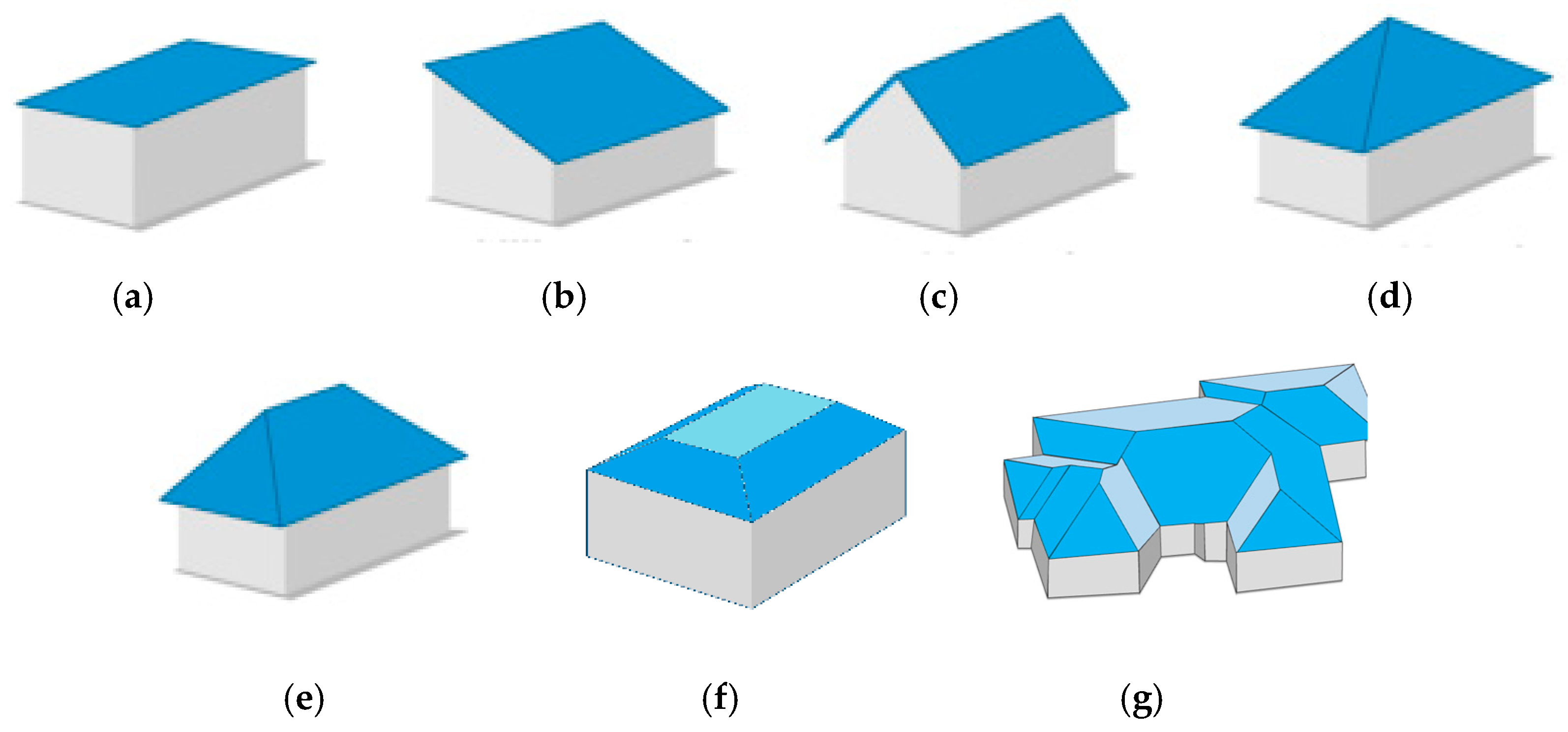
Figure 1.
Roofs model library: (a) flat; (b) shed; (c) gable; (d) pinnacle; (e) hip; (f) mansard; (g) combined.
Figure 1.
Roofs model library: (a) flat; (b) shed; (c) gable; (d) pinnacle; (e) hip; (f) mansard; (g) combined.
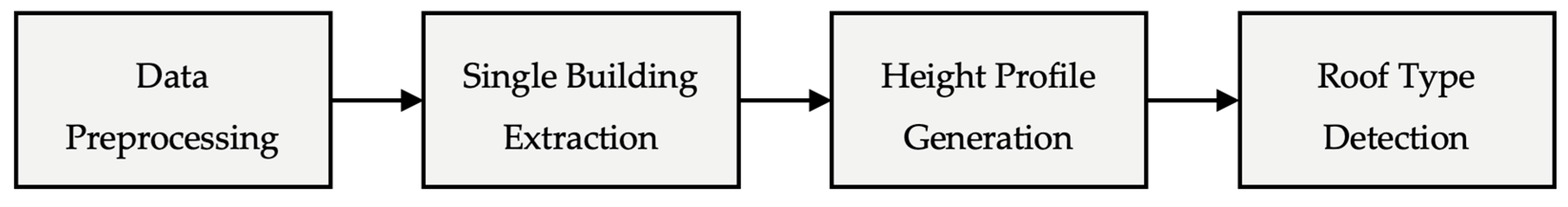
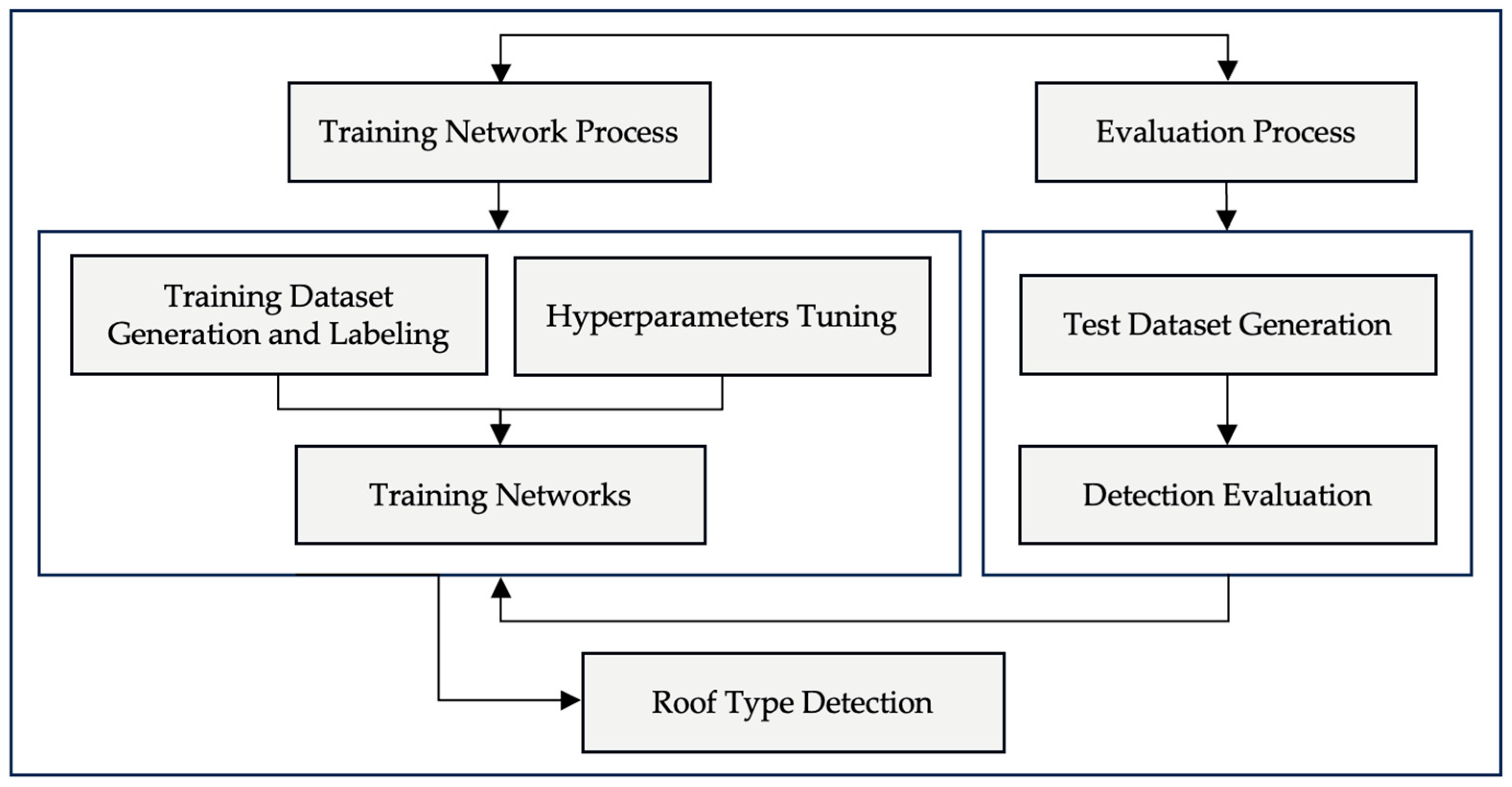
Figure 2.
The main steps of the proposed method.
Figure 2.
The main steps of the proposed method.
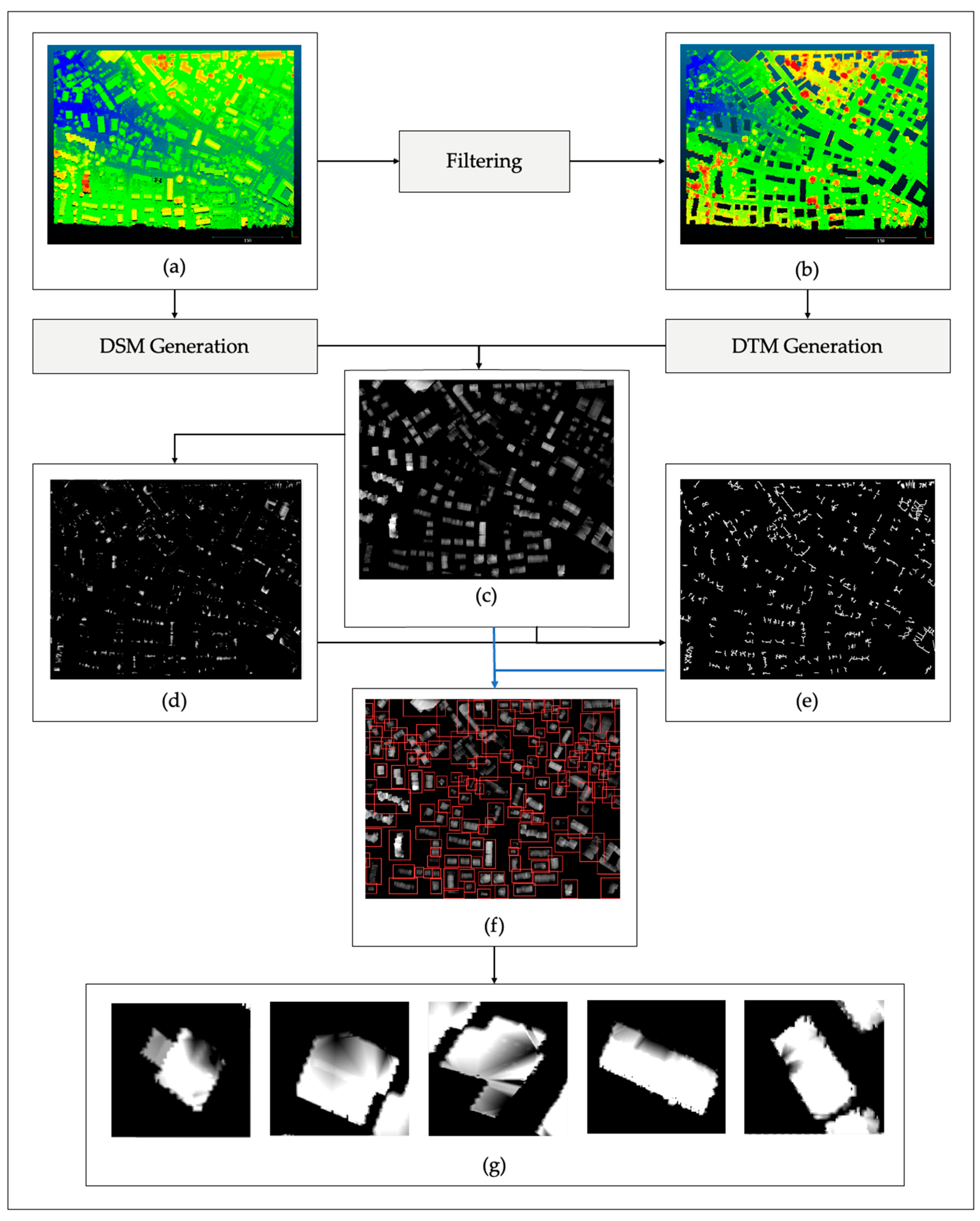
Figure 3.
The flowchart of data preprocessing, showing (a) Input LiDAR point cloud; (b) non-building point cloud; (c) generation of a normalized digital surface model (nDSM); (d) extraction of local maxima; (e) ridge line extraction; (f) extraction of sub-nDSM bounding boxes; and (g) examples of sub-nDSM segments.
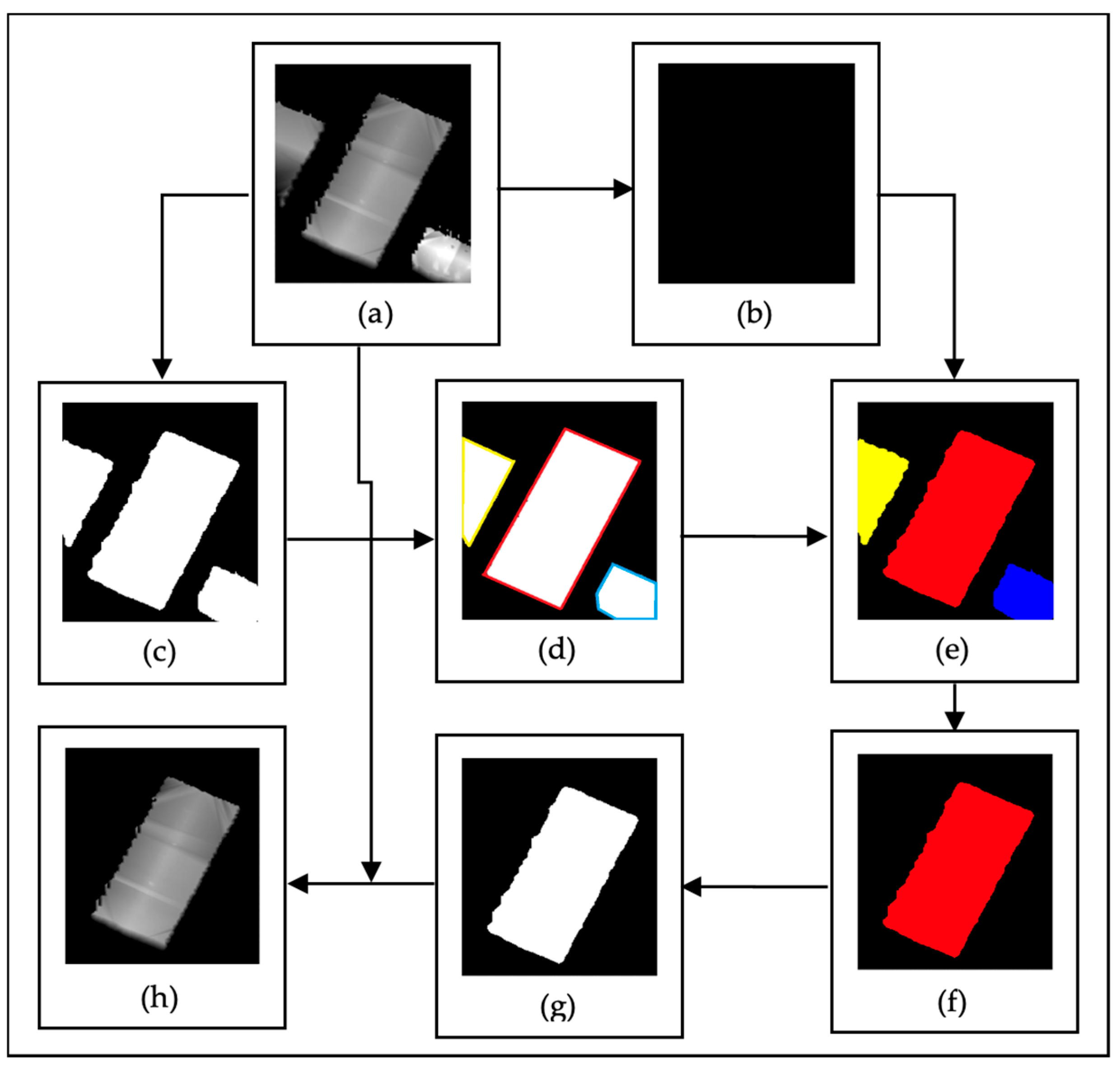
Figure 4.
The flowchart of the single building extraction process. (a) sub-nDSM. (b) null image. (c) mask image. (d) building border representation on the mask image. (e) labeled buildings in the mask image. (f) central building extraction. (g) mask image of the central building. (h) final sub-nDSM containing only the target building.
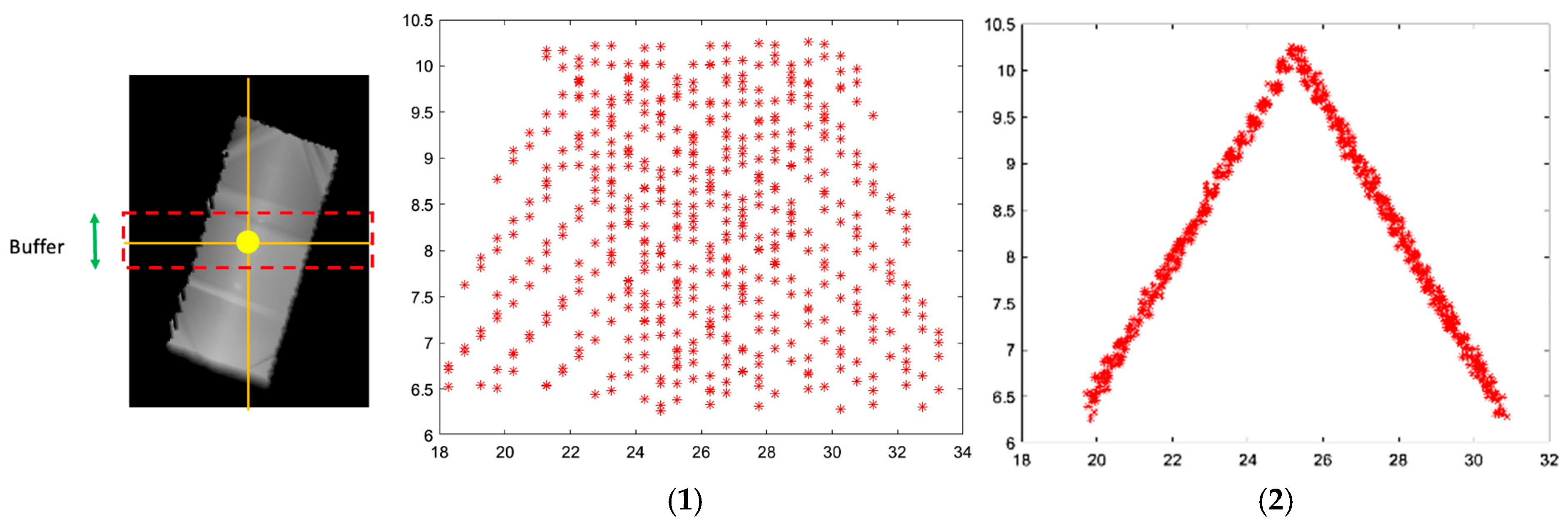
Figure 5.
Visualization of the sub-nDSM. (1) projection of the point cloud onto the XOZ plane before rotation. (2) projection of the point cloud onto the XOZ plane after applying the rotation angle.
Figure 5.
Visualization of the sub-nDSM. (1) projection of the point cloud onto the XOZ plane before rotation. (2) projection of the point cloud onto the XOZ plane after applying the rotation angle.
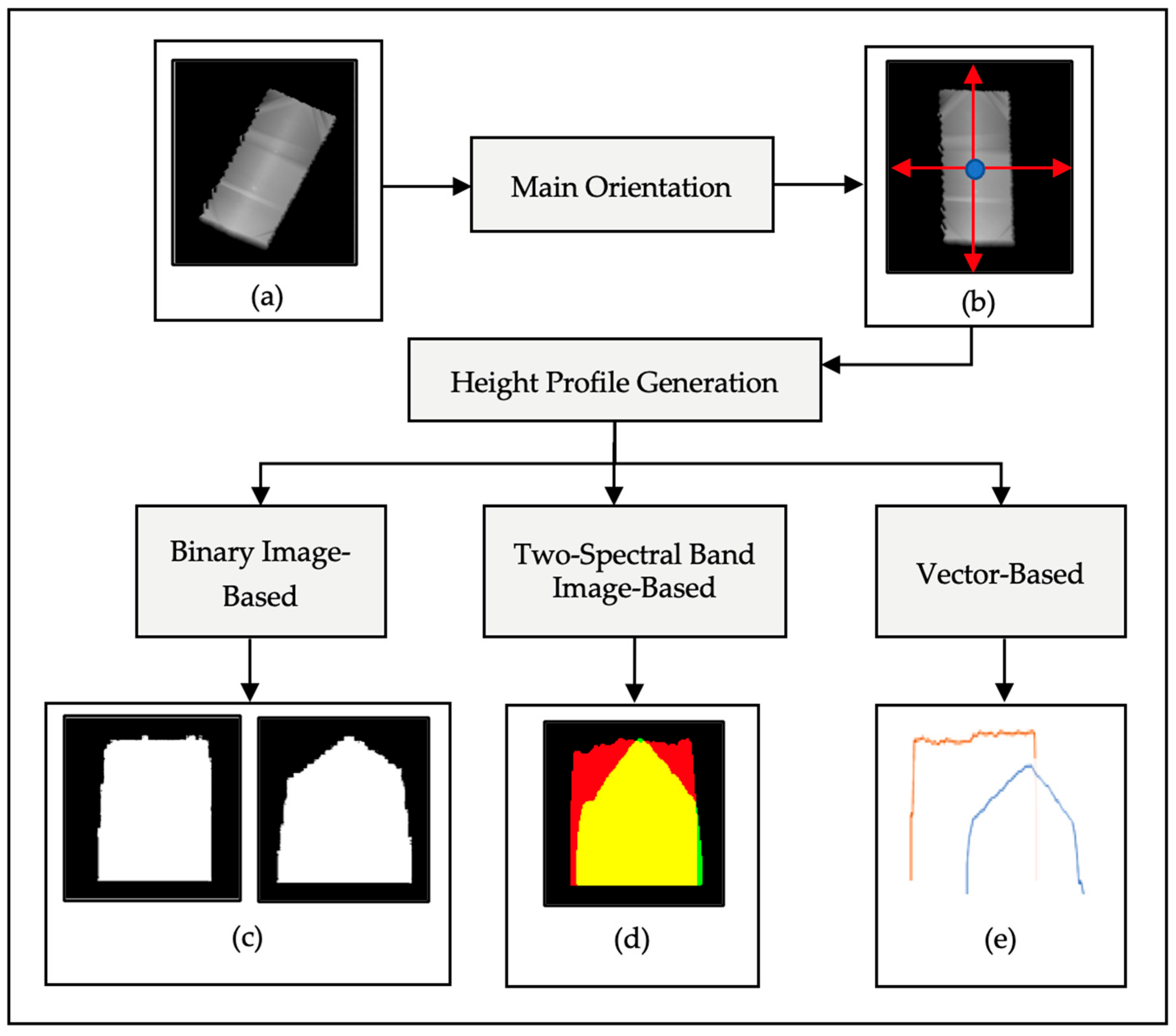
Figure 6.
The flowchart of height profile generation: (a) sub-nDSM; (b) oriented sub-nDSM; (c) first and second height profiles in binary image format; (d) height profiles in a two-spectral band image format; (e) height profiles as two 1D vectors.
Figure 6.
The flowchart of height profile generation: (a) sub-nDSM; (b) oriented sub-nDSM; (c) first and second height profiles in binary image format; (d) height profiles in a two-spectral band image format; (e) height profiles as two 1D vectors.
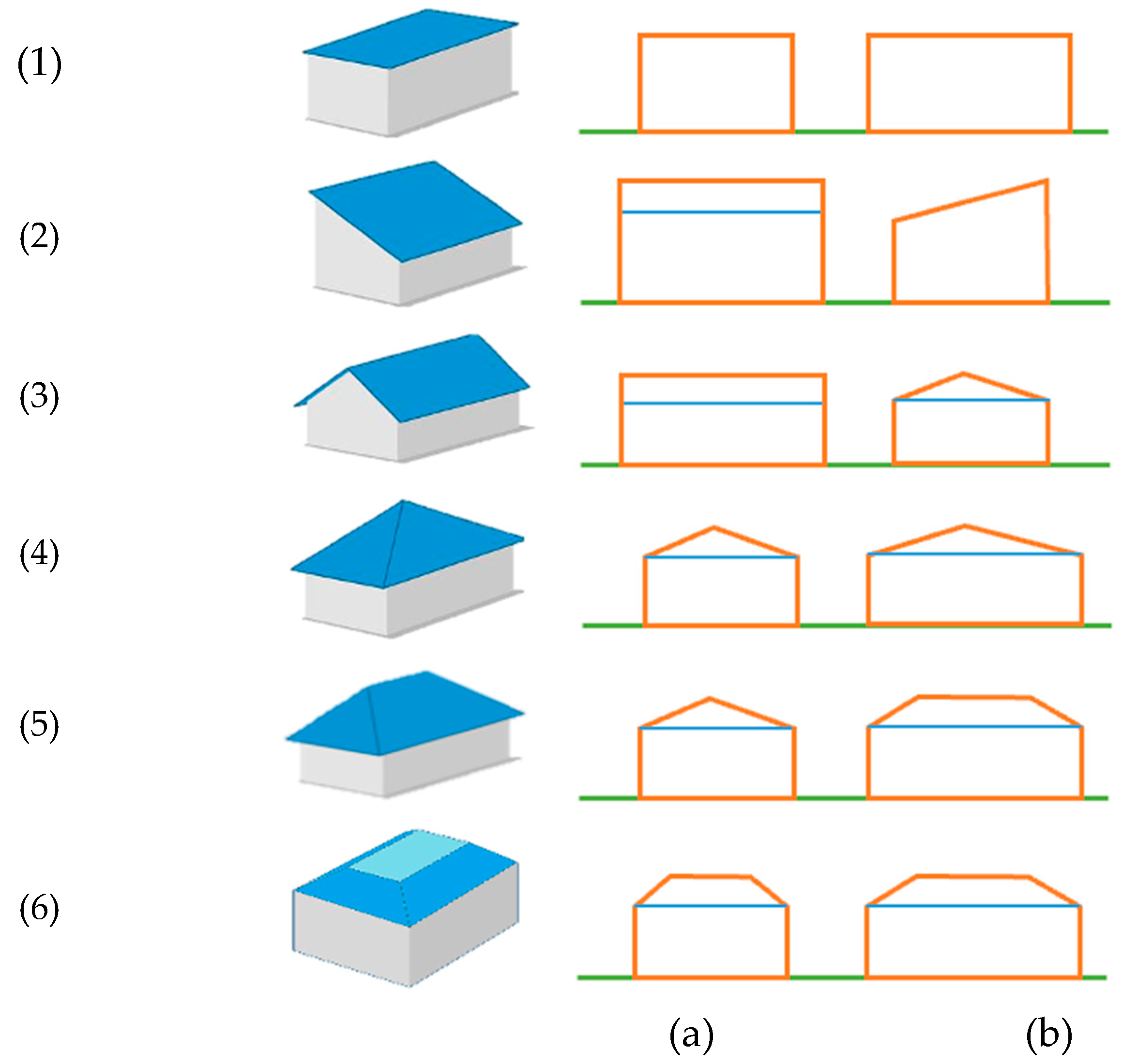
Figure 7.
Order and geometries of height profiles for various roof types: (1) flat. (2) shed. (3) gable. (4) pinnacle. (5) hip. (6) mansard. (a) the first cross-section. (b) the second cross-section.
Figure 7.
Order and geometries of height profiles for various roof types: (1) flat. (2) shed. (3) gable. (4) pinnacle. (5) hip. (6) mansard. (a) the first cross-section. (b) the second cross-section.
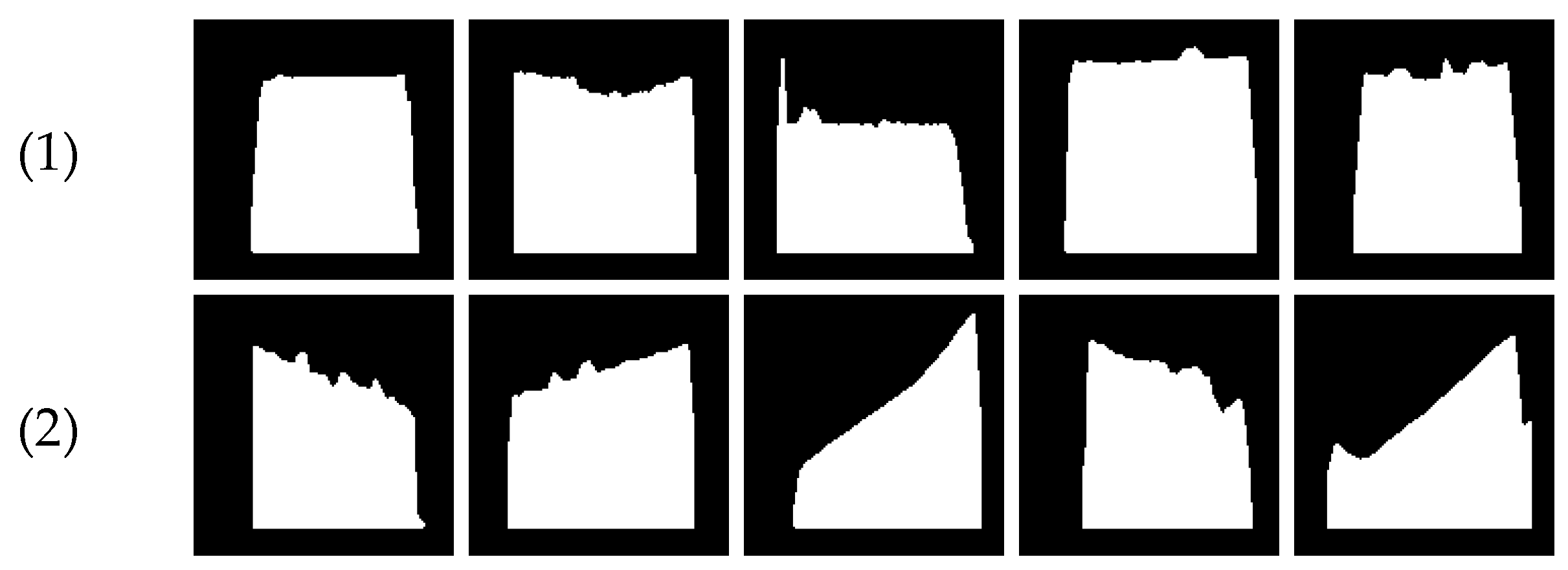
Figure 8.
Geometry type library for the binary image-based method: (1) quadrilateral. (2) convex quadrilateral. (3) pentagonal. (4) trapezoidal. (5) complex geometries.
Figure 8.
Geometry type library for the binary image-based method: (1) quadrilateral. (2) convex quadrilateral. (3) pentagonal. (4) trapezoidal. (5) complex geometries.
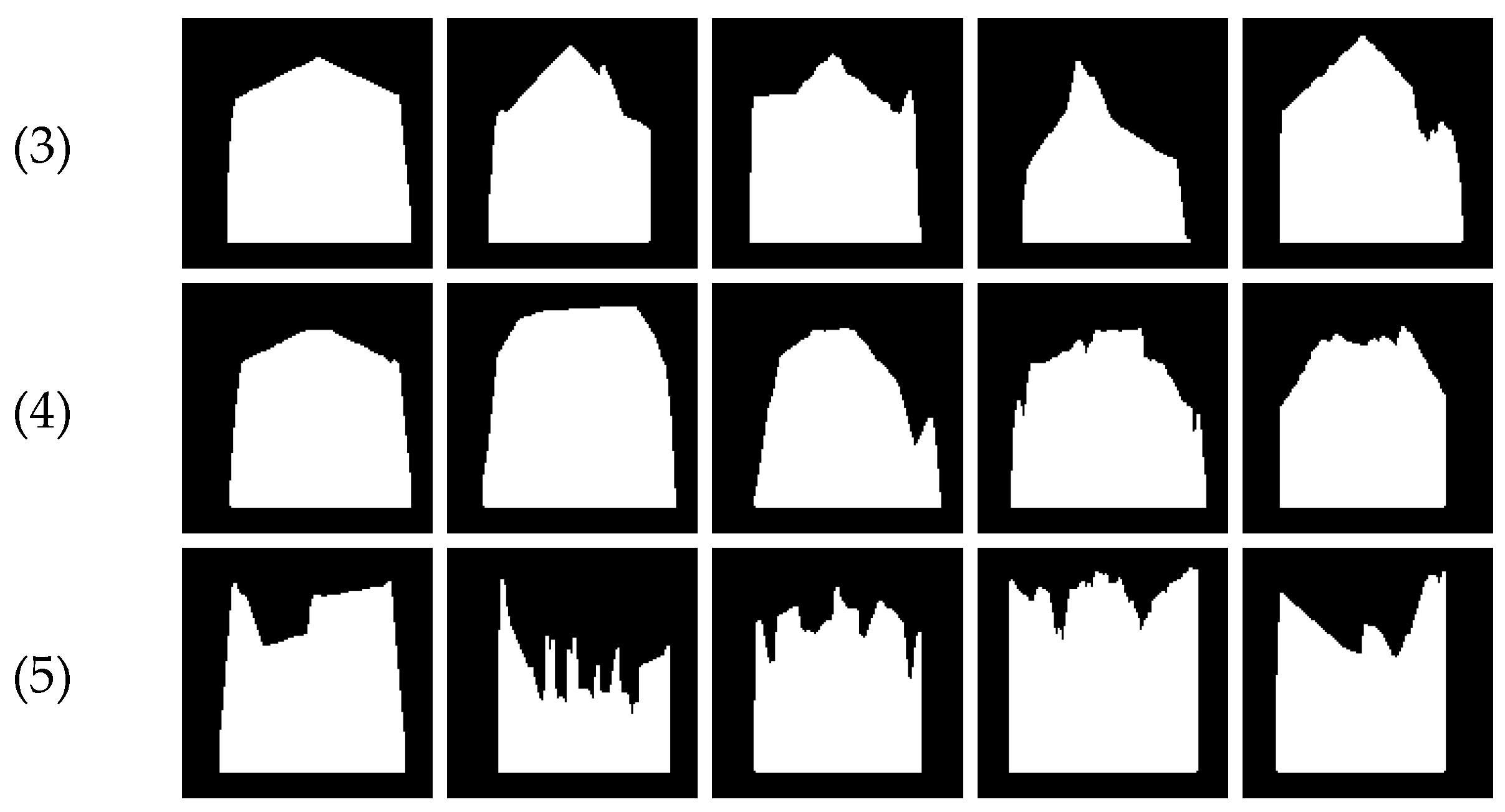
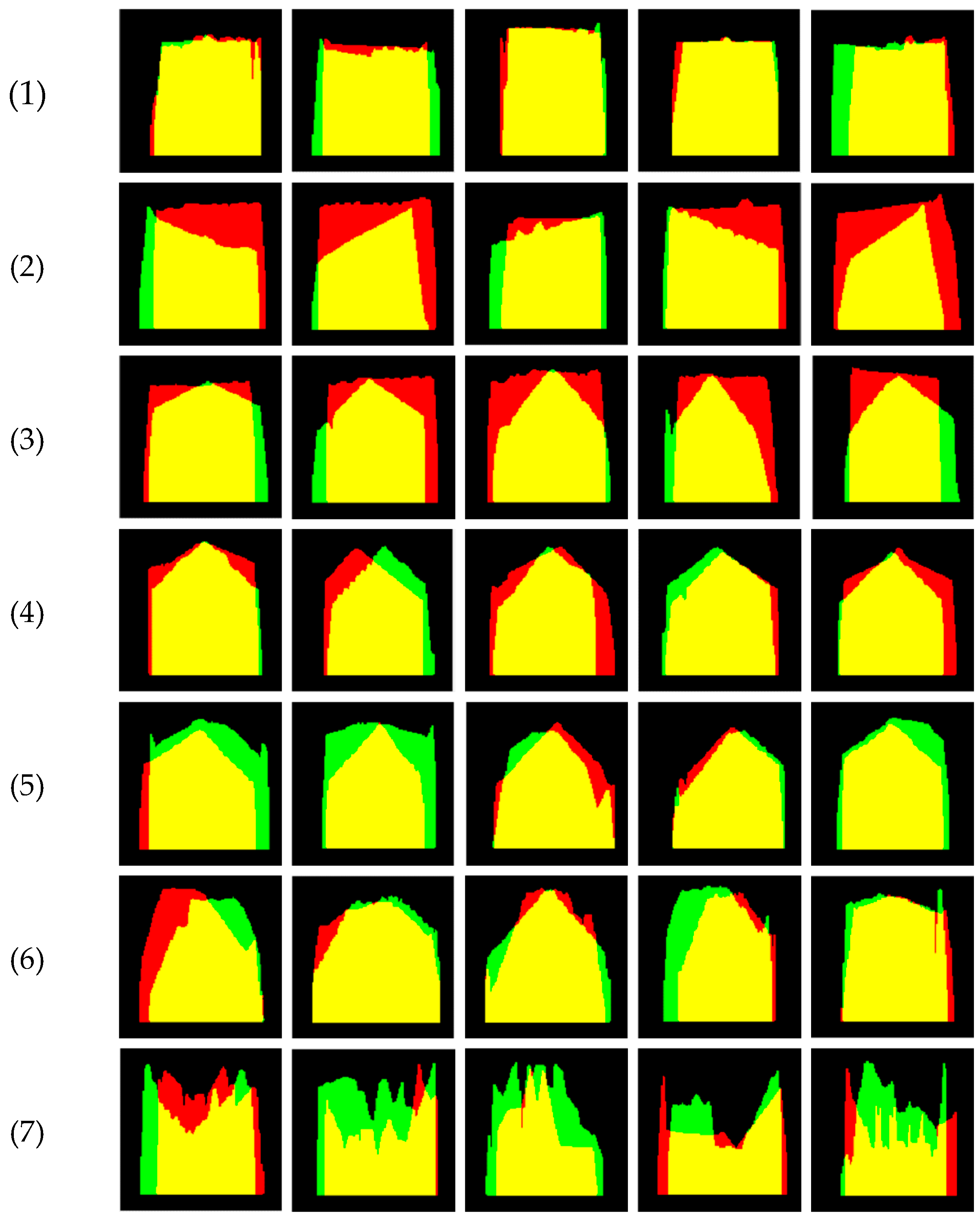
Figure 9.
Roof type library for the two-spectral band image-based method: (1) flat. (2) shed. (3) gable. (4) pinnacle. (5) hip. (6) mansard. (7) combined.
Figure 9.
Roof type library for the two-spectral band image-based method: (1) flat. (2) shed. (3) gable. (4) pinnacle. (5) hip. (6) mansard. (7) combined.
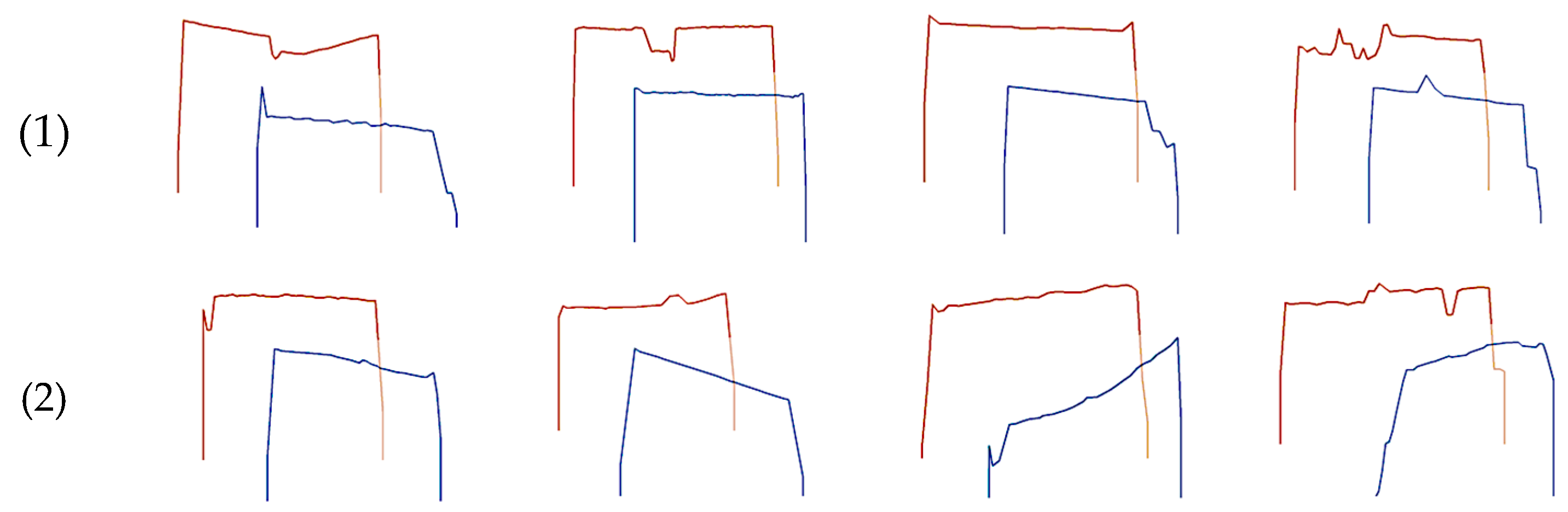
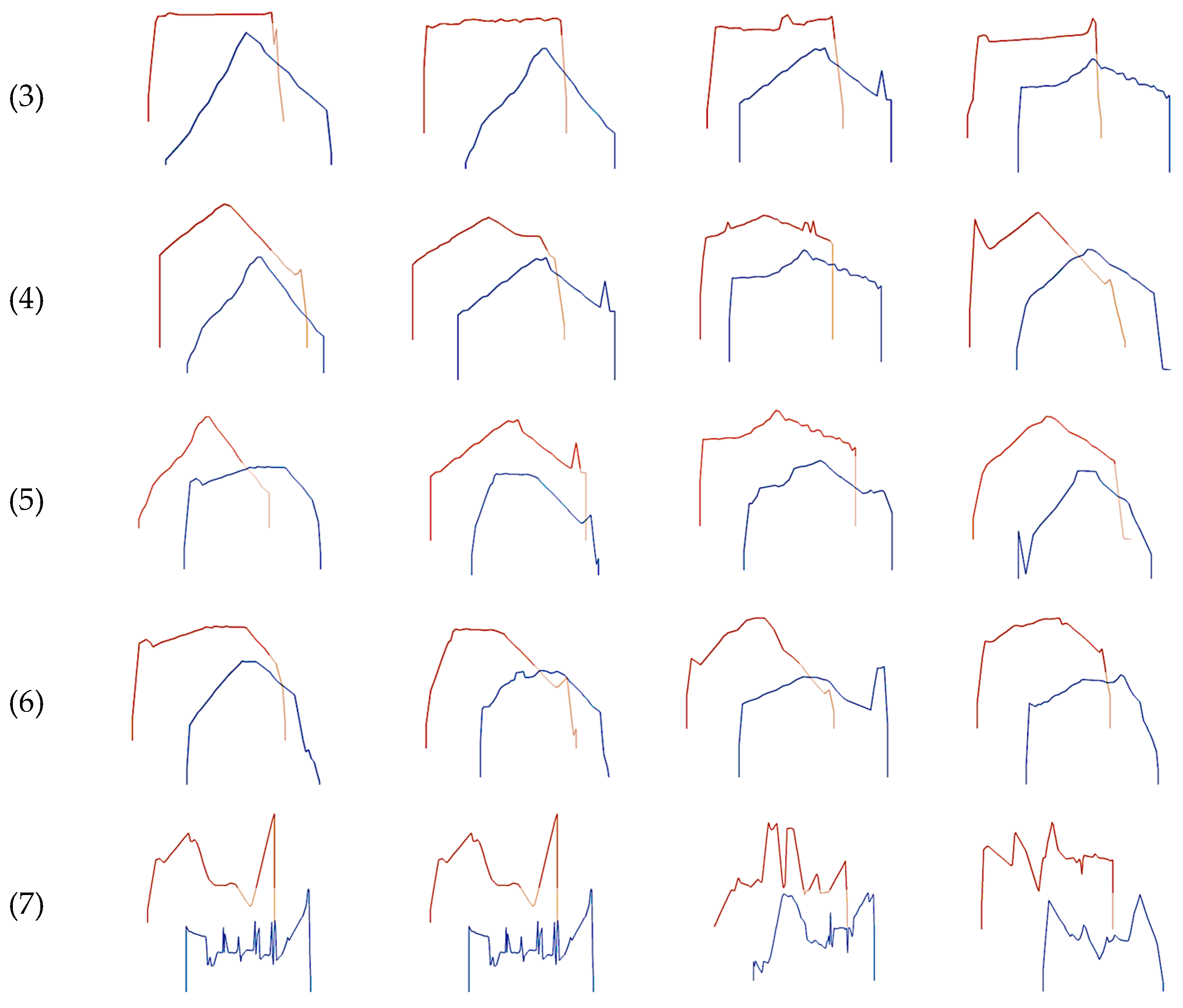
Figure 10.
Roof type library for the vector-based method: (1) flat. (2) shed. (3) gable. (4) pinnacle. (5) hip. (6) mansard. (7) combined.
Figure 10.
Roof type library for the vector-based method: (1) flat. (2) shed. (3) gable. (4) pinnacle. (5) hip. (6) mansard. (7) combined.
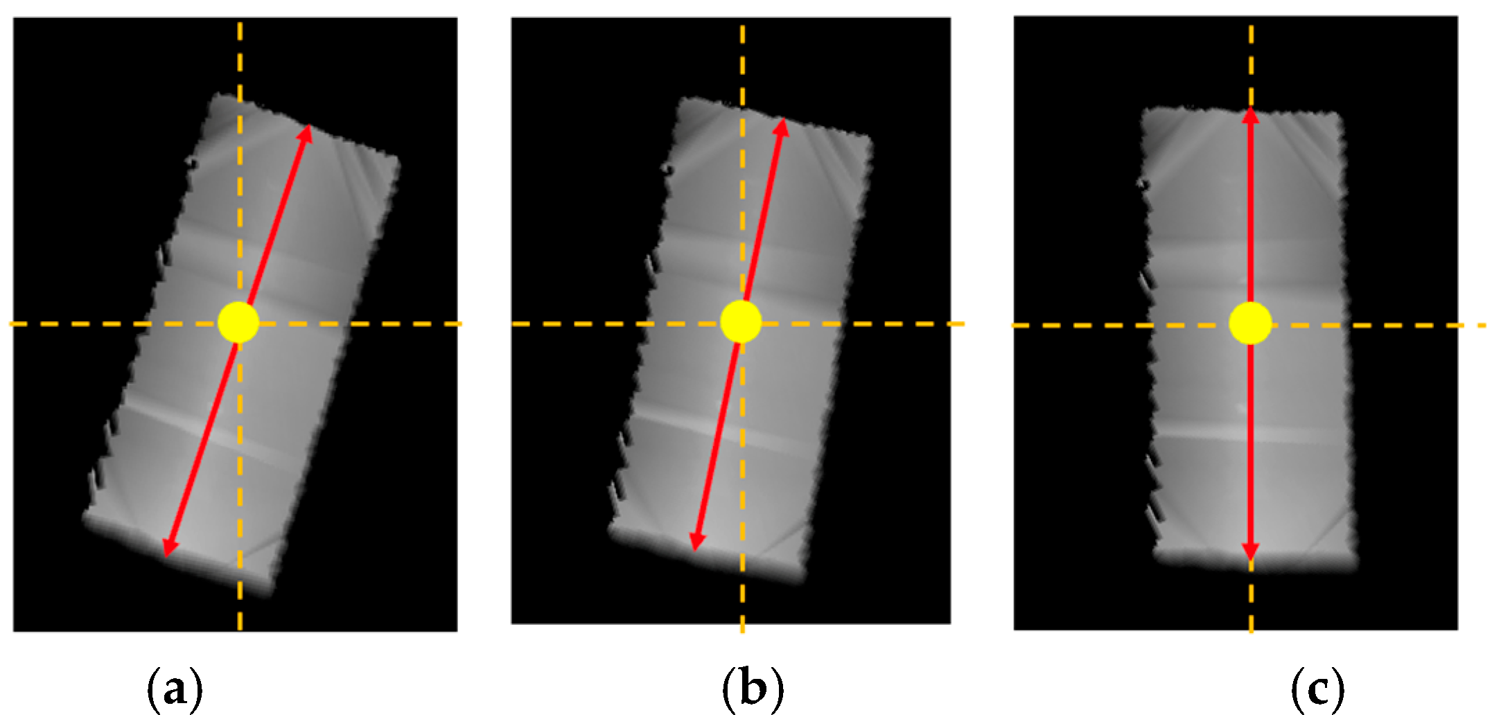
Figure 11.
Presentation of the sub-nDSM of a gable roof. (a) non-oriented sub-nDSM. (b) oriented sub-nDSM by the major orientation angle. (c) oriented sub-nDSM by both major and minor orientation angles.
Figure 11.
Presentation of the sub-nDSM of a gable roof. (a) non-oriented sub-nDSM. (b) oriented sub-nDSM by the major orientation angle. (c) oriented sub-nDSM by both major and minor orientation angles.
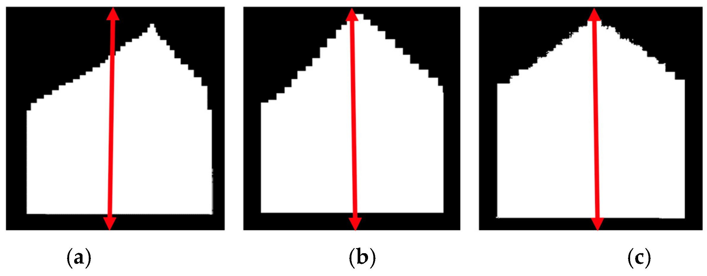
Figure 12.
Three types of height profiles with pentagonal geometry: (a) pentagonal geometry without applying a rotation angle. (b) pentagonal geometry by applying the major rotation angle. (c) pentagonal geometry by applying the major and minor rotation angles.
Figure 12.
Three types of height profiles with pentagonal geometry: (a) pentagonal geometry without applying a rotation angle. (b) pentagonal geometry by applying the major rotation angle. (c) pentagonal geometry by applying the major and minor rotation angles.
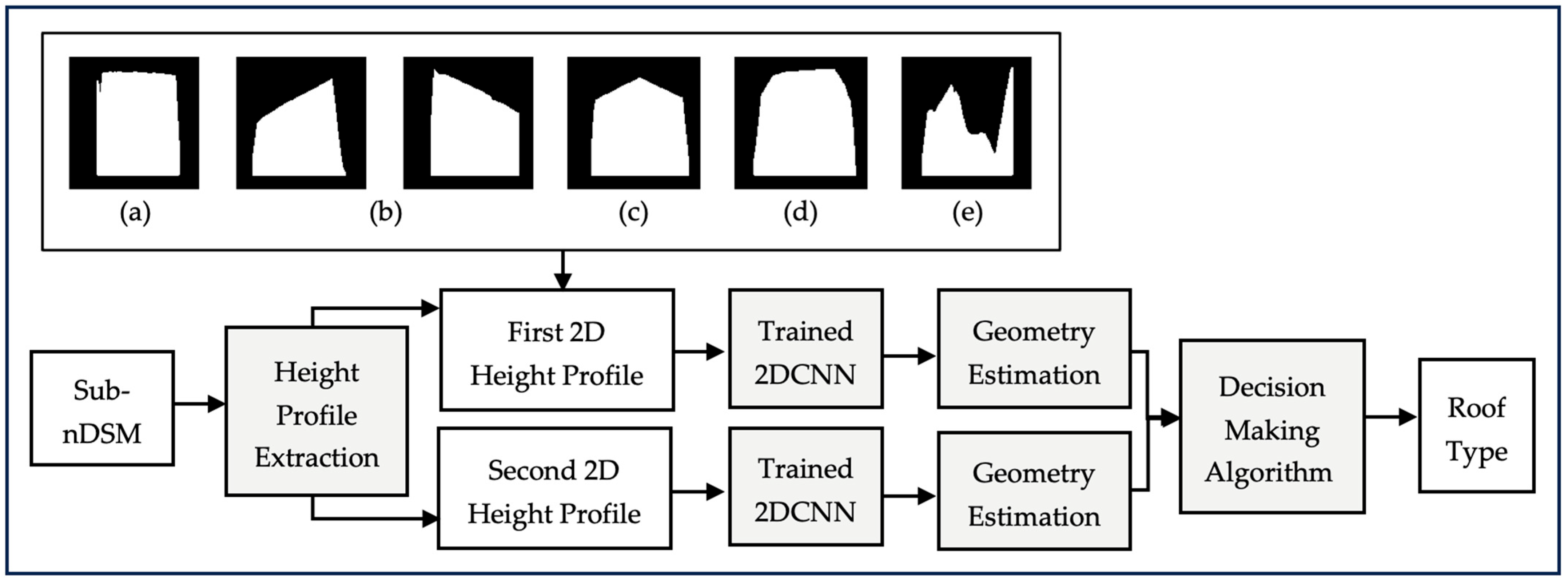
Figure 13.
Building roof type detection using height profiles.
Figure 13.
Building roof type detection using height profiles.
Figure 14.
Flowchart of roof type detection using binary image-based method: (a) quadrilateral. (b) convex quadrilateral. (c) pentagonal. (d) trapezoidal. (e) complex geometries.
Figure 14.
Flowchart of roof type detection using binary image-based method: (a) quadrilateral. (b) convex quadrilateral. (c) pentagonal. (d) trapezoidal. (e) complex geometries.
Figure 15.
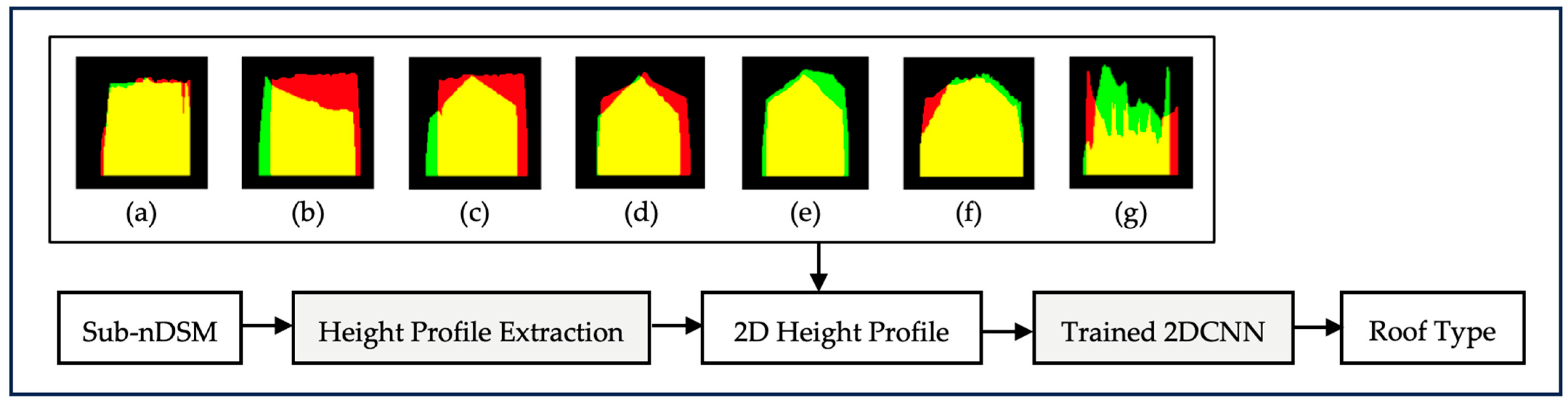
Flowchart of roof type detection using two-spectral image-based method: (a) flat. (b) shed. (c) gable. (d) pinnacle. (e) hip. (f) mansard. (g) combined roofs.
Figure 15.
Flowchart of roof type detection using two-spectral image-based method: (a) flat. (b) shed. (c) gable. (d) pinnacle. (e) hip. (f) mansard. (g) combined roofs.
Figure 16.
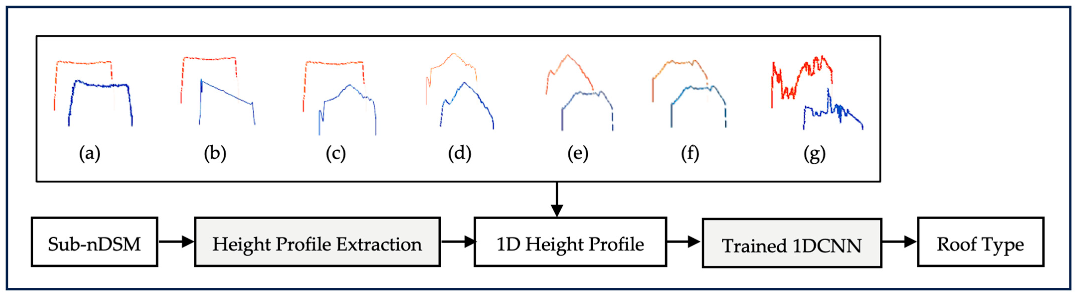
Flowchart of roof type detection using vector-based method: (a) flat. (b) shed. (c) gable. (d) pinnacle. (e) hip. (f) mansard. (g) combined roofs.
Figure 16.
Flowchart of roof type detection using vector-based method: (a) flat. (b) shed. (c) gable. (d) pinnacle. (e) hip. (f) mansard. (g) combined roofs.
Figure 17.
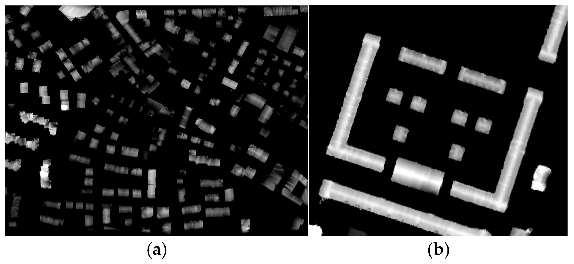
Study dataset: (a) a region of Vaihingen. (b) a region of Potsdam.
Figure 17.
Study dataset: (a) a region of Vaihingen. (b) a region of Potsdam.
Figure 18.
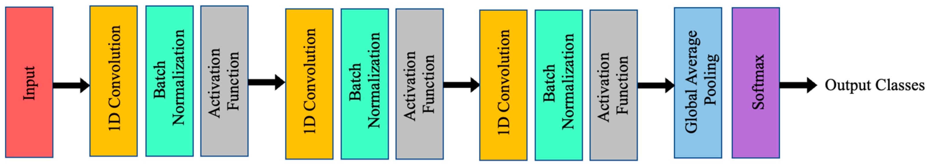
The archtiecture of the 1DCNN.
Figure 18.
The archtiecture of the 1DCNN.
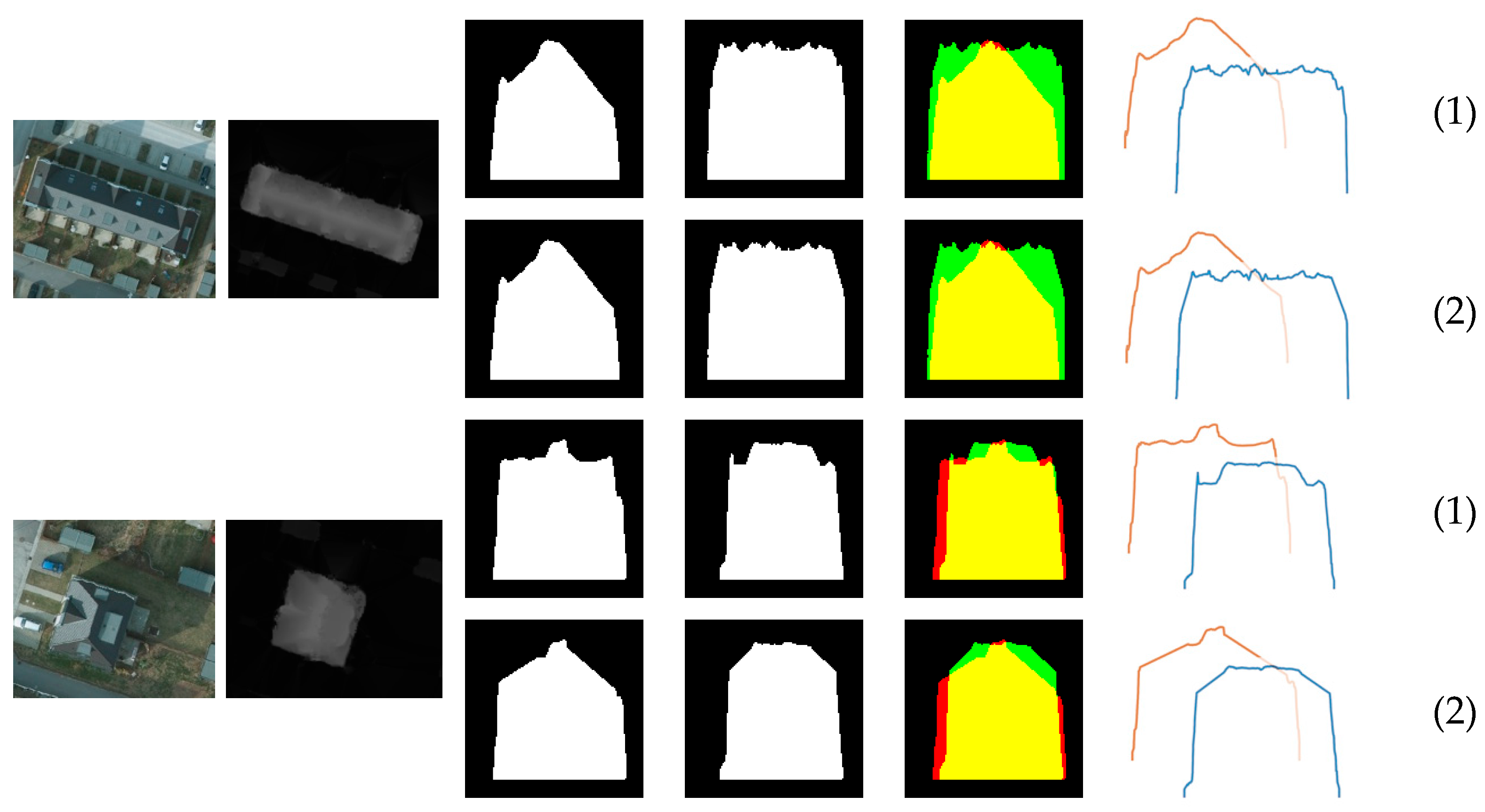
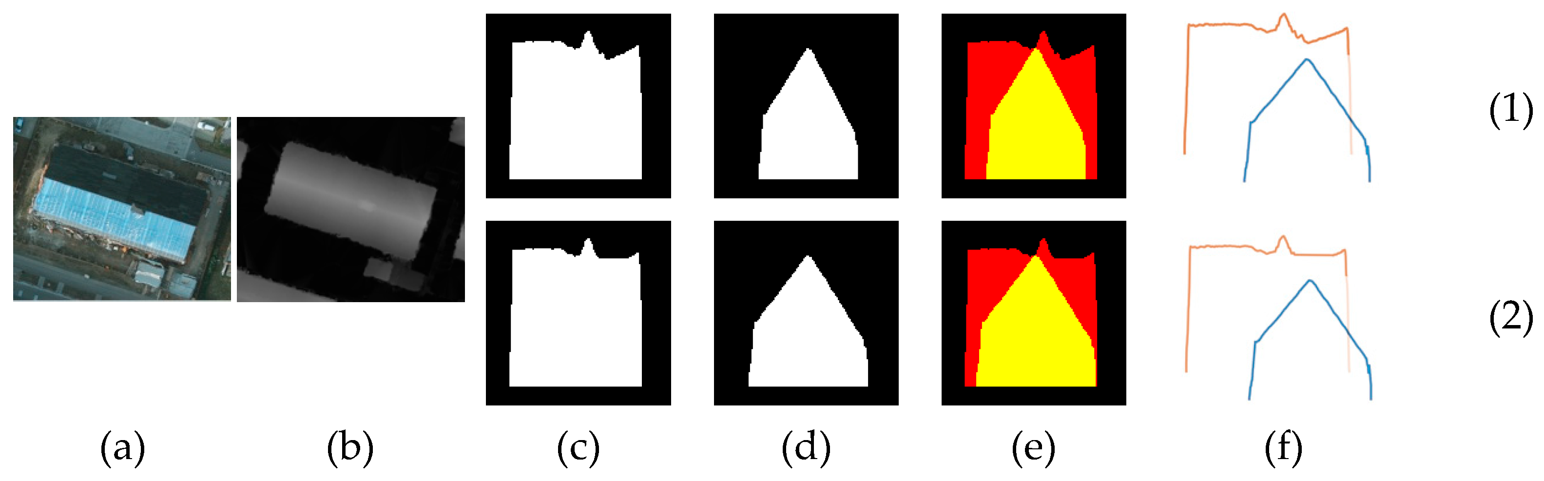
Figure 19.
View of (a) orthophoto image, (b) sub-nDSM, (c) height profiles of the first cross-section in binary image format, (d) height profiles of the second cross-section in binary image format, (e) height profiles of the cross-sections in two-spectral band image format, and (f) height profiles of the cross-sections in two 1D vectors formats. (1) with complications and noise. (2) without complications and noise.
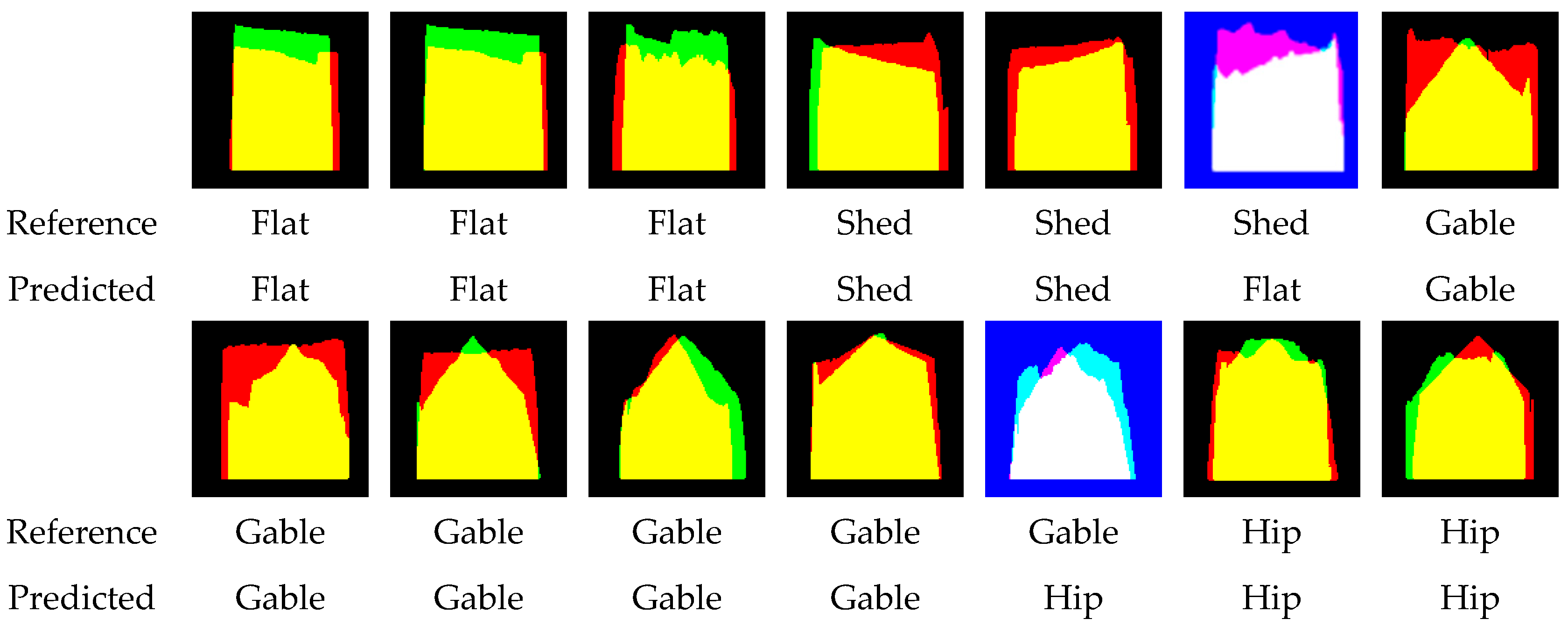
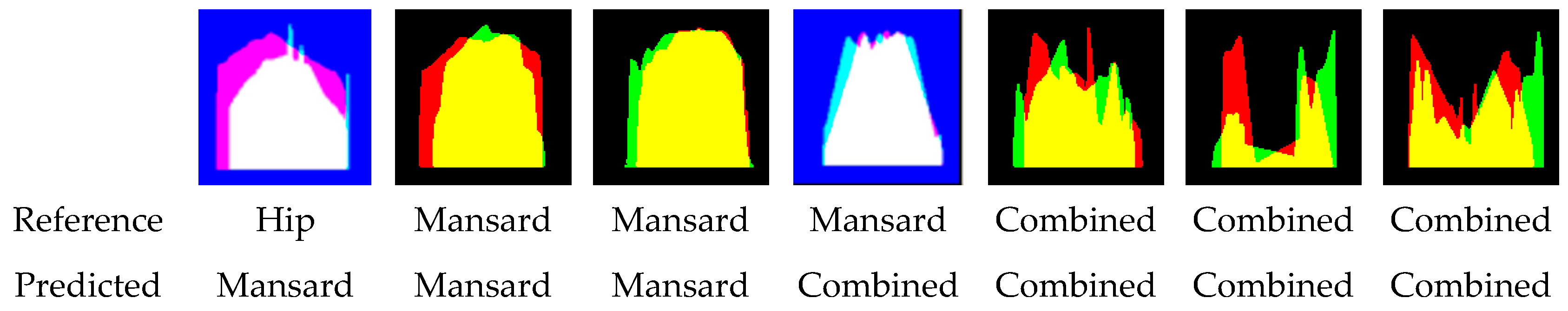
Figure 20.
Classification of seven roof types by DenseNet201.
Figure 20.
Classification of seven roof types by DenseNet201.
Table 1.
Hyperparameters used for the 2DCNN in the binary image-based method.
Table 1.
Hyperparameters used for the 2DCNN in the binary image-based method.
| 2DCNN | Optimizer | Learning Rate | Batch Size | Loss | Processing Time |
|---|
| EfficientNet-B0 | ADAM |
0.01
|
16
| 0.540 | 4 h 39 m 53 s |
| EfficientNet-B7 | ADAM |
0.001
|
16
| 0.550 | 18 h 09 m 20 s |
| DenseNet-201 | ADAM |
0.01
|
16
|
0.443
| 8 h 07 m 10 s |
| MobileNet | ADAM |
0.01
|
16
|
0.493
| 1 h 32 m 9 s |
| Inception-V3 | SGD |
0.01
|
16
| 0.480 | 4 h 15 m 16 s |
| ResNet-50 | RMSprop |
0.001
|
16
|
0.468
| 4 h 02 m 23 s |
| InceptionResNetV2 | RMSprop |
0.001
|
16
| 0.450 | 9 h 20 m 42 s |
Table 2.
Hyperparameters used for the 2DCNN in the two-spectral band image-based method.
Table 2.
Hyperparameters used for the 2DCNN in the two-spectral band image-based method.
| 2DCNN | Optimizer | Learning Rate | Batch Size | Loss | Processing Time |
|---|
| EfficientNet-B0 | ADAM | 0.01 | 16 | 0.301 | 6 h 13 m 36 s |
| EfficientNet-B7 | ADAM | 0.001 | 16 | 0.345 | 24 h 02 m 50 s |
| DenseNet-201 | RMSprop | 0.001 | 16 | 0.241 | 11 h 58 m 49 s |
| MobileNet | ADAM | 0.01 | 16 | 0.292 | 2 h 07 m 30 s |
| Inception-V3 | ADAM | 0.001 | 16 | 0.256 | 5 h 41 m 21 s |
| ResNet-50 | ADAM | 0.001 | 16 | 0.288 | 5 h 30 m 18 s |
| InceptionResNetV2 | ADAM | 0.001 | 16 | 0.233 | 12 h 31 m 31 s |
Table 3.
Hyperparameters used for the 1DCNN in the vector-based method.
Table 3.
Hyperparameters used for the 1DCNN in the vector-based method.
| 1DCNN | Optimizer | Learning Rate | Batch Size | Loss | Kernel Size | Activation Function | Processing Time |
|---|
| | ADAM | 0.001 | 32 | 0.890 | 9 | ReLU | 5 h 17 m 8 s |
Table 4.
Average results of evaluation criteria on validation data.
Table 4.
Average results of evaluation criteria on validation data.
| Methods | Neural Networks | Precision (%) | Accuracy (%) |
|---|
| Binary Image-Based Method | EfficientNet-B0 |
78.45
|
93.74
|
| EfficientNet-B7 |
77.24
|
93.7
|
| DenseNet-201 |
79.01
|
93.94
|
| MobileNet |
80.31
|
94.38
|
| Inception-V3 |
78.53
|
94.05
|
| ResNet-50 |
78.48
|
93.79
|
| InceptionResNet-V2 |
80.02
|
94.4
|
| Two-Spectral Band Image-Based Method | EfficientNet-B0 |
86.2
|
96.9
|
| EfficientNet-B7 |
85.28
|
96.46
|
| DenseNet-201 |
88.69
|
97.3
|
| MobileNet |
88.21
|
97.35
|
| Inception-V3 |
87.14
|
97.01
|
| ResNet-50 |
84.45
|
96.39
|
| InceptionResNet-V2 |
88.03
|
97.25
|
| Vector-Based Method | 1DCNN |
70.77
|
92.79
|
Table 5.
Average results of the binary image-based method on the Vaihingen test dataset.
Table 5.
Average results of the binary image-based method on the Vaihingen test dataset.
| 2DCNN | Roof Type | Geometry Type |
|---|
| Precision (%) | Recall (%) | Accuracy (%) | F1-Score (%) | IoU (%) |
|---|
| EfficientNet-B0 |
80.79
|
75.19
| 93.05 | 75.89 |
72.21
|
| EfficientNet-B7 |
87.62
|
78.18
| 96.14 | 81.90 |
80.59
|
| DenseNet-201 | 83.54 | 79.83 | 94.21 | 80.72 | 83.57 |
| MobileNet | 83.14 |
77.23
| 94.21 | 78.65 | 71.63 |
| Inception-V3 | 82.82 | 79.12 | 94.21 | 80.16 | 77.95 |
| ResNet-50 | 85.24 | 77.23 | 94.59 | 79.30 | 70.75 |
| InceptionResNet-V2 | 74.61 | 65.32 | 91.89 | 67.69 | 62.86 |
Table 6.
Average results of the two-spectral band image-based method on the Vaihingen test dataset.
Table 6.
Average results of the two-spectral band image-based method on the Vaihingen test dataset.
| 2DCNN | Roof Type |
|---|
| Precision (%) | Recall (%) | Accuracy (%) | F1-Score (%) | IoU (%) |
|---|
| EfficientNet-B0 | 75.80 |
74.47
|
92.28
|
73.85
|
59.86
|
| EfficientNet-B7 |
92.38
|
84.86
|
96.91
|
85.53
|
77.24
|
| DenseNet-201 | 86.83 | 86.51 | 96.14 | 85.86 | 76.39 |
| MobileNet | 82.62 | 82.69 | 94.60 | 81.64 | 72.38 |
| Inception-V3 | 87.70 | 87.59 | 96.91 | 87.15 | 79.09 |
| ResNet-50 | 86.05 | 86.05 | 96.14 | 85.16 | 75.95 |
| InceptionResNet-V2 | 82.26 | 82.13 | 95.37 | 81.68 | 70.50 |
Table 7.
Average results of the vector-based method on the Vaihingen test dataset.
Table 7.
Average results of the vector-based method on the Vaihingen test dataset.
| 1DCNN | Roof Type |
|---|
| Precision (%) | Recall (%) | Accuracy (%) | F1-Score (%) | IoU (%) |
|---|
|
84.52
|
84.73
|
95.37
|
83.74
| 74.01 |
Table 8.
Average results of the binary image-based method on the Potsdam test dataset.
Table 8.
Average results of the binary image-based method on the Potsdam test dataset.
| 2DCNN | Roof Type | Geometry Type |
|---|
| Precision (%) | Recall (%) | Accuracy (%) | F1-Score (%) | IoU (%) |
|---|
| Before | After | Before | After | Before | After | Before | After | Before | After |
|---|
| EfficientNet B0 |
75
|
66.67
| 62.50 |
81.25
|
61.11
|
72.23
|
53.34
|
63.46
|
54.86
| 87.50 |
| EfficientNet B7 |
50
|
66.67
|
50
|
81.25
|
50
|
72.23
|
66.67
|
63.46
|
33.33
|
89.58
|
| DenseNet201 |
75
|
66.67
|
56.25
|
81.25
|
55.56
|
72.23
|
44.45
|
63.46
| 62.50 |
89.58
|
| MobileNet |
66.67
|
66.67
|
68.75
|
87.5
|
61.11
|
77.78
|
52.28
|
67.86
|
64.58
|
100
|
| InceptionV3 |
66.67
|
66.67
|
68.75
|
87.5
|
61.11
|
77.78
|
52.28
|
67.86
|
64.58
|
91.67
|
| ResNet50 |
75
|
66.67
|
56.25
|
81.25
|
55.56
|
72.23
|
44.45
|
63.46
|
52.78
|
89.58
|
| InceptionResNetV2 |
75
|
66.67
| 62.50 |
81.25
|
61.11
|
72.23
|
53.34
|
63.46
|
81.25
|
89.58
|
Table 9.
Average results of the two-spectral band image-based method on the Potsdam test dataset.
Table 9.
Average results of the two-spectral band image-based method on the Potsdam test dataset.
| 2DCNN | Roof Type |
|---|
| Precision (%) | Recall (%) | Accuracy (%) | F1-Score (%) | IoU (%) |
|---|
| Before | After | Before | After | Before | After | Before | After | Before | After |
|---|
| EfficientNet B0 | 100 |
100
| 68.75 |
93.75
| 72.22 |
94.45
| 77.28 |
96.67
| 68.75 | 93.75 |
| EfficientNet B7 | 100 |
100
| 68.75 |
93.75
| 72.22 |
94.45
| 77.28 |
96.67
| 68.75 | 93.75 |
| DenseNet201 | 100 |
100
| 100 |
100
| 100 |
100
| 100 |
100
| 100 |
100
|
| MobileNet | 100 |
100
| 68.75 |
100
| 72.22 |
100
| 77.28 |
100
| 68.75 |
100
|
| InceptionV3 | 100 |
100
| 75 |
100
| 77.78 |
100
| 83.34 |
100
| 75 |
100
|
| ResNet50 | 100 |
100
| 75 |
75
| 77.78 |
77.78
| 83.34 |
83.34
| 75 | 75 |
| InceptionResNetV2 | 100 |
100
| 81.25 |
93.75
| 83.34 |
94.45
| 88.46 |
96.67
| 81.25 | 93.75 |
Table 10.
Average results of the vector-based method on the Potsdam test dataset.
Table 10.
Average results of the vector-based method on the Potsdam test dataset.
| 1DCNN | Roof Type |
|---|
| Precision (%) | Recall (%) | Accuracy (%) | F1-Score (%) | IoU (%) |
|---|
| Before | After | Before | After | Before | Before | After | Before | After | Before |
|---|
|
50
|
50
|
50
|
50
|
55.56
|
50
|
50
|
50
|
50
|
55.56
|
Table 11.
Average results of the Densenet201 on the test dataset, separated by each class.
Table 11.
Average results of the Densenet201 on the test dataset, separated by each class.
| Dataset | Roof Type | TP | TN | FP | FN | IoU (%) | Precision (%) | Recall (%) | Accuracy (%) | F1-Score (%) |
|---|
| Vaihingen Test Dataset | Flat | 4 | 32 | 1 | 0 | 80 | 80 | 100 | 97.30 | 88.89 |
| Shed | 4 | 32 | 0 | 1 | 80 | 100 | 80 | 97.30 | 88.89 |
| Gable | 5 | 32 | 0 | 0 | 100 | 100 | 100 | 100 | 100 |
| Pinnacle | 5 | 30 | 0 | 2 | 71.43 | 100 | 71.43 | 94.59 | 83.33 |
| Hip | 7 | 27 | 2 | 1 | 70 | 77.78 | 87.50 | 91.89 | 82.35 |
| Mansard | 2 | 33 | 1 | 1 | 50 | 66.67 | 66.67 | 94.59 | 66.67 |
| Combined | 5 | 31 | 1 | 0 | 83.33 | 83.33 | 100 | 97.30 | 90.91 |
| Potsdam Test Dataset | Gable | 1 | 8 | 0 | 0 | 100 | 100 | 100 | 100 | 100 |
| Hip | 8 | 1 | 0 | 0 | 100 | 100 | 100 | 100 | 100 |
| Average | 81.64 | 89.75 | 89.51 | 97 | 89 |


