PDAA: An End-to-End Polygon Dynamic Adjustment Algorithm for Building Footprint Extraction

Abstract

Buildings are a significant component of urban space and are essential to smart cities, catastrophe monitoring, and land use planning. However, precisely extracting building polygons from remote sensing images remains difficult because of the variety of building designs and intricate backgrounds. This paper proposes an end-to-end polygon dynamic adjustment algorithm (PDAA) to improve the accuracy and geometric consistency of building contour extraction by dynamically generating and optimizing polygon vertices. The method first locates building instances through the region of interest (RoI) to generate initial polygons, and then uses four core modules for collaborative optimization: (1) the feature enhancement module captures local detail features to improve the robustness of vertex positioning; (2) the contour vertex tuning module fine-tunes vertex coordinates through displacement prediction to enhance geometric accuracy; (3) the learnable redundant vertex removal module screens key vertices based on a classification mechanism to eliminate redundancy; and (4) the missing vertex completion module iteratively restores missed vertices to ensure the integrity of complex contours. PDAA dynamically adjusts the number of vertices to adapt to the geometric characteristics of different buildings, while simplifying the prediction process and reducing computational complexity. Experiments on public datasets such as WHU, Vaihingen, and Inria show that PDAA significantly outperforms existing methods in terms of average precision (AP) and polygon similarity (PolySim). It is at least 2% higher than existing methods in terms of average precision (AP), and the generated polygonal contours are closer to the real building geometry. Values of 75.4% AP and 84.9% PolySim were achieved on the WHU dataset, effectively solving the problems of redundant vertices and contour smoothing, and providing high-precision building vector data support for scenarios such as smart cities and emergency response.

1. Introduction

Buildings are a fundamental component of urban structure and are essential to land use, environmental monitoring, disaster assessment, transportation planning, and other domains. The advancement of remote sensing technology offers a new method for highly accurate and large-scale building information collection. We can accomplish dynamic monitoring of urban spatial morphology and supply essential data support for smart city development and emergency response by extracting building contours from remote sensing images. However, the complicated background information, dense distribution, and varied appearance of buildings make it difficult to develop an efficient automatic building footprint extraction method. Traditionally, building contour extraction relies on a series of rule-based image processing techniques, including edge detection, threshold segmentation, morphological operations, region growing, watershed transform, etc. These methods mainly rely on the brightness changes, color, or texture features of the image to distinguish buildings from other objects. In recent years, with the rapid development of deep neural networks and the increasing abundance of building annotation data, building extraction methods based on deep learning have become mainstream and have been widely used and explored in many fields such as remote sensing, geographic information systems (GISs), and computer vision [1,2,3,4,5]. However, considerable regional variations in building color, shape, area, and material, as well as the high similarity and hazy boundaries between buildings and other landforms in remote sensing images, make it difficult to automatically and accurately extract building contours from these images [6].

Most deep learning-based studies formulate building extraction as a pixel semantic labeling task. Each pixel is classified as “building” or “non-building” according to a carefully designed network architecture. Even though they perform well when creating binary segmentation masks, turning these masks into a set of building polygons needed for mapping and geographic applications is difficult. Although post-processing and regularization procedures can help these pixel-based methods generate higher quality building polygons [7,8], due to the separation of segmentation and regularization procedures, such methods usually need to train multiple separate models for segmentation, regularization, and vectorization [9]. These models are ineffective and complicated, and mistakes are made all along the way. The produced polygons’ application in real engineering is limited since they have incorrect edges and differ greatly from the actual building contours (Figure 1b).

To meet the demands of practical applications in geospatial analysis, contour-based techniques [10,11,12] have emerged as an alternative to pixel-by-pixel segmentation, directly predicting the polygon of each building instance. Existing contour-based methods can be broadly categorized into two approaches. The first approach [10,11,12,13] constructs building polygons by predicting the precise coordinates and sequential arrangement of building vertices. Its core challenge lies in accurately determining both vertex positions and their ordering to form a polygon that faithfully represents the building’s geometry. Typically employing convolutional neural networks (CNNs), this approach detects all building corners across the input image and infers their connection order to form the polygon, offering a conceptually straightforward framework. However, it frequently suffers from missed corner detections, particularly for inconspicuous vertices, sometimes leading to entire building instances being overlooked (Figure 1c). Moreover, an incorrect prediction of one vertex often propagates errors to subsequent vertices, compromising the overall polygon quality. Crucially, the lack of an effective compensation mechanism limits its ability to represent irregular building shapes accurately. Additionally, the requirement for pixel-level vertex and direction prediction often necessitates complex models with higher parameter counts and longer inference times.

The second approach [14,15,16,17] initializes a fixed number of ordered polygon vertices and iteratively optimizes their positions to converge on the final building polygon. While simplifying the problem formulation, this method overlooks the inherent geometric diversity of buildings. Specifically, vertex positions are refined through iterative coordinate regression. A significant drawback is that the preset, fixed vertex count is inherently mismatched to the variable complexity of building outlines. This results in redundant vertices for simple buildings and insufficient vertices for complex ones (Figure 1d). Furthermore, these methods lack mechanisms to prune redundant points or prioritize key vertices, often leading to overly smoothed polygons. This excessive smoothing obscures critical geometric features such as right angles and sharp edges, diminishing the fidelity of the representation. Particularly for buildings with intricate internal structures or unusual geometries, this smoothing tendency can cause significant divergence between the predicted polygon and the actual building contour.

To address the aforementioned limitations, this paper proposes an end-to-end polygon dynamic adjustment algorithm (PDAA). PDAA is designed to adapt to complex and varied building shapes while reducing reliance on large-scale labeled data and maintaining low inference latency. Furthermore, it aims to enhance both the accuracy and geometric fidelity of the predicted building polygons. Our approach initially concentrates on localized regions of interest (RoIs). Leveraging the detection head of a deep learning model, we predict a set of building bounding boxes based on the feature map derived from the input image. These bounding boxes pinpoint the location of individual buildings. Crucially, a variable number of polygon vertices is then generated per instance to construct the initial building polygon. This strategy enables the capture of a building’s general structure while accommodating structures of diverse sizes and shapes.

PDAA incorporates four specialized modules: (1) Feature Enhancement Module: This focuses on capturing key feature points within the RoI, thereby deepening the model’s understanding of specific building details and refining polygon generation accuracy. (2) Contour Vertex Adjustment Module: This operates on the initial polygon vertices within the proposal. It extracts detailed coordinate information, encodes instance-specific features into the RoI features, and learns to predict displacements for each vertex, relocating them to more accurate positions. (3) Learnable Redundant Vertex Removal Module: This functions as a corner point classifier, specifically tasked with distinguishing true corner points from redundant ones and eliminating the latter. This ensures that the final polygon comprises only essential vertices, enhancing its quality and geometric consistency. (4) Missing Vertex Completion Module: This iteratively optimizes the positions of incorrectly predicted vertices, gradually recovering overlooked key feature points. This mechanism guarantees the generation of high-precision polygons, even for complex structures or small building features.

In summary, the main contributions of this paper include the following:

(1)

We propose an end-to-end contour-based polygon dynamic adjustment algorithm (PDAA) for high-quality building contour extraction. The framework combines efficient reasoning with high precision. Through the dynamic vertex optimization mechanism driven by contour features, the regularized building contour consisting of key corner points is directly generated, achieving high precision and efficiency in building contour extraction.

(2)

A deep learning model is applied to generate the initial polygons, and a technique that concentrates on local features within the RoI is proposed. The prediction accuracy and geometric similarity are significantly improved through four core modules (feature enhancement, contour vertex adjustment, redundant vertex removal, and missing vertex completion).

(3)

The prediction process is simplified, the computational complexity and running time are reduced, and polygon vertices are adaptively generated according to different building instances, making the prediction results closer to the geometric characteristics of real buildings, significantly improving the accuracy and visual effects.

2. Related Work

2.1. Pixel-by-Pixel Methods for Building Footprint Extraction

Extracting building footprints from satellite or aerial images has been widely studied for decades. Traditional building extraction methods include shadow index-based [18], edge regularity-based [19], or line segment-based [20] methods. This type of method relies on manual features and prior knowledge and has certain applicability in specific scenarios, but it has weak generalization ability in complex remote sensing images. Recently, most studies on building footprint extraction have been based on deep learning methods for pixel-level semantic labeling. Semantic segmentation models such as U-Net [21], FC-DenseNet [22], high-resolution network (HR-Net) [23], and instance segmentation models such as Mask-RCNN [24] have been widely explored and have achieved effective building extraction results. In particular, after the success of U-Net in medical image segmentation, it was quickly introduced into the remote sensing field and became the basic architecture for many subsequent works. Its advantage is that it retains spatial information through skip connections and is suitable for processing fine-grained targets in high-resolution remote sensing images. In addition, instance segmentation models such as Mask R-CNN are also used in building extraction tasks, which can achieve detection and segmentation at the same time and are suitable for building recognition in multi-object scenes. With the rapid development of remote sensing image semantic segmentation technology, a series of advanced models based on the Transformer architecture and multi-scale feature fusion have been proposed, such as TransUNet [25], GPINet [26], and RSMamba [27]. They used attention mechanism and sequence modeling structure to optimize the multi-scale feature extraction process of remote sensing images, respectively. These models enhance the adaptability to complex remote sensing scenes and improve segmentation accuracy. There are also some works that try to improve the boundary quality by improving the loss function or introducing auxiliary strategies. Guo et al. [28] proposed a coarse-to-fine network based on the U-Net architecture to gradually refine the building boundaries of different scales. Wu et al. [29] proposed a terrain-aware loss based on a high-resolution network architecture to improve the network’s ability to preserve building segmentation boundaries. In addition, various useful strategies, such as data fusion [1,30,31], distance transformation [32], and boundary regularization [7,8], are combined with the pixel-by-pixel segmentation network to further improve the building segmentation performance. Although CNN-based pixel-by-pixel methods have achieved increasingly high prediction accuracy, the building extraction results produced by these methods are often very different from the polygonal buildings required in practical applications. The contours of building footprints predicted by these methods are curved shapes, while the actual building polygons are manually annotated in a line-based manner with a relatively small number of edges and vertices. Processing the prediction results of these methods into the required building polygons in vector format usually requires heavy work. Although these pixel-based methods achieve great results in terms of building area coverage, they show inefficiency in inferring the overall shape of buildings, limiting their applicability in practical engineering.

2.2. Contour-Based Methods for Building Footprint Extraction

To address the demands of real-world applications, a number of contour-based methods have been put out to produce building polygons directly. Polygon-RNN [33] and Polygon-RNN++ [13] are among the earliest works to propose such a framework. They use a recurrent neural network (RNN) structure to sequentially predict the vertices of a polygon given a true bounding box. This design is the first to achieve an end-to-end polygon generation process, but its reliance on manually annotated bounding boxes limits its practicality. PolyMapper [12] extended this architecture by adding a pre-process object detection module. It uses a feature pyramid network (FPN) architecture to predict building bounding boxes [34] and then uses a ConvLSTM model to sequentially predict building corners within the extracted bounding boxes [35]. Zhao et al. [3] further improved PolyMapper by upgrading the detection module and the RNN part. The CNN-RNN paradigm is inefficient in training and inference due to its complex architecture and beam search process, respectively. Compared with the Polygon-RNN method [13,33], Curve-GCN [36] uses a graph convolutional network (GCN) to predict all polygon vertices at once and model the topological relationship between vertices through a graph structure. This method avoids the sequential dependency of vertex generation and improves reasoning efficiency. Wei et al. [14] followed the Curve-GCN method [36] to predict the building corners at once and added a target detection module on this basis, which is more efficient. However, the limitation of the CNN-GCN paradigm is that the preset fixed number of vertices will lead to vertex redundancy. When the number of vertices set is more than what is actually required, redundant points will be generated; setting too few may cause structural distortion. Other methods [11,37] predict building polygon inflection points by performing corner detection as a segmentation task and then applying a GCN module to refine the coordinates of the previously extracted vertices. PolyWorld [11] adopts this approach and further predicts a permutation matrix to encode the connectivity information between the extracted vertices. The final polygons are subsequently created by connecting the vertices in accordance with the permutation matrix; however, during vertex segmentation, PolyWorld might not recognize building corners because of vegetation or shadows.

In summary, pixel-by-pixel segmentation methods typically yield building contours characterized by irregular, curved shapes, diverging significantly from the regular, manually annotated polygons required in practical applications. This necessitates complex and computationally intensive post-processing to convert the pixel-level results into the vector polygon format needed for architectural workflows. Contour-based methods, while addressing this format issue, often suffer from intricate network architectures that hinder training and inference efficiency. Moreover, their reliance on a fixed number of vertices frequently results in either redundant or insufficient vertices, compromising polygon accuracy.

To overcome these limitations, this paper proposes an end-to-end learnable polygon dynamic adjustment algorithm (PDAA) that seamlessly integrates building geometry understanding with the polygon deformation process. Our approach eliminates the pixel-level mask post-processing step, directly generating polygon contours that exhibit enhanced similarity to manually annotated regular polygons and directly outputting the coordinates and connectivity of polygon vertices. Crucially, PDAA adaptively generates a variable number of vertices tailored to each building’s shape.

3. Method

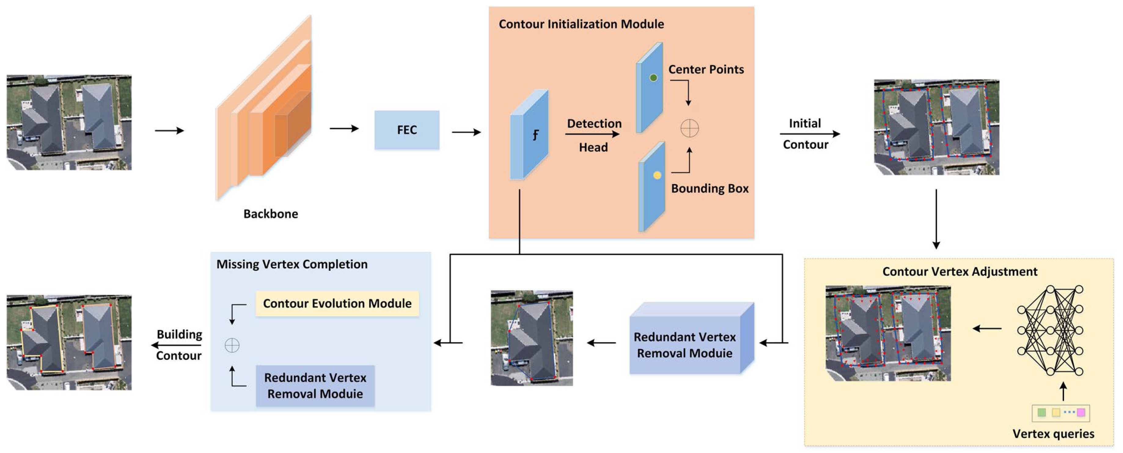
The overall process of PDAA is shown in Figure 2. The key idea of PDAA is to view the construction polygon as an extension of the bounding box and utilize four main components to generate the final prediction. Given an input image, we first apply the CNN backbone to extract the image feature map and then enhance the feature map to obtain the feature map $\mathcal{F}$. Then, we build a detection head on $\mathcal{F}$ to predict a set of building detection boxes and construct the initial contour of the building. Subsequently, PDAA generates a building polygon for each instance through three key modules: contour vertex adjustment, redundant vertex removal, and missing vertex completion. The contour vertex adjustment module predicts the offset of each point of the initial building contour to adjust the contour position, and then the redundant vertex removal module removes the redundant vertices and retains the key vertices to generate the building polygon. After that, the missing point completion module takes the building polygon and feature map $\mathcal{F}$ as input, predicts the missing building vertices, and restores the polygon with the missing vertices as the final building polygon of the instance.

3.1. Initial Contour Generation

3.1.1. Backbone

The feature map is used to identify and locate building instances and should encode semantic and spatial information. PDAA follows a convolutional neural network (CNN) based on the deep layer aggregation architecture, namely DLA [38], as the backbone network to achieve an effective fusion of low-level features with strong spatial information and high-level features rich in semantic information. The CNN backbone network structure is shown in Figure 3, which generates a feature pyramid using a top-down and bottom-up approach, with a number of residual connections at each level to guarantee seamless information transfer between scales. Building detection performance is enhanced by the model’s ability to learn richer and more representative feature representations through this bidirectional information flow technique.

3.1.2. Feature Enhancement

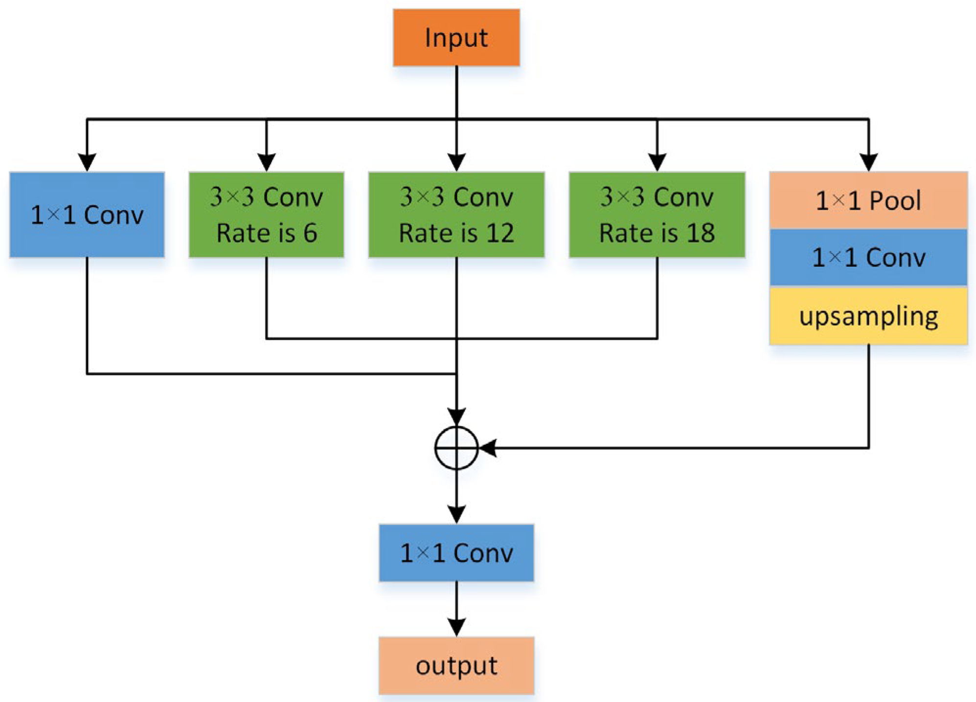
We designed a feature enhancement module (FEC) for the network construction to increase the feature representation capabilities by processing the feature maps that the backbone network retrieved in order to address the issues with the multi-scale object detection task. This module can efficiently collect objects of various scales in an input image while maintaining spatial resolution by merging data of various receptive field sizes. A global average pooling branch, three dilated convolution branches with varying expansion rates, a final fusion layer, and a 1 × 1 convolution branch make up the FEC module’s four primary components. The structure of the FEC network is shown in Figure 4. A 1 × 1 convolution kernel is used to reduce the number of channels and computational complexity, while retaining the original spatial information and alleviating the spatial information loss problem caused by multiple downsampling. Three dilated convolution branches are represented by the three distinct expansion rates (r = 6, 12, 18) that are set. These branches can expand the receptive field without increasing the number of model parameters, thereby capturing contextual information in a wider range. In this way, FEC is able to handle objects of multiple scales and improve the recognition accuracy of objects of different sizes. The global average pooling branch first applies an adaptive average pooling operation to the feature map, reducing it to a single pixel to obtain global contextual information. Then, we restore this feature map to its original size through bilinear interpolation to ensure consistency with the output of other branches. Finally, we connect the outputs of all branches along the channel dimension and further integrate the information through a 1 × 1 convolution layer to generate the final feature map. This process not only integrates the information from each branch but also plays a role in dimensionality reduction, making subsequent processing more efficient.

The feature map in the backbone network is fed into the FEC module, where it passes through the four branches mentioned above. Each branch independently extracts information of a specific type or scale. Afterwards, the results of all branches are concatenated together and processed through the fusion layer to produce an enhanced feature representation $\mathcal{F}$.

As described in Figure 1, the detection head comprises two sibling branches, which are used to carry out a dense prediction of building center points and bounding boxes. For each detected building instance, the detection box is used to identify four side center points (top, left, bottom, and right). Subsequently, these center points are regressed to obtain four extreme points (topmost, leftmost, bottommost, and rightmost) [15], which collectively define the building’s bounding box. Next, four edges are constructed: each edge is centered on one extreme point, aligned with the corresponding bounding box side, and has a length equal to 1/4 of that side. Any edge segment extending beyond the bounding box boundary is truncated. Finally, an octagonal contour is formed by sequentially connecting the endpoints of these edges [39]. The PDAA then uniformly samples vertices along this octagonal contour to generate the initial polygon.

This module efficiently generates an initial outline for each building instance. While existing contour-based methods also produce building polygons, they often incur higher inference times or yield overly smoothed shapes. In contrast, our approach eliminates the need for explicit vertex order prediction and dynamically adjusts the number of polygon vertices according to the specific building shape. This dual advantage significantly reduces inference time while simultaneously improving PolySim.

3.2. Contour Evolution Module

The initial contour obtained can only roughly represent the approximate location of the building, but it cannot accurately represent the building contour. Therefore, the vertex of the initial contour is encoded as a feature vector as the input of the contour vertex adjustment module, the offset of each point is predicted, and the offset is added to the corresponding vertex coordinate to obtain a new vertex. In order to make the building polygon concise and efficient, the redundant vertex removal module is used to remove redundant vertices and only retain the building inflection points, ensuring that the final generated polygon contains only necessary vertices, thereby improving the quality and geometric consistency of the polygon.

3.2.1. Contour Vertex Adjustment

The initial contour obtained can only roughly represent the approximate location of the building, but it cannot accurately represent the building contour. Therefore, the vertex of the initial contour is encoded as a feature vector as the input of the contour vertex adjustment module, the offset of each point is predicted, and the offset is added to the corresponding vertex coordinate to obtain the new vertex. Figure 5 shows the network structure of adjusting contour points.

Let $\widehat{\mathrm{P}}={\left\{{\widehat{\mathrm{p}}}_{\mathrm{i}}\right\}}_{\mathrm{i}=1}^{\mathrm{N}},{\widehat{\mathrm{p}}}_{\mathrm{i}}\in {\mathbb{R}}^2$ be the set of N initial points and $\widehat{\mathrm{O}}={\left\{{\widehat{\mathrm{o}}}_{\mathrm{i}}\right\}}_{\mathrm{i}=1}^{\mathrm{N}},{\widehat{\mathrm{o}}}_{\mathrm{i}}\in {\mathbb{R}}^2$ be the predicted point offset; then the prediction process is as follows:

$$\widehat{\mathrm{O}}={\mathrm{f}}_{\mathsf{\theta }}\left(\mathrm{F}\right)$$

(1)

where ${\mathrm{f}}_{\mathsf{\theta }}$ represents the vertex offset prediction mode with parameter θ. F is the input vector of the model, which is constructed as a set of feature vectors of N initial points.

$$\mathrm{F}={\left\{\mathcal{F}\left({\widehat{\mathrm{p}}}_{\mathrm{i}}\right)\circ {\widehat{\mathrm{p}}}_{\mathrm{i}}\right\}}_{\mathrm{i}=1}^{\mathrm{N}}$$

(2)

Here, $\circ$ is the concatenation operation, and ${\widehat{\mathrm{p}}}_{\mathrm{i}}$ is the coordinate of the i-th initial point. $\mathcal{F}$ is the feature map extracted by the CNN backbone, and $\mathcal{F}\left({\widehat{\mathrm{p}}}_{\mathrm{i}}\right)$ means extracting the feature vector from the feature map $\mathcal{F}$ at the coordinate ${\widehat{\mathrm{p}}}_{\mathrm{i}}$ using bilinear interpolation. The number of channels of the feature vector at position ${\widehat{\mathrm{p}}}_{\mathrm{i}}$ is the same as that of the feature map $\mathcal{F}$ (i.e., 64), and ${\widehat{\mathrm{p}}}_{\mathrm{i}}$ is a two-dimensional vector. Therefore, the input of the vertex offset prediction model is a vector of shape N × 66. The network architecture of the model is shown in Figure 5. The model consists of several standard one-dimensional convolutional layers and circular convolution (CirConv) layers [15]. The kernel sizes of circular convolution and standard one-dimensional convolution are 9 and 1, respectively.

According to the predicted vertex offset $\widehat{\mathrm{O}}$, the vertex set ${\mathrm{V}}^0$ of the initial polygon is constructed as follows:

$${\mathrm{V}}^0=\left\{{\widehat{\mathrm{p}}}_{\mathrm{i}}+{\widehat{\mathrm{o}}}_{\mathrm{i}}\mid 1\le \mathrm{i}\le \mathrm{N}\right\}$$

(3)

During training, PDAA similarly uniformly samples N target points $\mathrm{P}={\left\{{\mathrm{p}}_{\mathrm{i}}\right\}}_{\mathrm{i}=1}^{\mathrm{N}},{\mathrm{p}}_{\mathrm{i}}\in {\mathbb{R}}^2$ along the real building contours. If we let $\mathrm{Y}={\left\{{\mathrm{y}}_{\mathrm{i}}\right\}}_{\mathrm{i}=1}^{\mathrm{N}}$ be the target vertex map, then ${\mathrm{y}}_{\mathrm{i}}$ ∈$\mathrm{Y}$ is defined as

$${\mathrm{y}}_{\mathrm{i}}=\mathbb{I}\left(\exists {\mathrm{g}}_{\mathrm{j}}\in \mathrm{G}:\mathrm{i}=\mathrm{a}\mathrm{r}\mathrm{g}{ \mathrm{m}\mathrm{i}\mathrm{n}}_{\mathrm{i}}{\left\{\left|{\mathrm{p}}_{\mathrm{i}}-{\mathrm{g}}_{\mathrm{j}}\right|\right\}}_{\mathrm{i}=1}^{\mathrm{N}}\right)$$

(4)

Here, $\mathbb{I}$ is an indicator function, which takes 0 or 1. G = $\{{\mathrm{g}}_{\mathrm{j}}{\}}_{\mathrm{j}=1}^{\mathrm{M}},{\mathrm{g}}_{\mathrm{j}}\in {\mathbb{R}}^2$ represents the set of M vertices of the ground-truth building polygons. To optimize the predicted vertex graph $\widehat{\mathrm{P}}$, a focal loss [40] is applied as follows:

$${\mathcal{L}}_{\mathrm{c}\mathrm{l}\mathrm{s}}={\displaystyle \frac{-1}{{\sum }_{\mathrm{i}=1}^{\mathrm{N}}{\widehat{\mathrm{y}}}_{\mathrm{i}}}}{\sum }_{\mathrm{i}=1}^{\mathrm{N}}\left\{\begin{array}{c}{\left(1-{\widehat{\mathrm{y}}}_{\mathrm{i}}\right)}^{\mathsf{\alpha }}\mathrm{l}\mathrm{o}\mathrm{g}\left({\widehat{\mathrm{y}}}_{\mathrm{i}}\right), \mathrm{i}\mathrm{f} {\mathrm{y}}_{\mathrm{i}}=1\\ {\left(1-{\mathrm{y}}_{\mathrm{i}}\right)}^{\mathsf{\beta }}{\left({\widehat{\mathrm{y}}}_{\mathrm{i}}\right)}^{\mathsf{\alpha }}\mathrm{l}\mathrm{o}\mathrm{g}\left(1-{\widehat{\mathrm{y}}}_{\mathrm{i}}\right), \mathrm{o}\mathrm{t}\mathrm{h}\mathrm{e}\mathrm{r}\mathrm{w}\mathrm{i}\mathrm{s}\mathrm{e}\end{array}\right.$$

(5)

Here, following [41], α is set to 2 and β is set to 4. To optimize the predicted point offset, a smooth L1 loss [42] is adopted:

$${\mathcal{L}}_{\mathrm{p}\mathrm{y}}={\displaystyle \frac{1}{{\sum }_{\mathrm{i}=1}^{\mathrm{N}}{\mathsf{\omega }}_{\mathrm{i}}}}{\sum }_{\mathrm{i}=1}^{\mathrm{N}}{\mathsf{\omega }}_{\mathrm{i}}\cdot {\mathrm{s}\mathrm{m}\mathrm{o}\mathrm{o}\mathrm{t}\mathrm{h}}_{{\mathrm{L}}_1}\left({\widehat{\mathrm{p}}}_{\mathrm{i}}+{\widehat{\mathrm{o}}}_{\mathrm{i}}-{\mathrm{p}}_{\mathrm{i}}\right)$$

(6)

where ${\mathsf{\omega }}_{\mathrm{i}}={\left(0.1\right)}^{\left(1-{\mathrm{y}}_{\mathrm{i}}\right)}$ is used to scale the loss of the i-th initial point and depends on the value of ${\mathrm{y}}_{\mathrm{i}}$.

3.2.2. Redundant Vertex Removal

In the process of building vector extraction, redundant vertex removal is a key step, which aims to filter out the key vertices that best represent the building contour from the initial prediction results. As shown in Figure 6, the algorithm consists of three core modules: multi-scale feature extraction, self-attention mechanism, and learnable non-maximum suppression (NMS).

First, a multi-scale feature extractor is used to process the input data. A number of one-dimensional convolutional layers in this module are capable of capturing spatial features at various scales and offering a wealth of data for further processing. Next, a self-attention mechanism is used to enable the model to dynamically adjust the importance weight of each point according to the global context and enhance the key point recognition ability. Lastly, each point is given an importance score by a fully connected layer, and redundant points are eliminated by combining them with an enhanced non-maximum suppression algorithm.

The multi-scale feature extractor is designed to capture different scale features of the input contour. Specifically, it consists of two consecutive 1D convolutional layers, using kernels of size 3 and 5, respectively, and corresponding padding strategies to ensure that no information is lost during feature extraction. The convolution operation is followed by a batch normalization layer and a ReLU activation function to facilitate gradient flow during training. The output of the feature extractor is reshaped [B, P, 64], where B is the batch size and P is the number of vertices, to facilitate subsequent self-attention mechanism processing.

The self-attention mechanism determines the importance weight of each point by calculating the similarity score between the query, key, and value. This approach allows the model to effectively capture the relationship between points, especially in complex scenarios. The self-attention module sets the embedding dimension to 64 and uses 4-head attention to calculate the global dependencies between vertices to improve processing efficiency and flexibility.

We propose a learnable NMS predictor to more precisely eliminate redundant vertices. Using a self-attention mechanism and a multi-scale feature extractor, the predictor first evaluates the input data before creating an importance score for every point via a fully connected layer. Based on these scores, an improved NMS algorithm is applied, and the dynamic screening strategy contains two constraints: (1) Geometric constraint: if the distance between the vertex ${\mathrm{v}}_{\mathrm{i}}$ and its adjacent vertices satisfies $\mathrm{d}\left({\mathrm{v}}_{\mathrm{i}},{\mathrm{v}}_{\mathrm{i}\pm 1}\right)<{\mathsf{\tau }}_{\mathrm{d}}$. (2) Semantic constraint: if the probability ${\mathrm{s}}_{\mathrm{i}}>{\mathsf{\tau }}_{\mathrm{s}}$ is retained and the maximum confidence in the local neighborhood ${\mathcal{N}}_{\mathrm{r}}\left({\mathrm{v}}_{\mathrm{i}}\right)$ is achieved. The parameter is set to ${\mathsf{\tau }}_{\mathrm{d}}=3\mathrm{p}\mathrm{x},{\mathsf{\tau }}_{\mathrm{s}}=0.3,\mathrm{r}=3$. While considering the geometric distance, the learned importance score is also incorporated to more intelligently select which points to retain.

3.3. Missing Vertex Completion

There may be certain subtle building vertices that are not foreseen for constructing instances with more intricate geometries. To cope with this problem, PDAA proposes a missing vertex completion module, which iteratively adds new polygon vertices to the initial building polygons and matches these new polygon vertices with the unpredicted ground-truth building vertices. There are T iterations in the missing vertex recovery module. For the first iteration, the building polygons generated in the redundant vertex removal module are regarded as the initial polygons. For the t-th (2 ≤ t ≤ T) iteration, the building polygon generated by the (t − 1)-th iteration is regarded as the initial polygon. In each iteration, PDAA first uniformly samples a set of initial points along the initial polygon and then constructs a vertex and offset prediction model, as shown in Figure 7. This module takes the initial point as input to predict the vertex heatmap and point offset, where the former indicates the probability of each initial point becoming a new polygon vertex and removes redundant points, while the latter is used to refine the position of the initial point.

Formally, for the t-th iteration, let ${\widehat{\mathrm{P}}}^{\mathrm{t}}=\{{\widehat{\mathrm{p}}}_{\mathrm{i}}^{\mathrm{t}}{\}}_{\mathrm{i}=1}^{\mathrm{N}},{\widehat{\mathrm{p}}}_{\mathrm{i}}^{\mathrm{t}}\in {\mathbb{R}}^2$ be the set of N initial points uniformly sampled along the initial polygon. Then, the input features ${\mathrm{F}}^{\mathrm{t}}$ of the vertex and offset prediction model are constructed as

$${\mathrm{F}}^{\mathrm{t}}={\left\{\mathcal{F}\left({\widehat{\mathrm{p}}}_{\mathrm{i}}^{\mathrm{t}}\right)\circ {\widehat{\mathrm{p}}}_{\mathrm{i}}^{\mathrm{t}}\circ {\mathsf{\iota }}_{\mathrm{i}}^{\mathrm{t}}\right\}}_{\mathrm{i}=1}^{\mathrm{N}}$$

(7)

Here, i is the coordinate of the i-th initial point in the t-th iteration, and ${\mathsf{\iota }}_{\mathrm{i}}^{\mathrm{t}}$ takes 0 or 1, indicating whether the i-th initial point is a polygon vertex. ${\mathsf{\iota }}_{\mathrm{i}}^{\mathrm{t}}$ is defined as

$${\mathsf{\iota }}_{\mathrm{i}}^{\mathrm{t}}=\mathbb{I}\left(\exists \mathrm{v}\in {\mathrm{V}}^{\mathrm{t}-1}:\mathrm{i}=\mathrm{a}\mathrm{r}\mathrm{g}{\mathrm{m}\mathrm{i}\mathrm{n}}_{\mathrm{i}}{\left\{\left|{\widehat{\mathrm{p}}}_{\mathrm{i}}^{\mathrm{t}}-\mathrm{v}\right|\right\}}_{\mathrm{i}=1}^{\mathrm{N}}\right)$$

(8)

where ${\mathrm{V}}^{\mathrm{t}-1}$ is the vertex set of the building polygons produced at the (t − 1)-th iteration. The network architecture of this model is the same as that shown in Figure 5, except that the shape of the input vector becomes N × 67. For the t-th iteration, let ${\widehat{\mathrm{Y}}}^{\mathrm{t}}=\{{\widehat{\mathrm{y}}}_{\mathrm{i}}^{\mathrm{t}}{\}}_{\mathrm{i}=1}^{\mathrm{N}}$ and ${\widehat{\mathrm{O}}}^{\mathrm{t}}=\{{\widehat{\mathrm{o}}}_{\mathrm{i}}^{\mathrm{t}}{\}}_{\mathrm{i}=1}^{\mathrm{N}}$ be the predicted vertex map and point offsets, respectively. The vertex set ${\mathrm{V}}^{\mathrm{t}}$ of the building polygon is constructed as

$${\mathrm{V}}^{\mathrm{t}}=\left\{{\widehat{\mathrm{p}}}_{\mathrm{i}}^{\mathrm{t}}+{\widehat{\mathrm{o}}}_{\mathrm{i}}^{\mathrm{t}}\mid \left({\widehat{\mathrm{y}}}_{\mathrm{i}}^{\mathrm{t}}\ge \mathrm{s}\right)\vee \left({\mathsf{\iota }}_{\mathrm{i}}^{\mathrm{t}}=1\right),1\le \mathrm{i}\le \mathrm{N}\right\}$$

(9)

where ${\mathsf{\iota }}_{\mathrm{i}}^{\mathrm{t}}=1$ indicates that the i-th initial point is the original polygon vertex. Then, the building polygon can be generated based on ${\mathrm{V}}^{\mathrm{t}}$. Considering that each iteration may introduce new polygon vertices, which may lead to vertex redundancy, PDAA solves this problem in two steps. First, in each iteration, PDAA aims to regress redundant vertices to their adjacent ground-truth construction vertices. Second, PDAA adopts a redundant vertex removal module procedure to remove redundant vertices around building vertices [43].

3.4. Loss Function

During training, PDAA first matches the vertex set ${\mathrm{V}}^{\mathrm{t}-1}$ of the initial polygon with the vertex set G of the ground-truth building polygon. Considering the dependencies between polygon vertices, PDAA explores a variant of the dynamic time warping (DTW) algorithm [44] to implement the vertex matching process. Specifically, the DTW algorithm is first applied to match ${\mathrm{V}}^{\mathrm{t}-1}$ and G, which enables any $\begin{array}{ccc}\mathsf{\upsilon }& \in & {\mathrm{V}}^{\mathrm{t}-1}\end{array}$ to be matched with one or more consecutive vertices in ${\mathrm{G}}_{\mathrm{v}}\subseteq \mathrm{G}$, and vice versa. However, since a vertex $\begin{array}{ccc}\mathsf{\upsilon }& \in & {\mathrm{V}}^{\mathrm{t}-1}\end{array}$ can only match one ground-truth vertex in G, if $\mathrm{g}\in {\mathrm{G}}_{\mathrm{v}}$, then PDAA uniquely selects $\mathrm{g}=\mathrm{a}\mathrm{r}\mathrm{g} \mathrm{m}\mathrm{a}\mathrm{x}{\mathrm{g}}_{\mathrm{j}}{\left|\left({\mathrm{g}}_{\mathrm{j}-1}-{\mathrm{g}}_{\mathrm{j}}\right)\times \left({\mathrm{g}}_{\mathrm{j}+1}-{\mathrm{g}}_{\mathrm{j}}\right)\right|}_{{\mathrm{g}}_{\mathrm{j}}\in {\mathrm{G}}_{\mathrm{v}}}$. For brevity, the matching process is denoted as $\mathrm{V}\mathrm{D}\left(\right)$, and the ground-truth vertex that matches any $\begin{array}{ccc}\mathsf{\upsilon }& \in & {\mathrm{V}}^{\mathrm{t}-1}\end{array}$ is denoted as $\mathrm{V}\mathrm{D}\left(\mathrm{v}\right)$.

After matching the two vertex sets, PDAA samples N target points along the ground-truth building polygon. Formally, let K be the set of indices of the initial points closest to the vertex in ${\mathrm{V}}^{\mathrm{t}-1}$, $\mathrm{K}=\left\{\mathrm{a}\mathrm{r}\mathrm{g}{ \mathrm{m}\mathrm{i}\mathrm{n}}_{\mathrm{i}}\right\{\left|{\widehat{\mathrm{p}}}_{\mathrm{i}}^{\mathrm{t}}-\mathrm{v}\right|{\}}_{\mathrm{i}=1}^{\mathrm{N}}|\mathrm{v}\in {\mathrm{V}}^{\mathrm{t}-1}\}$. Then, the number of initial points between any two adjacent vertices ${\mathrm{v}}_{\mathrm{i}},{\mathrm{v}}_{\mathrm{i}+1}\in {\mathrm{V}}^{\mathrm{t}-1}$ is calculated as ${\mathrm{k}}_{\mathrm{i}+1}-{\mathrm{k}}_{\mathrm{i}}$, which is the number of target points $⟨\mathrm{V}\mathrm{D}\left({\mathrm{v}}_{\mathrm{i}}\right),\mathrm{V}\mathrm{D}\left({\mathrm{v}}_{\mathrm{i}+1}\right)⟩$ uniformly sampled along the edge. By collecting all sampled points on all edges, a set of N target points is constructed.

Let ${\mathrm{P}}^{\mathrm{t}}=\{{\mathrm{p}}_{\mathrm{i}}^{\mathrm{t}}{\}}_{\mathrm{i}=1}^{\mathrm{N}},{\mathrm{p}}_{\mathrm{i}}^{\mathrm{t}}\in {\mathbb{R}}^2$ and ${\mathrm{Y}}^{\mathrm{t}}=\{{\mathrm{y}}_{\mathrm{i}}^{\mathrm{t}}{\}}_{\mathrm{i}=1}^{\mathrm{N}}$ be the target point set and target vertex graph, respectively. Any ${\mathrm{y}}_{\mathrm{i}}^{\mathrm{t}}\in \mathrm{Y}$ is defined as

$${\mathrm{y}}_{\mathrm{i}}^{\mathrm{t}}=\mathbb{I}\left(\exists \mathrm{g}\in \mathrm{G}-\mathrm{V}\mathrm{D}\left({\mathrm{V}}^{\mathrm{t}-1}\right):\mathrm{i}=\mathrm{a}\mathrm{r}\mathrm{g}{ \mathrm{m}\mathrm{i}\mathrm{n}}_{\mathrm{i}}{\left\{\left|{\mathrm{p}}_{\mathrm{i}}^{\mathrm{t}}-\mathrm{g}\right|\right\}}_{\mathrm{i}=1}^{\mathrm{N}}\right)$$

(10)

where $\mathrm{V}\mathrm{D}\left({\mathrm{V}}^{\mathrm{t}-1}\right)\subseteq \mathrm{G}$ represents the set of ground-truth vertices matching all vertices in ${\mathrm{V}}^{\mathrm{t}-1}$. At the t-th iteration, the loss function for optimizing the predicted vertex heatmap is defined as

$$\begin{array}{ll}{\mathcal{L}}_{\mathrm{c}\mathrm{l}\mathrm{s}}^{\mathrm{t}}=& {\displaystyle \frac{-1}{{\sum }_{\mathrm{i}=1}^{\mathrm{N}}{\widehat{\mathrm{y}}}_{\mathrm{i}}^{\mathrm{t}}}}\\ & \times {\sum }_{\mathrm{i}=1}^{\mathrm{N}}\left(1-{\mathsf{\iota }}_{\mathrm{i}}^{\mathrm{t}}\right)\left\{\begin{array}{ll}{\left(1-{\widehat{\mathrm{y}}}_{\mathrm{i}}^{\mathrm{t}}\right)}^{\mathsf{\alpha }}\mathrm{l}\mathrm{o}\mathrm{g}\left({\widehat{\mathrm{y}}}_{\mathrm{i}}^{\mathrm{t}}\right)& \mathrm{i}\mathrm{f}\hspace{0.25em}{\mathrm{y}}_{\mathrm{i}}^{\mathrm{t}}=1\\ {\left(1-{\mathrm{y}}_{\mathrm{i}}^{\mathrm{t}}\right)}^{\mathsf{\beta }}{\left({\widehat{\mathrm{y}}}_{\mathrm{i}}^{\mathrm{t}}\right)}^{\mathsf{\alpha }}\mathrm{l}\mathrm{o}\mathrm{g}\left(1-{\widehat{\mathrm{y}}}_{\mathrm{i}}^{\mathrm{t}}\right)& \mathrm{o}\mathrm{t}\mathrm{h}\mathrm{e}\mathrm{r}\mathrm{w}\mathrm{i}\mathrm{s}\mathrm{e}& & \end{array}\right.\end{array}$$

(11)

Here, α and β follow the previous settings. The loss function for the offset prediction in the t-th iteration is defined as

$${\mathcal{L}}_{\mathrm{p}\mathrm{y}}^{\mathrm{t}}={\displaystyle \frac{1}{{\sum }_{\mathrm{i}=1}^{\mathrm{N}}{\mathsf{\omega }}_{\mathrm{i}}^{\mathrm{t}}}}{\sum }_{\mathrm{i}=1}^{\mathrm{N}}{\mathsf{\omega }}_{\mathrm{i}}^{\mathrm{t}}\cdot {\mathrm{s}\mathrm{m}\mathrm{o}\mathrm{o}\mathrm{t}\mathrm{h}}_{{\mathrm{L}}_1}\left({\widehat{\mathrm{p}}}_{\mathrm{i}}^{\mathrm{t}}+{\widehat{\mathrm{o}}}_{\mathrm{i}}^{\mathrm{t}}-{\mathrm{p}}_{\mathrm{i}}^{\mathrm{t}}\right)$$

(12)

where ${\mathsf{\omega }}_{\mathrm{i}}^{\mathrm{t}}={\left(0.1\right)}^{(1-\mathrm{m}\mathrm{a}\mathrm{x}\left({\mathrm{y}}_{\mathrm{i}}^{\mathrm{t}},{\mathsf{\iota }}_{\mathrm{i}}^{\mathrm{t}}\right)}$ is a scalar used to scale the loss. The overall loss function for optimizing the missing vertex recovery module is calculated as

$${\mathcal{L}}_{\mathrm{i}\mathrm{t}\mathrm{e}\mathrm{r}}={\sum }_{\mathrm{t}=1}^{\mathrm{T}}{\mathcal{L}}_{\mathrm{c}\mathrm{l}\mathrm{s}}^{\mathrm{t}}+{\mathcal{L}}_{\mathrm{p}\mathrm{y}}^{\mathrm{t}}$$

(13)

The process carried out in this study is shown in Algorithm 1.

Algorithm 1 PDAA Training

Input:  $\mathcal{X}=\{x_h{\}}_{h=1}^H$ is the set of $H$ training images; $\Pi =\{{\pi }_h{\}}_{h=1}^H$ is the set of ground-truth building polygons for $H {\mathrm{i}\mathrm{m}\mathrm{a}\mathrm{g}\mathrm{e}\mathrm{s}; }_{cer}{f}_{\mu }^{det}$ is detection model with network parameters $\mu ;f_{\nu }^{ex}$ is extreme point prediction model with network parameters $\nu ;f_{\theta }$ and $f_{{\theta }_t}^t$ are vertex and offset prediction models with network parameters $\theta$ and ${\theta }_t\left(1\le t\le T\right)$ 1: $\mathbf{for} x_h,{\pi }_h\in \mathcal{X},\Pi \mathrm{do}$ 2:    Generate ground-truth detection boxes $bb$ with ${\pi }_h$ 3:    Extract Feature map and predict detection boxes: $\mathcal{F},\widehat{b}b\leftarrow f_{\mu }^{det}\left(x_h\right)$ 4:    $\mathrm{P}\mathrm{r}\mathrm{e}\mathrm{d}\mathrm{i}\mathrm{c}\mathrm{t} \mathrm{e}\mathrm{x}\mathrm{t}\mathrm{r}\mathrm{e}\mathrm{m}\mathrm{e} \mathrm{p}\mathrm{o}\mathrm{i}\mathrm{n}\mathrm{t}\mathrm{s}:\widehat{ex}\leftarrow f_{\nu }^{ex}\left(\mathcal{F},bb\right)$, and generate target $ex$ 5:    Sample initial points $\widehat{P}$ along contour formed by $\widehat{ex}$ 6:    Construct input vector $F$ with $\mathcal{F}$ and $\widehat{P}($ Equation (2)) 7:    $\widehat{O},\widehat{Y}\leftarrow f_{\theta }\left(\tilde{F}\right)$ 8:    Generate targets $P$ and $Y$ with ${\pi }_h$ (Equation (4)) 9:   $\mathbf{for} t=1$ to $T \mathbf{do}$ 10:      Compute vertex set $V^{t-1}$ from $\{\widehat{O},\widehat{Y}\}\left(t=1,\mathrm{E}\mathrm{q}\mathrm{u}\mathrm{a}\mathrm{t}\mathrm{i}\mathrm{o}\mathrm{n}\left(3\right)\right)$     or ${\left\{{\widehat{\widehat{O}}}^{t-1},{\widehat{Y}}^{t-1}\right\}}_{\widehat{A}}(t>1$, Equation (9)) 11:       Sample points ${\widehat{P}}^t$ along polygon formed by $V^{t-1}$ 12:      Construct input vector $F^t$ with $\mathcal{F}$ and ${\widehat{P}}^t($ Equation (7)) 13:      ${\widehat{O}}^t,{\widehat{Y}}^t\leftarrow {\widehat{f}}_{{\theta }_t}^{\dot{t}}\left(F^t\right)$ 14:       Generate targets $P^{\iota }$ and $Y^{\iota }$ with ${\pi }_h$ and ${\widehat{P}}^{\iota }$(Equation (10)) 15:    end for 16:    $\mathrm{C}\mathrm{o}\mathrm{m}\mathrm{p}\mathrm{u}\mathrm{t}\mathrm{e} \mathrm{L}\mathrm{o}\mathrm{s}\mathrm{s}\mathrm{e}\mathrm{s} {\mathcal{L}}_{det} and {\mathcal{L}}_{ex} with \widehat{bb},bb,\widehat{e}x,ex$ 17:    $\mathrm{C}\mathrm{o}\mathrm{m}\mathrm{p}\mathrm{u}\mathrm{t}\mathrm{e} \mathrm{L}\mathrm{o}\mathrm{s}\mathrm{s}\mathrm{e}\mathrm{s} {\mathcal{L}}_{cls}, {\mathcal{L}}_{py}, and {\mathcal{L}}_{iter} \mathrm{w}\mathrm{i}\mathrm{t}\mathrm{h} \widehat{O}, \widehat{P}, \widehat{Y}, P$      $Y$, ${\tilde{O}}^t$, ${\widehat{P}}^t$, ${\widehat{Y}}^t$,$P^t$, $Y^t(\mathrm{E}\mathrm{q}\mathrm{u}\mathrm{a}\mathrm{t}\mathrm{i}\mathrm{o}\mathrm{n}\mathrm{s}$ (5), (6) and (13)) 18:    $\mathcal{L}\leftarrow {\mathcal{L}}_{det}+{\mathcal{L}}_{ex}+{\mathcal{L}}_{cls}+{\mathcal{L}}_{py}+{\mathcal{L}}_{iter}$ 19:    $\mathrm{U}\mathrm{p}\mathrm{d}\mathrm{a}\mathrm{t}\mathrm{e} \mu ,\nu ,\theta , \mathrm{a}\mathrm{n}\mathrm{d} {\theta }_t \mathrm{by} \mathrm{backpropagating} \mathrm{loss}\mathcal{L}$ 20:$\mathbf{end} \mathbf{for}$

4. Experiment

In all experiments, the models were trained for 150 epochs on an NVIDIA GTX 1080 Ti GPU using a mini-batch size of eight images. The initial learning rate of the Adam optimizer was 1 × 10⁻⁴. The learning rate was halved at 80 and 120 epochs. The models were trained with multi-scale data augmentation and tested without tricks. The CNN backbone was initialized with weights pre-trained on ImageNet, while the other layers were initialized as in [15].

4.1. Datasets and Evaluation Metrics

We evaluated our proposed method on three building datasets: the WHU dataset [45], the Vaihingen dataset [46], and the Inria building dataset [47]. The WHU dataset has a large number of highly accurate building labels. The dataset covers an area of 450 square kilometers and includes more than 187,000 buildings of various architectures and uses. All aerial images are seamlessly cropped into 1024 × 1024 blocks. Following [8], the original images with a resolution of 0.075 m/pixel are downsampled to 0.2 m/pixel, and 130,000/14,500/42,000 buildings are used for training/validation/testing datasets, respectively. The Vaihingen dataset covers the area of Vaihingen, a small town near Stuttgart, Germany, and provides high-resolution (9 cm/pixel) aerial images, consisting of 168 images of size 512 × 512 and a resolution of 0.09 m/pixel. Following [10], the dataset is split into 100/68 images for training/testing. The Inria building dataset contains 360 images of size 5000 × 5000 pixels and a resolution of 0.3 m/pixel collected from five different cities (Austin, Chicago, Kitsap, Tyrol, and Vienna). To adapt to specific experimental requirements, these original images are first padded to 5120 × 5120 pixels and then cropped into small patches of 512 × 512 pixels. Following [14], the city of Tyrol is selected from the Inria dataset to evaluate the proposed algorithm. In the experiment, it is divided into training and test sets in a ratio of 3:1.

To evaluate the performance of methods for generating building polygons, classic metrics in the field of object detection and instance segmentation are used: AP (averaged over intersection-over-union (IoU) thresholds of 0.50:0.05:0.95), AP₅₀ (IoU threshold of 0.5), and AP₇₅ (IoU threshold of 0.75). AP_S emphasizes the importance of accurate and complete detection of building instances and is widely used in existing methods [13,15,24]. Unless otherwise specified, IoU in AP_S is based on building polygons rather than detection boxes. In addition, to evaluate the geometric similarity between the polygons generated by different methods and the ground-truth building polygons, we also evaluated the PolySim metric, as used in previous studies [10,48]. Specifically, PolySim is calculated as the product of the average difference in the orientation angles of all edges of two polygons and the IoU value between the two polygons.

$$\mathrm{P}\mathrm{o}\mathrm{L}\mathrm{i}\mathrm{S}\left(\mathrm{X},\mathrm{Y}\right)={\displaystyle \frac{1}{2 \mathrm{m}}}{\sum }_{{\mathrm{x}}_{\mathrm{i}}\in \mathrm{X}}{\mathrm{m}\mathrm{i}\mathrm{n}}_{\mathrm{y}\in \partial \mathrm{Y}}\parallel {\mathrm{x}}_{\mathrm{j}}-\mathrm{y}\parallel +{\displaystyle \frac{1}{2 \mathrm{n}}}{\sum }_{{\mathrm{y}}_{\mathrm{j}}\in \mathrm{Y}}{\mathrm{m}\mathrm{i}\mathrm{n}}_{\mathrm{x}\in \partial \mathrm{X}}\parallel {\mathrm{y}}_{\mathrm{j}}-\mathrm{x}\parallel$$

(14)

Here, the first term is the average distance between each vertex ${\mathrm{x}}_{\mathrm{i}}\in \mathrm{X}$, $\mathrm{i}$= 1, …, m and its closest point $\mathrm{y}$ on the polygon’s boundary, while the second term is the average distance between each vertex ${\mathrm{y}}_{\mathrm{j}}\in \mathrm{Y},\mathrm{j}=1,\dots ,\mathrm{n}$ and its closest point on the polygon’s boundary to the point $\mathrm{x}$.

In addition, to evaluate the efficiency of different methods, the inference time (Time) and the number of learnable parameters (Params) were calculated.

4.2. Results and Analysis

We compare our proposed algorithm with the pixel-based method Mask R-CNN [24], as well as recent contour-based methods including MA-FCN [11], Polygon-RNN++ [15], APGA [12], Deep Snake [17], and Hisup [12]. For a fair comparison, the detection boxes generated by PDAA are fed to Polygon-RNN++ and APGA at inference time.

4.2.1. Results from WHU Dataset

Table 1. Comparison of different methods on the WHU dataset.

Method	AP	AP50	AP75	PolySim	Parama (M)	Time (ms)
Mask R-CNN	0.707	0.904	0.803	0.820	63.62	103.77
MA-FCN	0.674	0.858	0.764	0.821	22.48	41.90
Polygon-RNN++	0.701	0.908	0.796	0.812	58.00	1431.03
APGA	0.708	0.905	0.794	0.821	52.43	345.92
Deep Snake	0.736	0.911	0.823	0.844	23.11	46.36
HiSup	0.735	0.864	0.798	0.846	74.29	99.21
PDAA	0.754	0.912	0.835	0.849	25.55	40.69

shows the numerical results of the different methods used on the WHU dataset. As a typical representative of semantic segmentation, MA-FCN focuses on distinguishing between buildings and non-building areas without involving the identification of specific building instances. This mechanism minimizes the amount of learnable parameters required by MA-FCN and also significantly reduces the inference time. However, this advantage also brings limitations, especially when dealing with densely distributed building instances; for example, MA-FCN has difficulty in effectively distinguishing adjacent buildings, resulting in its performance on the WHU dataset being lower than expected. Similarly, HiSup generates polygons by relying on the results of semantic segmentation, which helps improve the overall segmentation quality, but may also cause the generated polygon shapes to deviate from the ground truth of the actual building. In addition, HiSup can simultaneously learn mask, line, and vertex information to improve segmentation results, but this also means that it requires more learnable parameters and longer reasoning time than MA-FCN. In contrast, methods that distinguish different instances: Mask R-CNN, Polygonrnn++, APGA, and Deep Snake show significant improvements in average precision (AP_S) and polygon similarity (Polysim).

In the WHU dataset, PDAA shows significant performance advantages, not only surpassing existing methods by more than 2% in AP but also achieving up to a 6% performance improvement in core evaluation indicators such as AP, AP₅₀, and AP₇₅. This is a considerable improvement for methods that have already achieved good results on the WHU dataset. The results of the WHU dataset are visualized in Figure 8. MA-FCN faces particular challenges when dealing with adjacent building instances, and its use of the empirical regularization algorithm can cause the generated building contour to deviate from the target, producing inaccurate boundary predictions. Polygonrnn++ misses several vertices in the process of generating buildings, producing incorrect building contours in building instances with complex shapes. Although APGA can generate relatively regular building shapes, their contours do not necessarily strictly fit the target building boundaries. HiSup faces great challenges in distinguishing adjacent building instances, which may lead to errors in building prediction. Instead, PDAA performs better in both building instance recognition and accurate boundary prediction. The generated building polygons contain only necessary vertices, presenting a structure that is more consistent with the ground truth and making the prediction results closer to the geometric characteristics of real buildings, thereby improving the quality and geometric consistency of polygons.

4.2.2. Results from Vaihingen Dataset and Inria Dataset

As shown in

Table 2. Comparison of different methods on the Vaihingen dataset.

Method	AP	AP50	AP75	PolySim
Mask R-CNN	0.565	0.771	0.649	0.789
MA-FCN	0.497	0.697	0.563	0.726
Polygon-RNN++	0.513	0.740	0.592	0.749
APGA	0.570	0.780	0.659	0.793
Deep Snake	0.585	0.752	0.662	0.813
HiSup	0.609	0.784	0.682	0.819
IPDD	0.621	0.801	0.732	0.813

, this study conducted a multi-method comparison experiment on the Vaihingen dataset. The experiment shows that the performance of the Polygon-RNN++ method is significantly lower than that of other methods using contour information. This phenomenon is mainly attributed to the limitations of Polygon-RNN++ in processing fine structures in high-spatial-resolution images. In contrast, PDAA demonstrates its superiority, especially in more accurate predictions, producing simpler building contours and reducing the generation of redundant points. Compared with HiSup, PDAA not only achieves a similar performance level in PolySim indicators, but it also achieves a more than 2% improvement in AP, AP₅₀, and AP₇₅ accuracy standards, which highlights the advantage of PDAA in achieving higher accuracy predictions. To more intuitively demonstrate these results, some visualization examples in the Vaihingen dataset are presented in Figure 9.

The numerical results on the Inria dataset are reported in

Table 3. Comparison of different methods on the Inria dataset.

Method	AP	AP50	AP75	PolySim
Mask R-CNN	0.391	0.687	0.411	0.638
MA-FCN	0.364	0.622	0.379	0.642
Polygon-RNN++	0.415	0.707	0.438	0.639
APGA	0.410	0.682	0.439	0.637
Deep Snake	0.429	0.712	0.460	0.699
HiSup	0.458	0.711	0.513	0.686
IPDD	0.465	0.714	0.518	0.690

. PDAA performs better than APGA in terms of AP, AP₇₅, and PolySim, with an improvement of more than 6%, respectively. At the same time, PDAA also shows strong competitiveness in the AP₅₀ indicator. Compared with other methods, PDAA’s significant improvements in AP and AP₇₅ further demonstrate PDAA’s excellent ability in accurately depicting building contours.

Whether for the detailed Vaihingen dataset or the larger Inria dataset, PDAA shows obvious advantages over other existing methods, especially in improving the accuracy of building contour prediction. The accuracy and effect of these methods are significantly different from those of the WHU dataset. This is because the large number of small auxiliary structures in the Vaihingen scene puts higher requirements on local feature extraction, while the diversity of architectural styles in the Inria dataset tests the generalization representation ability of the model.

4.3. Ablation Experiment

In order to more deeply and comprehensively evaluate the effectiveness of each key module in the PDAA framework, a series of ablation experiments were conducted to carefully analyze the impact of each component on the final performance. All experiments were conducted on the WHU dataset, and it was ensured that they were performed in the same experimental environment. The training parameters (such as learning rate, batch size, etc.) were kept consistent to ensure that the experimental results were highly comparable and reliable.

Table 4. Ablation study of the proposed algorithm. The marked items in the table indicate the addition of this module.

Baseline	RVRM	MVCM	FEC	WHU Dataset
				AP	AP50	AP75	PolySim
√				0.744	0.901	0.825	0.835
√	√			0.745	0.903	0.828	0.839
√	√	√		0.747	0.904	0.827	0.848
√	√	√	√	0.754	0.912	0.835	0.849

shows, in detail, the performance changes under different module combinations. Among them, the introduction of the FEC module significantly improves the performance of the model, which shows that FEC plays a vital role in optimizing feature extraction. In addition, the addition of the missing vertex completion module (MVCM) further improves the PolySim score to 84.8%, showing its great potential in improving contour shape accuracy. In particular, when the redundant vertex removal module (RVRM), the missing vertex completion module, and the FEC are used together, the AP value reaches 75.4%. This result not only reflects the importance of each of the three modules but also reveals the synergistic effect between them, especially the outstanding performance in dealing with complex building structure extraction tasks.

Figure 10 intuitively shows the changing process of the building extraction effect under different module combinations. It can be clearly seen from the figure that without the application of RVRM, MVCM, and FEC, the predicted building contour has obvious vertex deviation, inaccurate positioning, and a loss of important vertices (Figure 10b). With the gradual introduction of RVRM, it can be seen that the prediction of redundant point vertices has been effectively controlled (Figure 10c), while MVCM has successfully restored some missing key point vertices (Figure 10d). Although the overall prediction of the building contour is now quite close to the actual situation, there are still certain errors in the positions of some vertices. Finally, by adding the FEC module, these subtle deviations have been effectively corrected, achieving a more accurate building contour prediction (Figure 10e).

To further emphasize the importance of each module and the interaction mechanism between them, we also analyzed the specific reasons for the improvement at each stage. RVRM reduces unnecessary calculations and potential sources of error by identifying and removing redundant points; MVCM uses multi-angle information to make up for missing information, thereby improving reconstruction accuracy; and the FEC module enhances feature expression capabilities, allowing the model to more accurately capture the detailed features of the building. This multi-level, all-round optimization strategy works together to enable the PDAA framework to demonstrate excellent performance in building extraction tasks.

4.4. Discussion

The end-to-end polygon dynamic adjustment algorithm (PDAA) proposed in this study has shown significant performance advantages in the task of building contour extraction. The core of this method is to solve many key challenges of traditional methods through the synergy of four modules. First, the local feature extraction strategy focusing on the region of interest (RoI) effectively reduces the redundancy of global features, allowing the model to more accurately capture the local geometric details of the building. This design is inspired by the sensitivity of the human visual system to local features. By positioning the RoI detection box, the model’s adaptability to complex building structures is significantly improved.

Secondly, the feature enhancement module, FEC, significantly enhances the model’s ability to detect key vertices in complex backgrounds by optimizing feature expression capabilities. The introduction of this module compensates for the sensitivity of traditional vertex detection methods to illumination changes and texture interference. FEC reduces the risk of missing vertices by enhancing the robustness of features. In the ablation experiment, the introduction of FEC improved the accuracy of the model in complex building examples by about 1%, which shows that its enhancement effect on key features cannot be ignored.

The synergy between the redundant vertex removal module and the missing vertex completion module is one of the core innovations of PDAA. Traditional methods often lead to the accumulation of redundant vertices or the loss of key vertices due to the lack of a dynamic adjustment mechanism. The redundant vertex removal module effectively distinguishes redundant points from key points through a learnable classification mechanism, significantly reducing the number of redundant vertices of polygons (as shown in Figure 8). At the same time, the missing vertex completion module restores vertices missed due to occlusion or noise interference through iterative optimization. This dynamic adjustment mechanism not only improves the geometric consistency of polygons but also avoids the shape distortion problem caused by a fixed number of vertices. In the experiment, the combined use of the redundant vertex removal module and the missing vertex completion module increased the PolySim score to 84.8%, proving its effectiveness in complex contour modeling.

This study conducted experiments on the WHU, Vaihingen, and Inria datasets, and the results showed significant performance differences among the datasets. The WHU dataset, due to its high-quality annotations and simple building forms, allows PDAA to fully utilize the advantages of its vertex adjustment mechanism and obtain higher scores. In contrast, the Vaihingen and Inria datasets contain more complex building forms and inconsistent annotations, which leads to a decrease in the performance of PDAA. These differences reveal the challenges faced by PDAA in dealing with complex building outlines and provide guidance for further optimization.

However, this study still has some limitations. PDAA’s reliance on RoI detection boxes may lead to a decline in its performance in dense building complexes. When the detection boxes overlap or have positioning deviations, it may affect the accuracy of subsequent vertex predictions. In addition, the current method’s reliance on high-quality labeled data still needs to be further reduced. In future studies, the model’s feature extraction capabilities for overlapping areas or fuzzy boundaries can be enhanced by introducing a multi-scale attention module, and the deviations of local RoI detection boxes can be corrected using global context information to improve the global consistency of vertex predictions. Semi-supervised or self-supervised learning strategies can be introduced to reduce the cost of manual labeling. Pseudo-annotations are dynamically generated during training, and consistency regularization constraints are added to improve the model’s generalization ability for unseen data.

It is worth mentioning that the good geometric consistency shown by PDAA not only reflects its effectiveness in building extraction tasks but also provides a solid foundation for practical applications. This method can be widely used in scenarios such as urban planning, disaster assessment, and the automatic interpretation of remote sensing images. The building polygons extracted by PDAA can be used as high-quality vector inputs: after natural disasters, the rapid extraction of damaged building outlines is helpful for loss assessment and reconstruction planning; accurate building boundary information can assist in the construction of high-precision maps and improve environmental perception capabilities. These potential application directions also further highlight the research value and promotional significance of the PDAA method.

5. Conclusions

In this paper, an end-to-end polygon dynamic adjustment algorithm (PDAA) is proposed to solve the challenge of extracting building contours in remote sensing images. By focusing on the collaborative optimization of modules such as the local feature extraction of RoI, redundant contour removal, and missing contour completion, PDAA has achieved significant improvements in the geometric similarity and extraction accuracy of complex building contours. Experiments show that PDAA achieves 75.4% AP and 84.8% PolySim scores on the WHU dataset, verifying its effectiveness in processing redundant vertices, recovering missing vertices, and adapting to changing building forms. Compared with existing methods, PDAA simplifies the prediction process, reduces dependence on large-scale annotated data, and generates polygons that are closer to real geometric features through a dynamic adjustment mechanism. The main contributions of this study include the following: (1) proposing an RoI local feature extraction strategy, which significantly improves the adaptability of complex buildings; (2) designing redundant point removal and missing point completion modules, which solves the shape distortion problem caused by the fixed number of vertices in traditional methods; and (3) through module design, efficient and high-precision end-to-end prediction is achieved, providing reliable technical support for practical engineering applications. Future work should focus on a lightweight optimization of the algorithm and improvement in cross-domain generalization capabilities to further promote the practical application of remote sensing image analysis technology.