DFAST: A Differential-Frequency Attention-Based Band Selection Transformer for Hyperspectral Image Classification

Abstract

Hyperspectral image (HSI) classification faces challenges such as high dimensionality, spectral redundancy, and difficulty in modeling the coupling between spectral and spatial features. Existing methods fail to fully exploit first-order derivatives and frequency domain information, which limits classification performance. To address these issues, this paper proposes a Differential-Frequency Attention-based Band Selection Transformer (DFAST) for HSI classification. Specifically, a Differential-Frequency Attention-based Band Selection Embedding Module (DFASEmbeddings) is designed to extract original spectral, first-order derivative, and frequency domain features via a multi-branch structure. Learnable band selection attention weights are introduced to adaptively select important bands, capture critical spectral information, and significantly reduce redundancy. A 3D convolution and a spectral–spatial attention mechanism are applied to perform fine-grained modeling of spectral and spatial features, further enhancing the global dependency capture of spectral–spatial features. The embedded features are then input into a cascaded Transformer encoder (SCEncoder) for deep modeling of spectral–spatial coupling characteristics to achieve classification. Additionally, learnable attention weights for band selection are outputted for dimensionality reduction. Experiments on several public hyperspectral datasets demonstrate that the proposed method outperforms existing CNN and Transformer-based approaches in classification performance.

1. Introduction

Hyperspectral imaging technology, as an important component of the unmanned aerial vehicle remote sensing and satellite remote sensing field, captures continuous spectral information across visible to near-infrared wavelengths, providing abundant spectral and spatial features for target recognition and analysis [1,2]. In recent years, hyperspectral imaging has demonstrated significant application potential in fields such as agricultural monitoring, urban planning, environmental monitoring, and disaster management [3,4]. Compared with traditional RGB and multispectral images, hyperspectral images offer higher spectral resolution and a broader range of wavelengths, enabling more accurate representation of surface object characteristics. However, the high dimensionality, spectral redundancy, and complex coupling of spectral–spatial features in hyperspectral images pose significant challenges for classification and data analysis [5].

In the early stages of hyperspectral image classification, traditional methods primarily relied on hand-crafted feature extraction techniques, such as support vector machines (SVM) [6], random forests (RF) [7], k-nearest neighbor (k-NN) [8], and principal component analysis (PCA) [9]. While these methods achieved satisfactory performance in certain specific scenarios, they were limited by their reliance on manually designed features and failed to fully capture the deep information inherent in hyperspectral data. This limitation is particularly evident when dealing with complex nonlinear data structures [10].

In recent years, deep learning techniques have become the mainstream research direction for hyperspectral image classification. The introduction of convolutional neural networks (CNNs) and vision transformers (ViTs) has achieved remarkable progress in this field [11]. Chen et al. [12] proposed a hyperspectral classification method based on 1D CNNs, which directly extracts features from the spectral domain. Lee and Kwon [13] designed a context-aware 2D CNN to capture the spatial information in hyperspectral images. Zhong et al. [14] developed a 3D CNN model that jointly utilizes spectral and spatial information for classification. These methods effectively extract spectral and spatial features in hyperspectral images through the local connectivity and weight-sharing mechanisms of CNNs. However, due to the limited receptive field of convolution operations, CNNs struggle to capture long-range global dependencies, making it difficult to model long-range feature interactions in hyperspectral data [15].

To address this limitation, the Residual Network (ResNet) introduces residual connections to mitigate the vanishing gradient problem, making it easier to train deeper networks [16]. Moreover, recent research has incorporated attention mechanisms and Transformers into hyperspectral classification, providing new solutions for capturing global features and long-range dependencies. For instance, Sun et al. [17] proposed the Spectral–Spatial Feature Token Transformer (SSFTT), which combines a spectral–spatial feature extraction module and a Transformer encoder to capture spectral–spatial and semantic features in hyperspectral data. Yang et al. [18] introduced the Hyperspectral Image Transformer (HiT), embedding convolution operations into the Transformer to capture subtle spectral differences and propagate local spatial context information. Hong et al. [19] developed SpectralFormer, which achieves efficient hyperspectral data classification through intra-group spectral embedding and inter-layer fusion. These Transformer-based methods overcome CNN’s limitations in global dependency modeling but still face challenges in addressing spectral redundancy and capturing complex spectral–spatial coupling characteristics.

In addition to traditional CNN and Transformer models, innovative hybrid network architectures have emerged in recent years. For example, Roy et al. [20] proposed the morphFormer model, which incorporates spectral and spatial morphological convolution modules with a Transformer encoder to effectively capture the spectral–spatial features of hyperspectral images and enhance classification performance. MorphFormer leverages morphological operations to extract the geometric shapes and structural characteristics of objects, while the multi-head attention mechanism strengthens the interaction between spectral and spatial features, providing strong support for further optimizing hyperspectral classification tasks.

To address the spectral redundancy challenges in HSI classification, researchers have developed various dimensionality reduction approaches, which are primarily categorized into feature extraction (FE) and feature selection (FS) [21]. Feature extraction methods project high-dimensional hyperspectral data into a lower-dimensional space through transformations such as PCA or manifold learning [22], while feature selection (also termed band selection) preserves the original physical meaning of spectral bands by selecting the most informative subsets [23]. Band selection can be further classified into supervised and unsupervised methods depending on whether labeled data is utilized [24,25]. In practice, due to the difficulty of acquiring sufficient labeled samples [26], unsupervised band selection has become a more practical and widely studied solution.

Existing band selection techniques mainly fall into three types: ranking-based [27,28], clustering-based [29], and searching-based [30,31]. Among these, clustering-based methods have demonstrated particular effectiveness by grouping spectrally similar bands and selecting representative ones. These can be subdivided into density clustering [32], hierarchical clustering [33], graph clustering [34], and partition clustering [35]. Notably, partition clustering—which groups highly correlated bands while separating dissimilar ones—has shown superior performance for HSI. Wang et al. [36] further proposed the continuous band indexes constraint (CBIC) for ordered partition clustering, explicitly considering the strong correlation between adjacent bands in hyperspectral imagery. These studies provide critical theoretical and methodological foundations for developing adaptive band selection mechanisms to reduce spectral redundancy while preserving discriminative features.

Compared with traditional methods, the proposed DFAST in this paper achieves more discriminative feature representation while avoiding information loss common in feature extraction approaches, through the fusion of multi-branch spectral derivatives and frequency domain features. Existing band selection methods primarily fall into three categories: ranking-based, clustering-based, and search-based approaches. While typical clustering methods such as partition clustering require predefined cluster numbers and are prone to local optima, our learnable band selection attention mechanism overcomes these limitations through dynamic weight adjustment. Although the CBIC method proposed by Wang et al. inspired our spectral–spatial coupling design, its manually designed constraints lack the adaptive fusion capability based on attention mechanisms.

Despite the significant progress made by existing methods in hyperspectral image classification tasks, they still exhibit limitations in handling spectral redundancy, capturing first-order spectral derivative information, and modeling the global dependencies of spectral–spatial features. Furthermore, the presence of extensive redundant bands in hyperspectral data can significantly affect the efficiency and classification performance of models. Therefore, developing an effective band selection mechanism to reduce spectral redundancy while preserving critical spectral information remains an urgent issue to address.

To address the aforementioned challenges, this paper proposes DFAST for hyperspectral image classification. The DFASEmbeddings utilizes a multi-branch structure to extract original spectral features, first-order derivatives, and frequency domain features. Learnable band selection attention weights are introduced to adaptively select important bands, capture critical spectral information, and significantly reduce redundancy. Furthermore, 3D convolution and a spectral–spatial attention mechanism are employed for fine-grained modeling of spectral and spatial features, enhancing the global dependency capture of spectral–spatial features.

To achieve deep feature fusion, this paper proposes SCEncoder. By stacking multiple Transformer modules, SCEncoder captures the global coupling relationships between spectral and spatial features, while residual connections alleviate the vanishing gradient problem and ensure stable training [37]. Additionally, the model introduces a learnable class token, which efficiently aggregates spectral and spatial features and completes the hyperspectral classification task through the classification head. Moreover, the learnable band selection attention weights output by the model can be used for dimensionality reduction of hyperspectral images, effectively reducing the signal-to-noise ratio (SNR) of spectral channels.

The main contributions of this paper are as follows:

• DFASEmbeddings is proposed, which extracts discriminative features from original spectral data, first-order derivatives, and frequency domain features. This module reduces spectral redundancy and optimizes band selection while enhancing spatial dependencies through fine-grained modeling of spectral and spatial features using 3D convolution, thereby achieving effective spectral feature embedding.
• Learnable band selection weights are introduced to adaptively select important spectral bands, improving classification performance while simultaneously outputting band selection weights. These weights can be used to reduce the dimensionality of hyperspectral data, effectively decreasing the number of network parameters, reducing training time, and improving classification accuracy.
• SCEncoder is proposed to capture the global coupling relationships between spectral and spatial features through a deep network, while residual connections ensure the stability of training in deep networks.

Experiments conducted on several public hyperspectral datasets demonstrate that the proposed method outperforms existing CNN- and Transformer-based approaches in terms of classification performance. The proposed method effectively addresses issues such as spectral redundancy, spatial dependency, and limited training samples.

2. Related Work

2.1. HSIChannelAttention Module

The spectral dimension of HSI is typically very high, often comprising tens to hundreds of channels. However, not all channels significantly contribute to the target task. To address this, the HSIChannelAttention module introduces a channel attention mechanism [38], as illustrated in Figure 1, to assign weights to each channel. This mechanism automatically selects the spectral channels that are relevant to the task while suppressing noise information. By computing optimal channel selection weights, the output feature tensor becomes more focused on critical information, enhancing the overall feature representation.

Assume that the input hyperspectral feature tensor is denoted as $F\in R^{C\times H\times W}$, where C represents the number of spectral channels, and H and W denote the height and width of the feature map, respectively. The goal is to generate a channel selection weight vector $W_c\in R^C$ and apply it to each channel of the input feature tensor.

Firstly, maximum pooling and average pooling operations are performed on each channel along the spatial dimensions to obtain two channel feature vectors, $F_{\max }$ and $F_{\mathrm{avg}}$, respectively. The formulas are as follows:

$$F_{\max }=\mathrm{MaxChannelPool}\left(F\right),F_{\mathrm{avg}}=\mathrm{AvgChannelPool}\left(F\right)$$

(1)

Here, maximum pooling extracts the maximum value features from each channel, while average pooling extracts the average value features from each channel. These two methods preserve global information from different perspectives.

Next, the two channel feature vectors are input into a shared one-dimensional convolutional layer, Conv1D, to extract higher-level feature representations:

$$F_{\mathit{max}}^{’}=\mathit{Conv}1D\left(F_{\mathit{max}}\right), F_{\mathit{avg}}^{’}=\mathit{Conv}1D\left(F_{\mathit{avg}}\right)$$

(2)

The shared convolution operation ensures consistency in the feature extraction process across the two paths.

Subsequently, the intermediate feature representations from the two paths are fused by element-wise addition to calculate the fused feature $F_{\mathrm{merge}}$:

$$F_{\mathit{merge}}=F_{\mathit{max}}^{’}+F_{\mathit{avg}}^{’}$$

(3)

The fused feature is then passed through a Sigmoid(S) activation function to compute the channel selection weight $W_c$:

$$W_c=S\left(F_{\mathit{merge}}\right)$$

(4)

The Sigmoid function normalizes the weight values to the range [0, 1], where the weight of each channel represents its importance.

Finally, the channel selection weight $W_c$ is applied element-wise to each channel of the input feature tensor F, generating the weighted output feature $F_c$:

$$F_c=F\odot W_c$$

(5)

Here, ⊙ denotes element-wise multiplication along the channel dimension.

Through this channel attention mechanism, the HSIChannelAttention module can automatically suppress the influence of irrelevant channels and highlight the features of critical spectral channels, effectively enhancing the modeling capability of hyperspectral data.

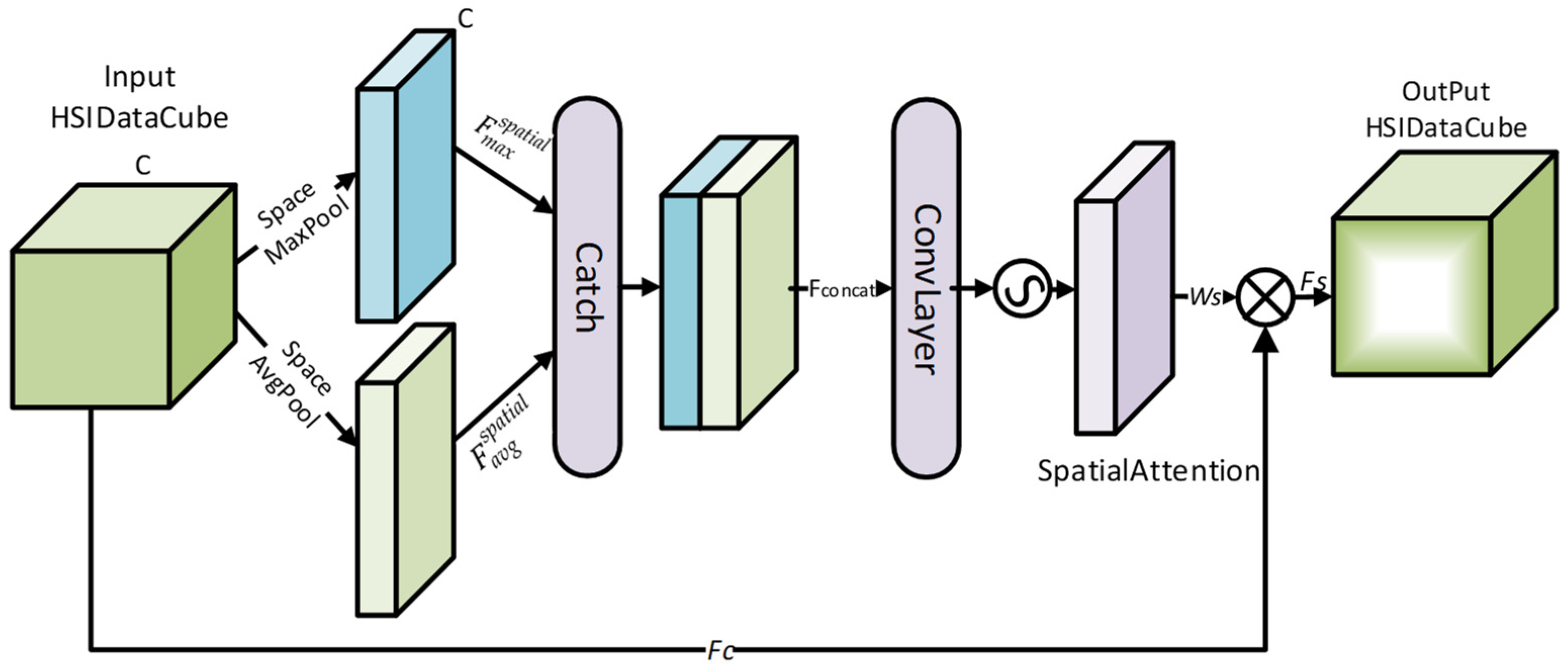
2.2. HSISpatialAttention Module

In hyperspectral images, it is essential to consider not only spectral information but also pixel correlations in the spatial dimensions. Pixels of the same class often exhibit strong spatial aggregation. Therefore, the HSISpatialAttention module introduces a spatial attention mechanism [38], as shown in Figure 2, to dynamically adjust the positional weights of each pixel and optimize the feature representation for classification.

Assume that the channel attention-weighted feature tensor is denoted as $F_c\in R^{C\times H\times W}$. First, maximum pooling and average pooling are applied along the spectral dimension C to extract spatial features:

$$F_{\mathit{max}}^{\mathit{spatial}}=\mathit{MaxSpatialPool}\left(F_c\right), F_{\mathit{avg}}^{\mathit{spatial}}=\mathit{AvgSpatialPool}\left(F_c\right)$$

(6)

Maximum pooling retains the maximum feature value at each pixel position across all channels, while average pooling retains global average information at each pixel position. This allows the capture of both significant local and global features.

Next, the two feature maps are concatenated along the channel dimension to form the fused feature $F_{\mathrm{concat}}$:

$$F_{\mathit{concat}}=\mathit{Concat}\left(F_{\mathit{max}}^{\mathit{spatial}},F_{\mathit{avg}}^{\mathit{spatial}}\right)$$

(7)

The fused feature map is then passed through a 2D convolution operation to generate the spatial weight matrix $W_s$:

$$W_s=\sigma \left(\mathit{Conv}2D(F_{\mathit{concat}})\right)$$

(8)

The 2D convolution extracts local patterns in the spatial dimensions and produces a weight matrix $W_s$ that reflects the importance of each pixel.

Finally, the spatial weight matrix $W_s$ is applied element-wise to all channels of the feature tensor $F_c$, resulting in the weighted output feature $F_s$:

$$F_s=F_c\odot W_s$$

(9)

This process dynamically enhances the feature extraction capability for key regions while effectively suppressing the interference of background noise. As a result, the final feature representation becomes more precise in the spatial dimensions.

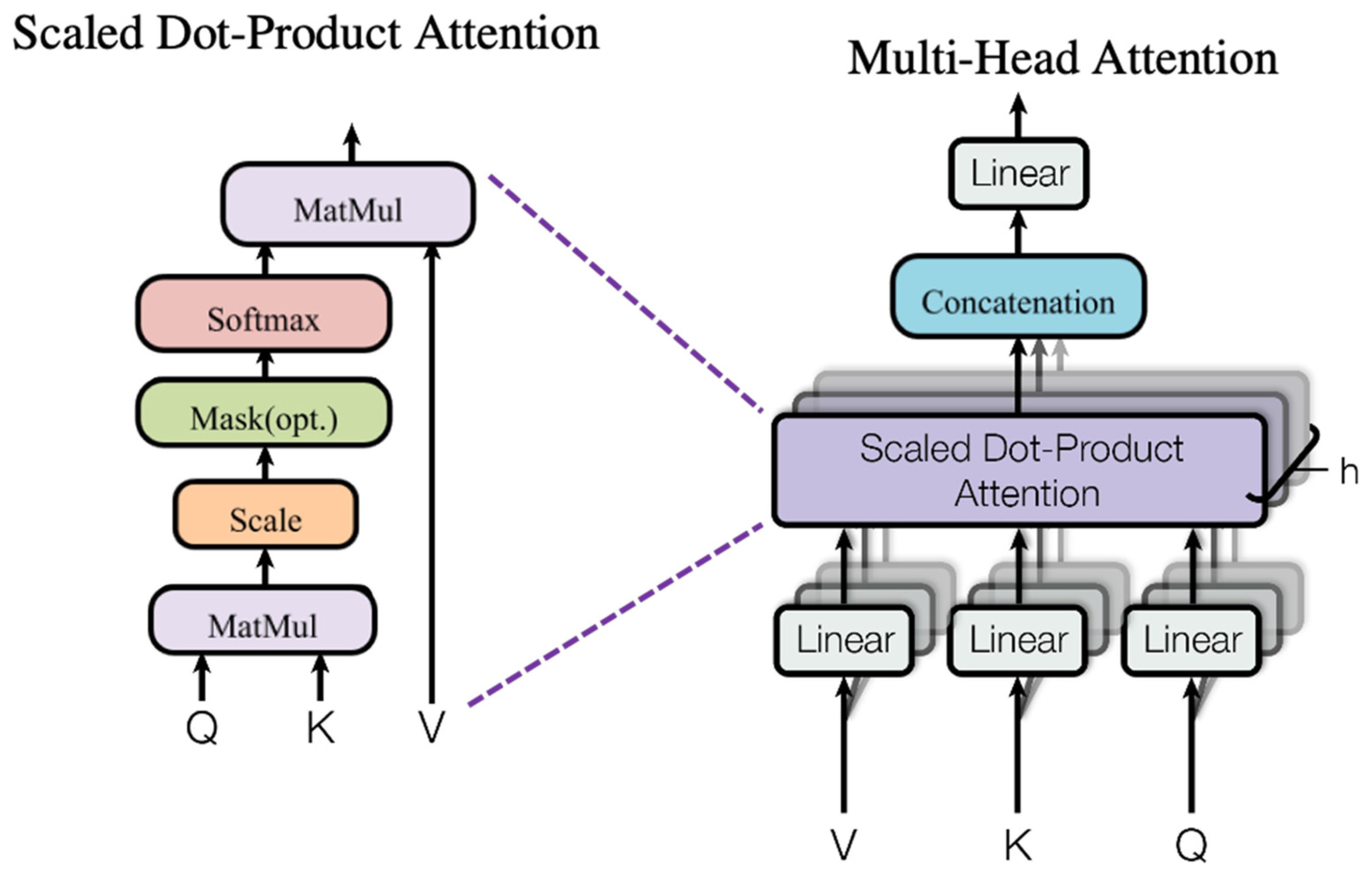
2.3. Multi-Head Self-Attention Module

To capture global dependencies, DFAST introduces the multi-head self-attention mechanism from the Transformer model [37], as shown in Figure 3. Assume that the input sequence is denoted as $F\in R^{L\times D}$, where L represents the sequence length, and D is the feature dimension.

First, the input features are linearly transformed to generate Query (Q), Key (K), and Value (V) matrices:

$$Q=F{W}_Q, K=F{W}_K, V=F{W}_V$$

(10)

where $W_Q,W_K,W_V$ are trainable weight matrices.

Next, the similarity between Query and Key is computed using a dot-product operation, resulting in the attention score matrix A:

$$A={\displaystyle \frac{Q{K}^{\top }}{\sqrt{d_k}}}$$

(11)

Here, $d_k$ is the dimension of the Key vector, included as a scaling factor to prevent excessively large dot-product values.

The attention scores $A$ are normalized using the Softmax function to generate the attention weight matrix $W$:

$$W=\mathit{softmax}\left(A\right)$$

(12)

Finally, the attention weight matrix $W$ is used to weight the value matrix $V$, producing the output features $O$:

$$O=WV$$

(13)

The multi-head attention mechanism divides the input data into multiple subspaces, computes attention independently for each subspace, and then concatenates and fuses the results. This approach enhances the model’s ability to capture diverse features.

This mechanism not only captures complex dependencies between spectral channels but also fully exploits the global properties of hyperspectral images, providing stronger representational power for classification tasks.

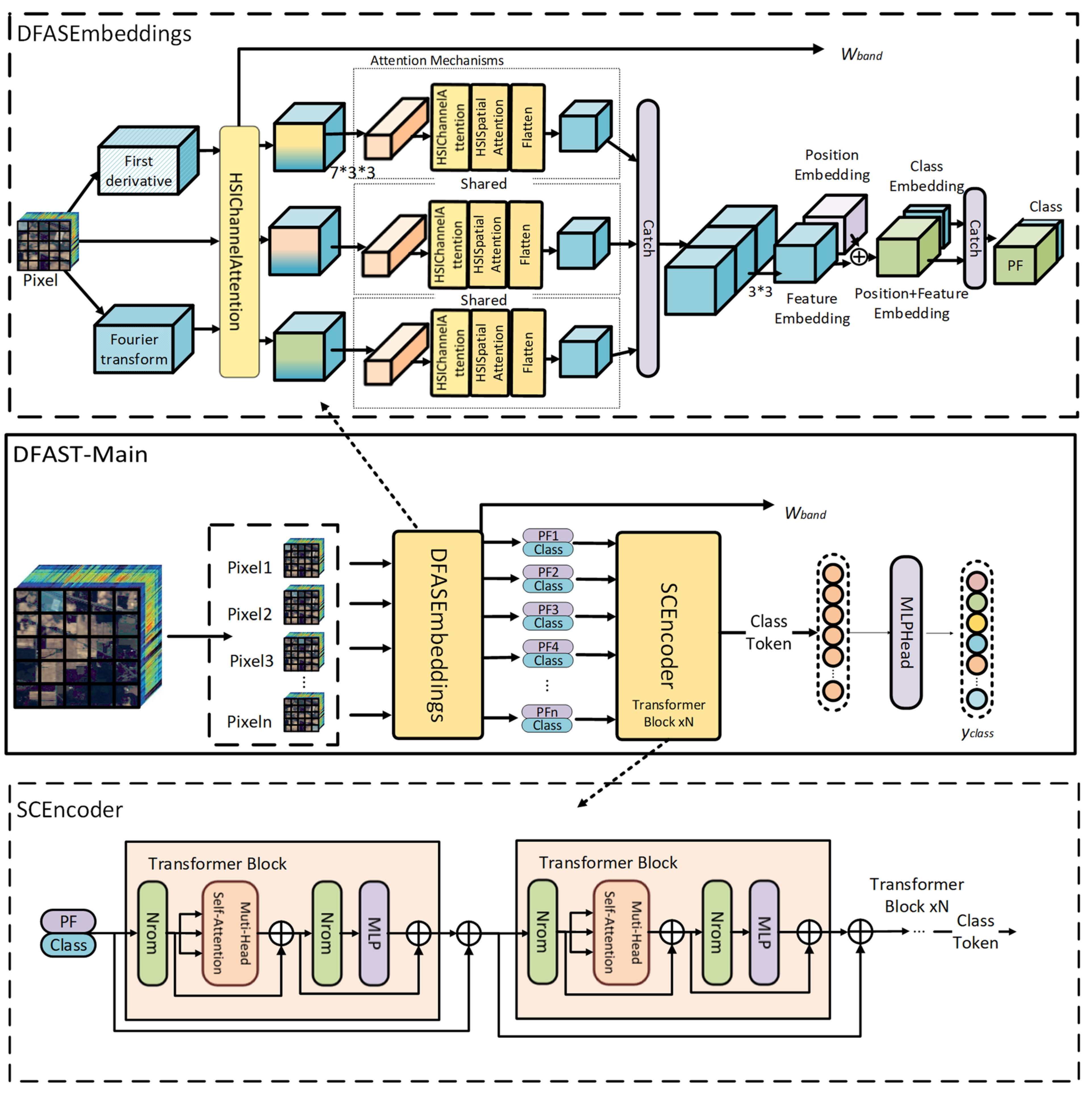
3. Method

This paper proposes DFAST for HSI classification, as illustrated in Figure 4. The proposed method includes DFASEmbeddings that extract raw spectral, first-order derivative, and frequency domain features through a multi-branch spectral attention structure. Each branch uses a shared-weight spectral attention module (HSIChannelAttention) for band selection, resulting in raw spectral, first-order derivative, and frequency domain attention features. The algorithmic pseudocode is presented in Algorithm 1.

Algorithm 1 Learning procedure for DFAST.
Input: Hyperspectral image tensor $x_i\in X$ with shape (H, W, C); training epochs T;
Output: Predicted labels $y_{\mathit{class}}$ band importance weights $w_{\mathit{band}}$
1:	While Epoch ≤ T do
2:	Initialize network parameters Θ
3:	Normalize input X channel-wise to obtain normalized data using ${\tilde{x}}_i={\displaystyle \frac{x_i}{\sqrt{\sum _{j=1}^C x_j^2+ϵ}}}$
4:	Raw Spectral Branch: $F_{\mathrm{raw}}={\tilde{x}}_i$
5:	First Derivative Branch: $F_{\mathit{grad}}={\tilde{x}}_i^{’}={\tilde{x}}_{i+1}-{\tilde{x}}_i$
6:	Frequency Domain Branch: $F_{\mathrm{freq}}=\left|FFT\left(\tilde{X}\right)\right|$
7:	Apply shared-weight HSIChannelAttention to $F_{\mathrm{raw}}$, $F_{\mathrm{grad}}$ and $F_{\mathrm{freq}}$ output $F_{01}$, $F_{02}$, $F_{03}$
8:	$\hspace{1em}{F}_{01}$, $F_{02}$ and $F_{03}$ are processed through shared-weight Attention Mechanisms to output $F_{11}$, $F_{12}$ and $F_{13}$
9:	Concatenate: $F_{\mathrm{f}\mathrm{u}\mathrm{s}\mathrm{e}\mathrm{d}}$= Concat($F_{11}$, $F_{12}$, $F_{13}$)
10:	Apply 3D convolution + Positional Encoding ${\to F}_{\mathit{embed}}=3\mathit{DConv}\left(F_{\mathrm{f}\mathrm{u}\mathrm{s}\mathrm{e}\mathrm{d}}\right)+\mathit{PosEncoding}$
11:	Append learnable class token cls to $F_{\mathit{embed}}$
12:	$\hspace{1em}{F}_{\mathit{embed}}$ is processed through the SCEncoder module to obtain $\mathit{ClassToken}$.
13:	Predict label: $y_{\mathit{class}}=\mathit{MLP}\left(\mathit{ClassToken}\right)$
14:	Update Θ by minimizing Loss($y_{\mathit{class}}$)
15:	end while

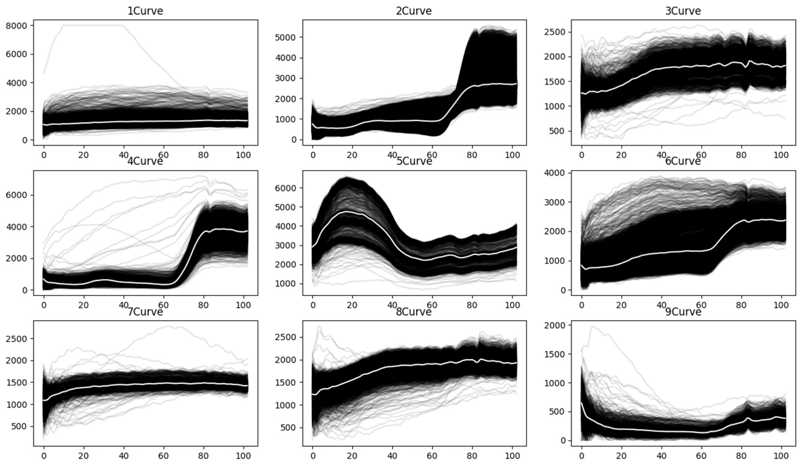
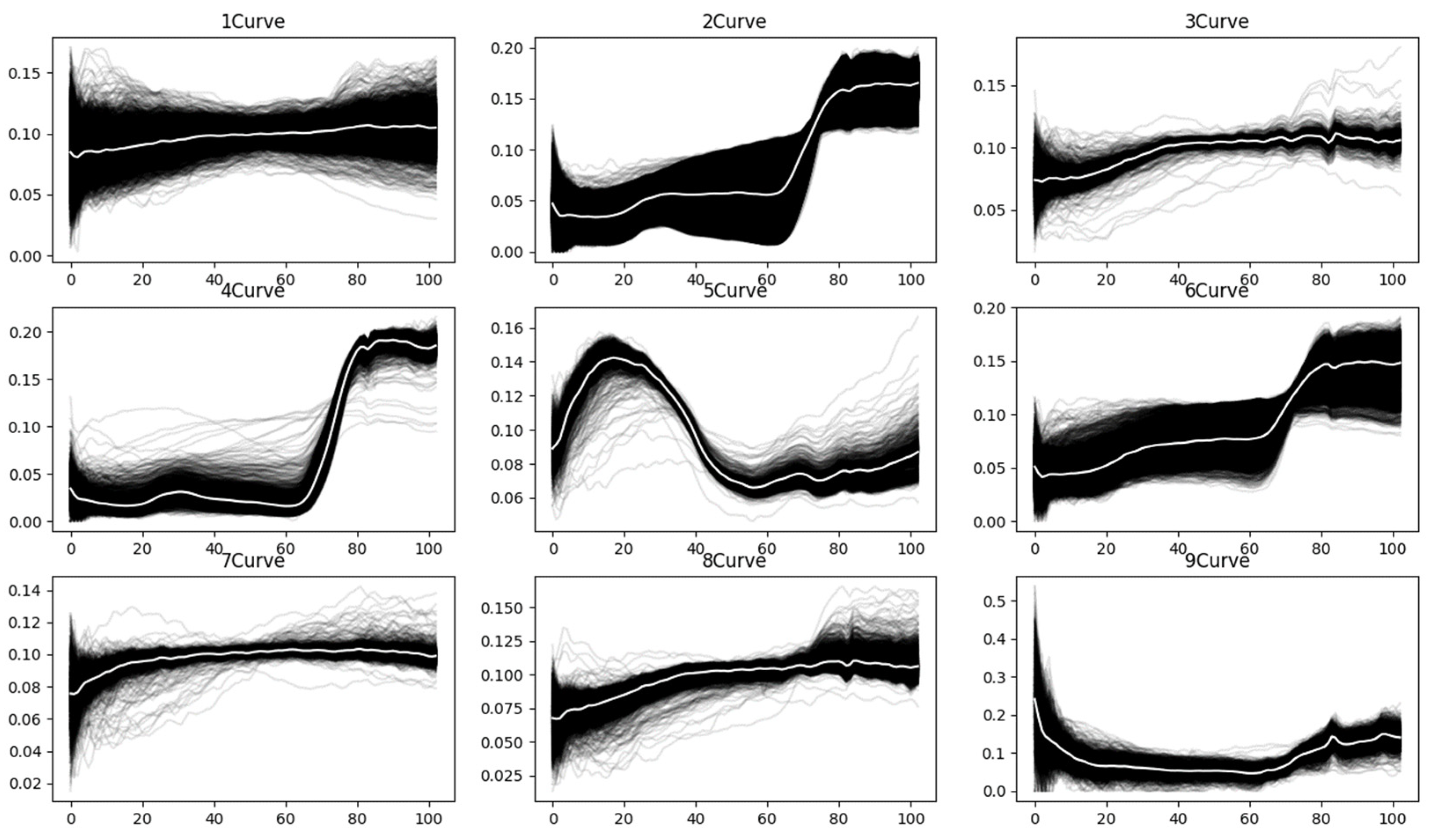
To better understand the characteristics of spectral curves, the raw spectral curves for each land-cover class in the PaviaU [39] hyperspectral dataset are plotted, as shown in Figure 5. The white line represents the mean spectral curve of all curves within each class. As illustrated in the figure, due to the influence of noise, various spectral curves significantly deviate from the majority of curves within the same class.

To prevent these noise-affected curves from being misclassified as other classes, we further apply channel normalization to the spectral curves, as shown in Figure 6.

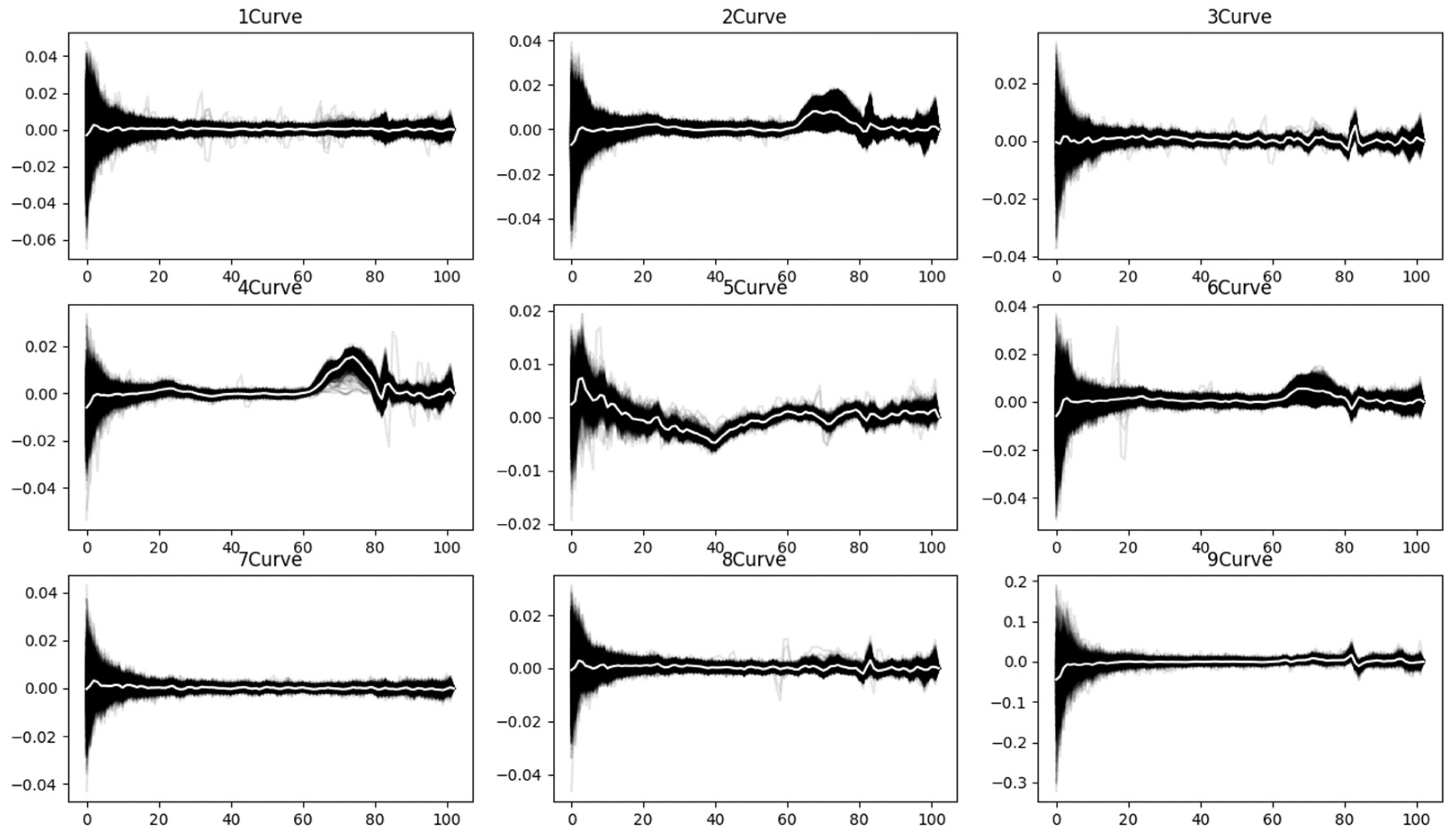
To further capture the variation trends in the spectral curves, the first derivative curves are extracted, as shown in Figure 7. This approach enhances the ability to analyze changes in the spectral curve more effectively.

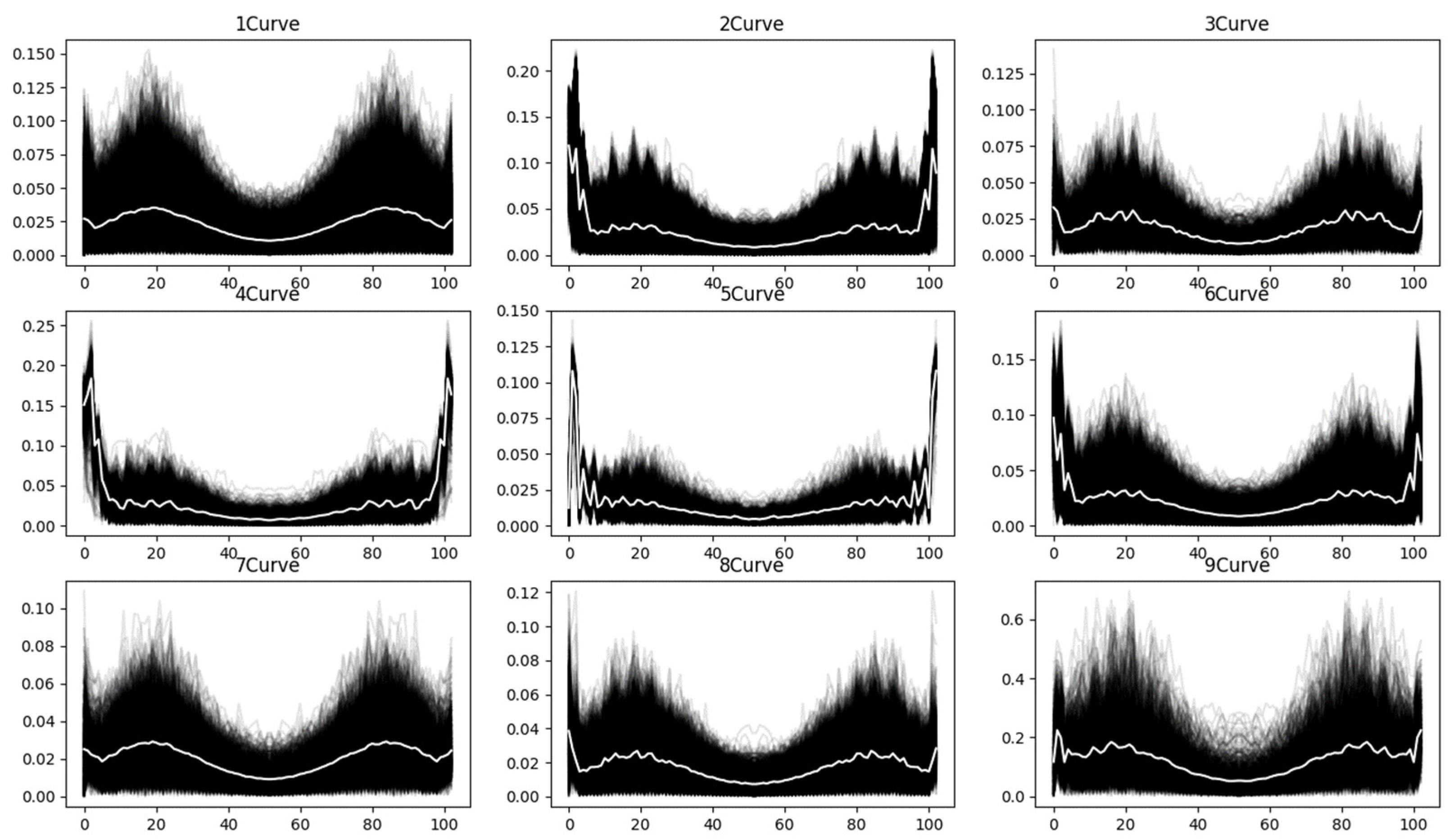
The frequency domain curves obtained after applying the Fourier transform to the spectral curves are shown in Figure 8. This transformation provides insights into the frequency characteristics of the spectral data, highlighting patterns and noise components in the frequency domain.

From the above curve diagrams, it can be observed that the gradient curves calculated after normalizing the spectral curves and the Fourier-transformed frequency domain curves extract spectral features from the perspectives of curve variation trends and the frequency domain, respectively. This process makes the distribution of all spectral curves within each class more concentrated, effectively reducing the impact of noise on classification results.

At the theoretical level, first-order derivative features enhance the saliency of diagnostic absorption characteristics of materials by capturing the reflectance variation rates between adjacent spectral bands, particularly in delineating key spectral signatures such as the vegetation red-edge transition zone and mineral absorption peaks. Taking vegetation classification as an example, the derivative processing accentuates distinctive patterns like the chlorophyll absorption trough at 550 nm and the steep slope variations in the red-edge region around 700 nm, while simultaneously suppressing multiplicative noise caused by illumination variations. The frequency domain features, obtained through Fourier transform, decompose spectral curves into different frequency components, where low-frequency elements represent the macroscopic reflectance properties of materials, and high-frequency components correspond to diagnostic subtle features (e.g., minor fluctuations of carbonate minerals at 2.3 μm).

The raw spectral, first-order derivative, and frequency domain attention features are then passed through a shared-weight feature encoding module. This module performs 3D convolution on the input attention features, followed by fine-grained spectral and spatial modeling using spectral attention and spatial attention (HSISpatialAttention) mechanisms. The encoded features from the three branches are subsequently fused and processed through a 2D convolution layer to generate embedded features, effectively reducing spectral redundancy and enhancing spatial dependencies. The embedded features, combined with positional embeddings, further capture the global dependencies of spectral and spatial features. By introducing a Learnable Class Token, the method aggregates features into feature-class embeddings.

The feature-class embeddings are input into an SCEncoder, where stacked Transformer layers capture global dependencies of spectral and spatial features, allowing the deep modeling of spectral–spatial coupling information. To address the challenges of increased network depth and gradient vanishing issues due to the cascaded modules, residual connections are introduced to ensure stable training. The output Class Token serves as the classification attention feature, which is passed through the classification head (MLPHead) to map the Class Token to category labels, thus completing the HSI classification task. The band selection weights, trained with the guidance of classification labels, are also generated as output to facilitate dimensionality reduction for hyperspectral images, effectively reducing network parameters, speeding up training, and improving classification accuracy.

3.1. Data Normalization

The input hyperspectral data $X\in R^{C\times H\times W}$ is a 3D tensor, where C represents the number of spectral bands, and H and W denote the height and width of the image, respectively. To eliminate numerical differences between spectral components, channel normalization is performed before processing. The normalization formula is as follows:

$${\tilde{x}}_i={\displaystyle \frac{x_i}{\sqrt{\sum _{j=1}^C x_j^2+ϵ}}}$$

(14)

Here, $x_i$ is the spectral value of the i-th channel for a given pixel, and ε is a small positive constant to avoid division by zero. The normalized value ${\tilde{x}}_i$ is used for subsequent feature extraction. This step standardizes the spectral data and reduces variability among features.

3.2. Feature Extraction

To obtain multi-dimensional feature information, the proposed method employs a multi-branch structure:

1.

Raw Spectral Branch: This branch directly uses the normalized spectral data $\tilde{X}$ as input. This approach preserves the raw spectral information, providing a foundational input for the model.

$$F_{\mathrm{raw}}={\tilde{x}}_i$$

(15)

2.

First Derivative Branch: This branch aims to capture local variation trends in the spectral curve. Specifically, it computes the first-order derivative of the normalized spectral data $\tilde{X}$ for each channel:

$$F_{\mathrm{grad}}={\tilde{x}}_i^{’}={\tilde{x}}_{i+1}-{\tilde{x}}_i$$

(16)

Here, ${\tilde{x}}_i^{’}$ represents the rate of change between the i-th and (i+1)-th spectral channels. By calculating the derivative information of the spectral curve, this branch extracts the variation characteristics of spectral data, which is particularly useful for recognizing targets with significant variation trends.

3.

Frequency Domain Branch: This branch extracts frequency domain features by applying the Fourier transform to the normalized spectral data $\tilde{X}$. The spectral data is transformed, and the magnitude of the Fourier coefficients is used as the feature input:

$$F_{\mathrm{freq}}=\left|\mathcal{F}\left(\tilde{X}\right)\right|$$

(17)

Here, $\mathcal{F}$ represents the Fourier transform, and |·| denotes the magnitude operation. This process captures global spectral characteristics in the frequency domain, such as periodicity and frequency distribution.

In the frequency domain feature design, we opt to retain only the magnitude spectrum of the Fourier transform while discarding phase information. This decision is grounded in two key scientific considerations: First, hyperspectral material discrimination primarily relies on energy distribution characteristics. Empirical measurements demonstrate that diagnostic features such as the chlorophyll absorption trough (650 nm) and water absorption band (1450 nm) exhibit prominent and stable representation in the magnitude spectrum, whereas statistical tests confirm the insignificant contribution of phase information to classification accuracy. Second, phase information proves more susceptible to sensor noise. Simulation experiments reveal that under Gaussian noise with SNR < 30 dB, the classification accuracy retention rate based on phase spectrum is markedly lower than that achieved using the magnitude spectrum.

The features extracted from these three branches are denoted as $F_{\mathrm{raw}}$, $F_{\mathrm{grad}}$, and $F_{\mathrm{freq}}$, respectively. Each branch’s data is passed through a shared-weight learnable HSIChannelAttention module to obtain band-selected outputs $w_{\mathit{band}}$ for the three branches. This multi-branch feature extraction method retains the raw spectral information, local variation characteristics, and frequency domain features, providing a comprehensive feature representation for subsequent modeling.

3.3. Attention Mechanisms

To enhance feature expressiveness, HSI Channel Attention is introduced. For the input features $F$ of each branch, maximum pooling and average pooling are performed along the channel dimension to generate spectral descriptors:

$$F_{\mathit{max}}=\mathit{MaxPool}\left(F\right), F_{\mathit{avg}}=\mathit{AvgPool}\left(F\right)$$

(18)

Here, $\mathrm{MaxPool}$ and $\mathrm{AvgPool}$ represent maximum pooling and average pooling operations, respectively. The results $F_{\max }$ and $F_{\mathrm{avg}}$ are used to generate channel attention weights. The attention weights are computed using fully connected layers as follows:

$$W_c=\sigma \left({\mathit{FC}}_2\left(\mathit{ReLU}\left({\mathit{FC}}_1\left(F_{\mathit{max}}+F_{\mathit{avg}}\right)\right)\right)\right)$$

(19)

Here, ${\mathit{FC}}_1$ and ${\mathit{FC}}_2$ are two fully connected layers, and $\sigma$ is the Sigmoid activation function. The weights $W_c$ represent the importance of each channel and are applied to the input features:

$$F_c=F\odot W_c$$

(20)

where ⊙ denotes element-wise multiplication. The channel attention mechanism adaptively adjusts the weights of different channels, emphasizing important spectral features.

To capture spatial characteristics of the image, HSI Spatial Attention is applied to the channel-weighted features $F_c$. Global average pooling and maximum pooling are performed along the channel dimension, and the results are concatenated:

$$F_s=\sigma \left(\mathit{Conv}([\mathit{MaxPool}(F_c),\mathit{AvgPool}(F_c)])\right)$$

(21)

Here, $\mathrm{Conv}$ represents a convolution operation, and $[\cdot ,\cdot ]$ denotes concatenation along the channel dimension. The result $F_s$ is a spatial weight matrix used to weight the features:

$$F_{\mathit{spatial}}=F_c\odot F_s$$

(22)

This mechanism highlights key spatial regions in the image, further improving the precision of feature representation.

3.4. Feature Fusion and Embedding

The outputs of the three branches $F_{\mathit{spatiaRaw}}$, $F_{\mathit{spatiaGrad}}$, and $F_{\mathit{spatiaFreq}}$ are concatenated to form a multi-branch input:

$$F_{\mathit{ALLspatial}}=\left[F_{\mathit{spatiaRaw}},F_{\mathit{spatiaGrad}},F_{\mathit{spatiaFreq}}\right]$$

(23)

The concatenated features are passed through a 3D convolution layer to extract fine-grained spectral–spatial features. Positional encoding is added to the feature map to form the final embedded features:

$$F_{\mathit{embed}}=3\mathit{DConv}\left(F_{\mathit{ALLspatial}}\right)+\mathit{PosEncoding}$$

(24)

PosEncoding refers to learnable positional encoding, which assigns a set of trainable parameters to each spatial position in the input feature map. This mechanism enables the model to autonomously learn positional information from the data during training. Unlike fixed mathematical functions (e.g., sine/cosine encodings), PosEncoding optimizes position representations via backpropagation, allowing it to adapt to the specific requirements of the task.

Last, we append learnable class token cls to $F_{\mathit{embed}}$ to obtain new $F_{\mathit{embed}}$ for the Classification task.

3.5. Transformer Encoder for Global Feature Modeling

In the Transformer encoder, the embedded features $F_{\mathrm{embed}}$ are used as input to capture global dependencies between spectral and spatial features through the multi-head attention mechanism. First, the embedded features are linearly transformed into Query (Q), Key (K), and Value (V) vectors:

$$Q=W_Q{F}_{\mathit{embed}}, K=W_K{F}_{\mathit{embed}}, V=W_V{F}_{\mathit{embed}}$$

(25)

where $W_Q$, $W_K$, and $W_V$ are trainable weight matrices used to generate the Query, Key, and Value vectors. The attention weights are computed using the scaled dot-product attention formula:

$$\mathrm{Attention}\left(Q,K,V\right)=\mathrm{softmax}\left({\displaystyle \frac{Q{K}^{\top }}{\sqrt{d_k}}}\right)V$$

(26)

Here, $d_k$ represents the dimension of the Key vector and is used as a normalization factor to prevent excessively large dot-product values, which could lead to gradient vanishing issues. The $\mathrm{softmax}$ operation normalizes the attention scores, which are then used to weight the Value vector $V$, extracting the global correlation features.

The multi-head attention mechanism computes attention in parallel across h attention heads, allowing the model to focus on different subspaces of the input features. The output of the multi-head attention is computed as follows:

$${\mathit{head}}_i=\mathrm{Attention}\left(Q{W}_Q^i,K{W}_K^i,V{W}_V^i\right)$$

(27)

$$\mathrm{MultiHead}\left(Q,K,V\right)=\mathrm{Concat}\left({\mathit{head}}_1,\dots ,{\mathit{head}}_h\right)W_O$$

(28)

$W_Q^i$, $W_K^i$, and $W_V^i$ are the projection matrices specific to the i-th head, and $W_O$ is a weight matrix used for the final linear transformation of the concatenated attention outputs.

The output of the multi-head attention mechanism is combined with the original input $F_{\mathit{embed}}$ using a residual connection to ensure gradient flow and training stability. Layer normalization is then applied to normalize the feature distribution:

$$F_{\mathit{updated}}=\mathit{LayerNorm}\left(F_{\mathit{embed}}+\mathit{MultiHead}\left(Q,K,V\right)\right)$$

(29)

After passing through N layers of the Transformer encoder, the global spectral and spatial features are extracted and used for classification and dimensionality reduction.

3.6. Classification and Dimensionality Reduction

At the classification and dimensionality reduction stage, the updated features $F_{\mathrm{updated}}$ = $\{\mathit{ClassToken},\dots \}$ are further processed. The $\mathrm{ClassToken}$, which aggregates information from all features, is used to generate the classification output $y_{\mathrm{class}}$:

$$y_{\mathit{class}}=\mathit{MLP}\left(\mathit{ClassToken}\right)$$

(30)

Here, the $\mathit{MLP}$ is a multi-layer perceptron that maps the $\mathit{ClassToken}$ to specific category labels.

Additionally, the HSIChannelAttention weights $w_{\mathit{band}}$ are used to evaluate the importance of each spectral band. The importance of spectral bands is computed as the average attention weights across all Transformer layers.

The workflow of the entire system, from hyperspectral data input to the final classification and band weight output, consists of several key steps: data normalization, multi-branch feature extraction, channel and spatial attention modeling, embedded feature extraction, and global feature optimization using the Transformer encoder. Finally, the classification head generates the classification result $y_{\mathrm{class}}$, while the attention weights are used to extract the importance of spectral bands as $w_{\mathrm{band}}$. This system design fully leverages the spectral and spatial characteristics of hyperspectral data and uses deep learning models for efficient multi-dimensional feature modeling, achieving both hyperspectral image classification and dimensionality reduction tasks.

This system is designed to fully utilize the spectral and spatial properties of hyperspectral data while leveraging deep learning models for effective multi-dimensional feature modeling. By combining spectral and spatial attention mechanisms, multi-branch feature extraction, and Transformer-based global feature modeling, the proposed method achieves efficient hyperspectral image classification and dimensionality reduction.

4. Experiments

4.1. Dataset

This study employed three publicly available standard hyperspectral datasets—Salinas, Pavia University, and Indian Pines. These benchmark datasets, accessible via [39], have been widely used in hyperspectral classification research, ensuring fair comparisons with existing methods. The selection of multi-regional datasets (covering California, USA; Pavia, Italy; and Indiana, USA) was designed to systematically validate the method’s generalization capability across different land cover types (such as crops, buildings, and natural vegetation). This is crucial for addressing geographic variability in spectral characteristics in practical applications.

1.

Salinas Dataset:

The Salinas dataset [39] was collected by the Airborne Visible Infrared Imaging Spectrometer (AVIRIS) sensor over Salinas Valley, California, and is characterized by a high spatial resolution of 3.7 m per pixel. The dataset consists of 224 spectral bands covering a wavelength range from 400 to 2500 nm. It contains 512 × 217 pixels, totaling 111,104 samples, with 16 different classes and 54,129 labeled samples. The dataset includes various landscapes such as vegetable fields, bare soil, and vineyards. The visualization of the Salinas dataset is shown in Figure 9a, and the corresponding ground truth is shown in Figure 9b.

2.

Pavia University Dataset:

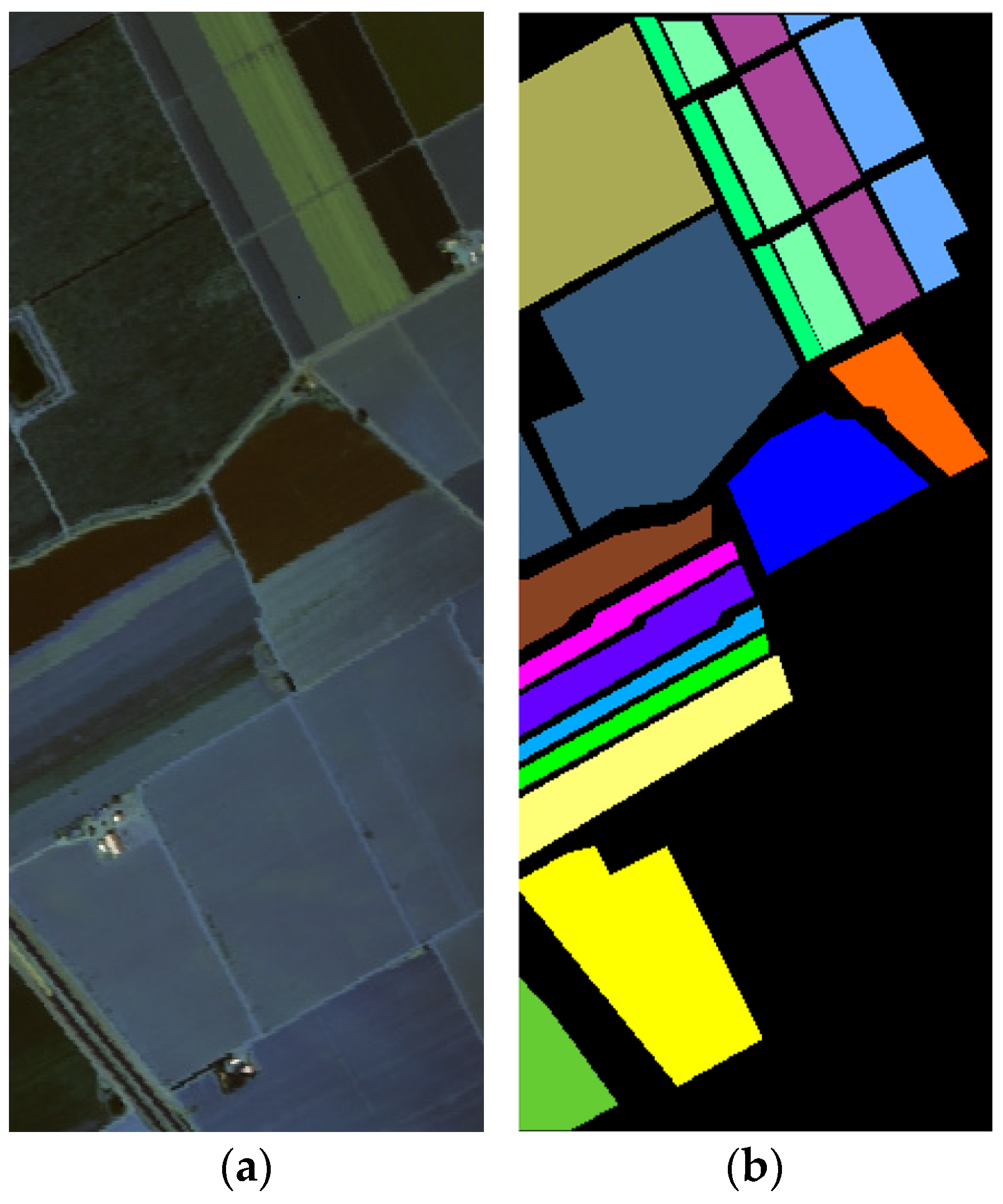
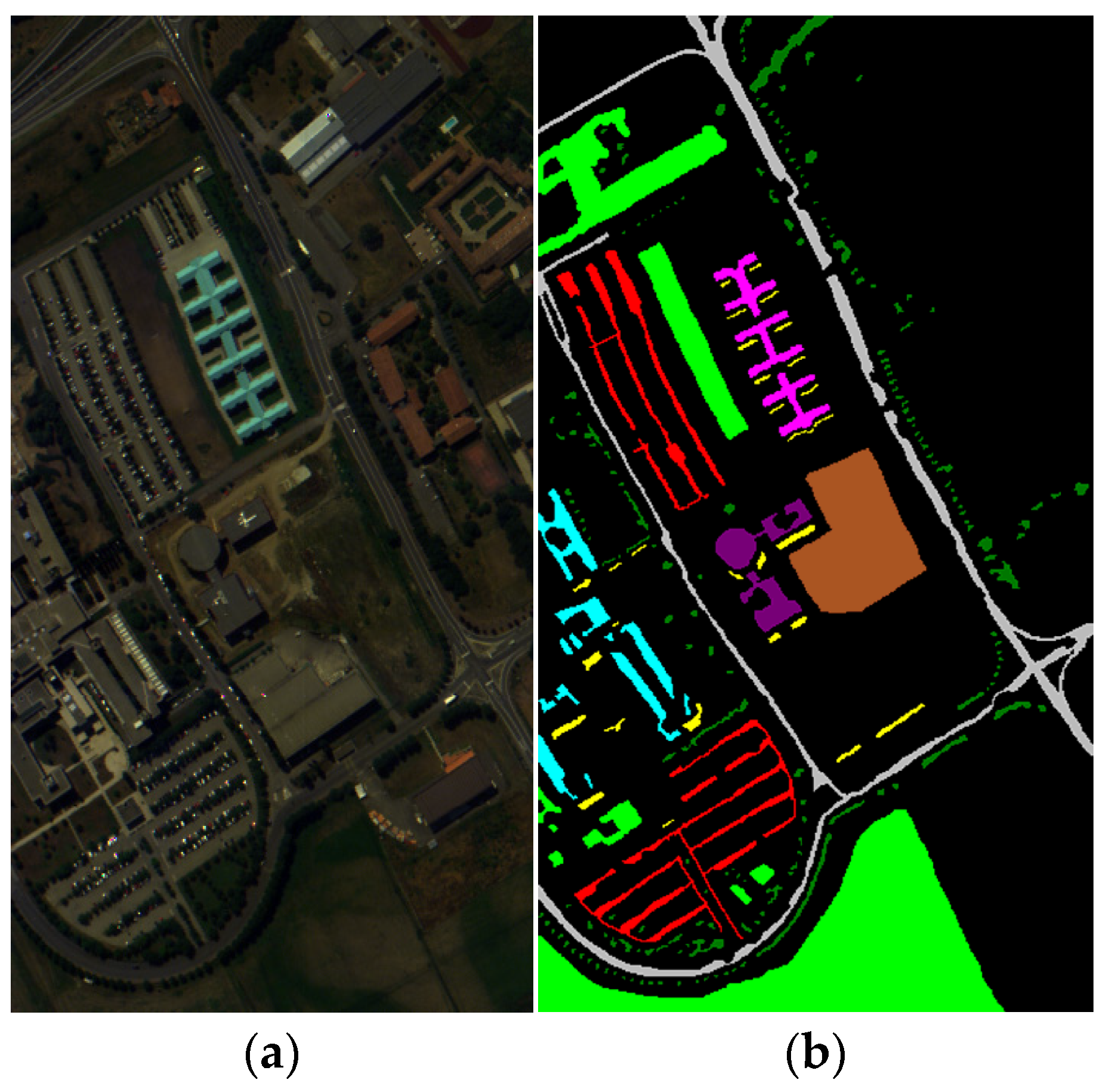
The Pavia University (PaviaU) [39] dataset was collected by the ROSIS-03 sensor over the urban area of Pavia, northern Italy. It has a high geometric resolution of 1.3 m per pixel and consists of 610 × 340 pixels, totaling 207,400 samples. Initially, the dataset included 115 spectral bands, but 12 bands were discarded due to noise, leaving 103 spectral bands for the experiments.

This dataset represents an urban landscape with 9 classes and 42,776 labeled samples, including various urban surfaces such as asphalt, bricks, grass, and trees. The visualization of the PaviaU dataset is shown in Figure 10a, and the corresponding ground truth is shown in Figure 10b.

3.

Indian Pines Dataset:

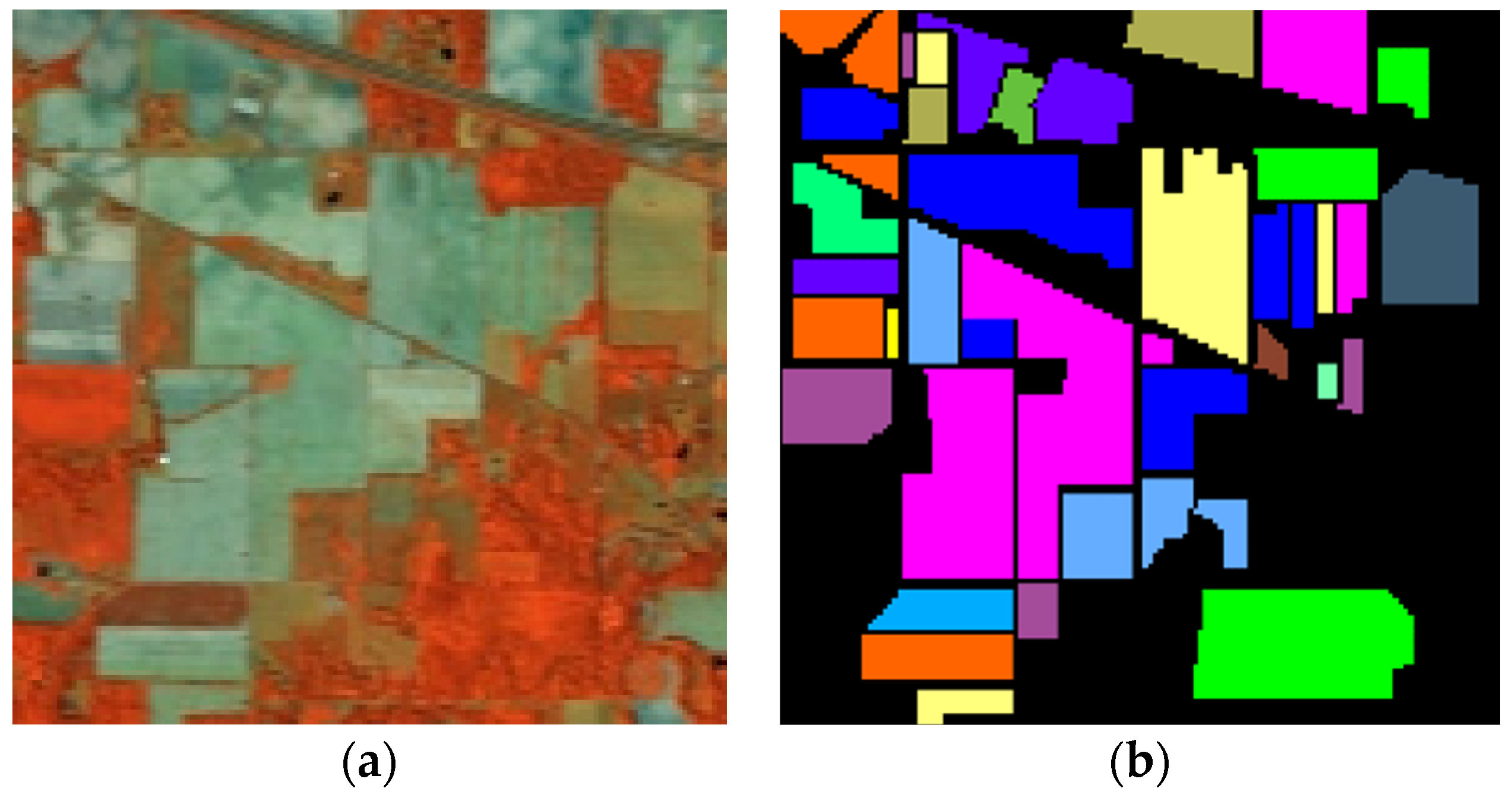
The Indian Pines dataset [39] was captured by the Airborne Visible/Infrared Imaging Spectrometer (AVIRIS) in 1992. It represents a 145 × 145 pixel region of the Indian Pines area in northwestern Indiana. The dataset consists of 21,025 samples and originally contained 224 spectral bands, spanning a wavelength range of 0.4 to 2.5 μm. For experiments, all 224 bands are retained. The spatial resolution of the dataset is 20 m per pixel.

This dataset is notable for its diverse class representation, which includes 16 different classes and a total of 10,249 labeled samples. The majority of the classes represent agricultural land and natural perennial vegetation.

The visualization of the Indian Pines dataset is shown in Figure 11a, and the corresponding ground truth is shown in Figure 11b.

4.2. Definition of Metrics

To comprehensively evaluate the performance of the classification model on hyperspectral images, three commonly used evaluation metrics are adopted in this paper: overall accuracy (OA), average accuracy (AA), and the Kappa coefficient [40].

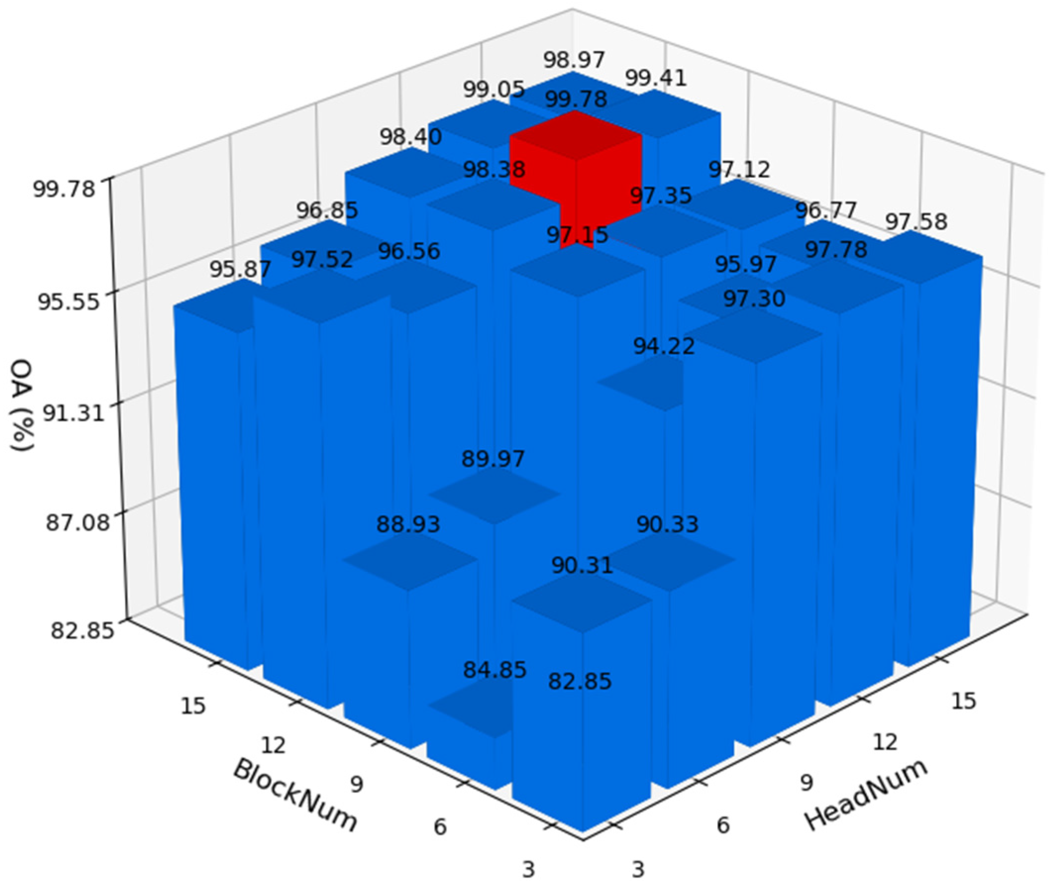
4.3. Parameter Analysis

Due to the use of multi-head attention and multiple Transformer blocks in the network architecture, experiments were designed to determine the optimal number of attention heads and Transformer blocks to optimize network performance. The test results on the Pavia University dataset are shown in Figure 12. It can be observed that when the number of heads (HeadNum) is set to 12 and the number of Transformer blocks (BlockNum) is also set to 12, the network achieves optimal accuracy on the Pavia University dataset.

When hyperspectral data is input into the network, it is partitioned to better capture spatial features. The network was tested with various patch sizes (patchSize), and the results are shown in

Table 1. Accuracy testing under different patch sizes.

Dataset	Metrics	PatchSize
		11	17	25	31
Salinas	OA (%)	98.40	99.67	99.96	99.79
	AA (%)	98.69	98.65	99.94	99.64
	Kappa (%)	98.33	99.58	99.95	99.68
Pavia University	OA (%)	97.56	99.35	99.78	99.49
	AA (%)	95.85	98.71	99.42	98.92
	Kappa (%)	96.76	99.09	99.71	99.32
Indian Pines	OA (%)	90.33	97.35	98.28	97.68
	AA (%)	83.86	94.26	96.51	94.77
	Kappa (%)	88.97	97.03	98.04	97.35

. It can be observed that when the patch size is 25, the network achieves the highest accuracy across all three datasets.

To determine the optimal learning rate for the network, various initial learning rates (lrs) were tested. The results are shown in

Table 2. Accuracy testing under different learning rates.

Dataset	Metrics	Learning Rate
		0.05	0.01	0.005	0.001
Salinas	OA (%)	98.39	99.53	99.79	99.96
	AA (%)	97.60	99.70	99.86	99.94
	Kappa (%)	98.22	99.49	99.81	99.95
Pavia University	OA (%)	96.16	98.75	99.49	99.78
	AA (%)	95.65	98.70	98.94	99.42
	Kappa (%)	94.57	98.18	98.41	99.71
Indian Pines	OA (%)	89.31	96.28	96.74	98.28
	AA (%)	85.76	95.14	95.95	96.51
	Kappa (%)	87.85	96.22	96.41	98.04

. It can be observed that when the initial learning rate is set to 0.001, the highest accuracy is achieved across all three datasets.

Based on the parameter testing experiments above, we ultimately selected HeadNum = 12, BlockNum = 12, patchSize = 25, and learning rate lr = 0.001 as the optimal parameters for the network.

4.4. Experimental Parameters

We constructed a hyperspectral image classification experimental framework based on the PyTorch 2.0.0 library. The experimental system was equipped with an NVIDIA GeForce RTX 4090 GPU with 24 GB of memory which was purchased from NVIDIA Corporation’s authorized distributor in Beijing, China and run in a Python 3.8 environment. The experimental parameters were configured as follows:

(a) General parameters: A training sample ratio of 0.1 per class, a batch size of 512, 300 training epochs, and the Adam optimizer [41] (learning rate = 0.001).

(b) Optimized parameters: As determined by the parameter analysis in Table 1 and Table 2, the patch size (PatchSize) was set to 25, the number of attention heads (HeadNum) in the multi-head attention mechanism was set to 12, and the number of blocks (BlockNum) was configured to 12 layers.

4.5. Comparative Analysis

To validate the effectiveness of DFAST, recognition experiments were conducted on the Salinas, Pavia University, and Indian Pines datasets. These were compared with traditional methods including SVM, convolutional networks (2DCNN, 3DCNN, HybridSN [42]), as well as Transformer-based networks (ViT, SpectralFormer, SSFTT, morphFormer). The numbers in parentheses indicate the error of five repeated experiments.

To validate the accuracy differences between the proposed method and graph neural networks, the latest graph neural network algorithms—Semi-Supervised Multiscale Dynamic Graph Convolution Network (DMSGer) [43], Context-Aware Dynamic Graph Convolutional Network (CAD-GCN) [44], and Multiscale Dynamic Graph Convolutional Network (MDGCN) [45]—were selected for comparison with the proposed method.

From

Table 3. Classification results on Salinas dataset comparing SVM, 2DCNN, 3DCNN, HybridSN, ViT, SpectralFormer, SSFTT, morphFormer, and the Proposed DFAST Network.

No	Class	Conventional Classifiers	Convolutional Networks			Transformer Networks
		SVM	2DCNN	3DCNN	HybridSN	ViT	Spectral Former	SSFTT	Morph Former	DFAST (Ours)
1	Weeds_1	97.61	99.80	99.45	100	99.75	100	99.95	100.0	100
2	Weeds_2	98.75	99.68	99.15	99.92	98.95	99.23	99.57	100.0	100
3	Fallow	93.04	99.79	97.37	99.34	95.90	98.20	99.35	99.85	100
4	Fallow_plow	94.73	98.02	98.30	99.57	99.07	97.55	99.35	99.15	99.36
5	Fallow_smooth	81.38	98.81	94.59	99.18	98.44	99.32	99.40	99.85	99.85
6	Stubble	99.97	99.40	99.27	100	99.97	99.90	99.67	99.97	99.95
7	Celery	99.92	100	100	99.97	98.44	99.39	99.97	99.97	100
8	Grapes	88.17	90.57	89.54	94.36	88.25	90.16	94.17	99.80	99.94
9	Soil	99.45	99.68	98.41	99.89	98.97	99.71	99.58	99.87	100
10	Corn	90.62	97.76	86.80	99.66	91.65	98.91	98.44	99.72	100
11	Lettuce 4wk	95.08	97.95	93.12	98.8	97.48	95.30	97.97	98.05	100
12	Lettuce 5wk	98.5	93.45	69.33	99.74	98.74	99.63	99.74	100	100
13	Lettuce 6wk	98.98	92.05	85.96	96.21	97.84	99.23	99.36	99.89	100
14	Lettuce 7wk	55.04	98.79	87.44	98.55	98.31	98.88	86.96	100	100
15	Vineyard_U	81.04	90.42	85.92	93.43	81.25	89.52	95.50	99.33	99.97
16	Vineyard_T	94.61	99.60	97.29	99.83	98.03	99.50	99.50	100	100
OA (%)		90.91 (0.01)	95.93 (0.23)	92.37 (0.21)	97.69 (0.65)	93.75 (0.22)	95.60 (0.31)	97.54 (0.12)	99.73 (0.07)	99.96 (0.02)
AA (%)		88.22 (0.01)	96.79 (0.12)	90.52 (0.10)	98.68 (0.52)	96.42 (0.13)	96.05 (0.25)	97.89 (0.26)	99.75 (0.12)	99.94 (0.03)
Kappa (%)		89.88 (0.01)	95.47 (0.15)	91.51 (0.13)	97.43 (0.75)	93.05 (0.25)	97.83 (0.22)	97.26 (0.31)	99.78 (0.10)	99.95(0.02)

The bolded ones indicate the optimal.

,

Table 4. Classification results on Pavia University dataset comparing SVM, 2DCNN, 3DCNN, HybridSN, ViT, SpectralFormer, SSFTT, morphFormer, and the Proposed DFAST Network.

No	Class	Conventional Classifiers	Convolutional Networks			Transformer Networks
		SVM	2DCNN	3DCNN	HybridSN	ViT	Spectral Former	SSFTT	Morph Former	DFAST (Ours)
1	Asphalt	92.32	94.00	97.50	98.58	95.35	93.55	99.28	99.14	99.62
2	Meadows	98.88	99.95	98.95	99.37	98.54	92.78	99.76	99.98	99.99
3	Gravel	87.73	85.18	88.07	96.86	95.28	89.64	93.85	98.73	100
4	Trees	98.17	98.83	98.08	99.57	99.60	95.91	99.54	99.25	98.52
5	Metal Sheets	96.62	100	99.26	99.85	99.85	100	100	100	99.70
6	Bare Soil	95.10	96.00	99.51	99.76	91.88	92.13	99.76	97.63	99.96
7	Bitumen	53.17	82.14	73.44	96.27	82.15	84.14	94.49	99.31	99.85
8	Bricks	75.80	91.47	86.78	87.95	90.40	83.54	90.67	92.05	99.65
9	Shadows	00.00	99.71	97.28	99.78	99.06	98.41	99.78	99.89	99.78
OA (%)		92.41 (0.02)	96.40 (0.25)	95.64 (0.51)	98.03 (0.08)	95.94 (0.16)	92.12 (0.17)	98.41 (0.49)	98.70 (0.08)	99.78 (0.02)
AA (%)		80.31 (0.01)	91.99 (0.16)	91.23 (0.67)	95.94 (0.07)	95.07 (0.15)	89.70 (0.07)	97.08 (0.87)	97.93 (0.02)	99.42 (0.02)
Kappa (%)		89.93 (0.02)	95.24 (0.17)	93.46 (0.52)	97.39 (0.06)	94.63 (0.13)	99.45 (0.18)	97.89 (0.90)	98.28 (0.09)	99.71 (0.02)

The bolded ones indicate the optimal.

,

Table 5. Classification results on Indian Pines dataset comparing SVM, 2DCNN, 3DCNN, HybridSN, ViT, SpectralFormer, SSFTT, morphFormer, and the Proposed DFAST Network.

No	Class	Conventional Classifiers	Convolutional Networks			Transformer Networks
		SVM	2DCNN	3DCNN	HybridSN	ViT	Spectral Former	SSFTT	Morph Former	DFAST (Ours)
1	Alfalfa	00.00	91.11	97.50	100	00.00	00.00	97.22	97.78	100
2	CornN	73.16	94.64	89.29	96.89	75.47	64.83	93.65	98.32	99.06
3	CornM	63.05	87.32	81.83	88.03	62.07	55.33	92.46	95.57	96.93
4	Corn	96.67	91.04	80.43	92.23	85.00	45.73	92.08	78.31	99.15
5	GrassM	97.14	96.30	97.67	96.54	80.78	75.58	98.54	99.17	99.59
6	GrassT	90.69	98.61	97.95	98.49	94.72	81.73	99.04	99.59	97.72
7	GrassP	00.00	00.00	00.00	0.00	00.00	00.00	100	100	90.32
8	HayW	92.10	98.76	95.98	98.96	84.84	85.59	98.35	98.35	100
9	Oats	00.00	100	00.00	100	00.00	00.00	76.47	100	83.33
10	SoybeanN	73.97	90.03	92.34	90.69	79.22	26.83	96.06	95.33	98.66
11	SoybeanM	80.30	94.86	89.18	92.92	72.89	60.87	96.39	99.54	97.56
12	SoybeanC	61.62	91.58	91.22	94.31	77.58	49.28	90.95	93.55	96.73
13	Wheat	48.92	90.45	91.86	87.34	94.86	77.19	98.51	97.13	100
14	Woods	89.88	97.71	97.99	97.72	82.77	93.84	98.51	98.73	98.98
15	Buildings	66.02	90.37	85.54	91.04	89.97	68.06	96.82	97.22	99.46
16	Stone	00.00	90.20	80.18	90.20	86.14	100	85.19	97.73	97.70
OA (%)		77.78 (0.30)	93.96 (0.36)	90.96 (0.59)	94.07 (0.06)	77.98 (0.69)	68.37 (0.74)	95.80 (0.11)	97.34 (0.71)	98.28 (0.02)
AA (%)		55.05 (0.19)	83.21 (0.07)	79.52 (0.31)	83.58 (0.42)	62.91 (0.56)	50.34 (0.41)	92.23 (0.5)	92.87 (0.02)	96.51 (0.01)
Kappa (%)		74.52 (0.41)	93.12 (0.10)	89.67 (0.16)	93.23 (0.66)	74.66 (0.73)	63.38 (0.81)	95.22 (0.97)	96.97 (0.88)	98.04 (0.02)

The bolded ones indicate the optimal.

and

Table 6. Classification accuracy (%) comparison with dynamic graph convolutional networks.

OA (%)	Graph-Based Methods
	MDGCN	CAD-GCN	DMSGer	DFAST (Ours)
Salinas	97.25 (0.87)	98.28 (0.54)	99.65 (0.06)	99.96 (0.02)
Pavia University	95.68 (0.22)	92.91 (1.01)	96.73 (0.48)	99.78 (0.02)
Indian Pines	93.47 (0.38)	94.13 (0.78)	95.39 (0.21)	98.28 (0.02)

, it can be observed that the proposed DFAST hyperspectral classification method achieved OA% values of 99.96, 99.78, and 98.28 on the Salinas, Pavia University, and Indian Pines datasets, respectively. In comparison, the best-performing competing method, morphFormer, achieved OA% values of 99.73, 98.70, and 97.34 on the same datasets, reflecting improvements of 0.23, 1.08, and 0.94, respectively. 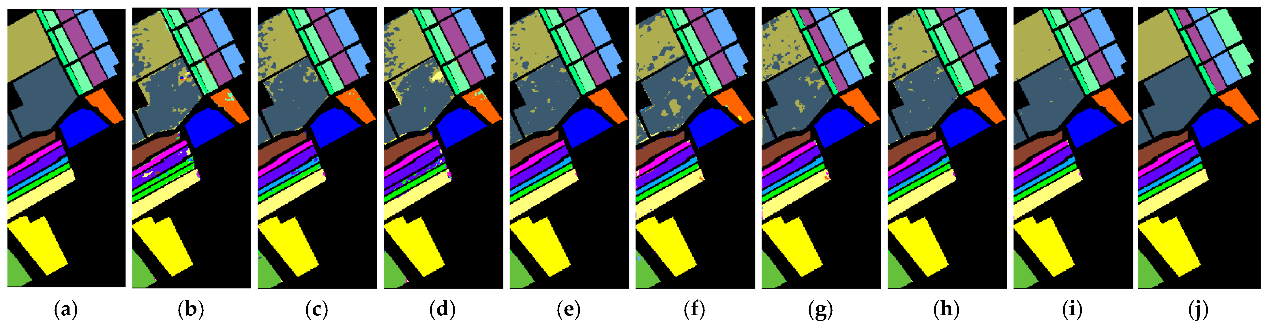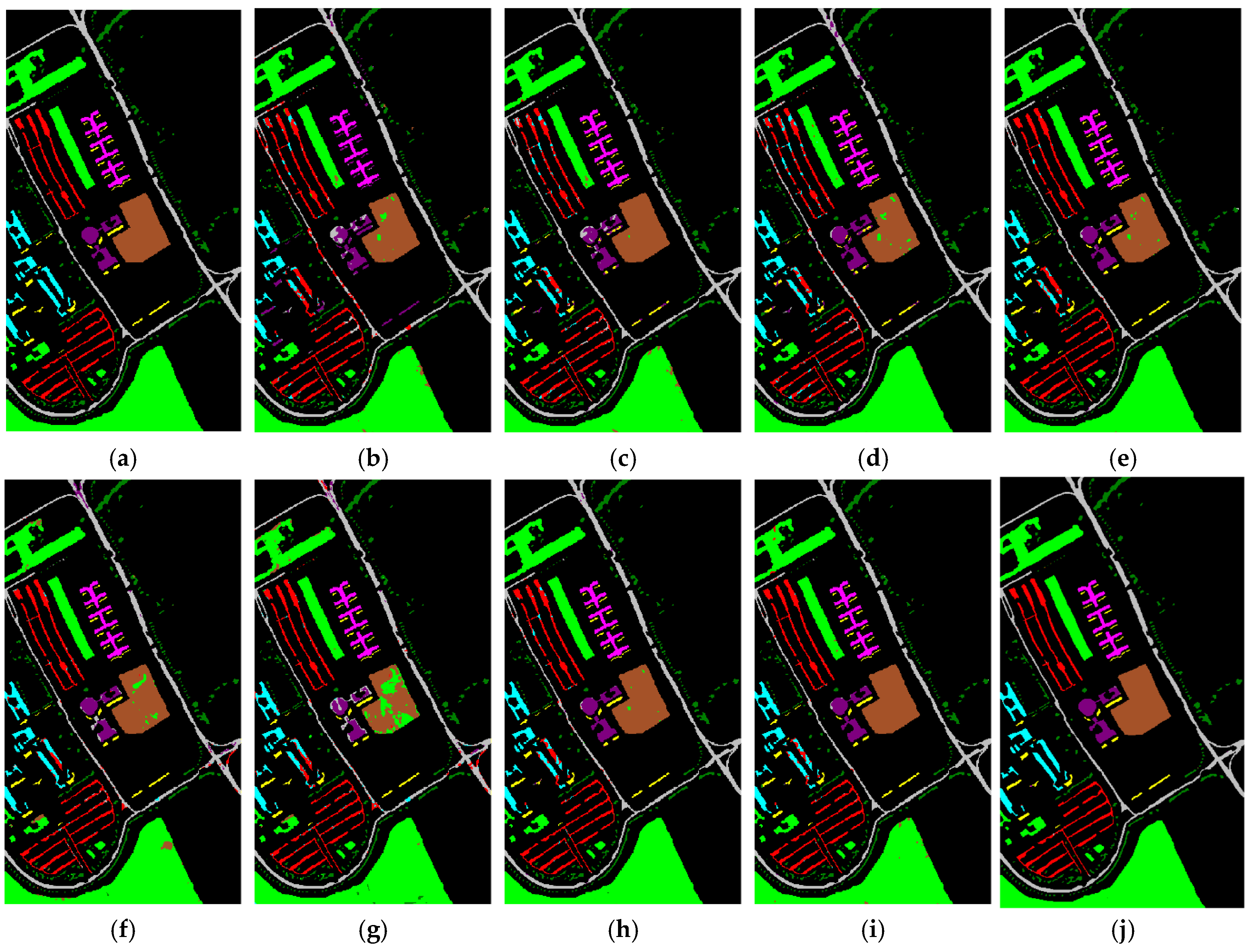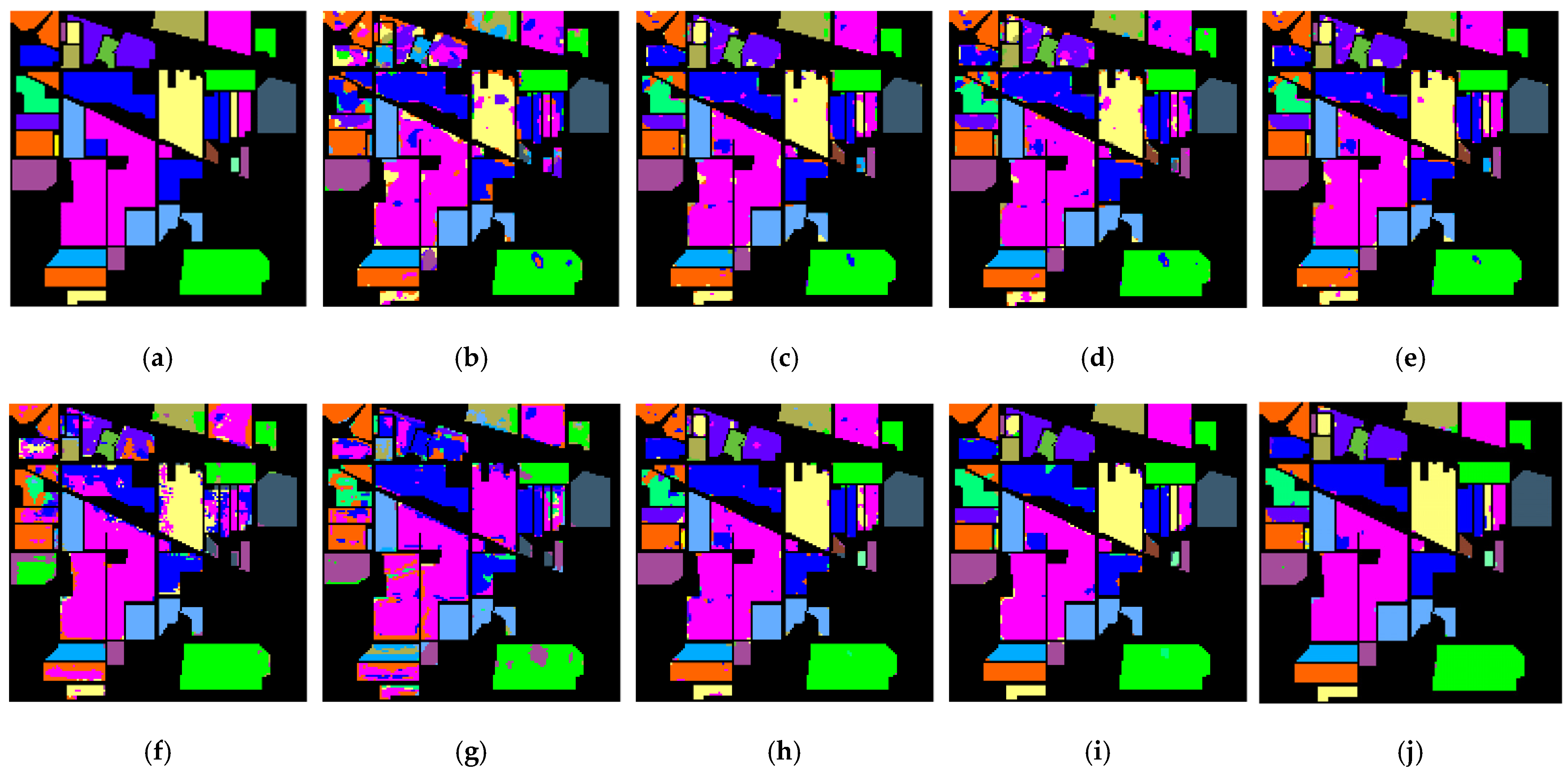Table 3, Table 4 and Table 5 correspond to the visualization label prediction graphs of experimental results, which are presented as Figure 13, Figure 14 and Figure 15 respectively.

The proposed DFAST method achieved AA% values of 99.94, 99.42, and 96.51 on the Salinas, Pavia University, and Indian Pines datasets, respectively, while morphFormer achieved AA% values of 99.75, 97.93, and 92.87, showing improvements of 0.19, 1.49, and 3.64, respectively. The proposed method achieved higher classification accuracy than all the compared graph neural network approaches.

In terms of the Kappa coefficient (multiplied by 100), DFAST achieved values of 99.95, 99.71, and 98.04 on the three datasets, compared to 99.78, 98.28, and 96.97 for morphFormer, with improvements of 0.17, 1.43, and 1.07, respectively. These results demonstrate that the proposed DFAST hyperspectral classification method consistently outperforms existing CNN and Transformer-based methods in terms of classification accuracy on the Salinas, Pavia University, and Indian Pines datasets.

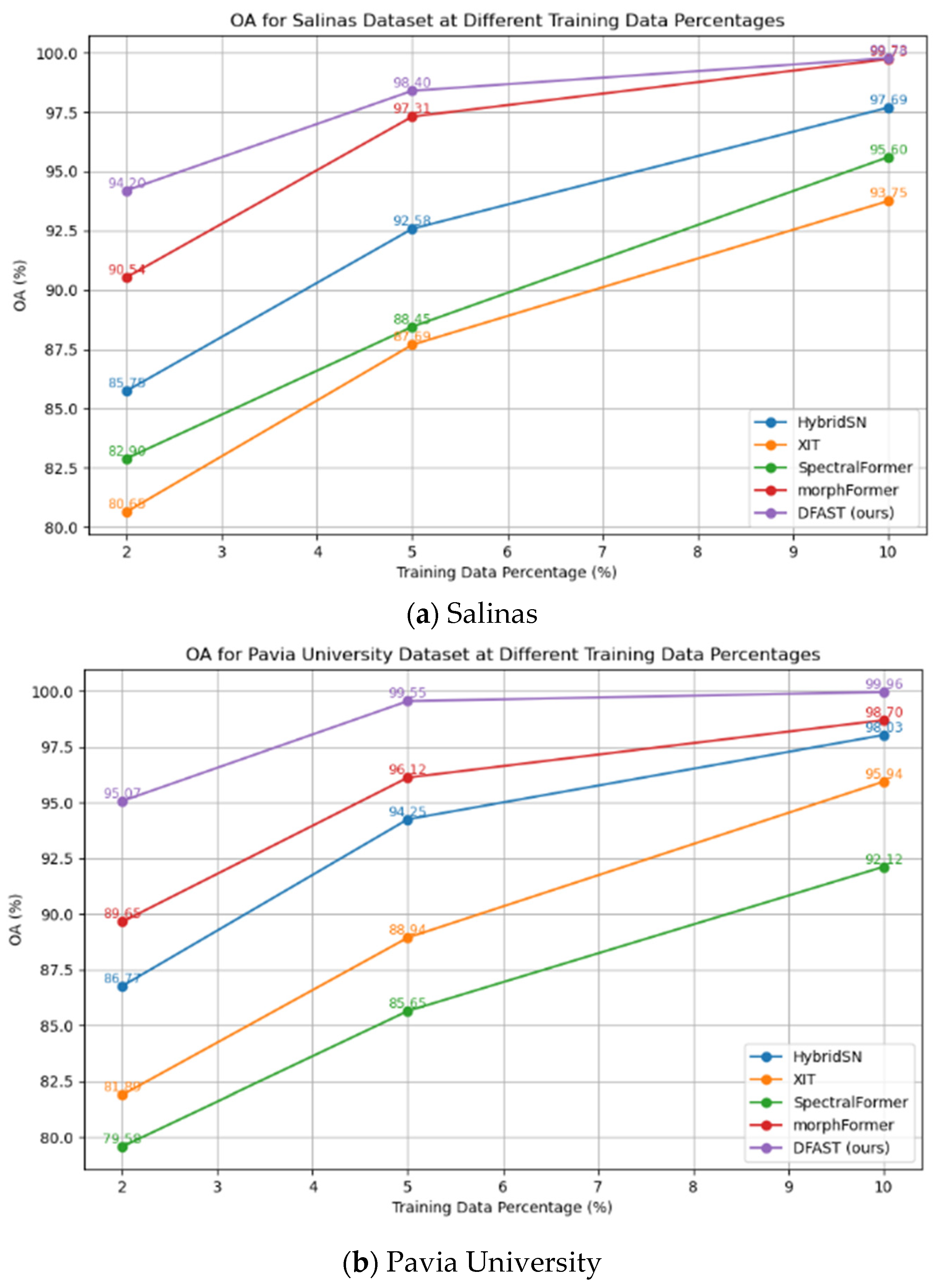
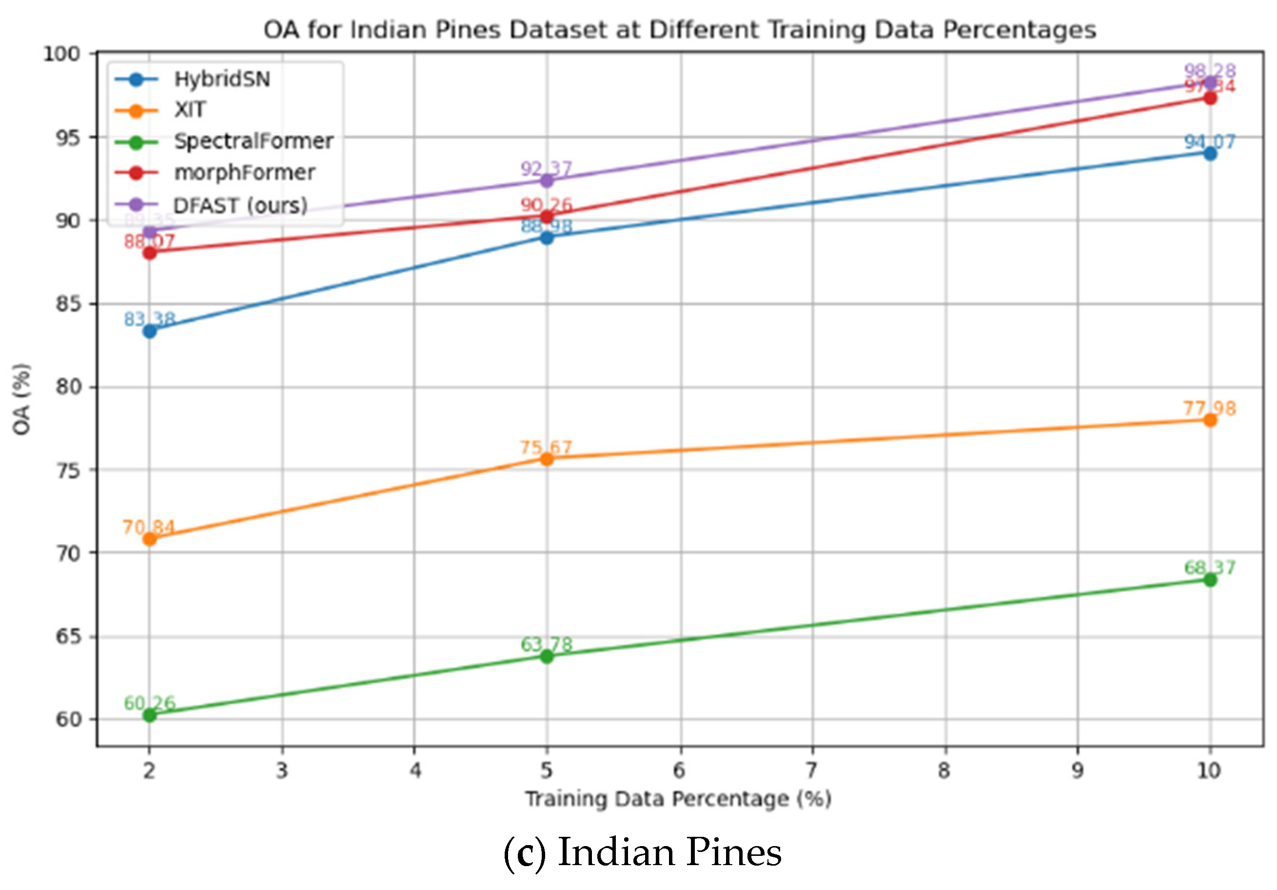
To evaluate the network’s classification performance under small-sample scenarios, we designed experiments to test the network’s accuracy when only 2%, 5%, and 10% of the data were used for training. The Salinas dataset contains 54,129 labeled samples, the Pavia University dataset contains 42,776 labeled samples, and the Indian Pines dataset contains 10,249 labeled samples. The experimental result curve is presented in Figure 16.

From the above results, it can be seen that even when only 2% of the data is used for training, the network achieves recognition accuracies of 95.07%, 94.20%, and 89.35% on the Salinas, Pavia University, and Indian Pines datasets, respectively, using 1082, 855, and 240 training samples. Compared with the best-performing morphFormer method under the same conditions (90.54%, 89.65%, and 88.07% on the three datasets), DFAST shows improvements of 4.53%, 4.55%, and 1.28%, respectively. This demonstrates that the proposed DFAST method significantly outperforms other networks when training data is limited.

4.6. Ablation Study

To verify the importance of the proposed DFAST band selection for classification, an ablation study was conducted as outlined in the table below. The study focused on three configurations: (1) raw spectral input, (2) differential-frequency domain features, and (3) the HSIChannelAttention module used for band selection. In the ablation study, only 2% of the Salinas and Pavia University datasets and 5% of the Indian Pines dataset were used for training. The model was trained for 100 epochs with the same experimental settings as before, and the results are summarized in

Table 7. Accuracy of the network on different datasets using different modules.

Raw Spectral	Differential-Frequency	HSIChannel Attention	Salinas (2%)			Pavia University (2%)			Indian Pines (5%)
			OA (%)	AA (%)	Kappa (%)	OA (%)	AA (%)	Kappa (%)	OA (%)	AA (%)	Kappa (%)
√	×	×	88.17	88.12	86.81	73.33	59.31	63.54	82.20	68.28	79.56
√	×	√	85.16	85.97	83.51	84.28	82.25	78.84	84.39	77.46	82.14
√	√	×	88.75	87.79	87.44	83.87	75.53	78.27	86.82	78.17	84.91
√	√	√	95.07	95.87	94.51	87.38	85.39	83.36	89.37	81.91	87.86

√ indicates ‘in use’ while × indicates ‘not in use’ for this module.

.

The data from Table 7 reveals that classification performance is relatively low when only raw spectral input is used (without differential and frequency domain features). Adding differential-frequency domain features significantly improves classification performance. For instance, in the Pavia University dataset, the OA% increases from 73.33% (raw spectral input) to 83.97% (with differential-frequency domain features). Furthermore, incorporating the HSIChannelAttention module further optimizes classification accuracy. For example, in the Salinas dataset, the OA% increases from 88.17% to 95.07%.

The addition of differential-frequency domain features effectively enhances the network’s ability to express spectral characteristics, while the inclusion of the HSIChannelAttention module adaptively selects important bands, further improving classification performance. Overall, the optimal configuration (raw spectral input + differential-frequency domain features + HSIChannelAttention) significantly outperforms other configurations, highlighting the critical importance of the combined use of these modules for classification performance enhancement.

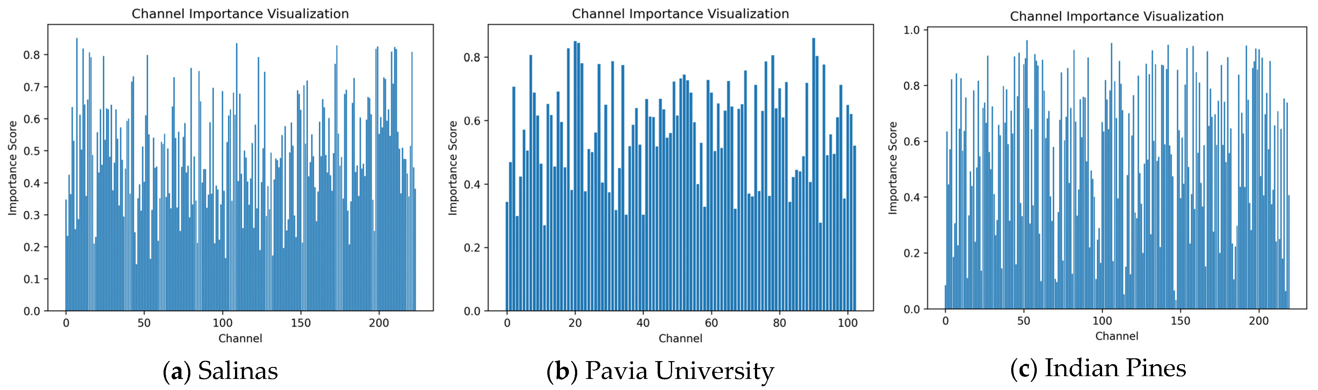
The trained classification network can also output the importance weight coefficients for each hyperspectral band, which can be used for dimensionality reduction. The weight coefficients for the Salinas, Pavia University, and Indian Pines datasets are shown in Figure 17.

The learned band weights proposed in the paper do not directly correspond to physical spectral properties. Instead, these weights represent the importance of spectral features within each channel for classification, thereby guiding the retention of spectral bands with higher weights during dimensionality reduction while preserving their physical significance.

Using the weight coefficients, the top 30 bands with the highest weights are selected to perform dimensionality reduction on the hyperspectral data. After dimensionality reduction, the HSIChannelAttention module used for band selection in the network is removed. This results in three configurations: ① raw spectral data, ② data reduced to 30 bands based on channel importance, and ③ data with 30 randomly selected bands. The training used 10% of the data for 300 epochs. The comparison of classification accuracies is shown in

Table 8. Classification accuracy after training with different band selections on three datasets.

	Salinas			Pavia University			Indian Pines
	OA (%)	AA (%)	Kappa (%)	OA (%)	AA (%)	Kappa (%)	OA (%)	AA (%)	Kappa (%)
①	99.96	99.94	99.95	99.78	99.42	99.71	98.28	96.51	98.04
②	99.80	99.80	99.77	99.53	99.27	99.38	99.29	98.65	99.19
③	89.03	86.34	88.69	88.12	87.36	85.08	86.25	83.11	85.36

. It can be seen that the classification accuracy using the top 30 bands selected by weight is significantly higher than the accuracy obtained by randomly selecting 30 bands.

Table 9. Training and testing time required for a single run before and after reducing the data.

Data	Salinas		Pavia University		Indian Pines
Time(s)	Train	Test	Train	Test	Train	Test
Before	417.15	42.78	179.03	16.92	83.21	8.66
After	107.81	7.76	91.65	6.37	23.51	1.60

presents the training and testing time required for a single run before and after reducing the data to 30 bands based on channel importance. As shown in the table, both training and testing times are significantly reduced after dimensionality reduction. This indicates that the proposed band selection module not only effectively improves classification accuracy but also significantly enhances the efficiency of the network. The channel importance represent the importance of the spectral features under each channel for classification, allowing the retention of spectral bands with higher original weights and their physical significance during dimensionality reduction.

5. Conclusions

In this paper, we propose a DFAST to address the issues of insufficient spectral information utilization, spectral redundancy, and difficulty in modeling spectral–spatial feature coupling in existing methods. Experiments on three real-world datasets (Indian Pines, Pavia University, and Salinas) show that the proposed method outperforms traditional classification methods and state-of-the-art deep learning networks in terms of classification accuracy.

The proposed DFAST model, with its differential-frequency domain attention band selection module and SCEncoder, effectively captures the global coupling relationships between spectral and spatial features. By combining 3D convolution, spectral–spatial attention mechanisms, and learnable band selection attention weights, DFAST not only adaptively selects important spectral bands but also significantly reduces spectral redundancy, enhancing the model’s robustness to noise and generalization ability. Furthermore, the band selection weights generated during the classification process provide interpretable support for hyperspectral image dimensionality reduction.

Traditional methods (e.g., SVM, 3D-CNN) typically process data directly in the original spectral or spatial domain, making them susceptible to high-frequency noise interference and limiting their ability to capture feature variations across different frequency bands. DFAST addresses these issues by employing fast Fourier transform (FFT) to decompose spectral data into low-frequency (global features) and high-frequency (local details) components, separately computing attention weights for each. This approach more effectively suppresses noise while enhancing discriminative features.

Existing Transformer-based methods (e.g., SSFTT) often process spectral and spatial features independently, leading to feature decoupling problems. The SCEncoder in DFAST overcomes this limitation by combining 3D convolution (for extracting local spectral–spatial features) with self-attention mechanisms (for modeling global dependencies), thereby achieving tighter spectral–spatial coupling.

Traditional band selection methods rely on manually designed criteria, whereas DFAST dynamically selects important bands through learnable attention weights. Additionally, it provides visualizable weight maps to improve interpretability of the decision-making process.

However, the current approach has some limitations:

When training samples account for less than 2% of the data, DFAST’s accuracy on complex categories drops by 5–10%, as the attention mechanism requires sufficient samples to learn effective weights. This could be mitigated by incorporating meta-learning techniques.

The computational cost of FFT remains relatively high. Future optimizations may include approximate Fourier transform methods (e.g., FFT pruning).

The automatic band selection may overly prioritize high-variance regions while neglecting low-variance but highly discriminative bands (e.g., certain vegetation indices). Introducing human-designed constraints (e.g., protecting NDVI-sensitive bands) could serve as a potential solution.

In the future, we will focus on exploring the global and local collaborative mechanisms in Transformer networks for spectral and spatial feature modeling and investigate more lightweight network structures to improve computational efficiency. Additionally, we will expand DFAST to applications such as small-sample classification and multimodal data fusion to further validate its generalizability and practical application value in hyperspectral remote sensing.