Article

A Cloud Vertical Structure Optimization Algorithm Combining FY-4A and DSCOVR Satellite Data

1
School of Remote Sensing and Information Engineering, Wuhan University, Wuhan 430079, China
2
Hubei Luojia Laboratory, Wuhan University, Wuhan 430079, China
3
Perception and Effectiveness Assessment for Carbon-Neutrality Efforts, Engineering Research Center of Ministry of Education, Institute for Carbon Neutrality, Wuhan University, Wuhan 430072, China
*
Author to whom correspondence should be addressed.
Remote Sens. 2025, 17(14), 2484; https://doi.org/10.3390/rs17142484
Submission received: 27 May 2025 / Revised: 10 July 2025 / Accepted: 15 July 2025 / Published: 17 July 2025
(This article belongs to the Section Atmospheric Remote Sensing)

Abstract

Clouds are important for Earth’s energy budget and water cycles, and precisely characterizing their vertical structure is essential for understanding their impact. Although passive remote sensing offers broad coverage and high temporal resolution, sensor and algorithmic limitations impede the accurate depiction of cloud vertical profiles. To improve estimates of their key structural parameters, e.g., cloud top height (CTH) and cloud vertical extent (CVE), we propose a multi-source collaborative optimization algorithm. The algorithm synergizes the wide-coverage FY-4A (FengYun-4A) and DSCOVR (Deep Space Climate Observatory) cloud products with high-precision CloudSat vertical profile data and establishes LightGBM-based CTH/CVE optimization models. The models effectively reduce systematic errors in the FY-4A and DSCOVR cloud products, lowering the CTH Mean Absolute Error (MAE) to 1.8 km for multi-layer clouds, an improvement of 4–8 km over the original. The CVE MAEs for single- and multi-layer clouds are ~2.5 km. Some bias remains in complex cases, e.g., multi-layer thin clouds at low altitudes, and error tracing analysis suggests this may be related to cloud layer number misclassification. The proposed algorithm facilitates daytime near-hourly cloud retrievals over China and neighboring regions.

Graphical Abstract

1. Introduction

Clouds are important to the Earth’s energy budget and atmospheric water cycle, with their spatiotemporal distribution directly affecting the radiation balance and precipitation patterns [1,2]. The cloud vertical structure (CVS), particularly the cloud top height (CTH), is a key parameter for monitoring storm systems. Within a TC, an increase in the CTH of deep convective clouds typically reflects enhanced convective activity and a greater magnitude of latent heat release, which in turn promotes the TC’s development and intensification [3]. Meanwhile, the CVS modulates the precipitation process, as within deep convective systems, greater vertical development, which results in a higher CTH, is capable of producing more intense rainfall [4]. Therefore, precise large-scale detection of CTH/CBH is of great value in understanding water cycle dynamics and predicting extreme weather.
The CTH and cloud vertical extent (CVE) are typically derived from active or passive satellite observations. Active sensors (e.g., CloudSat) offer high precision but have limited coverage [5,6], while passive sensors (e.g., MODIS) provide broad coverage but greater uncertainty regarding the CVS [7]. Consequently, the dominant approach is to integrate both active and passive observations, often using machine learning (ML) to fuse the datasets and enhance retrieval accuracy. For example, recent studies have successfully improved CTH retrievals by using ML to relate high-precision data from CALIOP (on CALIPSO) with passive observations from MODIS [8] and Himawari-8 [9], yielding promising results.
Although ML has improved the accuracy of CTH retrievals, the models above based on a single satellite data source still face notable limitations. One major challenge is the inability to effectively correct systematic errors due to the difficulty for passive remote sensing to obtain the signals of the lower part of clouds. For example, Tan et al. [10] developed a multi-layer cloud detection algorithm using Himawari-8 AHI data, but the algorithm exhibited a misclassification rate of up to 30%, primarily due to limitations in radiative transfer modeling for complex multi-layer cloud structures. Studies have shown that integrating heterogeneous satellite observations with varying spectral response functions and spatial resolutions can establish an error compensation mechanism through machine learning [11]. This is physically grounded in the fact that sensor-specific errors are typically independent [12], enabling the more effective decoupling of instrumental biases from true atmospheric signals. As a result, multi-source data fusion not only enhances model generalization but also improves the depth and robustness of error correction.
This study develops a fusion algorithm based on the Light Gradient Boosting Machine (LightGBM) and using the FY-4A (Feng-Yun-4A) and DSCOVR (Deep Space Climate Observatory) cloud products. The principle is that the CTH exhibits the existing regular error patterns in the different remote sensing products. Therefore, based on a data-driven approach, the actual vertical structure of the cloud can be inferred from these patterns. The technical approach includes data matching and model architecture. Data matching focuses on selecting spatiotemporally matched samples from the FY-4A, DSCOVR, and CloudSat. Model architecture involves establishing three models for cloud layer classification and CTH/CVE regression. By combining measurements from FY-4A and DSCOVR and regarding CloudSat’s vertical profile data as the ground truth, the new models deliver continuous daytime near-hourly CTH/CVE estimations in the Asia-Pacific region.

2. Data

This study investigates cloud profiles where the uppermost layer is classified as either in a liquid or ice crystal phase, while explicitly excluding profiles with a mixed-phase top layer (the detailed justification for this decision is provided in Appendix A). Our analysis is based on a dataset from January to May 2019, a period selected for the continuous and concurrent availability of all necessary cloud products from FY-4A, DSCOVR, and CloudSat/CALIPSO.

2.1. FY-4A Products

Feng-Yun-4A (FY-4A) is China’s second-generation geostationary meteorological satellite located at 104.7°E in a geostationary orbit. It carries the advanced Geostationary Earth Radiation Imager (AGRI) with 14 spectral channels, including the thermal infrared bands of channels 11–14, which cover 10.3–13.5 μm. Its view covers one-third of the Earth’s surface with a spatial resolution of 4 km every 15 min, spanning latitudes from 80.56°N to 80.56°S and longitudes from 174.72°E to 24.12°W.
In this study, we use Level 2 cloud products provided by the National Satellite Meteorological Center (NSMC, http://www.nsmc.org.cn (accessed on 3 September 2024)), which include the cloud top height (CTH, h F ), cloud top temperature (CTT, t F ), cloud top pressure (CTP, p F ), cloud layer phase (CLP, φ F ), and cloud layer type (CLT, κ F ). The FY-4A CTH product adopts the CO2/Split-Window algorithm [6,9,13]. The Split-Window method applies observations from two infrared window bands (with central wavelengths of 10.8 μm and 12.0 μm), and the CO2 slicing method uses observations from the CO2 absorption band (with a central wavelength of 13.5 μm). These two techniques are combined to retrieve the cloud top height [14].

2.2. DSCOVR Products

The Deep Space Climate Observatory (DSCOVR) satellite, positioned in orbit at the Sun–Earth first Lagrange point, continually observes the entire Earth disk illuminated by the Sun, offering enhanced spatial coverage in high-latitude regions [15,16]. Its Earth Polychromatic Imaging Camera (EPIC) features 10 narrowband spectral channels, including 764 nm (Oxygen A band) and 687.75 nm (Oxygen B band). It aims to retrieve cloud parameters over the Sun-illuminated surface at a spatial resolution of approximately 8 km [7,17,18]. The observation frequency fluctuates during the year. The interval is approximately 66 min during the period from late April to early September, and extends to 108 min during other months.
In this study, we utilize the EPIC Version 03 cloud products released by NASA Earthdata (https://search.earthdata.nasa.gov (accessed on 5 September 2024)), which include cloud effective height (CEH, h A   a n d   h B ), pressure (CEP, p A   a n d   p B ), and temperature (CET, t A   a n d   t B ) based on the oxygen A/B bands, as well as cloud phase ( φ D ), optical thickness of a liquid and ice cloud ( τ L and τ I ), and view geometry such as the sensor zenith angle ( ϑ D ) and solar zenith angle ( θ D ). The satellite retrieves cloud properties by measuring solar radiation absorption characteristics in the oxygen A-band (760 nm) and B-band (687 nm) and processes these measurements with the Mixed Lambertian-Equivalent Reflectivity (MLER) model. The fundamental principle assumes the cloud top acts as a reflecting surface at a certain pressure level. Given that atmospheric oxygen concentration and absorption cross-sections are known, measuring oxygen absorption intensity enables the estimation of photon path lengths above clouds, from which cloud top height can be derived [19,20]. By measuring the oxygen absorption in the path above this surface, an effective cloud pressure and height can be derived. However, the operational algorithm simplifies the retrieval by ignoring photon penetration and scattering within the cloud, yielding what are defined as the CEP and CEH, rather than the true geometric top values. In this study, we utilize these effective quantities (CEH, CEP, and the associated CET), for ease of comparison, as the DSCOVR CTH, CTP, and CTT products for our analysis.

2.3. CloudSat/CALIPSO Products

CloudSat and CALIPSO (Cloud-Aerosol Lidar and Infrared Pathfinder Satellite Observations) operate in a 705 km Sun-synchronous orbit, crossing the equator at local time 13:30, and forming a collaborative observation system. CloudSat is equipped with a 94 GHz active cloud profiling radar (CPR), offering high sensitivity to cloud water content and the strong penetration of thick clouds [2]. CALIPSO carries the Cloud-Aerosol Lidar with Orthogonal Polarization (CALIOP), which operates at wavelengths of 532/1064 nm and uses reflectivity depolarization techniques to retrieve the vertical distribution and phase of clouds [21,22]. The lidar is sensitive to thin clouds and aerosols, making it highly capable of detecting thin clouds.
We utilize the CPR and the CALIOP 2B-CLDCLASS-LIDAR product, which has a vertical resolution of 480 m with an orbital period of 98.3 min, covering the 82°N-S latitude range [22,23]. A primary limitation of CALIOP is that its lidar signal is attenuated by optically thick clouds, often preventing the detection of underlying cloud structures. Conversely, the CPR has a relatively coarse vertical resolution and may miss the optically thin clouds such as cirrus, and may instead retrieve the height of an underlying, warmer cloud as the cloud system’s true cloud top height [21]. Furthermore, recent validation studies indicate that the synergistic use of these sensors does not necessarily improve cloud phase classification; the 2B-CLDCLASS-LIDAR product, for instance, exhibits a systematic bias by overestimating the frequency of mixed-phase clouds, likely through the misclassification of pure ice or liquid layers [24].
Despite known uncertainties in determining the precise phase and boundaries of clouds, the synergy between CPR and CALIOP greatly enhances the characterization of these properties, making it a standard validation benchmark in numerous studies [8,9,13]. We use the 2B-CLDCLASS-LIDAR product as the ground truth in this study, including cloud layer top height ( h C ), cloud layer base height ( b C ), number of layers ( n C ), and cloud phase ( φ C ). Additionally, to describe the vertical dimension of the clouds, we use the general term cloud vertical extent (CVE). The specific calculation of CVE depends on the cloud layering. For single-layer clouds, CVE is defined as cloud geometrical thickness (CGT), calculated as the difference between the cloud top and base height. For multi-layer systems, CVE is defined as the cloud system depth (CSD), which is the distance from the top of the highest layer to the base of the lowest layer, a parameter that better represents the total vertical range perceived by passive sensors.

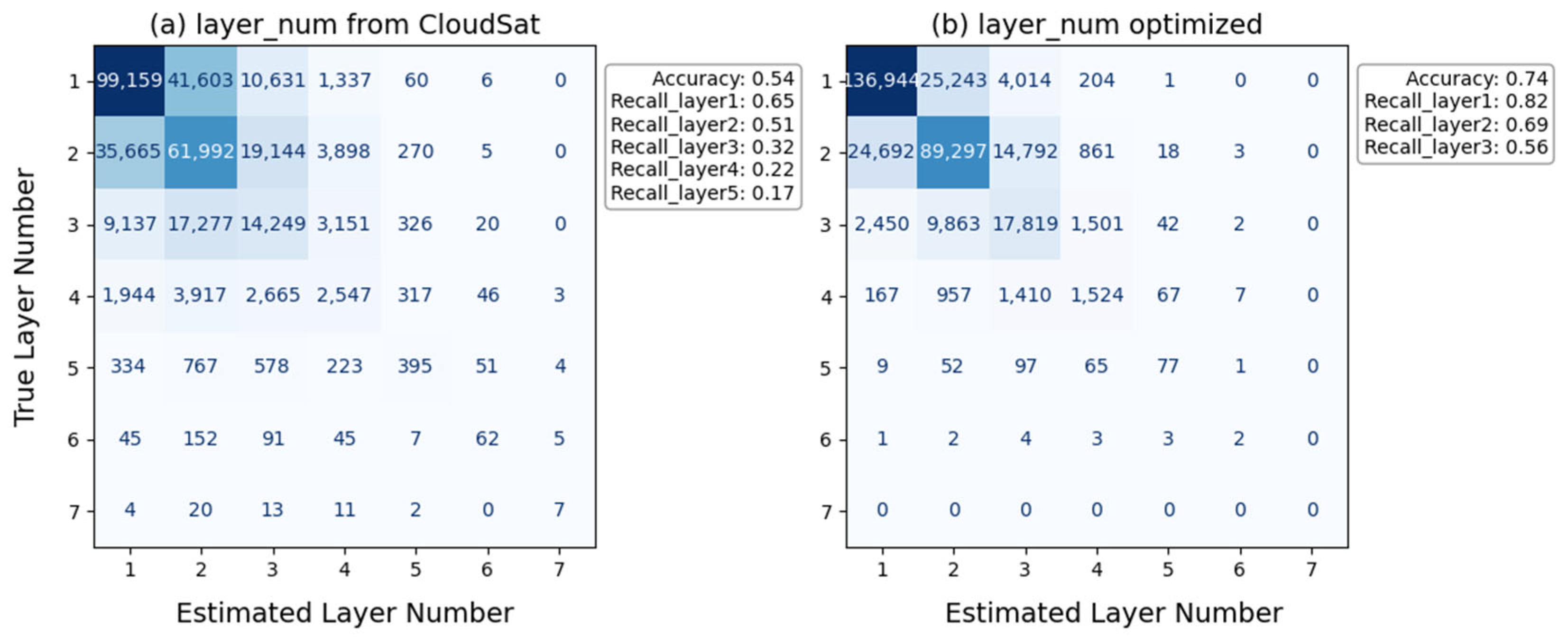
Adjustment of Cloud Layer Number

While the 2B-CLDCLASS-LIDAR product provides a precise layer count ( n C ), this fine-grained classification can create feature redundancy from the perspective of a passive sensor. Columns with varying layer counts might exhibit similar characteristics from the view of passive remote sensing; for example, two distinct, optically thin cirrus layers may be indistinguishable from a single, thicker one.
To create a training label more representative of such passive observations, we propose an adjustment based on physical similarity. This adjustment is defined by three criteria. First, the layers can be merged and must share the same cloud phase, as this indicates similar microphysical and radiative properties. Second, the vertical distance between them must be less than 1.5 km; radiative transfer within the intervening clear-sky gap cannot be considered negligible when the distance is large. Third, the thickness of any individual layer must be less than 3 km, which prevents the incorrect merging of separate, well-developed cloud systems. The resulting “adjusted cloud layer number” (CLN, n C ) is used as the ground-truth label in this study.
It is acknowledged that the CloudSat/CALIPSO product, while being the best available ground truth for global CVS studies, has its own uncertainties. A primary concern is the ~500 m physical vertical resolution of the CPR, which might lead to ambiguities in identifying closely spaced, thin cloud layers. However, this limitation must be evaluated in the context of the problem we aim to solve. Passive sensors, which this study seeks to optimize, are themselves insensitive to fine vertical structures; their effective vertical resolution for the underlying layers is significantly coarser than that of the active sensors. Our layer-merging approach is therefore a deliberate design choice, coarsening the “truth” classification to better match what a passive sensor can realistically discern. Judged against the observational capabilities of passive remote sensing, the ~500 m vertical resolution of the CloudSat/CALIPSO product is thus considered more than adequate for the purpose of training our optimization model.

2.4. Problems in Passive Remote Sensing

Passive remote sensing has its own systematic errors, stemming from the various principles by which sensors acquire information. Therefore, we utilize active remote sensing cloud products to assess the accuracy of passive remote sensing cloud products. Below are the systematic errors present in the passive remote sensing CTH products used in this study.

2.4.1. FY-4A CTH Systematic Error

The CTH retrieval for FY-4A is based on thermal infrared (TIR) radiative transfer theory. The core principle involves retrieving cloud top temperatures from the radiation difference between the 10.8 μm and 12.0 μm infrared window channels, and then calculating the CTH using the atmospheric temperature profile [14]. Its performance heavily relies on the characteristics of the cloud layer structure, as thermal emission from lower portions of the cloud or underlying layers can also contribute to the satellite-observed radiance.
Figure 1a presents the cloud top height (CTH) retrieval accuracy for single-layer cloud systems, demonstrating an RMSE of 3.9 km and MAE of 2.6 km. The data points collectively exhibit a systematic underestimation pattern, while most of them align reasonably well with the 1:1 reference line.
In contrast, the multi-layer cloud systems (Figure 1d) show significantly degraded retrieval accuracy, with RMSE increasing to 6.6 km and MAE to 5.4 km. This performance reduction stems from the known limitations of TIR-based retrievals when observing high, semi-transparent clouds. The underlying physical mechanism is that the passive sensor does not sense the true geometric top but effectively “sees into” the cloud to a certain optical depth [6]. This results in the received radiance being contaminated by warmer thermal emissions from within or below the cloud, leading to a retrieved CTH that is systematically biased to be low. This effect is particularly pronounced in multi-layer cloud systems, where studies consistently find that the retrieved CTH is often placed somewhere between the upper and lower cloud layers [13,25].
Figure 2 reveals a clear height-dependent bias in the CTH retrievals from all instruments. For low clouds (CTH < 4 km), the FY-4A retrievals show low bias, with the mean error (ME) consistently between −1 km and +1 km for both single- and multi-layer systems (yellow lines). However, as the cloud top height increases, a systematic underestimation bias becomes prominent. For clouds with a CTH above 4 km, the ME becomes progressively more negative, indicating that the retrieved height is increasingly lower than the true height. This underestimation is more severe for multi-layer clouds (solid yellow line) than for single-layer clouds (dashed yellow line). For instance, at 16 km, the underestimation for multi-layer clouds (ME ≈ −8 km) is significantly greater than that for single-layer clouds (ME ≈ −5 km).

2.4.2. DSCOVR CEH Discrepancy

Figure 1b,c compare the DSCOVR cloud effective height (CEH) against the CTH from CloudSat/CALIPSO for single-layer cloud systems (RMSE = 5.5/6.1 km, MAE = 4.2/4.7 km), showing a cluster in line as Figure 1a does, but with a lower slope, which indicates a larger discrepancy.
For the multi-layer cloud system shown in Figure 1e,f, the discrepancy becomes even more pronounced (RMSE = 9.4/10.1 km, MAE = 8.9/9.5 km), with points densely clustering in the lower right corner, indicating a greatly negative bias in the high-altitude interval.
Figure 2 reveals the height-dependent discrepancy between DSCOVR’s CEH and the reference CTH. The mean difference (ME) becomes increasingly negative with altitude, and this discrepancy is consistently larger for the B-band (red lines) than the A-band (blue lines), and is more pronounced for multi-layer (solid lines) versus single-layer (dashed lines) clouds. For high-altitude multi-layer systems, this culminates in a large ME, with values more negative than -10 km for both the A-band and B-band.
Key explanations for this phenomenon are provided by theoretical studies from Yang et al. [7], Davis et al. [17,18], and Marshak et al. [15]. The operational Mixed Lambertian-Equivalent Reflectivity (MLER) algorithm intentionally simplifies the radiative transfer problem by ignoring photon penetration and scattering within the cloud. This model deficiency results in a systematic negative bias in DSCOVR CEH retrievals for single- and multi-layer cloud systems. Notably, Yang et al. [26] further discovered that in multi-layer cloud systems, the complexity of the cloud structure and interactions between layers amplify this systematic bias. In Figure 1, the RMSE of the CEH retrievals for multi-layer clouds (9.4 km) is 71% higher than that of single-layer clouds (5.5 km), confirming the negative impact of vertical cloud structure complexity on retrieval accuracy.
The CTH products from FY-4A and DSCOVR satellites both exhibit distinctly linear point distributions for single-layer clouds, with their primary difference manifested in slope variations. In contrast, under multi-layer cloud conditions, their distribution characteristics show marked differences. FY-4A data points are predominantly clustered in the upper right corner near the 1:1 line, while DSCOVR data points concentrate densely in the lower right corner. The two products demonstrate fundamentally distinct discrepancy patterns between single-layer and multi-layer clouds. These layer-dependent patterns suggest that combining both satellite products may effectively identify the number of layers.

3. Methodology

3.1. Spatiotemporal Collocation

3.1.1. Matching for Model Training

To optimized the cloud heights from FY-4A and DSCOVR using the 2B-CLDCLASS-LIDAR CTH as ground truth, we established a multi-sensor dataset that was collocated in both space and time through the following strict screening criteria: (1) temporal collocation, which requires near-simultaneous satellite transits, and (2) spatial consistency, which requires co-located valid data from all three sensors within a defined geographic domain. The filtered pixels (FY-4A and DSCOVR) and soundings (CloudSat/CALIPSO) are recognized as temporally concurrent and spatially adjacent. Figure 3 illustrates the overlap of FY-4A, DSCOVR, and CloudSat/CALIPSO at several consecutive times.
A key challenge in fusing these datasets is the significant mismatch in their observational characteristics. The instruments operate on different schedules and spatial resolutions: FY-4A provides imagery with a spatial resolution of 4 km every 15 min; DSCOVR provides imagery with a spatial resolution of 8 km every 66 to 108 min, with the observations for the 10 wavelengths taken over a time span of 7 min; while CloudSat/CALIPSO offers fine-resolution (1.4 km) along-track soundings approximately every 98 min. Due to this lack of spatiotemporal synchronization, exact co-locations are rare. Consequently, this study suggests a spatiotemporal proximate matching strategy, outlined as follows:
1.
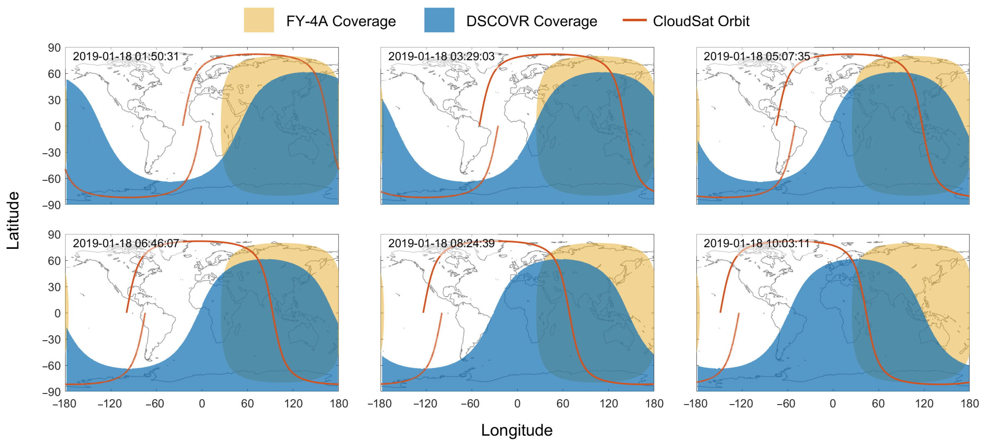
Temporal Pre-Screening: FY-4A and DSCOVR images are selected based on their imaging times and CloudSat/CALIPSO’s flight plan. One CloudSat/CALIPSO orbit may correspond to multiple FY-4A images. This is because, when CloudSat/CALIPSO passes through the sunlit side of the Earth, FY-4A captures images many times with a much higher frequency than that of CloudSat/CALIPSO.
2.
Spatial Matching: Given the large number of pixels in the images, global brute-force matching is time-consuming. Therefore, we employ a two-step method to improve the matching efficiency. First, for each CloudSat/CALIPSO sounding, we define a 3° × 3° bounding box (approximately 1.5° in each direction) and discard all FY-4A and DSCOVR pixels falling outside this area. Second, we calculate the geodesic distance from each of these candidate pixels in the box to the sounding using the Haversine formula [27]. The closest pixel is then identified, and to ensure high spatial consistency, the geodesic distance from the matched FY-4A and DSCOVR pixels to the sounding should be less than 5 km.
3.
Temporal Matching: A temporal matching is carried out at the pixel level. If the time difference between the matched FY-4A and DSCOVR pixels and the CloudSat/CALIPSO sounding is less than 15 min, they are considered to have been captured within the adjacent time frame. The 15 min threshold is chosen as a compromise between dataset size and physical consistency. A stricter window (< 5 min) was found to discard over 80% of potential matches. Conversely, a longer window is physically questionable, as the cloud properties from a fixed-point perspective significantly decorrelate on a timescale of about 15.5 min [28]. Furthermore, the 15 min window is designed to accommodate occasional 30 min gaps in the FY-4A data stream, ensuring better data matching.

3.1.2. Matching for Model Application

In the model application phase, we have to perform spatiotemporal matching of the FY-4A and DSCOVR cloud products and apply the model to the matched data to optimize the CTH/CVE in the overlapping areas of the FY-4A and DSCOVR cloud products. The matching method is similar to that in Section 3.1.1. Since the DSCOVR cloud product has a lower spatial resolution, we center the matching process on DSCOVR pixels and find the spatiotemporally closest FY-4A pixels.

3.2. CTH/CVE Optimization

The different error distributions of FY-4A and DSCOVR in Figure 1, along with the strong correlation between their errors and cloud height in Figure 2, suggest that the differences between these cloud products can reflect different types of cloud systems and even indicate their deviations from the actual cloud top height. Following this line of thought, we present an algorithm made up of three models: the cloud layer number (CLN) model, designed to identify single-layer and multi-layer cloud systems; the cloud top height (CTH) model, which directly optimizes the cloud top height; and the cloud vertical extent (CVE) model, which is for indirectly calculating the cloud base height.

3.2.1. Dataset Splitting

A total of 332,194 cloudy pixels were collected and divided into two groups with a 1:4 ratio. The first group was used for the CLN model, while the second was for the CTH/CVE model. For each dataset, we split it into training, validation, and test sets in an 8:1:1 ratio again and trained the three models mentioned individually.

3.2.2. CLN Estimation Model

In this study, to address the challenges of CTH retrievals in multi-layer cloud systems (refer to Section 2.4), we plan to use the CLN as the input for the CTH/CVE model. However, since FY-4A and DSCOVR cloud products do not supply the number of cloud layers, it is crucial first to establish a CLN estimation model based on the differing sensitivities in CLN between FY-4A and DSCOVR, and to train it using the adjusted cloud layer number ( n C ) determined with CloudSat/CALIPSO. This model can then provide the estimated cloud layer number ( n M ) over large areas and assist in estimating CTH and CVE. The data list for model training is displayed in Table 1.

3.2.3. CTH/CVE Optimization Model
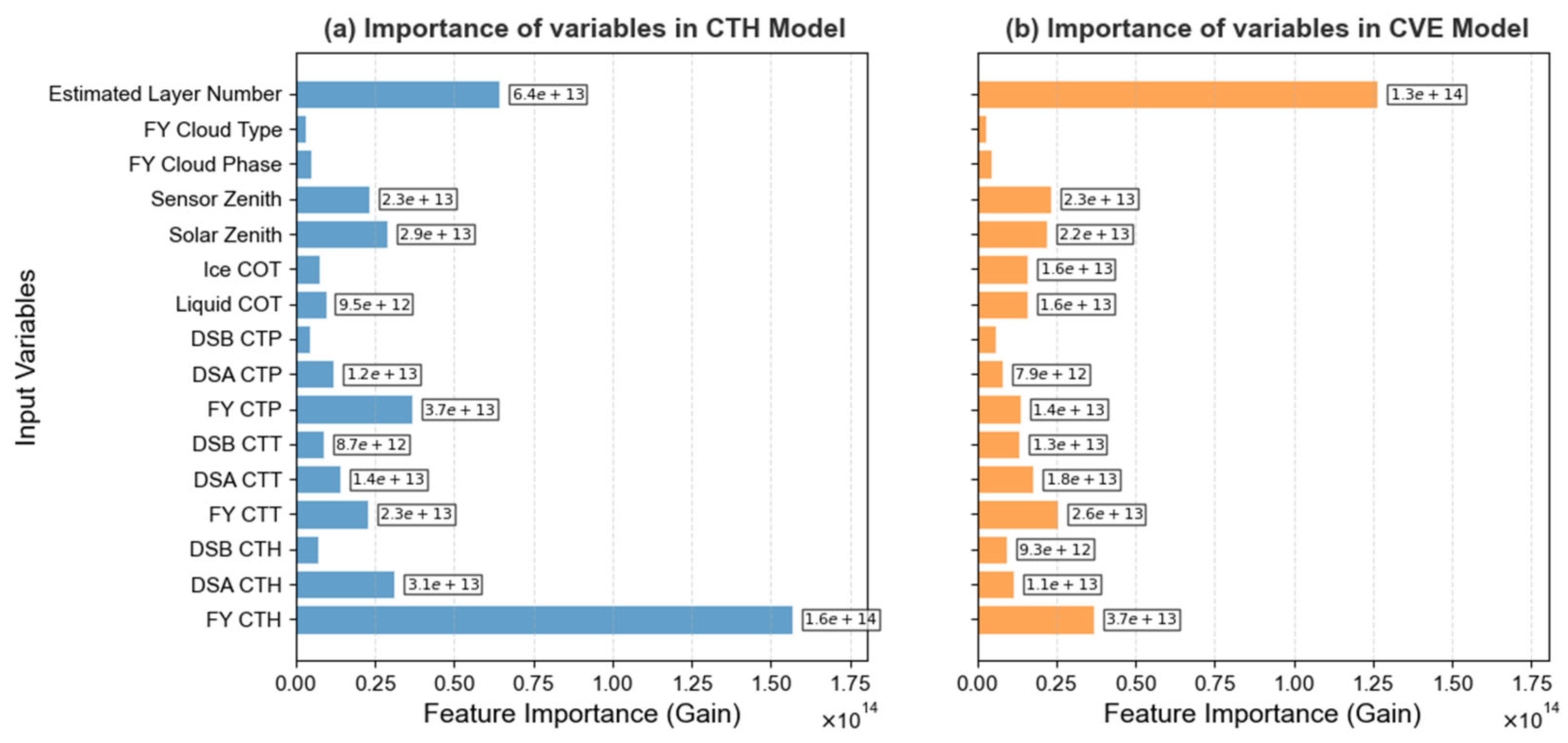
The cloud top height (CTH) model and the cloud vertical extent (CVE) model are trained separately, using the same input. The input variables for the CTH/CVE model are set as follows:
1.
Cloud Parameters: These include the cloud top height ( h F ), temperature ( t F ), and pressure ( p F ) from the AGRI/FY-4A products, along with those retrieved from the oxygen A/B absorption bands of EPIC/DSCOVR ( h A , t A , p A , h B , t B , p B ). Additionally, the cloud layer phase ( φ F ) and type ( κ F ) from FY-4A, as well as the liquid and ice cloud optical thickness ( τ L , τ I ) from DSCOVR are selected as input variables.
2.
View Geometry: Changes in the solar zenith angle ( θ D ) can affect the depth of photon penetration into the cloud layers and the length of the transmission path [3,29]. This geometric effect directly leads to systematic biases in the retrieval of CTH based on the O2-A/B absorption bands (as discussed in Section 2.4.2). Additionally, an increase in the sensor zenith angle ( ϑ D ) can alter the cloud top radiation characteristics [13]. The model incorporates both angle parameters as key radiation transfer constraint variables.
3.
Cloud Layer Number: The number of cloud layers distinguishes between single- and multi-layer clouds. We include the estimation of cloud layer number, as discussed in Section 3.2.2, as an input variable.

3.2.4. Model Training

The model development, data analysis, and visualization for this study were performed using Python (version 3.12) and MATLAB (version R2023a). The core optimization models were developed using the LightGBM algorithm (version 4.6.0) [30] based on the Gradient Boosting Decision Tree (GBDT) framework. LightGBM’s leaf-wise growth strategy prioritizes splitting the leaf node that yields the great reduction in loss, demonstrating superior computational efficiency and predictive accuracy in regression tasks [31,32]. This feature makes LightGBM particularly well-suited for managing high-dimensional remote sensing datasets derived from multi-source satellites like FY-4A and DSCOVR.
For the CLN classification model, we used the multi-class cross-entropy loss (MCEL) as the evaluation metric, while the Root Mean Squared Error (RMSE) was used for the CTH/CVE regression models. Through a series of tuning experiments, an optimal learning rate of 0.005 was identified for all models, which provided a good balance between convergence speed and final accuracy. The complete, final hyperparameter configurations for each model, which were determined through multiple tests, are summarized in Table 2.
To further enhance the algorithm’s robustness, a dynamic early stopping strategy and a double random sampling mechanism are integrated for the CLN, CTH, and CVE models. Specifically, the model training automatically terminates if the evaluation metric does not improve for 50 consecutive rounds. This helps balance the model’s convergence efficiency and the risk of overfitting. Additionally, in the feature dimension, only 75% of the features are randomly selected for node splitting in each iteration, reducing the model’s sensitivity to noisy features by suppressing feature collinearity [33]. In the sample dimension, Bootstrap sampling is performed every four iterations, randomly selecting 75% of the training samples to update the data distribution. This forces the model to optimize on differentiated data subsets continuously, enhancing the diversity of the gradient update directions. Experiments showed that, compared to traditional GBDT strategies, the double random sampling strategy reduced the RMSE on the validation set by 5.5%.

3.3. Evaluation Methods

This study uses the RMSE (Root Mean Squared Error), MAE (Mean Absolute Error), and R2 (coefficient of determination) as evaluation metrics for the CTH and CVE optimization, and the accuracy (α) and recall rate ( ρ i ) for the CLN estimation. In Equations (1) and (2), n i , j represents the number of samples that actually have i layers and are determined to have j layers. RMSE measures the model’s estimation ability. MAE is robust to outliers and is more stable than RMSE. The smaller the RMSE or MAE, the more accurate the model’s predictions. R2 represents the proportion of the total variance that the model explains. It measures the degree to which the model fits the data. The value ranges from 0 to 1, and the closer the value is to 1, the stronger the model’s explanatory power.
α = i n i , i i j n i , j
ρ i = n i , i j n i , j

4. Results

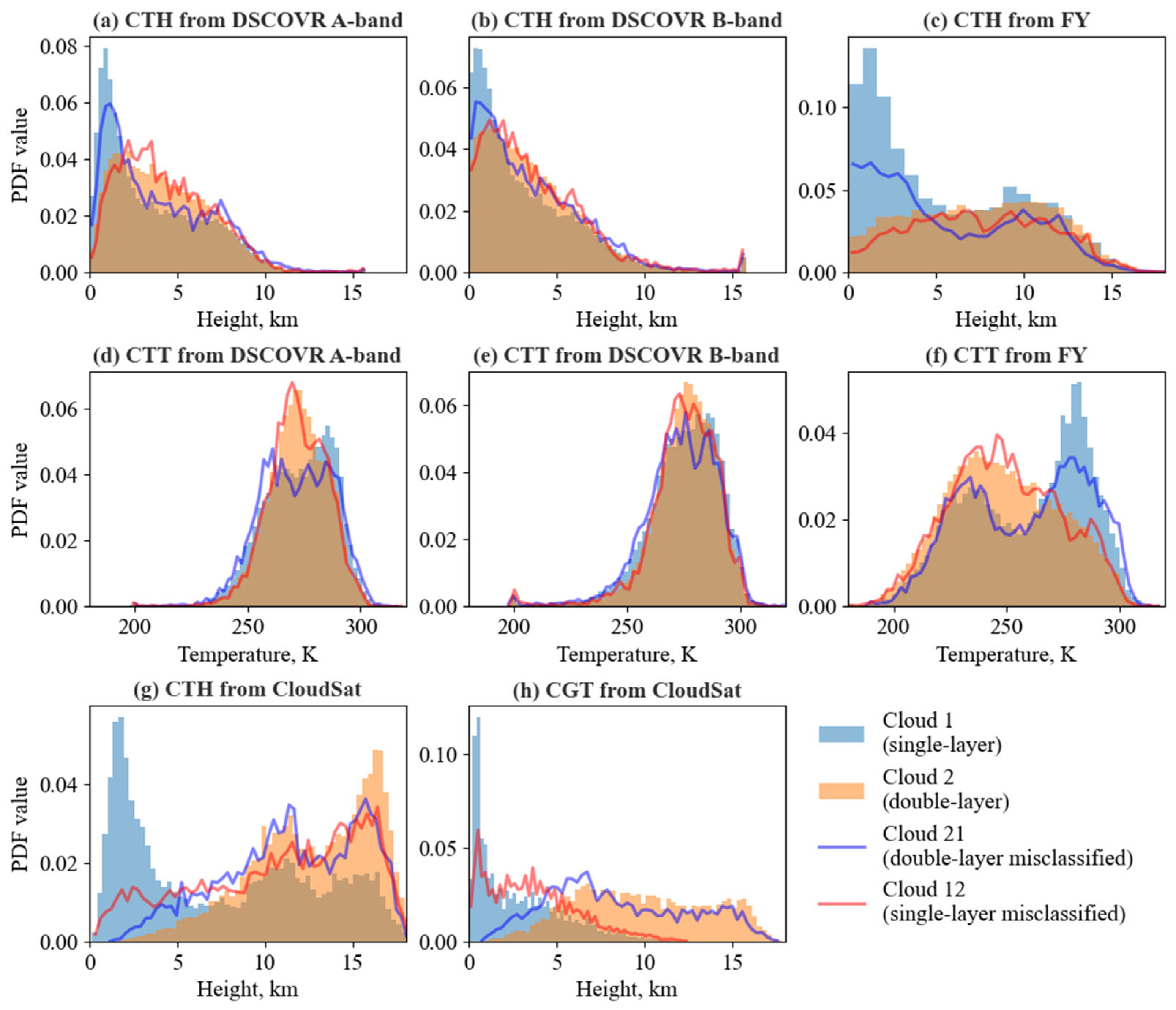
4.1. CLN Model Performance

In the CLN model training, we utilized the adjusted number of clouds ( n C ) rather than the original ( n C ) as the training label. Figure 4a,b illustrate the accuracy of CLN models trained using the cloud layer number before and after adjustment.
The adjustment shows the benefits we expected. Firstly, the adjusted model achieves an overall accuracy of 74%, representing a 20% improvement over the original model. Secondly, the adjusted model has enhanced multi-layer cloud identification. For clouds with two and three layers, the recall rates reach 69% and 56%, respectively, marking improvements of 18% and 24% compared to the original. Finally, the adjustment improves consistency in identifying multi-layer cloud systems. The original 2B-CLDCLASS-LIDAR dataset contains numerous high-complexity cloud samples with more than three layers, accounting for about 7% of the total samples. The recall rates for the samples with four and five layers in Figure 4a are as low as 22% and 17%, respectively. After the adjustment, the proportion of multi-layer cloud samples with more than three layers is reduced to 2%, minimizing redundant features.
Figure 4b also shows that a few single-layer clouds are still incorrectly identified as multi-layer clouds and vice versa. For instance, 19% of double-layer clouds are misclassified as single-layer clouds, while 15% of single-layer clouds are misclassified as double-layer clouds. These misclassified samples would introduce systematic biases in the subsequent CTH/CVE model training.

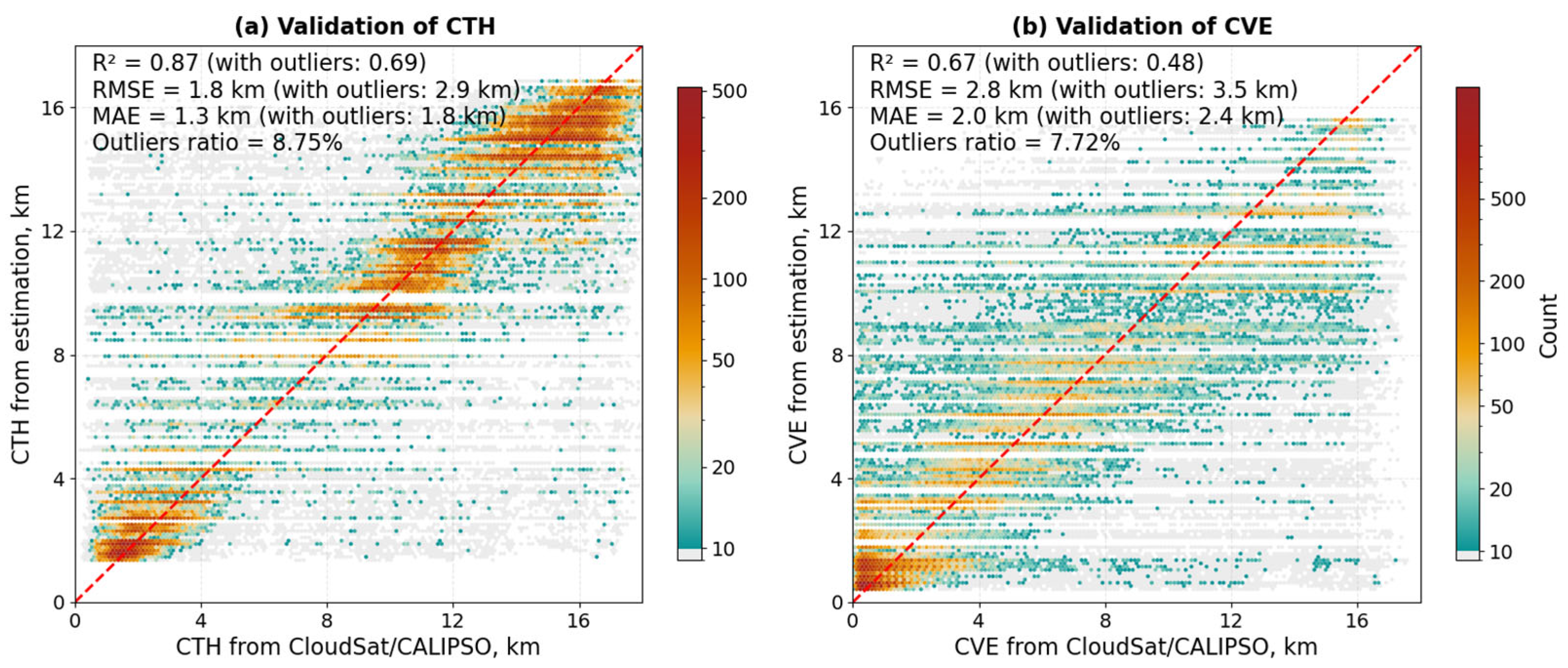
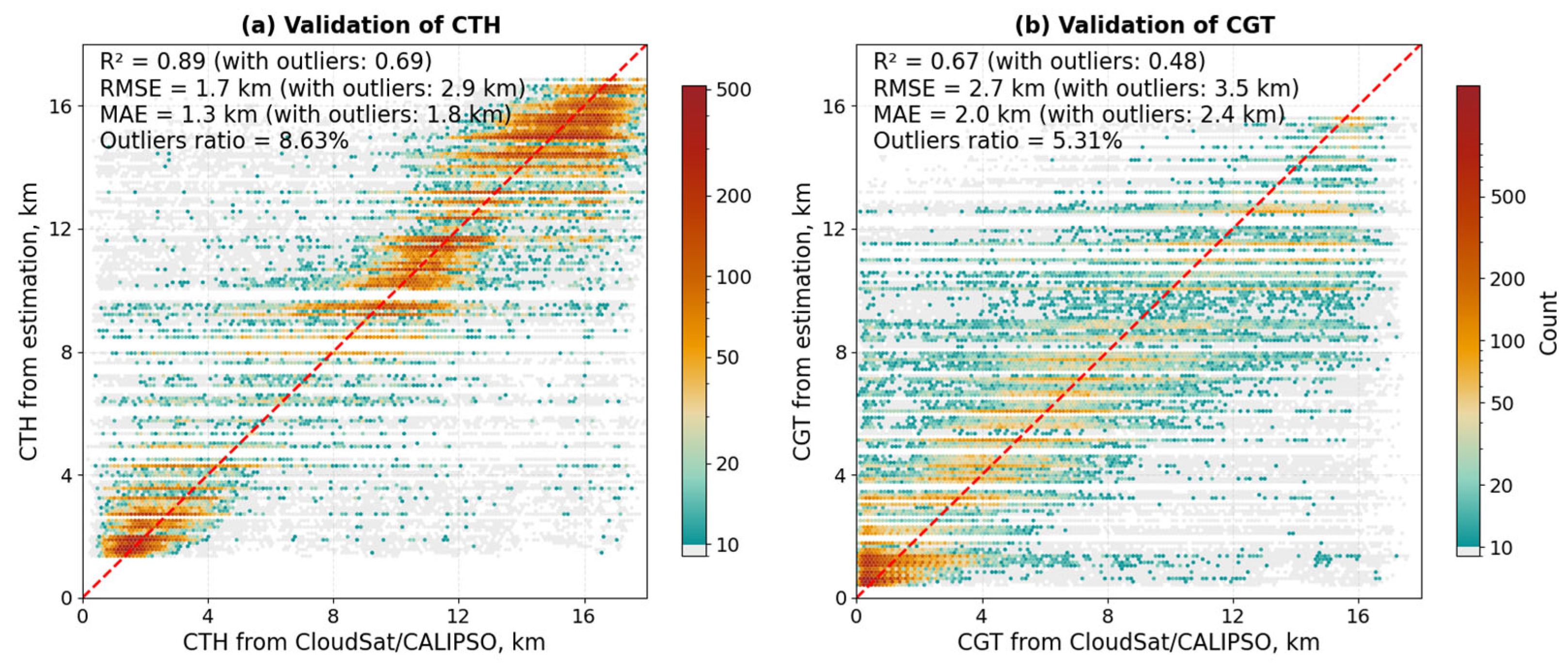
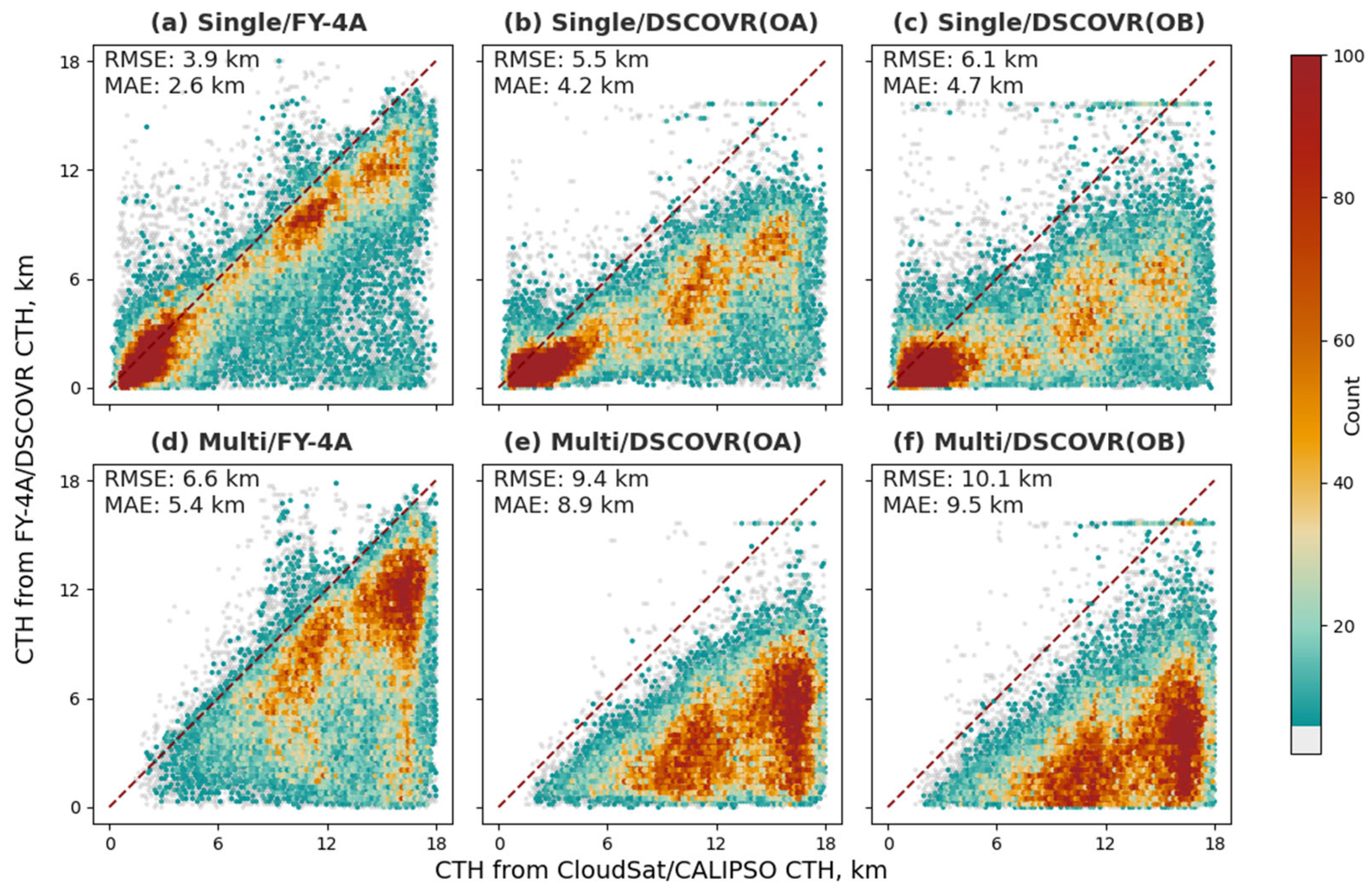
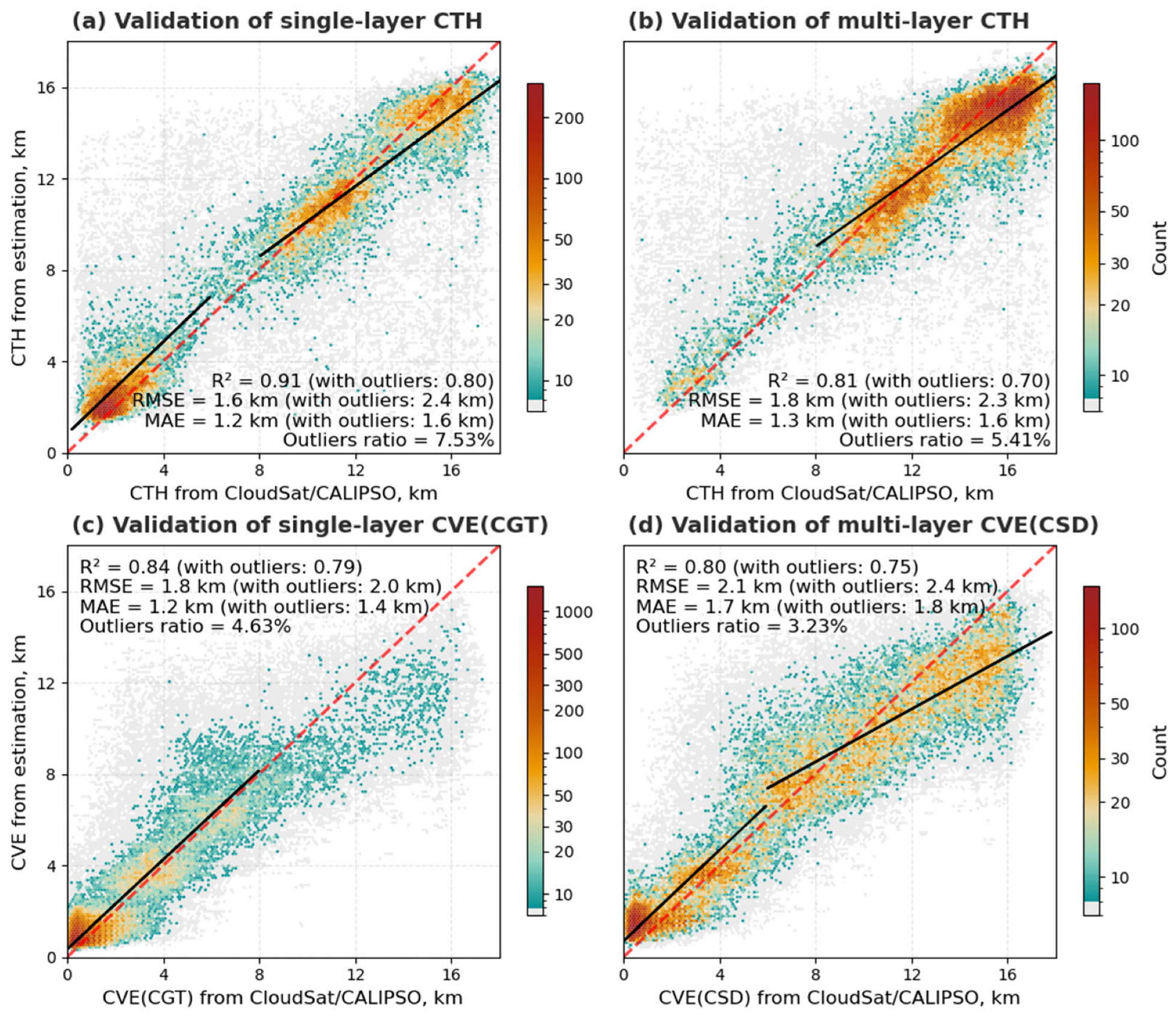
4.2. CTH/CVE Model Performance

The CTH/CVE optimization model proposed in this study demonstrates good performance on the test set. Figure 5a demonstrates that the CTH model achieves superior performance with an RMSE of 2.8 km, an MAE of 1.9 km, and an R2 of 0.70. After excluding outliers, the RMSE and MAE decrease to 2.0 km and 1.5 km, respectively, and the R2 increases to 0.84. In the lower part (CTH < 6 km) of Figure 5a, the slope of the fitted line is close to the 1:1 line but the intercept is about 2 km. For the higher part (CTH ≥ 8 km), the fitted line is closer to the 1:1 line, revealing better accuracy for high clouds.
Outliers were identified using the Interquartile Range (IQR) method, which classifies a data point as an outlier if its prediction error—calculated as the difference from the CloudSat/CALIPSO ground truth—falls by more than 1.5 times the IQR below the first quartile (Q1) or above the third quartile (Q3) [34].
Figure 5b presents the accuracy of the CVE (cloud geometrical thickness (CGT) for single-layer clouds, cloud system depth (CSD) for multi-layer clouds) model, with an RMSE of 3.5 km, MAE of 2.6 km, and R2 of 0.50. After excluding outliers, the RMSE and MAE decrease to 3.0 km and 2.3 km, respectively, and the R2 increases to 0.62. In the thinner part (CVE < 6 km), points cluster at 1–4 km above the 1:1 line. Meanwhile, for the thicker part (CVE ≥ 6 km), the fitted line slope decreases significantly, revealing a systematic underestimation and suggesting the model’s limitations in capturing thick clouds.
The evaluation metrics for removing outliers are only used in the above two paragraphs. The evaluation metrics containing outliers are used in all subsequent paragraphs and are summarized in Table 3.
(A)
Performance in Single-Layer Clouds
Based on the estimated CLN, we categorize the samples used in Figure 5 into single- and multi-layer cloud systems. Figure 6a demonstrates the CTH’s accuracy in single-layer cloud systems, achieving an R2 of 0.69, an RMSE of 3.0 km, and an MAE of 2.0 km, which is improved beyond the FY-4A (RMSE = 3.9 km, MAE = 2.6 km) and the DSCOVR (RMSE = 5.5 km, MAE = 4.2 km). The single-layer cloud test set contains 8.09% outliers, and their removal leads to 30% and 25% improvements in RMSE and MAE, respectively. Specifically referring to the part below 6 km in Figure 6a, the points cluster above the 1:1 line, showing a systematic overestimation of 1–2 km. Within the height ranges of 9–12 km and 13–17 km, the points closely align with the 1:1 line, demonstrating the model’s good accuracy in single-layer clouds with high cloud tops.
Figure 7a shows the MAE of CTH calculated in each 1 km height bin for single- and multi-layer clouds. For single-layer clouds (the dark blue line), the MAEs are generally under 2 km and the calculation performs particularly well in the densely sampled 1–4 km range, where the MAE is consistently around 1 km. Slightly higher MAEs (>2 km) are observed in the 0–1 km, 4–7 km, and 16–18 km ranges, which correspond to regions with relatively fewer samples.
Figure 6c shows the CVE model’s performance under single-layer cloud conditions, yielding an R2 of 0.43, an RMSE of 3.3 km, and an MAE of 2.3 km. Notably, although the MAE of single-layer clouds in Figure 7b rises intensely along with the increasing vertical extent (the red line), thick cloud samples account for a relatively small proportion in the dataset (the red histogram in Figure 7b), thus the impact on operational applications remains relatively minor.
(B)
Performance in Multi-Layer Clouds
Figure 6b shows CTH optimization in multi-layer systems, achieving an R2 of 0.60, an RMSE of 2.7 km, and an MAE of 1.8 km, which represent a substantial improvement over FY-4A (RMSE = 6.6 km, MAE = 5.4 km) and DSCOVR (RMSE = 9.4 km, MAE = 8.9 km). The clouds with high cloud tops (CTH > 8 km) cluster tightly along the 1:1 line. The light blue line in Figure 7a reveals that the worst MAE is at the 0–1 km range, but is a minor fraction of the dataset (the light blue histogram in Figure 7a). The peak at 5–6 km accounts for a minor part as well. Most clouds, such as those with cloud tops between 8 and 17 km, have the best MAE under 2 km.
Figure 6d shows the CVE model’s performance under multi-layer cloud conditions, yielding an R2 of 0.43, an RMSE of 3.6 km, and an MAE of 2.8 km. Clouds with a vertical extent less than 6 km tend to be overestimated, while those exceeding 10 km are generally underestimated. Multi-layer clouds (the orange line in Figure 7b) present a similar MAE–height variation trend as single-layer clouds (the red line) do, indicating that the CSD optimization performs well in thin clouds (CSD < 10 km), but degrades with increasing cloud vertical extent.
A seemingly counter-intuitive result is observed for clouds at high altitudes and large thicknesses, where the model for multi-layer clouds appears to perform better (i.e., has a lower MAE) than for single-layer clouds. This phenomenon is likely attributable to a significant imbalance in the validation dataset’s sample distribution. For instance, considering CTH, the number of multi-layer samples above 12 km is nearly double that of single-layer samples (79,630 versus 40,464), yielding a more statistically stable error metric for multi-layer cases.
Whether in single- or multi-layer clouds, the MAE of the optimized CTH remains below 2 km for the clouds with cloud tops between 8 and 17 km, which constitute the main part of the total dataset. For CVE optimization, the MAE stays under 2 km for the clouds with a vertical extent less than 10 km, which constitute the main part of the total dataset as well. These results represent significant improvements over FY-4A and DSCOVR products.

5. Discussion

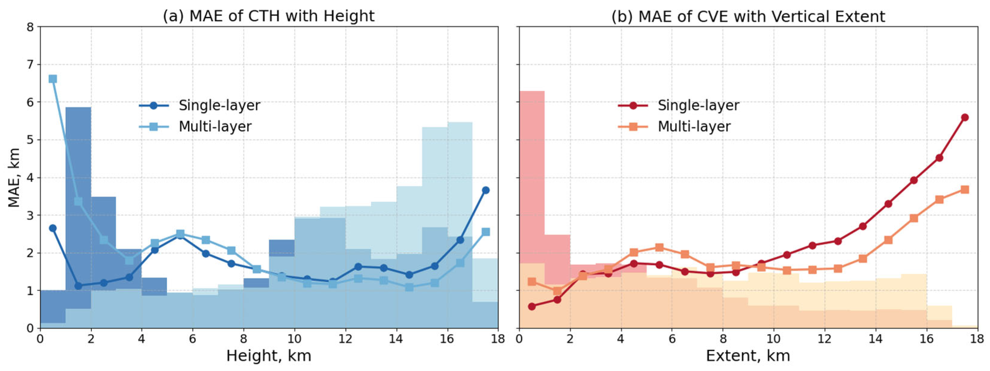
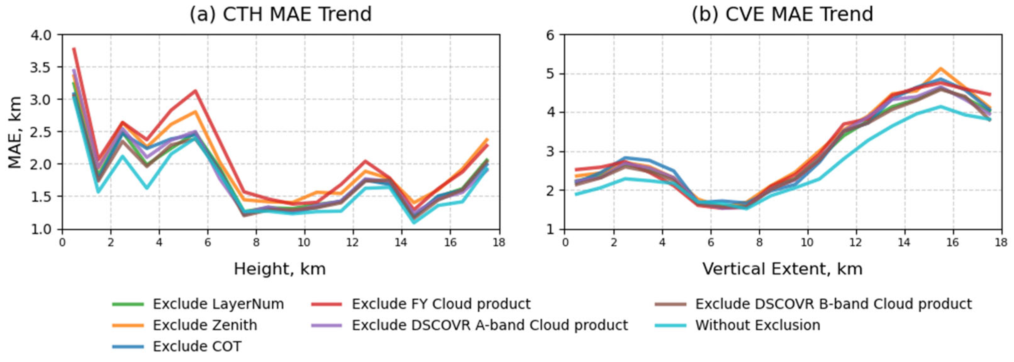
5.1. Error Source Analysis

Section 4.1 points out that the CLN model misclassifies some single-layer clouds as multi-layer clouds and vice versa. Therefore, it is necessary to assess how these misclassifications impact the performance of the CTH/CVE model. For clarity, we define Cloud 1 as all single-layer cloud samples (where n C = 1), Cloud 21 as double-layer clouds misclassified as single-layer clouds (where n C = 2, but n M = 1), Cloud 2 as all double-layer cloud samples (where n C = 2), and Cloud 12 as single-layer clouds misclassified as double-layer clouds (where n C = 1, but n M = 2).
Figure 8a–f compare the distribution probabilities of the above four cloud categories on CTH and CTT, and the data used are from the FY-4A and DSCOVR products. Cloud 1 (blue histogram) and Cloud 21 (blue line) exhibit similar distributions for both CTH and CTT, as do Cloud 2 (red histogram) and Cloud 12 (red line). However, Figure 8g,h demonstrate Cloud 1 and Cloud 21 have different vertical structures based on the true CTH and CVE from the CloudSat/CALIPSO products. This suggests that cloud misclassification stems from their cloud top properties appearing more similar to those of clouds with different layer numbers in passive remote sensing observations. For example, cases where thin cirrus overlies cumulus may be misclassified as single-layer clouds in passive remote sensing. The training process of the CLN model is susceptible to interference from clouds with different layer numbers but similar cloud top characteristics, resulting in cloud layer misclassification.
The samples with erroneous layer number labels may subsequently compromise the accuracy of both the CTH and CVE models. To validate this hypothesis, we designed a comparative experiment of using the true cloud layer number ( n C ) instead of the estimated values (obtained via the CLN model, n M ) as the input and retrained the CTH and CVE models. Figure 9 is the validation on the test set, and all the data used are the same as those in Figure 6.
Figure 9 shows the improvements in the CTH and CVE optimizations compared to Figure 6. Regarding the CTH, the R2 for single- and multi-layer clouds increases by 11% (from 0.69 to 0.80) and 10% (from 0.60 to 0.70), respectively. Meanwhile, the RMSE decreases from 3.0 km to 2.4 km for single-layer clouds and 2.7 km to 2.3 km for multi-layer clouds (achieving relative improvements of 20% and 14%). The MAE also reduces by 0.4 km for single-layer clouds and 0.2 km for multi-layer clouds.
The CVE optimization shows a better improvement than the CTH. R2 for single- and multi-layer clouds increases by 36% (from 0.43 to 0.79) and 32% (from 0.43 to 0.75), respectively. The RMSE shows remarkable optimization from 3.3 km to 2.0 km for single-layer clouds and from 3.6 km to 2.4 km for multi-layer clouds (achieving relative improvements of 40% and 33%). The MAE decreases by about 1.0 km for single- and multi-layer clouds.
Based on the above analysis, we infer that the reason for cloud layer misclassification stems from the similar appearance in passive remote sensing, and accurate cloud layer numbers can greatly improve the performance of the CTH and CVE optimization models.

5.2. Importance of Input Variables

We conducted an ablation experiment to evaluate the importance of input variables in the CTH and CVE optimizations. As shown in Figure 10, the input variables are divided into six groups: FY-4A cloud products (i.e., CTH ( h F ), CTT ( t F ), CTP ( p F ), CLT ( κ F ), CLP ( φ F )), DSCOVR A- and B-band cloud products (i.e., CTH ( h A   a n d   h B ), CTT ( t A   a n d   t B ), CTP ( p A   a n d   p B )), cloud optical thickness from DSCOVR (i.e., liquid and ice ( τ L and τ I )), geometric observation angles from DSCOVR (i.e., sensor and solar zenith angle ( ϑ D and θ D )), and number of layers ( n M ). The experiment excludes each group to obtain corresponding MAE–height trends. Additionally, the importance is quantified using LightGBM’s information gain metric [35], which measures the total information gain from feature splits, robustly capturing contributions in high-dimensional, non-linear systems.
The ablation experiments reveal significant MAE differences between the control group (without exclusion) and experimental groups, especially for low clouds (CTH < 5 km), thin clouds (CVE < 4 km), and thick clouds (CVE > 8 km), validating our feature selection.
Figure 10a shows the MAE for CTH optimizations. For instance, groups excluding FY-4A parameters or observation angles exhibit 1–2 km higher MAEs at 2–6 km altitudes, and excluding the cloud layer number also increases the MAE in this range, highlighting their importance. Furthermore, Figure 11a confirms that the FY-4A CTH is the most important input variable, followed by the cloud layer number.
Figure 10b shows the MAE for CVE optimizations. For clouds with a 4–8 km vertical extent, the MAE is consistent between experimental and control groups. Nevertheless, in other ranges, experimental groups’ MAEs differ by approximately 0.8 km from the control group. All experimental groups display similar trends across vertical extent ranges. Figure 11b identifies cloud layer number as being paramount for CVE optimizations, with FY-4A’s CTH/CTP and observation angles as being secondary important input variables.
Notably, Figure 11a,b reveal a different variable importance between CTH and CVE optimization. CTH depends more on cloud top parameters (height/pressure), while CVE relies on vertical structure information (e.g., layer number). The reliance on the cloud layer number corresponds to the discussion in Section 5.1 that using the true cloud layer number ( n C ) reduces the MAE by 16% for CTH and 38% for CVE, and it has the potential to improve the CTH/CVE optimization. In addition, FY-4A’s CTH/CTT ranks second in contributing to the CVE optimization.
It is worth noting that, although LightGBM’s gain metric highlights the cloud layer number as an important feature for both CTH and CVE models (Figure 11), its removal alone causes an MAE change comparable in magnitude to the removal of other entire feature groups (Figure 10). This seeming inconsistency may stem from the following:
1.
Other ablation groups removed multiple variables, whose combined effects amplified performance drops, making them comparable to the cloud layer number removal case;
2.
The cloud layer number provides classification information only and lacks direct height or vertical extent information, requiring interaction with other variables for a full effect.
The cloud layer number acts as a crucial prior constraint. It identifies multi-layer structures and separates error sources. Multi-layer clouds often indicate phase layering or greater vertical extent, thus adding the cloud layer number constrains the combinations of cloud top parameters and reduces ambiguity. As a structural classifier, the cloud layer number complements cloud top parameters, together enabling a more complete representation of cloud 3D structures.

5.3. Underlying Principles of the ML-Based Method

The models developed in this study estimate cloud vertical structure using only passive remote sensing observations from FY-4A and DSCOVR. This approach presents a fundamental challenge, as passive sensors inherently lack the ability to probe into clouds and directly measure their vertical profiles. Clarifying the feasibility of this approach is therefore essential. The following discussion elaborates on the underlying physical principles that enable this retrieval by leveraging the synergy between the two different sensor systems.
For CTH and CVE estimation, a key consideration is that passive retrievals yield ‘effective’ rather than true geometric values, as their signals are contaminated by radiation from within and below the cloud. Since FY-4A (TIR-based) and DSCOVR (O2-band-based) operate on different physics, the systematic patterns of this ‘contamination’ differ for each sensor when viewing the same cloud system. For instance, for a high, semi-transparent cirrus over a lower, warmer water cloud, the FY-4A TIR sensor will be biased low due to contamination from the warm emission below. The DSCOVR O2-band retrieval will also be biased as the lower cloud alters the effective photon path length, but this bias pattern is physically distinct from that of the TIR method. Our model learns to decode the discrepancy between these two different, biased measurements. By simultaneously analyzing both sets of products, the model can better constrain the true vertical location (CTH) and extent (CVE) of the cloud system, a task that is ill-posed for a single passive instrument.
For CLN estimation, the mechanism is likely more complex. We hypothesize that the model learns to distinguish between single- and multi-layer clouds by recognizing the different signatures they leave on the full suite of input variables. It is plausible that the complex inter-layer radiative interactions unique to multi-layer systems (e.g., multiple reflections, thermal trapping) create subtle, systematic patterns in the relationships between the various cloud top parameters. The CLN model may then learn to identify these multi-variate ‘fingerprints’ to perform its classification.

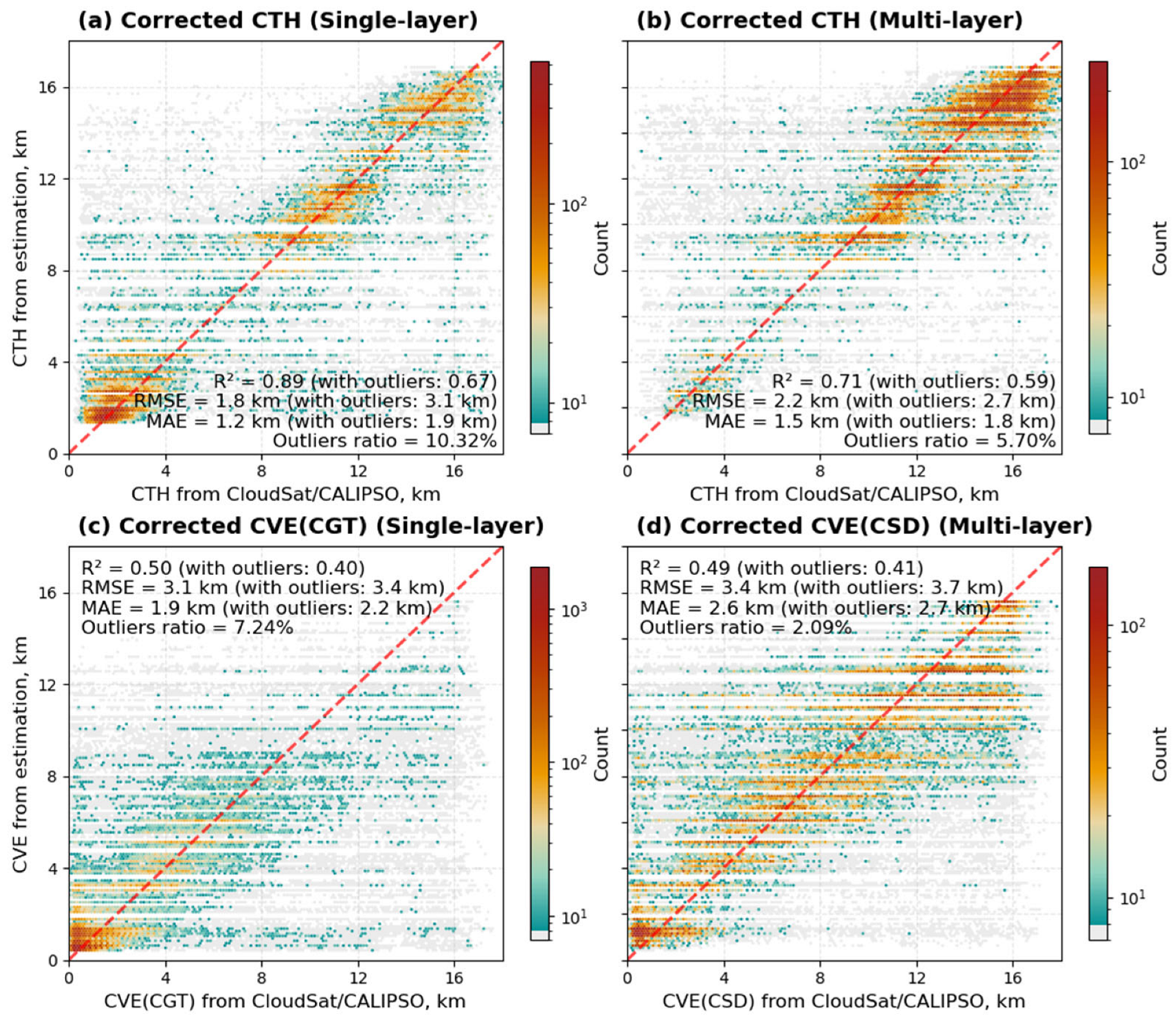
5.4. Post-Processing Bias Correction

A potential limitation of our results is the presence of systematic, magnitude-dependent biases, where CTH is overestimated for low clouds and underestimated for high clouds, with CVE exhibiting a similar pattern for thin and thick clouds, respectively. Given the clear pattern of systematic bias in our initial results, we investigated two distinct post-processing correction approaches to mitigate it: a piecewise linear regression, and a more complex data-driven calibration using a second LightGBM model.
While both methods were effective at reducing systematic bias, neither led to a significant improvement in overall accuracy metrics (R2, RMSE, MAE), which perhaps suggests that a more sophisticated correction technique is required than those we investigated. A detailed description of these experiments, including the methodology and comparative figures, is provided in Appendix B. We acknowledge, however, that exploring more advanced bias-correction techniques remains a valuable direction for future research.

6. Conclusions

This study presents a LightGBM-based algorithm for the optimization of cloud top height (CTH) and cloud vertical extent (CVE) by integrating the FY-4A and DSCOVR passive sensing cloud products. The algorithm enables high-frequency (hourly), high-accuracy, wide-area cloud vertical structure measurements. Validation based on CloudSat/CALIPSO shows MAEs of 2.0 km for the single-layer CTH, 2.3 km for single-layer cloud geometrical thickness (CGT), 2.7 km for multi-layer cloud system depth (CSD), and 1.8 km for multi-layer CTH, improving accuracy by 4–8 km over the FY-4A and DSCOVR products. The key findings are as follows:
The complementarity between cloud layer number and cloud top parameters (CTH/CTT/CTP) reveals a novel synergistic paradigm. The cloud layer number acts as a “structural classifier” providing vertical structure prior constraints through discrete labels (e.g., single- and multi-layer clouds), while cloud top parameters serve as “physical quantifiers” conveying radiative characteristics. Their combination effectively decouples systematic errors between FY-4A and DSCOVR.
The model demonstrates good performance in typical cloud systems: it achieves relatively small errors for the CTH/CVE of high-top thick clouds, but still faces challenges in characterizing vertically complex clouds due to the radiative signal aliasing effect, particularly in distinguishing single-layer clouds from multi-layer systems with similar cloud top properties. The experiment of using the true cloud layer number achieves the best accuracy and highlights the importance of reliable cloud layer classification for CTH and CVE estimations.
The optimization algorithm offers a new approach for the real-time monitoring of cloud vertical structure evolution. This method utilizes existing satellites to enhance the ability to observe the Earth, which is conducive to global-scale cloud water cycle monitoring and to improving the ability to track cloud vertical structural changes during extreme weather events. Moreover, the fundamental framework of this algorithm is not sensor-specific and could be readily adapted for use with other geostationary satellites, such as the GOES or Meteosat series, to potentially achieve near-global, high-frequency CVS monitoring.

Author Contributions

Conceptualization, Z.Z. and J.Y.; Data curation, Z.Z., T.L., and J.D.; Formal analysis, Z.Z., J.Y., Z.L., and S.L.; Investigation, Z.Z. and Y.Y.; Methodology, Z.Z. and Z.L.; Project administration, Z.L.; Software, Z.Z.; Validation, Z.Z.; Visualization, Z.Z.; Writing—original draft, Z.Z. and J.Y.; Writing—review and editing, Z.Z. and J.Y. All authors have read and agreed to the published version of the manuscript.

Funding

This research was funded by the National Natural Science Foundation of China (No. 42205129) and supported by the Open Fund of Hubei Luojia Laboratory (No. 250100011 and No. 250100008) and the Youth Project from the Hubei Research Center for Basic Disciplines of Earth Sciences (No. HRCES-202408).

Data Availability Statement

The raw data supporting the conclusions of this article will be made available by the authors on request.

Conflicts of Interest

The authors declare no conflict of interest.

Appendix A. Justification for Excluding Mixed-Phase Top-Layer Samples

The decision to exclude cloud profiles with a mixed-phase top layer from our final training dataset is based on a two-fold justification: a direct empirical assessment of our model’s performance and supporting evidence from recent large-scale validation studies.
First, we conducted a sensitivity analysis to empirically quantify the impact of including these samples. A parallel version of our model was trained and validated on a dataset that included profiles with a mixed-phase top layer, with the results presented here in Figure A1 and Figure A2. A direct comparison of these results with our final model’s performance (presented in Figure 5 and Figure 6 of the main text) reveals a clear and systematic degradation across all metrics. Taking the multi-layer cloud vertical extent (CVE) as a specific example, when the mixed-phase samples are included (Figure A2d), the Root Mean Squared Error (RMSE) increases to 3.9 km and the Mean Absolute Error (MAE) rises to 3.1 km. These values are substantially worse than those achieved by our final model, which excluded these samples (RMSE = 3.6 km, MAE = 2.8 km, as shown in Figure 6d). This confirms that including these samples has a tangible, negative impact on the model’s predictive accuracy.
Figure A1. Validation of the (a) CTH and (b) CVE model trained on the dataset that includes samples with a mixed-phase top layer. The light gray areas indicate bins with fewer than ten samples, while the remaining regions are color-coded based on data density. Outliers are identified using the IQR method. These results are presented for sensitivity analysis and should be compared with the model performance shown in Figure 5. The red dashed line is the 1:1 reference line, while the black solid lines represent segmented linear regression fits to the data excluding outliers.
Remotesensing 17 02484 g0a1
Figure A2. Validation of the optimized (a,b) CTH and (c,d) CVE models for the sensitivity test including samples with a mixed-phase top layer, separated by single- and multi-layer cloud conditions. The validation is performed for the following: (a) CTH for single-layer clouds, (b) CTH for multi-layer clouds, (c) cloud geometrical thickness (CGT) for single-layer clouds, and (d) cloud system depth (CSD) for multi-layer clouds. These results should be compared with the model performance shown in Figure 6. The red dashed line is the 1:1 reference line, while the black solid lines represent segmented linear regression fits to the data excluding outliers.
Remotesensing 17 02484 g0a2
Second, the recent literature provides a strong physical explanation for this observed performance degradation. We attribute this negative impact not to a failure of our model, but to the introduction of unreliable labels from the ground-truth dataset itself. A comprehensive validation study reveals that the 2B-CLDCLASS-LIDAR product exhibits a significant systematic bias: a notable overestimation of the mixed-phase cloud frequency, which likely stems from the misclassification of what are actually pure ice or pure liquid layers [24]. This finding corroborates our experimental results, suggesting that the “mixed-phase” labels are themselves often incorrect, thus introducing conflicting information and noise into our model’s training process.
In conclusion, given both the empirical evidence from our own sensitivity tests and the supporting findings from external validation studies, we determined that excluding profiles with a mixed-phase top layer was the most scientifically sound approach. This decision enhances the quality and reliability of our training dataset, ensuring our final algorithm is built upon the most accurate physical relationships possible.

Appendix B. Post-Processing Bias-Correction Experiment

Given the clear pattern of systematic bias in our results in Section 4.2, two distinct post-processing methods were implemented and evaluated to correct the systematic, magnitude-dependent biases observed in our initial cloud top height (CTH) and cloud vertical extent (CVE) estimation.

Appendix B.1. Piecewise Linear Regression Correction

The first approach utilized a piecewise linear regression. For both CTH and CVE, the dataset containing the initial model estimations and the corresponding ground-truth values was segmented into two parts using a threshold of 8 km in estimation. A separate linear regression model was then fitted to each segment. This method allowed the correction to adapt to the different bias characteristics observed for low versus high clouds and thin versus thick clouds. Figure A3 and Figure A4 show the validation results of the CTH and CVE models after applying the piecewise linear regression correction.
Figure A3. Validation of the (a) CTH and (b) CVE models after applying the piecewise linear regression correction. The light gray areas indicate bins with fewer than ten samples, while the remaining regions are color-coded based on data density. The red dashed line is the 1:1 reference line.
Remotesensing 17 02484 g0a3
Figure A4. Validation of the (a,b) CTH and (c,d) CVE models, similar to Figure A3. The difference is that the validation is carried out, respectively, on (a,c) single-layer clouds and (b,d) multi-layer clouds. The red dashed line is the 1:1 reference line.
Remotesensing 17 02484 g0a4
Table A1 and Table A2 compare the performance of two post-processing methods with that of the initial model for CTH and CVE estimation.
Table A1. Comparison of CTH estimation performance using different post-processing methods.
CTHInitial ModelLinear Regression CorrectionLightGBM Correction
R2RMSE (km)MAE (km)R2RMSE (km)MAE (km)R2RMSE (km)MAE (km)
Overall0.702.81.90.692.91.80.692.91.8
Single-layer0.693.02.00.673.11.90.673.11.9
Multi-layer0.602.71.80.592.71.80.592.71.8
Table A2. Comparison of CVE estimation performance using different post-processing methods.
CVEInitial ModelLinear Regression CorrectionLightGBM Correction
R2RMSE (km)MAE (km)R2RMSE (km)MAE (km)R2RMSE (km)MAE (km)
Overall0.503.52.60.483.52.40.483.52.4
Single-layer0.433.32.30.403.42.20.403.42.2
Multi-layer0.433.62.80.413.72.70.413.72.7

Appendix B.2. Data-Driven LightGBM Correction

The second approach involved training a data-driven calibrator. A second, lightweight LightGBM model was trained separately for CTH and CVE. This “correction model” learns the non-linear mapping from the initial model’s biased predictions (used as the single input feature) to the corresponding CloudSat/CALIPSO ground-truth values (used as the target). This method is designed to capture and remove more complex, non-linear systematic biases. Figure A5 and Figure A6 show the validation results of the CTH and CVE models after applying the data-driven LightGBM correction.
Figure A5. Validation of the (a) CTH and (b) CVE models after applying the data-driven LightGBM correction. The light gray areas indicate bins with fewer than ten samples, while the remaining regions are color-coded based on data density. The red dashed line is the 1:1 reference line.
Remotesensing 17 02484 g0a5
Figure A6. Validation of the (a,b) CTH and (c,d) CVE models, similar to Figure A5. The difference is that the validation is carried out, respectively, on (a,c) single-layer clouds and (b,d) multi-layer clouds.
Remotesensing 17 02484 g0a6

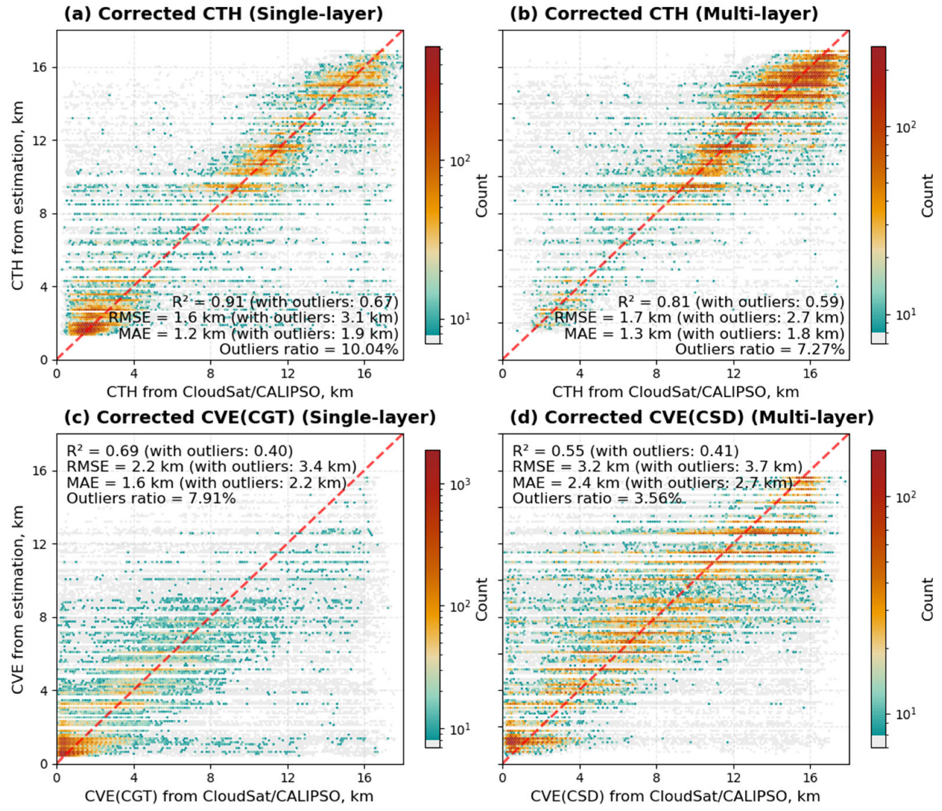
Appendix B.3. Analysis of the Correction Measurements

The effects of the two post-processing correction methods—piecewise linear regression and a data-driven LightGBM model—are summarized in Figure A3, Figure A4, Figure A5 and Figure A6. These can be compared against the original, uncorrected results presented in the main text (Figure 5 and Figure 6).
A visual inspection of the validation plots reveals that both correction methods were partially successful in their primary objective. For both the piecewise linear correction (Figure A3 and Figure A4) and the LightGBM correction (Figure A5 and Figure A6), the density of the data points is now visibly more centered around the 1:1 reference line. This indicates that both approaches were effective at mitigating the systematic, magnitude-dependent biases (i.e., the overestimation for low/thin clouds and the underestimation for high/thick clouds).
However, this reduction in systematic bias did not translate to an overall improvement in the models’ estimated accuracy. The statistical metrics (R2, RMSE, and MAE) across all four corrected figures show no significant improvement when compared to the uncorrected results. For instance, the R2 for CTH validation after piecewise correction is 0.69 with outliers (Figure A3a), which is identical to the 0.70 in Figure 5a. Furthermore, the R2 value for several cases decreased after the correction (e.g., from 0.48 to 0.41 for multi-layer CVE/CSD), suggesting a more significant dispersion.
While the post-processing methods investigated in this study did mitigate systematic biases, we have not yet identified a correction technique that robustly improves the model’s overall estimated accuracy. Therefore, the primary results presented in the main body of this study are those from the primary model without this additional post-processing step. We acknowledge, however, that exploring other, more sophisticated bias-correction techniques remains a valuable direction for future research.

References

  1. L’Ecuyer, T.S.; Hang, Y.; Matus, A.V.; Wang, Z. Reassessing the Effect of Cloud Type on Earth’s Energy Balance in the Age of Active Spaceborne Observations. Part I: Top of Atmosphere and Surface. J. Clim. 2019, 32, 6197–6217. [Google Scholar] [CrossRef]
  2. Stephens, G.L.; Vane, D.G.; Boain, R.J.; Mace, G.G.; Sassen, K.; Wang, Z.; Illingworth, A.J.; O’connor, E.J.; Rossow, W.B.; Durden, S.L.; et al. THE CLOUDSAT MISSION AND THE A-TRAIN: A New Dimension of Space-Based Observations of Clouds and Precipitation. Bull. Amer. Meteor. Soc. 2002, 83, 1771–1790. [Google Scholar] [CrossRef]
  3. Biondi, R.; Ho, S.; Randel, W.; Syndergaard, S.; Neubert, T. Tropical Cyclone Cloud-top Height and Vertical Temperature Structure Detection Using GPS Radio Occultation Measurements. JGR Atmos. 2013, 118, 5247–5259. [Google Scholar] [CrossRef]
  4. Lismalini; Marzuki; Shafii, M.A.; Yusnaini, H. Relationship between Cloud Vertical Structures Inferred from Radiosonde Humidity Profiles and Precipitation over Indonesia. J. Phys. Conf. Ser. 2021, 1876, 012011. [Google Scholar] [CrossRef]
  5. Hamada, A.; Nishi, N. Development of a Cloud-Top Height Estimation Method by Geostationary Satellite Split-Window Measurements Trained with CloudSat Data. J. Appl. Meteorol. Climatol. 2010, 49, 2035–2049. [Google Scholar] [CrossRef]
  6. Xu, W.; Lyu, D. Evaluation of Cloud Mask and Cloud Top Height from Fengyun-4A with MODIS Cloud Retrievals over the Tibetan Plateau. Remote Sens. 2021, 13, 1418. [Google Scholar] [CrossRef]
  7. Yang, Y.; Marshak, A.; Mao, J.; Lyapustin, A.; Herman, J. A Method of Retrieving Cloud Top Height and Cloud Geometrical Thickness with Oxygen A and B Bands for the Deep Space Climate Observatory (DSCOVR) Mission: Radiative Transfer Simulations. J. Quant. Spectrosc. Radiat. Transf. 2013, 122, 141–149. [Google Scholar] [CrossRef]
  8. Håkansson, N.; Adok, C.; Thoss, A.; Scheirer, R.; Hörnquist, S. Neural Network Cloud Top Pressure and Height for MODIS. Atmos. Meas. Tech. 2018, 11, 3177–3196. [Google Scholar] [CrossRef]
  9. Min, M.; Li, J.; Wang, F.; Liu, Z.; Menzel, W.P. Retrieval of Cloud Top Properties from Advanced Geostationary Satellite Imager Measurements Based on Machine Learning Algorithms. Remote Sens. Environ. 2020, 239, 111616. [Google Scholar] [CrossRef]
  10. Tan, Z.; Liu, C.; Ma, S.; Wang, X.; Shang, J.; Wang, J.; Ai, W.; Yan, W. Detecting Multilayer Clouds from the Geostationary Advanced Himawari Imager Using Machine Learning Techniques. IEEE Trans. Geosci. Remote Sens. 2022, 60, 4103112. [Google Scholar] [CrossRef]
  11. Tao, M.; Chen, J.; Xu, X.; Man, W.; Xu, L.; Wang, L.; Wang, Y.; Wang, J.; Fan, M.; Shahzad, M.I.; et al. A Robust and Flexible Satellite Aerosol Retrieval Algorithm for Multi-Angle Polarimetric Measurements with Physics-Informed Deep Learning Method. Remote Sens. Environ. 2023, 297, 113763. [Google Scholar] [CrossRef]
  12. Viggiano, M.; Cimini, D.; De Natale, M.P.; Di Paola, F.; Gallucci, D.; Larosa, S.; Marro, D.; Nilo, S.T.; Romano, F. Combining Passive Infrared and Microwave Satellite Observations to Investigate Cloud Microphysical Properties: A Review. Remote Sens. 2025, 17, 337. [Google Scholar] [CrossRef]
  13. Tan, Z.; Ma, S.; Zhao, X.; Yan, W.; Lu, W. Evaluation of Cloud Top Height Retrievals from China’s Next-Generation Geostationary Meteorological Satellite FY-4A. J. Meteorol. Res. 2019, 33, 553–562. [Google Scholar] [CrossRef]
  14. Heidinger, A.K.; Pavolonis, M.J.; Holz, R.E.; Baum, B.A.; Berthier, S. Using CALIPSO to Explore the Sensitivity to Cirrus Height in the Infrared Observations from NPOESS/VIIRS and GOES-R/ABI. J. Geophys. Res. 2010, 115, 2009JD012152. [Google Scholar] [CrossRef]
  15. Marshak, A.; Herman, J.; Adam, S.; Karin, B.; Carn, S.; Cede, A.; Geogdzhayev, I.; Huang, D.; Huang, L.-K.; Knyazikhin, Y.; et al. Earth Observations from DSCOVR EPIC Instrument. Bull. Am. Meteorol. Soc. 2018, 99, 1829–1850. [Google Scholar] [CrossRef] [PubMed]
  16. Ahn, C.; Torres, O.; Jethva, H.; Tiruchirapalli, R.; Huang, L. Evaluation of Aerosol Properties Observed by DSCOVR/EPIC Instrument From the Earth-Sun Lagrange 1 Orbit. JGR Atmos. 2021, 126, e2020JD033651. [Google Scholar] [CrossRef]
  17. Davis, A.B.; Merlin, G.; Cornet, C.; Labonnote, L.C.; Riédi, J.; Ferlay, N.; Dubuisson, P.; Min, Q.; Yang, Y.; Marshak, A. Cloud Information Content in EPIC/DSCOVR’s Oxygen A- and B-Band Channels: An Optimal Estimation Approach. J. Quant. Spectrosc. Radiat. Transf. 2018, 216, 6–16. [Google Scholar] [CrossRef]
  18. Davis, A.B.; Ferlay, N.; Libois, Q.; Marshak, A.; Yang, Y.; Min, Q. Cloud Information Content in EPIC/DSCOVR’s Oxygen A- and B-Band Channels: A Physics-Based Approach. J. Quant. Spectrosc. Radiat. Transf. 2018, 220, 84–96. [Google Scholar] [CrossRef]
  19. Kuze, A.; Chance, K.V. Analysis of Cloud Top Height and Cloud Coverage from Satellites Using the O2 A and B Bands. J. Geophys. Res. 1994, 99, 14481–14491. [Google Scholar] [CrossRef]
  20. Daniel, J.S.; Solomon, S.; Miller, H.L.; Langford, A.O.; Portmann, R.W.; Eubank, C.S. Retrieving Cloud Information from Passive Measurements of Solar Radiation Absorbed by Molecular Oxygen and O2-O2. J. Geophys. Res. 2003, 108, 2002JD002994. [Google Scholar] [CrossRef]
  21. Weisz, E.; Li, J.; Menzel, W.P.; Heidinger, A.K.; Kahn, B.H.; Liu, C. Comparison of AIRS, MODIS, CloudSat and CALIPSO Cloud Top Height Retrievals. Geophys. Res. Lett. 2007, 34, 2007GL030676. [Google Scholar] [CrossRef]
  22. Wang, W.; Sheng, L.; Dong, X.; Qu, W.; Sun, J.; Jin, H.; Logan, T. Dust Aerosol Impact on the Retrieval of Cloud Top Height from Satellite Observations of CALIPSO, CloudSat and MODIS. J. Quant. Spectrosc. Radiat. Transf. 2017, 188, 132–141. [Google Scholar] [CrossRef]
  23. Sassen, K.; Wang, Z. Classifying Clouds around the Globe with the CloudSat Radar: 1-year of Results. Geophys. Res. Lett. 2008, 35, 2007GL032591. [Google Scholar] [CrossRef]
  24. Wang, D.; Yang, C.A.; Diao, M. Validation of Satellite-Based Cloud Phase Distributions Using Global-Scale In Situ Airborne Observations. Earth Space Sci. 2024, 11, e2023EA003355. [Google Scholar] [CrossRef]
  25. Watts, P.D.; Bennartz, R.; Fell, F. Retrieval of Two-Layer Cloud Properties from Multispectral Observations Using Optimal Estimation. J. Geophys. Res. 2011, 116, D16203. [Google Scholar] [CrossRef]
  26. Yang, Y.; Meyer, K.; Wind, G.; Zhou, Y.; Marshak, A.; Platnick, S.; Min, Q.; Davis, A.B.; Joiner, J.; Vasilkov, A.; et al. Cloud Products from the Earth Polychromatic Imaging Camera (EPIC): Algorithms and Initial Evaluation. Atmos. Meas. Tech. 2019, 12, 2019–2031. [Google Scholar] [CrossRef] [PubMed]
  27. Upadhyay, A. Haversine Formula-Calculate Geographic Distance on Earth. 2015. Available online: Https://Www.Igismap.Com/Haversine-Formula-Calculate-Geographic-Distance-Earth/ (accessed on 18 May 2025).
  28. Bley, S.; Deneke, H.; Senf, F. Meteosat-Based Characterization of the Spatiotemporal Evolution of Warm Convective Cloud Fields over Central Europe. J. Appl. Meteorol. Climatol. 2016, 55, 2181–2195. [Google Scholar] [CrossRef]
  29. Grosvenor, D.P.; Wood, R. The Effect of Solar Zenith Angle on MODIS Cloud Optical and Microphysical Retrievals within Marine Liquid Water Clouds. Atmos. Chem. Phys. 2014, 14, 7291–7321. [Google Scholar] [CrossRef]
  30. Ke, G.; Meng, Q.; Finley, T.; Wang, T.; Chen, W.; Ma, W.; Ye, Q.; Liu, T.-Y. LightGBM: A Highly Efficient Gradient Boosting Decision Tree. In Proceedings of the 31st Conference on Neural Information Processing Systems (NIPS 2017), Long Beach, NY, USA, 4–9 December 2017. [Google Scholar]
  31. Xuan, L.; Lin, Z.; Liang, J.; Huang, X.; Li, Z.; Zhang, X.; Zou, X.; Shi, J. Prediction of Resilience and Cohesion of Deep-Fried Tofu by Ultrasonic Detection and LightGBM Regression. Food Control 2023, 154, 110009. [Google Scholar] [CrossRef]
  32. Alshboul, O.; Almasabha, G.; Shehadeh, A.; Al-Shboul, K. A Comparative Study of LightGBM, XGBoost, and GEP Models in Shear Strength Management of SFRC-SBWS. Structures 2024, 61, 106009. [Google Scholar] [CrossRef]
  33. Breiman, L. Random Forests. Mach. Learn. 2001, 45, 5–32. [Google Scholar] [CrossRef]
  34. Hodge, V.; Austin, J. A Survey of Outlier Detection Methodologies. Artif. Intell. Rev. 2004, 22, 85–126. [Google Scholar] [CrossRef]
  35. Hajihosseinlou, M.; Maghsoudi, A.; Ghezelbash, R. A Novel Scheme for Mapping of MVT-Type Pb–Zn Prospectivity: LightGBM, a Highly Efficient Gradient Boosting Decision Tree Machine Learning Algorithm. Nat. Resour. Res. 2023, 32, 2417–2438. [Google Scholar] [CrossRef]
Figure 1. A comparison of the cloud top heights of FY-4A/DSCOVR along with CloudSat/CALIPSO, respectively, in the single-layer cloud systems in the first row and the multi-layer cloud systems in the second row. The y-axis values in the first column are from FY-4A, the second column are from DSCOVR’s oxygen A-band, and the third column are from DSCOVR’s oxygen B-band. The red dashed line is the 1:1 reference line.
Remotesensing 17 02484 g001
Figure 2. The mean error (ME) variations in the FY-4A and DSCOVR cloud top height products. The solid and dashed lines represent multi-layer and single-layer cloud systems, respectively. The lines represent the DSCOVR A-band (blue), DSCOVR B-band (red), and FY-4A (yellow) products, respectively.
Remotesensing 17 02484 g002
Figure 3. An example showing temporal variations in FY-4A imagery (yellow), DSCOVR imagery (blue), and CloudSat/CALIPSO orbital tracks (red).
Remotesensing 17 02484 g003
Figure 4. The confusion matrices of CLN models trained using the cloud layer number (a) before and (b) after adjustment. Clouds with more than seven layers are excluded.
Remotesensing 17 02484 g004
Figure 5. Validation of the (a) CTH and (b) CVE model. Ten-fold cross-validation is used. The light gray areas indicate bins with fewer than ten samples, while the remaining regions are color-coded based on data density: warm colors (orange) signify high-density areas, and cool colors (cyan) signify low-density areas. Outliers are identified using the IQR method. The red dashed line is the 1:1 reference line, while the black solid lines represent segmented linear regression fits to the data excluding outliers.
Remotesensing 17 02484 g005
Figure 6. Validation of the optimized (a,b) CTH and (c,d) CVE models, separated by single- and multi-layer cloud conditions. The validation is performed for the following: (a) CTH for single-layer clouds, (b) CTH for multi-layer clouds, (c) cloud geometrical thickness (CGT) for single-layer clouds, and (d) cloud system depth (CSD) for multi-layer clouds. The red dashed line is the 1:1 reference line, while the black solid lines represent segmented linear regression fits to the data excluding outliers.
Remotesensing 17 02484 g006
Figure 7. Mean Absolute Error (MAE) of the optimized model estimations as a function of the true cloud properties from CloudSat/CALIPSO. (a) Estimated CTH MAE binned by reference CTH. (b) Estimated CVE MAE binned by reference CVE. The dark lines and corresponding dark histograms represent single-layer cloud systems, while the light lines and light histograms represent multi-layer systems. Background histograms show their respective sample distributions, with the y-axis in each panel scaled uniformly to allow for a direct comparison of sample counts between single- and multi-layer clouds.
Remotesensing 17 02484 g007
Figure 8. Frequency distributions of various cloud properties for four distinct cloud categories. The (ac) CTH and (df) CTT frequency distributions of four cloud categories are based on the data from DSCOVR and FY-4A products. The (g) CTH and (h) CVE frequency distributions are based on the data from the CloudSat/CALIPSO products. The blue histogram is for single-layer clouds (Cloud 1). The red histogram is for double-layer clouds (Cloud 2). The blue line is for double-layer clouds wrongly classified as single-layer clouds (Cloud 21). The red line is for single-layer clouds wrongly classified as double-layer clouds (Cloud 12). PDF refers to the Probability Density Function.
Remotesensing 17 02484 g008
Figure 9. Validation of the optimized (a,b) CTH and (c,d) CVE models that were trained using the true cloud layer number ( n C ) as the input, and the other parameters and methods used are the same as in Figure 6, including that (a,c) single- and (b,d) multi-layer clouds are still categorized based on the estimated cloud layer number ( n M ). The red dashed line is the 1:1 reference line, while the black solid lines represent segmented linear regression fits to the data excluding outliers.
Remotesensing 17 02484 g009
Figure 10. The MAE of optimized CTH/CVE across height and vertical extent (1 km bins). Colored lines indicate experiments excluding specific inputs, i.e., number of layers (LayerNum, n M ), solar/sensor angles (zenith), cloud optical thickness (liquid/ice COT), FY-4A products (CTH/CTT/CTP/CLT/CLP), or DSCOVR A/B-band products (CTH/CTT/CTP). The baseline (without exclusion) retains all input variables.
Remotesensing 17 02484 g010
Figure 11. Importance of each input variable based on information gain. (a) The importance of each input for the CTH model. (b) The importance of each input for the CVE model. DSA and DSB represent the cloud top properties retrieved from the DSCOVR A- and B-bands.
Remotesensing 17 02484 g011
Table 1. Inputs for training the CLN, CTH, and CVE estimation models.
ModelInputLabel
CLN   ( n M )      FY - 4 A :   h F ,   t F ,   p F
DSCOVR :   h A ,   t A ,   p A ,   h B ,   t B ,   p B ,   τ L ,   τ I ,   ϑ D ,   θ D
CloudSat / CALIPSO :   n C
CTH/CVE      FY - 4 A :   h F ,   t F ,   p F ,   φ F ,   κ F
DSCOVR :   h A ,   t A ,   p A ,   h B ,   t B ,   p B ,   φ D ,   τ L ,   τ I ,   ϑ D ,   θ D
    CLN :   n M
CloudSat / CALIPSO :   h C ,   l C
Table 2. Hyperparameter configurations for the CLN, CTH, and CVE estimation models.
HyperparameterCLN ModelCTH/CVE ModelDescription
boosting_typegbdtgbdtGradient Boosting Decision Tree
n_estimators10,00010,000Number of boosting iterations
learning_rate0.0050.005Step size shrinkage
max_depth1010Maximum tree depth
num_leaves380300Maximum number of leaves per tree
bagging_fraction0.750.75Fraction of data to be used for each iteration
feature_fraction0.750.75Fraction of features to be used for each iteration
objectivemulticlassregressionSpecifies the learning task and objective
Table 3. The evaluation metrics of the original and optimized cloud top height.
All CloudsSingle-Layer CloudsMulti-Layer Clouds
R2RMSE (km)MAE (km)R2RMSE (km)MAE (km)R2RMSE (km)MAE (km)
FY-4A−0.095.54.00.453.92.6−2.856.65.4
DSCOVR A-band−1.157.76.5−0.065.54.2−6.759.48.9
DSCOVR B-band−1.528.37.1−0.306.14.7−7.9010.19.5
New Model0.702.81.90.693.02.00.602.71.8
Disclaimer/Publisher’s Note: The statements, opinions and data contained in all publications are solely those of the individual author(s) and contributor(s) and not of MDPI and/or the editor(s). MDPI and/or the editor(s) disclaim responsibility for any injury to people or property resulting from any ideas, methods, instructions or products referred to in the content.

