Early Detection of Soil Salinization by Means of Spaceborne Hyperspectral Imagery

Abstract

Soil salinization is increasingly affecting agricultural areas worldwide, reducing soil quality and crop yields. Surface salinization evidences present complex spectral features, increasing in depth with increasing salt concentrations. For this reason, low salinization detection provides a complex challenge to test the capabilities of new-generation hyperspectral satellites. The aim of this study is to test the capability of the new generation of hyperspectral satellites (EnMAP) in detecting early stages and low levels of topsoil salinization and to investigate the differences between laboratory and image spectra to take into account their influence on model performance. The area of study, the Grosseto plain, located in central Italy, presented heterogeneous salinity levels ($E{C}_{max}$= 11.7 dS/m, $E{C}_{mean}$= 0.99 dS/m). We investigated the salt-affected soil spectral behaviour with both laboratory-acquired spectra ($n_{obs}$= 60) and EnMAP-derived spectra ($n_{obs}$= 20). Both datasets were pre-processed with multiple data transformation algorithms and 2D correlograms, PLSR and the Random Forest regressor were tested to identify the best model for salinity detection. Two-dimensional correlograms resulted in an $R^2$ of 0.88 for laboratory data and 0.63 for EnMAP data. PLSR proved to have the worst performance. The Random Forest regressor proved its capability in detecting complex spectral features, with $R^2$ scores of 0.72 for laboratory data and 0.60 for EnMAP. The Random Forest model provides very satisfactory mapping capabilities when tested on the whole study area. The results highlight that the EnMAP-derived dataset produces similar results to those of ASD laboratory spectra, providing evidences regarding EnMAP’s predictive capability to detect early stages of topsoil salinization.

1. Introduction

Climate change is altering seasonal weather patterns and dynamics, impacting terrestrial systems and soil properties. This results in less rain, higher temperatures, and more extreme precipitation events [1,2]. The modification of climate patterns will deteriorate soil properties by increasing erosion, cause a decline in organic matter and lead to salinisation [3], in a time where global food production is needed to increase by a predicted maximum of 62% by 2050 [4]. To ensure global food security, no further soil depletion phenomena can be left untackled. Globally, soil salinization is responsible for soil loss accounting for 1069 Mha in 2016, with an increase of 16.8% for the period 1986–2016 [5]. It is therefore important to develop a large-scale and reliable methodology to monitor and assess the impacts of salinity on soils. New-generation hyperspectral satellites such as EnMAP and PRISMA open up new possibilities for soil salinization detection and monitoring. Their spectral resolution will enable the study and detection of early phenomena traits previously undetectable at the satellite scale. For this reason, the present paper will adopt a demonstrative approach to test new-generation hyperspectral satellites’ capabilities for detecting early soil salinization, projecting the insights derived from laboratory spectroscopy to the spaceborne platform.

Saline soils are defined by the Soil Science Society of America as a non-sodic soil containing sufficient amount of soluble salt which could adversely influence crop plants [6]. Soil salinity is measured by soil electrical conductivity ($E{C}_e$) computed on a soil–water paste extract or dilution (1:5) and classified according to the work of Richards [7];

Table 1. Classification of soil salinity classes produced by Richards [7], defined for soil electrical conductivity and its corresponding effect on crop plants.

Soil Salinity Class	Electrical Conductivity (dS/m)	Effect on Crop Plants
Non saline	0–2	Negligible salinity effects
Slightly saline	2–4	Yields of sensitive crops may be restricted
Moderately saline	4–8	Yields of many crops are restricted
Strongly saline	8–16	Only tolerant crops yield satisfactorily
Very strongly saline	≥16	Only a few very tolerant crops yield satisfactorily

.

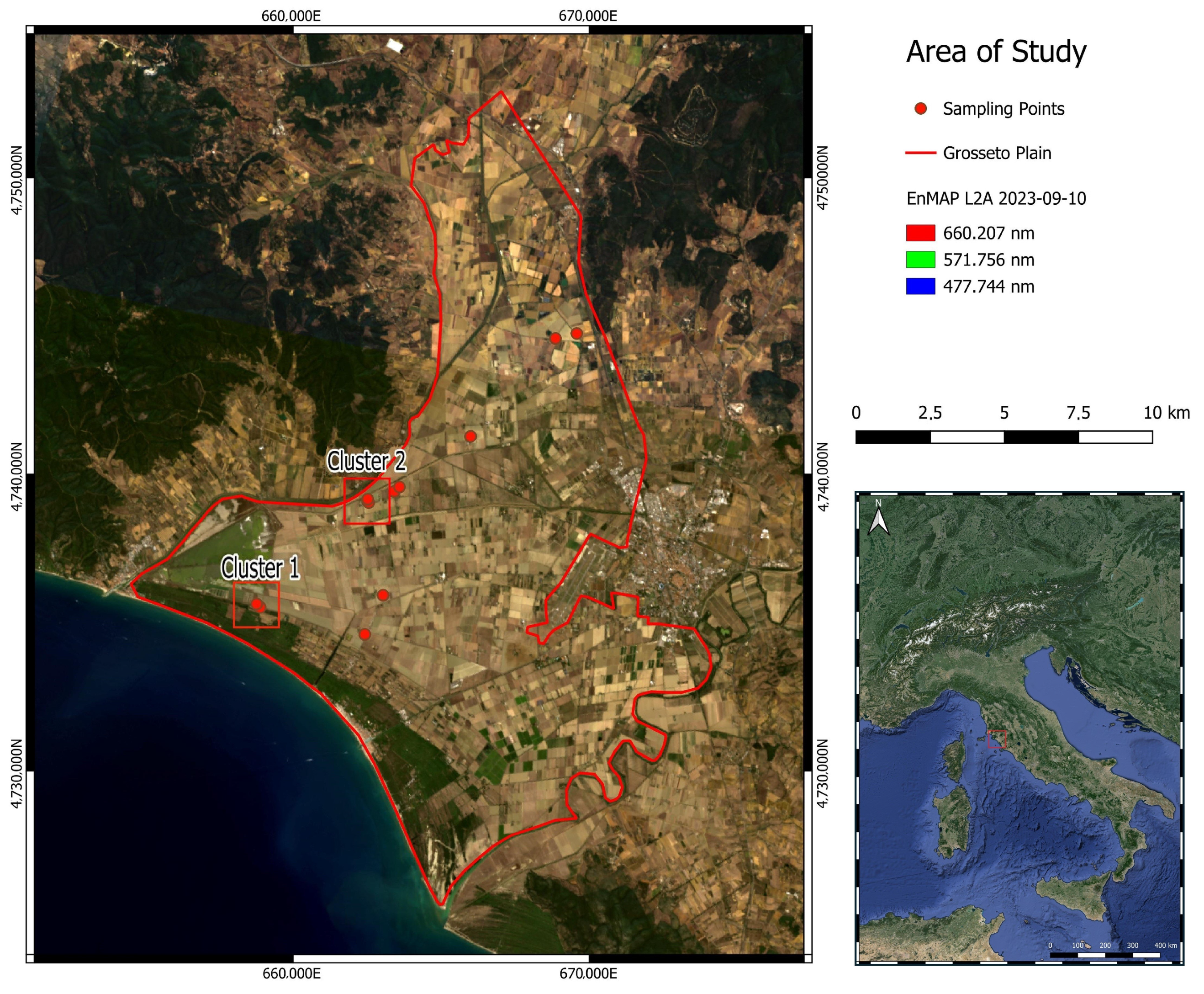
According to Rengasamy [8], irrigation-associated salinity occurs when salts introduced by irrigation water are stored in the root zone because of insufficient leaching. This type of salinization is commonly observed in areas with poor irrigation water quality, low hydraulic conductivity and a strong deficit of evapotranspiration on precipitation, this being the case of the area of interest. In addition, land management practices such as irrigation, crop type and fertilization practices strongly influence the occurrence of salinization [8]. In coastal areas, the expected sea level rise and intrusion provides favourable conditions for an increase in soil salinization [9]. In addition, the over-exploitation of groundwater might result in saltwater wedge intrusion, contaminating the freshwater reservoir and increasing the water cation–anion concentration. When such contaminated water is used for irrigation, plant evapotranspiration removes water (solvent) while the cations and anions (solute) precipitate in the soil column, crystallizing as salts. Therefore, repeated applications of brackish water increase the soil salt concentration. In addition, the decreased precipitation regime resulting from climate change is not sufficient to leach the salts out of the soil horizons. Surface evidences of this phenomenon strongly depend on pedology, soil texture and surface condition, together with climate and topography [2]. Depending on the magnitude of soil salinization and the above-mentioned parameters, topsoil evidences manifest with salt efflorescence or crusts [10].

Optical remote sensing has proven to be a useful tool in the assessment of many environmental-related phenomena [11,12]. More specifically, satellite platforms allow for a site scale and cost-effective analysis, enabling decision-makers to develop management strategies based on the condition of the asset. With salinization globally increasing and threatening such a fundamental resource as soil, many authors have tested optical remote sensing imagery from multi-spectral sensors [13,14,15] and hyper-spectral sensors [16,17,18,19] for their capability in detecting salt evidences on vegetation or soil. Refs. [16,19,20,21,22] proved the efficacy of hyperspectral remote sensing for salt detection in many salt types and contexts. Different approaches have been proposed to map salinization focussing on soil. These methods include multispectral indices, narrow-band hyperspectral indices, machine learning and linear regression, such as PLSR. Notably, method performances are influenced by salinization magnitude, where moderate to high salinization areas are easily detected while low salinity levels and initial stages of salinization frequently cause identification failures [10,23,24]. For this reason, in this paper we will assess the capabilities of new hyperspectral satellite imagery of the EnMAP mission in detecting initial stages of salinization.

Hyperspectral remote sensing has been applied for soil salinization assessment based on airborne campaigns or first hyperspectral space-borne demonstrators such as HYPERION on board EO-1 [25]. In recent years, new hyperspectral space-borne missions with high data quality were launched, such as PRISMA in 2019 [26] and EnMAP in 2022 [27]. Their specifications should enable greater capacity to characterize the extent and severity of variable stages of salinization. The high spectral resolution of the new sensors allows one to resolve with more precision and accuracy the elements contributing to the spectral signature, therefore opening new possibilities for the analysis of diagnostic features not previously exploitable [28]. In addition, improvements in the radiometric resolution results in a greater range of representable values of radiance measured by the sensor. Moreover, the onboard calibration instruments allow for homogeneous and constant spectral measurements across different scenes, providing a solid base for spectral signatures comparability. All things considered, geometric and spectral resolution require precise geolocation of the measured pixel [29].

Ground observations and radiometric measurements indicate how salt-affected soil reflectance is primarily influenced by the quantity and mineralogy of salts, as well as soil moisture, colour and roughness [19,25]. Among these parameters, moisture significantly influences the spectral behaviour of salt-affected soils, shifting the regions of high and low reflectance in the spectra [10]. The mineralogy of salts, such as carbonates, sulfates and chlorides, depending on the crystallization pattern, dictates the presence or absence of absorption features in the electromagnetic spectrum. More light is trapped in coarse lattices (e.g., gypsum) than in fine lattices (e.g., halite), resulting, for example, in no diagnostic absorption features in the Visible and Near-Infrared (VNIR) and Short-Wave Infrared (SWIR) spectral regions for pure halite [30]. Additionally, the absorption features observed in the VNIR-SWIR range for salt efflorescence spectra primarily arise from the internal vibration modes of anion groups or water molecules trapped, adsorbed or associated with the crystal structure [31].

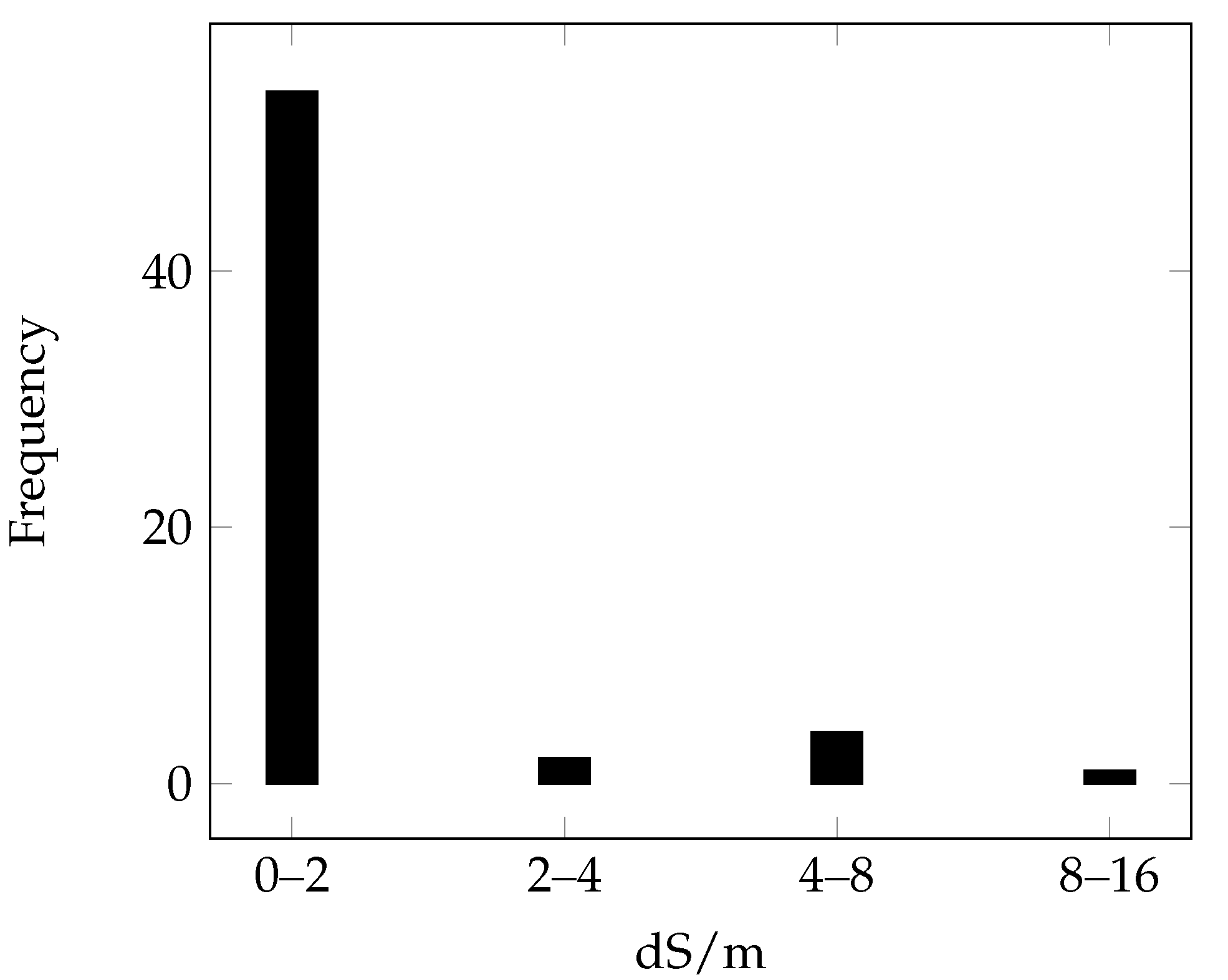
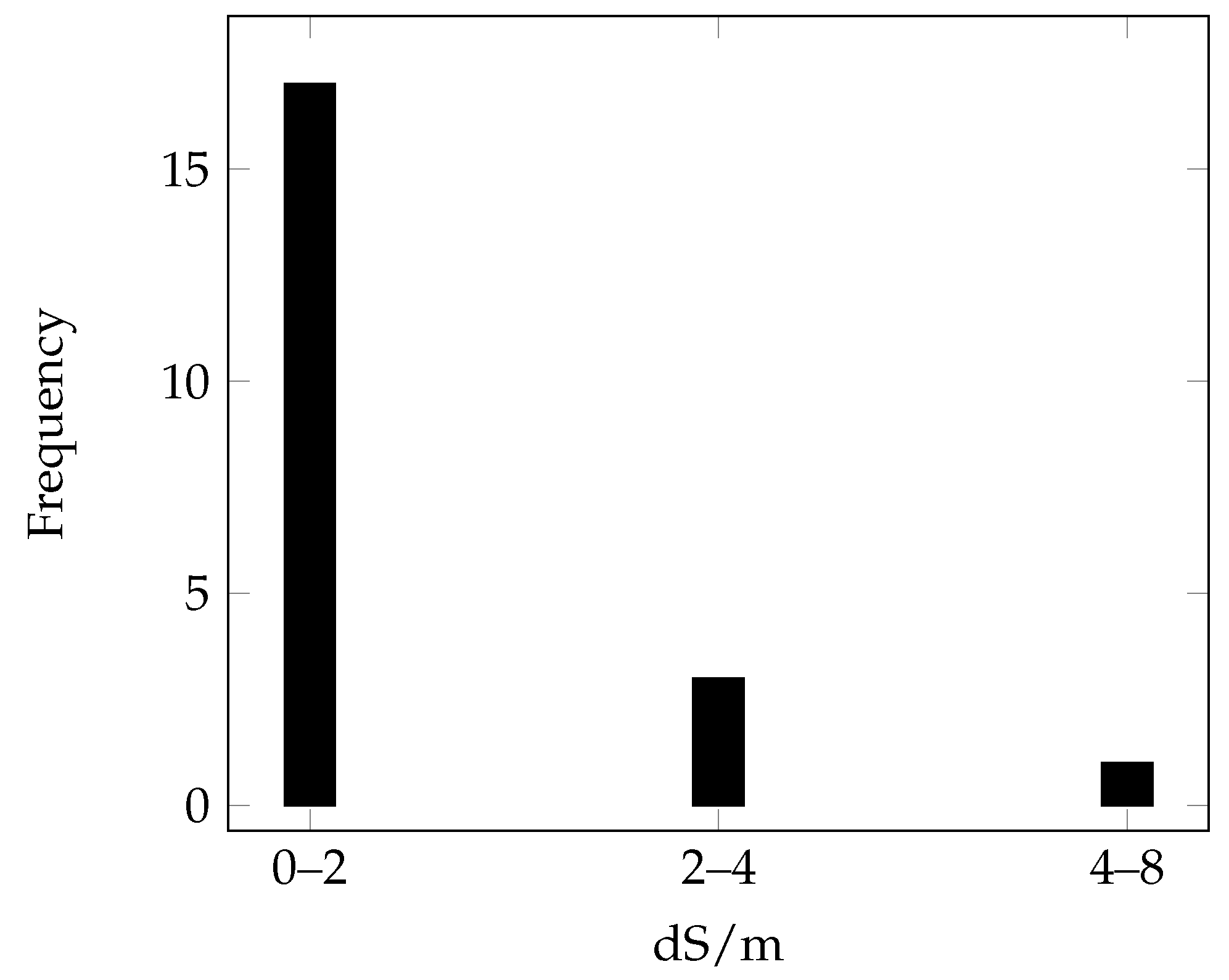
The literature review of remote sensing techniques for soil salinization manifests a developed suite of methodologies in use for salinization mapping. Nevertheless, the approaches examined are tested and implemented mostly on case studies with high levels of salinization, therefore leaving a gap in the early detection of the phenomena, when remediation actions could be more effective. For this reason, this paper aims to test the capability of the new generation of hyperspectral satellites such as EnMAP in detecting early stages and low levels of topsoil salinization. Early stages of salinization were defined as soils with $EC\le 2$ dS/m, according to the classification produced by Richards [7]; Table 1. Concomitantly, we investigated the differences occurring between laboratory and image spectra to take into account their influence on model performance.

2. Materials and Methods

2.1. Study Site

The Grosseto plain, 42°46.00^′N 10°57.19^′E, is located in the southern part of Tuscany, Italy. The climatic type is maritime Mediterranean with an average temperature of 15.7 °C and 600 mm precipitations [32]. The geomorphology of the area is prevalently flat with small altitude variations in the plain (under 5 m of variation), delimited by the terminal portion of the Bruna and Ombrone rivers, north and south, resulting in an extension of 350 ${\mathrm{km}}^2$, with 29,000 ha of agricultural fields. Its geographical setting is bounded by the Castiglione della Pescaia hills to the west, the Montepescali hills to the north-east, the hills of Grosseto and Ripescia to the south-east and by the Uccellina hills to the south. The alluvial plain is composed of Quaternary deposits, such as cemented sand dunes and loose coastline sand and conglomerates of fluvial terraces coupled with gravel and sand, all bounding the plain. More to the centre, recent travertine depositions and prevalently clay-rich alluvial deposits can be found [33].

The plain has undergone a long swamp reclamation process via the ‘colmata’ technique, an artificial aggradation by the deposition of river-borne sediments [34]. This was achieved with the creation of channels conveying water coming from the hills into the main water-courses and the positioning of four water pumps to accelerate the ‘colmata’ process and drainage water removal. This solution shaped the Grosseto plain into what it is nowadays, a highly impacted landscape and a large agro-touristic ecosystem [34].

Evidences of water and soil salinization were acknowledged starting from 1935, when shore-side water wells proved to be unsuitable for agricultural and human use because of high salt content. In the past century, salinization was limited to spot-specific areas but has since then increased to a greater extent. In times with low anthropogenic pressure, salinization was mainly caused by the intrusion of seawater via the hydrographical network during storms and was affecting clayey areas with poor drainage [34,35]. Concomitantly, nowadays water deficit during the irrigation season is higher than 400 mm, and more than 70% of the irrigation water is drawn from the groundwater table [34]. The combination of water deficit in the area with the onset of intensive agriculture disrupted the reservoir equilibrium, with seawater intruding into the freshwater reservoir used for irrigation [36]. Additionally, depending on well location, thermal water from Triassic evaporite reservoirs or gypsum leaching waters is extracted, resulting in high electrical conductivity waters despite the coastline–well distance [37].

Figure 1 presents the RGB EnMAP composite of the two concomitantly acquired tiles for the area of interest. Sampling points in cluster 1 proved to have the highest salt content according to EC laboratory analysis. Observing Figure 2, for cluster 1 it is possible to note how, in images a and b, surface efflorescence occurrence is a function of the distance from the drainage channel. In Figure 2c,d, on the other hand, it is possible to appreciate how the sub-metric depression at the top of the cultivated field presents an accumulation of salt, testified by its surface evidences. For cluster 1, both occurrences of surface manifestations are related to the topography and drainage network. On the other hand, Figure 2e,f, for cluster 2, present surface salt manifestations as a consequence of dripping irrigation applied to watermelon crops.

2.2. Field and Satellite Data

2.2.1. EnMAP Specifications

EnMAP (Environmental Monitoring and Analysis Program), the new German scientific hyperspectral mission, is characterized by unprecedented data quality and pixel positioning precision. Deployed on 1 April 2022, it began its routine operations on 2 November 2022. The satellite operates a pushbroom sensor, covering a spectral range from 420 to 2450 nm and offering global coverage. It captures data across 228 spectral bands, with sampling intervals of 6.5 nm in the VNIR channel and 10 nm in the SWIR channel. The geometric spatial resolution is 30 m, and the maximum swath width is 30 km, with a maximum acquisition length of 1200 km. The sensor radiometric resolution of ≥14 bit guarantees high spectral detail of the acquired spectra. The advancements testified by the new generation of hyperspectral satellites also come with a pixel geolocation error of 0.69 pixel offset for EnMAP, when compared to a Sentinel-2 reference image [38] and VNIR-SWIR co-registration accuracy of 0.1 pixels [29]. Overall, the mission characteristics represent an innovative instrument for Earth observation, enabling new applications and use-case scenarios.

Figure 1. EnMAP image of the study site in true colour representation [39,40]. Sampling points (red circles) result as clustered as a consequence of the scale of representation. The area delimited by the red square polygon represents the Grosseto plain.

Figure 1. EnMAP image of the study site in true colour representation [39,40]. Sampling points (red circles) result as clustered as a consequence of the scale of representation. The area delimited by the red square polygon represents the Grosseto plain.

Figure 2. Field images for clusters 1 and two spatially positioned according to Figure 1. Images (a–d) for cluster 1 present salinization as a consequence of topography—presence of local depressions linked to drainage channel. Images (e,f) for cluster 2 show the occurrence of salinization as a consequence of anthropic irrigation—drip irrigation pipe buried between the crop rows.

Figure 2. Field images for clusters 1 and two spatially positioned according to Figure 1. Images (a–d) for cluster 1 present salinization as a consequence of topography—presence of local depressions linked to drainage channel. Images (e,f) for cluster 2 show the occurrence of salinization as a consequence of anthropic irrigation—drip irrigation pipe buried between the crop rows.

2.2.2. Field Sampling Campaign and Laboratory Analysis

Field sampling was conducted at the apex of the dry season in late September 2023, to maximize the salinization surface evidences. To minimize the effects of the phenomenon high temporal and spatial variability the field campaign was planned to have the shortest time gap between satellite acquisition and field measurements. The phenomenon of high variability and the study’s demonstrative approach motivated the selection of a limited number of samples. The German hyperspectral satellite, EnMAP, acquired data over the area of interest on September the 10th [39,40]. The atmospheric conditions for the satellite acquisition and field campaign days were clear, with no clouds and excellent visibility. The field campaign took place on the 5th and the 12th. Samples collected on the two dates are distinct, contributing to the population of the whole dataset. In the time window defined by the first and last campaign day, no precipitation occurred, ensuring the invariance of surface efflorescence manifestation and magnitude. The field sampling strategy was structured to minimize the spectral contamination of non-target elements. Consequently, points were selected in areas with fewest mixed elements (e.g., by vegetation, buildings, roads, water), ensuring object homogeneity in a 60 × 60 m area surrounding the sampling point. The acquisition procedure for each site consisted of a cross-shaped geometry with segments of 15 m length. Starting from the centre of the cross, five samples were collected, one in the centre and four at the end of each line. This geometry was chosen to optimize the number of samples to process in the lab while taking into account the spatial variability of the phenomenon. The twelve field collection sites resulted in 60 samples collected on a clear sky day with no previous precipitations. To avoid any topsoil disturbance, the sample’s spectral signature was first collected; successively, the surface material was scraped and the point GPS position acquired. The spectral signature acquisitions were performed using the Malvern Pananlytical ASD Fieldspec 4 [41]. Field spectral signatures were acquired with the instrument’s bare fibre and with constant fiber-ground height. Prior to any acquisition, instrument optimization was performed and the white reference spectra saved.

The sixty soil samples were then processed according to FAO soil salinization assessment procedure to measure the soil electrical conductivity (ECe) [42]. ECe was calculated using the 1:5 water–soil dilution method, measured with an XS REVio multiparametric electrode [43]. Six samples with the highest salinity were also analyzed with X-ray diffractometry (XRD) to identify salt minerals. An Anton Paar XRDynamic 500 diffractometer (Co-K$\alpha$1, 40 kV × 50 mA) with a Pixos 2000 detector and monochromator was used. Data were collected over a 5–${\mathrm{70}}^{\circ }$ 2$\theta$ range (${\mathrm{0.03}}^{\circ }$ step, 100 s/step) using the X’Pert PRO Philips system, confirming the presence of halite as major salt species.

Together with the field spectral signatures, we collected laboratory soil spectra using the black box protocol by [44] for each sample. The acquisitions were performed following the laboratory methodology defined in [45]. Both the field and laboratory spectra were processed to remove the portable spectroradiometer detection unit jumps. For this paper, only laboratory-acquired spectra were used in the model training and analysis. For field spectra, the atmospheric absorption bands were removed, followed by smoothing operated with a Savitzky–Golay [46] filter (window size 11 nm and third-order polynomial).

2.2.3. Satellite Data Acquisition

EnMAP Bottom of Atmosphere (BOA) products (L2A) were downloaded from the EnMAP archive, EOWEB Geoportal, on 10 October 2023 EnMAP acquisition, being pre-processed to L2A and acquired over clear sky conditions, did not require any correction. Within the image, the spectra of the pixels were extracted corresponding to the soil sampling points. As the image pixel position in relation to the sampling site is a priori unknown, more than one field measure was bounded by a pixel. Within these pixels, the field-derived $E{C}_e$ values were averaged. As a consequence, from the 60 field samples collected, 21 EnMAP-derived spectra were associated with chemical lab data.

2.3. Salinization Modelling

Laboratory and EnMAP image spectra have been analysed with different approaches [47], assessing their capability in resolving such a spectrally and spatiotemporally complex phenomenon as salinization.

The analysis methodology followed a two-step process:

• Models test on laboratory-acquired soil spectral signatures
• Models test on EnMAP-derived spectral library

In the first step, laboratory spectral signatures were used to assess the different pre-processing and model performances. The analysis statistical significance was the first prerequisite to determine the feasibility of early salinization detection in soil samples. In the second step, EnMAP image spectra were pre-processed and the models tested for performance. According to the statistical metrics, the best model was selected and deployed on the whole image, evaluating its capability to predict salinity levels for unknown spectra. Prior to model deployment, the image was masked for Photosynthetic Vegetation (PV), Non-Photosynthetic Vegetation (NPV) and anthropic features.

Models Tested

The three approaches tested include 2D correlograms computation, Partial Least Squares Regression (PLSR) and the Random Forest (RF) regression model. All modelling approaches have been tested on Reflectance (R) and on pre-processing techniques to assess the optimal data condition for the specific approach. For the Savitzky–Golay dataset (SG) [46], to test the effect of spectral artefacts introduced by atmospheric correction algorithms, sections of the spectra related to water vapour were masked, and the gap interpolated, further applying a Savitzky–Golay filter with a window size of 11 nm and third order polynomial. In addition to the above-mentioned SG dataset, the pre-processing algorithms tested were Continuum Removal (CR) [48], Principal Component Analysis (PCA) [49], Norris Gap first (FD) and Second Derivatives (SD) [50]. The metrics used for model performance assessment were $R^2$ [51], RMSE [52] and RPD [49].

$$R^2=1-{\displaystyle \frac{{\sum }_{i=1}^n{(y_i-{\widehat{y}}_i)}^2}{{\sum }_{i=1}^n{(y_i-\overline{y})}^2}}$$

(1)

$$\mathrm{RMSE}=\sqrt{{\displaystyle \frac{1}{n}}\sum _{i=1}^n{(y_i-{\widehat{y}}_i)}^2}$$

(2)

$$\mathrm{RPD}={\displaystyle \frac{\mathrm{SD}}{\mathrm{RMSE}}}$$

(3)

where

$$\mathrm{SD}=\sqrt{{\displaystyle \frac{1}{n-1}}\sum _{i=1}^n{(y_i-\overline{y})}^2}$$

(4)

where $y_i$ is the measured value of EC, ${\widehat{y}}_i$ is the predicted value of EC, ${\overline{y}}_i$ is the mean of the observed values and n is the number of samples involved in regression analysis.

Two-dimensional correlograms for narrow band hyperspectral indices were computed according to [20], as the methodology achieves satisfactory results returning the best band couple related to the target variable [53]. Nawar suggests three mathematical index combinations to assess the best-performing wavelength pair for each index, evaluating its capability in estimating the target variable, $E{C}_e$, considering the maximum variance explained by the wavelength pair. The index structures for Difference Index (DI), Normalized Difference Index (NDI) and Ratio Index (RI) were:

$$\mathrm{DI}(R_i,,R_j)=R_i-R_j$$

(5)

$$\mathrm{NDI}(R_i,,R_j)={\displaystyle \frac{(R_i-R_j)}{(R_i+R_j)}}$$

(6)

$$\mathrm{RI}(R_i,,R_j)={\displaystyle \frac{R_i}{R_j}}$$

(7)

Among the tools used to map soil properties, PLS regression proved its value in managing data with severe collinearity in the independent variable, as the superimposing spectral absorptions of soil [20,54,55,56]. PLSR was selected from the various regression algorithms as it represents a benchmark for imaging spectroscopy-derived soil parameters. The model was optimized by searching for the optimal number of PLS components capable of minimizing the error metrics.

RF regressor was implemented with the Python (v3.10) Sklearn library, optimized for the analysis with hyperparameter tuning using the sklearn halving grid search tool [57]. The optimization allowed for the definition of the best model parameters to predict the target variable from the spectra in the dataset. The parameters tested for optimization are summarized in

Table 2. Random Forest hyperparameters tested in model optimization for laboratory and satellite spectra.

Parameters	Variables
Criterion	gini, entropy, log loss, Friedman-mse
Max features	sqrt, $lo{g}_2$, None
Minimum samples leaf	2, 4
Minimum samples split	2, 10
Maximum depth	10, 20, None
Number of estimators	400, 800, 1000

. The calibration–validation of the model was performed with Leave One Out Cross Validation (LOOCV) using the whole observations dataset.

3. Results

3.1. Effect of Salinity on Spectra

3.1.1. Laboratory Soil Spectra

Laboratory-acquired soil spectral signatures manifested two broad absorption features at 1400 and 1900 nm, in accordance with the information found in the literature [18,20,22]. In addition, it was possible to appreciate how different levels of salinity influenced the sample reflectance. Indeed, as shown in Figure 3, non-saline samples have the highest reflectance, progressively decreasing for moderately-saline and strongly-saline samples, with the latter manifesting the lowest reflectance. Absorption features around 1000, 1200, 1400 and 1900 nm in hydrated minerals are related to anion group vibrations. These features exhibit broad absorption due to overlapping water molecule bands in highly hydrated minerals, while less hydrated ones display narrower bands. Broad absorption bands near 1400 and 1900 nm in halite and thendarnite spectra are linked to fluid inclusions and/or absorbed water [31]. For all salt efflorescences, soil spectra show consistent absorption features at 1440 and 1933 nm, while for halite and sylvite it is possible to observe a trend of increasing absorption depths with increasing salt concentration [19]. This evidence is also supported by [20], reporting the presence of major halite-related absorption features at 415 and 1915 nm, with several weak absorption regions near 494, 673, 1748, 2276 and 2385 nm. Additionally, as hygroscopic salts can absorb water vapour, soil moisture increases with increasing salinization. It is also important to take into account how the soil surface roughness influences the spectral response. For example, the reflectance for cultivated non-saline surfaces decreases because of higher roughness produced by large clods in ploughed areas [10].

3.1.2. Satellite Soil Spectra

It is foremost important to acknowledge that the collected field samples do not cover an area comparable to EnMAP’s pixel geometric resolution. As a consequence, it is possible to experience a mismatch between the field-measured salinity and the satellite-sensed spectral response. To partially overcome this issue, pixels bounding more than one field measurement were assigned the average salinity level of the samples falling within the pixel boundary.

Differently from the ASD laboratory-acquired spectra, the EnMAP-derived soil spectra cannot rely on the wide absorption features centered at 1400 and 1900 nm, as they are affected by atmospheric water absorption. Additionally, the satellite-derived spectra seem to behave differently for the tested salinity levels. Figure 4 shows that the EnMAP spectrum with the highest salinity has the lowest reflectance only for the VIS region of the spectra, while for the NIR and SWIR region, the moderately saline sample has comparably lower reflectance. On the other hand, for laboratory spectra, higher salinization corresponds to lower reflectance. In addition, the satellite-derived spectra show the presence of mixed vegetation components in the pixel, concordant with field observations.

3.2. Salinity Modelling Based on Lab Data

3.2.1. Laboratory Data

The chemical data associated with the laboratory spectral signatures, calculated using the 1:5 water soil dilution method, are summarised in Figure 5.

3.2.2. Two-Dimensional Correlograms

The computation of the correlograms for ASD-acquired spectra resulted in the best index-band combinations, reported in

Table 3. Two-Dimensional correlograms computed for ASD- and EnMAP-derived spectral signatures.

ASD		EnMAP
Index-Band (nm)	${\mathit{R}}^{\mathbf{2}}$	Index-Band (nm)	${\mathit{R}}^{\mathbf{2}}$
DI ($R_{2017}$, $R_{2118}$)	0.27	DI ($R_{2068}$, $R_{2130}$)	0.61
NDI ($R_{370}$, $R_{2451}$)	0.45	NDI ($R_{2068}$, $R_{2130}$)	0.62
RI ($R_{382}$, $R_{2451}$)	0.52	RI ($R_{2068}$, $R_{2130}$)	0.63
DI ($S{G}_{2107}$, $S{G}_{2118}$)	0.27	DI ($S{G}_{510}$, $S{G}_{520}$)	0.53
NDI ($S{G}_{370}$, $S{G}_{2451}$)	0.45	NDI ($S{G}_{2014}$, $S{G}_{2407}$)	0.60
RI ($S{G}_{382}$, $S{G}_{2451}$)	0.52	RI ($S{G}_{2014}$, $S{G}_{2407}$)	0.62
DI ($C{R}_{396}$, $C{R}_{2004}$)	0.37	DI ($C{R}_{459}$, $C{R}_{473}$)	0.61
NDI ($C{R}_{449}$, $C{R}_{460}$)	0.38	NDI ($C{R}_{459}$, $C{R}_{473}$)	0.61
RI ($C{R}_{460}$, $C{R}_{449}$)	0.38	RI ($C{R}_{459}$, $C{R}_{473}$)	0.61
DI ($F{D}_{373}$, $F{D}_{1910}$)	0.63	DI ($F{D}_{482}$, $F{D}_{501}$)	0.62
RI ($F{D}_{1911}$, $F{D}_{657}$)	0.88	RI ($F{D}_{1484}$, $F{D}_{1518}$)	0.60

. Among the different indices, the Ratio Index (RI) provides the best coefficient of correlation, with an $R^2$ of 0.88 for the first derivative. The second-best performing index was the difference index, with an $R^2$ of 0.63 for the first derivative. However, except for the first derivative, the difference index did not perform well. From a pre-processing perspective, the first derivative presents the best scores, followed by reflectance and SG, with similar performance and continuum removal again settling on the lowest performance for all indices. Reflectance and SG filtered data share the same wavelength pairs for the considered indices, with the best combination resulting to be 382 and 2451 nm. The continuum-removed dataset generally resulted in the selection of wavelengths in the range of 400 nm, with an exception for the difference index, where, despite the poor $R^2$ score, the best pair resulted to be 396 and 2004 nm. First derivative selected wavelengths focus on the promising 1900 nm and red (650 nm) range; Figure 6. It should be noted how the chosen wavelengths, despite their high correlation with the target variable, should also be interpreted in light of other known absorption features within the selected ranges. Moreover, it is important to observe that, for the second derivative, the computation of the indices resulted to be unfeasible as a consequence of the numerical transformation of the spectra. Indeed, in the second derivative transformation, where the spectra does not present peaks or absorptions, its value is plotted as zero, impairing the mathematical computation. The same reason can account for the computation of the NDI for the first derivative.

3.2.3. PLSR

The best performing linear regression was obtained with the second Norris gap derivative, with $R^2$ of 0.51, RMSE of 1.29 and RPD 1.44; scores are summarized in

Table 4. PLS and Random Forest regression for ASD laboratory-acquired spectra.

	PLSR			Random Forest
	${\mathbf{R}}^{\mathbf{2}}$	RMSEM	RPD	${\mathbf{R}}^{\mathbf{2}}$	RMSE	RPD
R	0.29	1.55	1.20	0.42	1.41	1.31
CR	0.42	1.41	1.32	0.60	1.17	1.58
FD	0.17	1.68	1.11	0.37	1.46	1.26
SD	0.51	1.29	1.44	0.47	1.35	1.37
PCA	-	-	-	0.23	1.62	1.13
CR + PCA	-	-	-	0.72	0.98	1.89

. Differently from the results of the 2D correlograms, the second-best performing pre-processing for PLSR resulted to be the continuum-removed dataset $R^2$ 0.42, RMSE 1.41, RPD 1.32. Overall, the RPD scores for the PLS regression reveal the model’s capability in qualitatively assessing the parameter, but it lacks reliability for accurate quantitative predictions. Nevertheless, the RPD score for the second derivative shows how this pre-processing is useful for semi-quantitative predictions. The analysis also pointed out how both reflectance and first Norris derivative share the poorest statistical significance and great RMSE. Overall, PLSR regression proved to suffer from the high number of variables present in the ASD-acquired spectra.

3.2.4. Random Forest Regressor

Overall, RF model performance according to RMSE and RPD was satisfactory, with the results summarized in Table 4, especially considering the samples’ salinity distribution. Of all datasets, continuum-removed spectra show the best performance, with an increase obtained with the coupling of CR with twenty principal components (summarized in

Table A1. Five most relevant PCA principal components for the ASD CR + PCA dataset computed with permutation. Rows represent wavelengths (nm).

PC1	PC2	PC3	PC4	PC5
1908	1531	493	2237	1789
1907	1530	494	2238	1790
1909	1529	489	2236	1788
1906	1532	490	2239	1791
1910	1533	495	2235	1792
1905	1528	492	2240	1787
1904	1534	486	2234	1793
1903	1527	491	2241	1794
1911	1535	487	2233	1786
1902	1526	488	2242	1795
1912	1536	496	2232	1785
1901	1537	497	2243	1784
1900	1525	498	2231	1796
1913	1538	485	2244	1797
1899	1524	499	2230	1783
1898	1539	484	2245	1798
1897	1523	483	2229	1782
1914	1540	482	2228	1799
1896	1522	500	2164	1772
1895	1521	501	2165	1800
1915	1541	481	2163	1781
1894	1520	502	2162	1771
1916	1519	503	2167	1775
1893	1542	480	2166	1776
1917	1518	828	2168	1773
1892	1543	479	2161	1774
736	1517	478	2169	1777
735	1516	504	2227	1780
738	1544	505	2160	1770
739	1515	829	2246	1778
1918	1514	477	2170	1801
734	1545	832	2159	1779
737	1513	506	2226	1802
1891	1546	476	2171	1769
740	1512	475	2172	1866
733	1547	507	2158	1803
741	1511	508	2225	1865
732	1548	831	2173	1867
731	1510	474	2157	1768
730	1549	509	2224	1804

), with a 0.72 $R^2$ score achieved with the hyperparameters reported in

Table 5. Random Forest hyperparameters for CR + PCA pre-processing.

Parameters	Variables
Criterion	Friedman-mse
Max features	none
Minimum samples leaf	2
Minimum samples split	2
Maximum depth	10
Number of estimators	1000

. Notably, for this pre-processing, the 1.89 RPD score highlights the regressor performance, validating the model’s capability in estimating soil salinity. The second-best performing pre-processing was found to be the second Norris gap derivative, with an $R^2$ score of 0.47, coupled with a not-so-convincing RPD of 1.37. This performance can be linked to the transformation of the spectra operated by the second derivative, enhancing the reflectance variation with the spectral regions. Similarly to PLS regression, reflectance data suffer the high data collinearity deriving from ASD spectral sampling resolution, impairing the model performance in defining the best variables to predict salinity. The first Norris gap derivative, independently of the model applied for prediction, provides poor results also with Random Forest. In Figure 7, it is possible to see the results of the regression plots for ASD RF.

3.3. Satellite Data

The distribution of the 21 EnMAP-derived spectra associated with chemical data is summarized in Figure 8.

3.3.1. Two-Dimensional Correlograms

The 2D correlograms show a relevant statistical significance, with the highest $R^2$ value for the reflectance-based ratio index, taking advantage of the 2068–2130 nm band combination ($R^2$ 0.63); Table 3, Figure 6. It is interesting to observe how the $R^2$ scores of the satellite-derived datasets produces similar scores independently from the index definition. It is, however, clear that different pre-processing procedures affect the result of the correlograms. Despite the small $R^2$ variation, SWIR-based indices seem to perform better than the VIS-based ones. Additionally, the selection of SWIR wavelengths for the correlogram computation is less susceptible to colour variations of the topsoil, therefore increasing the robustness of the index. It is nevertheless interesting to observe how, despite lacking defined absorption features in the satellite spectra, the continuum-removed dataset performs in accordance with reflectance, Savitzky–Golay and the first derivative.

The best performing EnMAP index–wavelength according to Table 3 (Ratio Index) was then computed over the whole bare soil EnMAP image for the area of interest. To translate the index results to quantitative EC values, we calibrated the index results with the field-sampled conductivity parameters, performing a linear regression and computing the corresponding offset and gain values. The result of this operation allowed us to compare the salinity levels across different methods, such as the RF predictions based on the common unit of measurement of conductivity; Figure 9. The so obtained map shows poor regressive capabilities for the salinity in the area while pointing out the index bias towards unmasked anthropic elements.

3.3.2. PLSR

The application of PLSR on EnMAP-derived spectra did not provide satisfactory results. As can be observed by

Table 6. PLS and Random Forest regressions for EnMAP-derived spectral signatures.

	PLSR			Random Forest
	${\mathit{R}}^{\mathbf{2}}$	RMSE	RPD	${\mathit{R}}^{\mathbf{2}}$	RMSE	RPD
R	−0.12	2.55	0.58	0.59	0.62	1.56
SG	−3.89	3.19	0.46	0.60	0.61	1.57
CR	−1.78	2.13	0.69	0.1	0.95	1.00
FD	−1.59	2.32	0.63	0.45	0.72	1.34
SD	−0.99	2.04	0.72	0.44	0.72	1.34
PCA	-	-	-	0.1	0.93	1.03
CR + PCA	-	-	-	−0.12	1.02	0.94

, the $R^2$ shows a negative correlation for all pre-processing techniques, with a maximum negative value of −3.89 for SG. In support of this result comes the RMSE, higher than any other analysis performed. Consequently to the performance highlighted by the above-mentioned statistical metrics, it comes with no surprise how the RPD actually has the lowest scores across the regression models tested, showing how the model’s predictive capability is no better than using the mean of the observations. The poor results obtained with PLSR could be linked to the EnMAP dataset size, counting only twenty-one entries.

3.3.3. Random Forest Regressor

Despite the sample size, satisfactory model results were obtained (Figure 7, Table 6). The performance of the different pre-processing datasets is similar for reflectance, Savitzky–Golay and first derivative. The RPD and RMSE scores for the above-mentioned datasets are generally very similar, with the best model performance associated with the SG dataset and the model hyperparameters shown in

Table 7. Random Forest hyperparameters for SG dataset.

Parameters	Variables
Criterion	Friedman-mse
Max features	none
Minimum samples leaf	2
Minimum samples split	2
Maximum depth	none
Number of estimators	400

. Differently from the model scores tested with the ASD spectra, the EnMAP first derivative seems to have a better predictive accuracy than what has been previously seen. On the other hand, the continuum-removed dataset seems to decrease the model performance, possibly as a result of the absence of diagnostic absorption features linked to salinization. Overall, considering the satellite-based spectra, the application of Random Forest to the available datasets produces satisfactory results. The SG RF model was then applied to the whole EnMAP scene to estimate areas suffering from low salinization levels; Figure 10.

4. Discussion

The objective of this study was to evaluate the effectiveness of the new generation of hyperspectral satellites, such as EnMAP, in detecting early stages and low levels of topsoil salinization. Additionally, we examined the differences between laboratory and image spectra to assess their impact on model performance.

4.1. Laboratory Models

4.1.1. ASD 2D Correlograms

Our results show that the selected wavelengths mainly focus on the band pairs 1911–657 nm, 373–1910 nm and 382–2451 nm. The available literature supports the selected spectral ranges for salinity detection. Indeed, Sidike et al. [58] report that salinity sensitive bands fall in the ranges 350–436 nm, 516–814 nm, 1445–1506 nm, 1667–1699 nm, 1882–2096 nm and 2160–2393 nm. In addition, for laboratory acquisitions, Wang et al. [59] identified bands in the 1970–2450 nm range to be diagnostic for NaCl, the prevalent salt mineral species in the area of study.

The correlograms $R^2$ and the literature evidences support the findings regarding the correlogram capability in identifying salinity diagnostic bands. Wang et al. [53] propose using spectral subsets to increase the correlograms efficiency. However, for small salt concentrations and the possible presence of multiple salt mineralogy, our study shows that using the whole spectra for the 2D correlogram computation benefits the detection capabilities of the technique. Additionally, the computation of the best index–wavelength pairs on the full spectrum allows for better comparability across multiple datasets and sensing platforms (e.g.,: different pre-processing techniques), as the strongest diagnostic features might be in different spectral ranges on different sensing platforms. Correlograms, indeed, can be used as an exploratory methodology for the individuation of defining features associated with the target, before the development and deployment of more complex models [20]. The results obtained with ASD laboratory-acquired spectra are strongly influenced by the index mathematical structure and dataset pre-processing techniques. It is interesting to observe how the transformation of the data with the first derivative obtains the best output, independently of the index. Indeed, the literature highlights the presence of the 1400 and 1900 nm absorption features that, with the first derivative transformation, produce a significant signal that the correlogram leverages. The performance of FD pre-processing can be addressed to the transformation the derivative operates on the spectra, enhancing relative differences between spectral bands and reducing the baseline drift. Interestingly, the best index combination, RI ($F{D}_{1911}$, $F{D}_{657}$), couples the 1900 nm absorption feature with 657 nm, a wavelength in the red region of the spectra highlighting how soil colour might be influenced by salinization [53]. The performance of DI, RI and NDI is identical for both reflectance and Savitzky–Golay filtered data. This evidence does not belittle the correlogram performance but stresses the need to test an SG filter with a different window size compared to the one used. It comes as no surprise that spectra acquired in a controlled environment suh as a laboratory do not suffer from noise that could be removed with an SG filter. Surprisingly, despite the presence of distinct absorption features, the best index–wavelength pairs do not leverage a combination of both spectral ranges within the absorption feature ranges (1440 and 1900 nm).

4.1.2. PLS Regression

PLS regression for lab signatures did not obtain significant scores, despite the literature supporting the model robustness [60]. The $R^2$ scores prove how the model has a mediocre capability in predicting sample salinity from the spectral signatures. In addition, RPD scores support the information extrapolated by $R^2$, for which the model’s capability in predicting the target variable is scarce, as well as for the second derivative. Among the different pre-processings tested, the score obtained by the second derivative highlights how PLSR leverages the spectral variation for the considered bands but still lacks the capacity to consider greater spectral ranges. This deficiency impairs the model’s capability of extrapolating patterns in complex phenomena, where the overall spectra reflectance could play a role in the regression of the target variable.

4.1.3. Random Forest Regressor

Referring to the research question, the results obtained with the RF regressor can be considered very satisfactory, proving the model’s capability in predicting low levels of salinization from spectral signatures. The RPD score for the CR + PCA pre-processing proves the training of a robust model. Observing the statistical parameters for the transformations tested (Table 4), differently from PLSR, the decisional structure of RF takes advantage of the absorption characteristics and reduction of dimensions operated with an optimized number of components for PCA. Further investigating the PCA spectral ranges reveals the importance of wavelengths in the range 650 to 740 nm and 1890 to 1920 nm; Figure 11. Similarly, the RF regressor permutation for the CR and SD datasets showcases accordance with the relevance of the aforementioned ranges. These evidences support the assumption that salts, especially halite, produce secondary absorption features as a consequence of the salt hygroscopic effect, therefore manifesting in the water absorption region [61]. Moreover, the CR and SD permutation results highlight the relevance of additional wavelengths falling within the ranges 1150 to 1200 nm and 1920 to 2080 nm; Figure 11.

4.2. Satellite Models

4.2.1. Two-Dimensional Correlograms

Our study shows that the best diagnostic band couples rely on the wavelengths 1484–1518 nm, 2068–2130 nm and 2014–2407 nm. Not having a direct literature validation for new-generation hyperspectral satellite salinity diagnostic bands, we may infer that the spectral ranges individuated by Sidike et al. [58] from surface soil reflectance can be used as validation for satellite-derived spectra. In addition, Weng et al. [62] points out that reflectance in the ranges 1931–2123 nm and 2153–2254 nm is highly correlated with soil salt content. Furthermore, Srivastava et al. [63], using visible-near infrared reflectance spectroscopy, points out how the spectral range 1390–2400 nm is highly sensitive to salinization. The results of the correlogram computation firstly highlight the quality of EnMAP-derived spectra, as the R and SG filtered results are extremely close. Moreover, the bands selected for the DI computed on the SG filtered dataset, DI ($S{G}_{510}$, $S{G}_{520}$), $R^2$ 0.53, actually result in a worst performance compared to the corresponding index for the R dataset DI ($R_{2068}$, $R_{2130}$) $R^2$ 0.61. It is interesting to note that, despite the different signal transformations operated, the best index according to $R^2$ is derived for the R dataset, RI ($R_{2068}$, $R_{2130}$), $R^2$ 0.63, with the second-best performing index being RI ($S{G}_{2014}$, $S{G}_{2407}$), $R^2$ of 0.62. This statement is supported by the wavelengths selected for the R index computation, being reported by Wang et al. [53], whereas, despite the similar coefficient of determination, other index–wavelength combinations such as CR and FD rely on VIS or proximal band combinations only. As an example, observing the atmospheric transmittance windows reported by Thompson et al. [61], the wavelengths selected for RI-FD, 1484 and 1518 nm, as a consequence of their proximity with atmospheric absorption features, could easily be misleading regarding the concentration of the target variable.

Despite RI ($R_{2068}$, $R_{2130}$) being the best index–wavelength combination, sun-glint deriving from the sea surface saturated pixels for bands 2068–2130 nm, impairing the index computation. As a consequence and despite the masking efforts, it was decided to compute the second-best performing index RI ($S{G}_{2014}$, $S{G}_{2407}$) for the satellite-acquired scene; Figure 9. The result of the computation shows the index’s inability to take into account the variance of the reflectance for the different soil pixels, resulting in a homogeneous representation of the salinity levels affecting the area. In addition, despite the correlation of the index values with corresponding pixel EC values, the index poorly represents salt concentration’s spatial variability.

4.2.2. PLS Regression

The results obtained for EnMAP-derived spectra with PLSR highlight the importance of an appropriate sample size for a more precise regression. The poor model performance described by the $R^2$ values across all pre-processing treatments is also supported by the high RMSE prediction error and low RPD scores. These results show that PLSR does not well handle heterogeneously distributed datasets and with high collinearity. It is possible to infer that the decrease in the model performance between ASD and EnMAP PLS regressions could be linked to the EnMAP dataset masking of salt diagnostic features as a consequence of their overlay with water vapour absorptions. This supposition is further supported by Farifteh et al. [18], who reported that linear regression models proved to have poorer performance if based on spectral reflectance rather than on spectral features.

4.2.3. Random Forest Regressor

The results of the RF regressor show that the different pre-processing methods have little influence on salinity modelling capabilities, as R, SG, FD and SD present similar modelling performance, with CR and PCA presenting poorer performance. Figure 11 shows the results of the model regressor permutations and represents RF’s most diagnostic features for the FD, R and SG datasets. The permutation results for the above-mentioned treatments highlight the importance of wavelengths in the ranges 450–600 nm and 2000–2400 nm, wavelengths predominant among the twenty most important features. The aforementioned most important features are in accordance with the 2D correlogram best performing wavelengths (1484–1518 nm, 2068–2130 nm, 2014–2407 nm). The strong performance of the FD transformation, contrasted with the weaker results of CR, indicates that the RF regressor relies on the spectra shape to identify and therefore predict different levels of soil salinity. This insight is also supported by the evidences provided by Farifteh et al. [19].

As an innovative contribution to the field of soil spectroscopy, our study shows that the deployed model is representative of the site scale dynamics and distribution of salinization. Additionally, the adoption of different pre-processing techniques combined with EnMAP’s superior data quality has allowed us to achieve statistically meaningful results despite the small sample size. Among the various available datasets, the SG dataset achieved the best predictive capability when deployed on the whole EnMAP scene. Figure 10 represents the predicted salinity levels for the area of interest. The model regression on the image assigns high values of salinization to areas known to suffer from such phenomenon, especially in the central west area. Upon field sampling, this area manifested superficial salt efflorescence, in agreement with the EC values computed in the laboratory. It is interesting to observe how the model is capable of detecting salinity gradients in fields, correctly representing the possible spatial heterogeneity of salt. The occurrence of isolated fields mapped as affected from high salinization can represent hotspots of salinization resulting from irrigation with brackish water or wells insisting on hydrothermal uprise. The high spatio-temporal dynamics of salinization nevertheless require fast processing and measurement in order to validate the model on the same conditions present at the time of the acquisition, which drastically reduced in this paper the number of points for model calibration and validation. Moreover, in line with the general discussion occurring in the hyperspectral remote sensing community and as manifested in the present analysis by the necessity to mask man-made materials to limit false positives, the model uncertainties should in future be investigated for their spatial and severity distribution in order to have a measure of confidence for the values obtained [64,65,66].

5. Conclusions

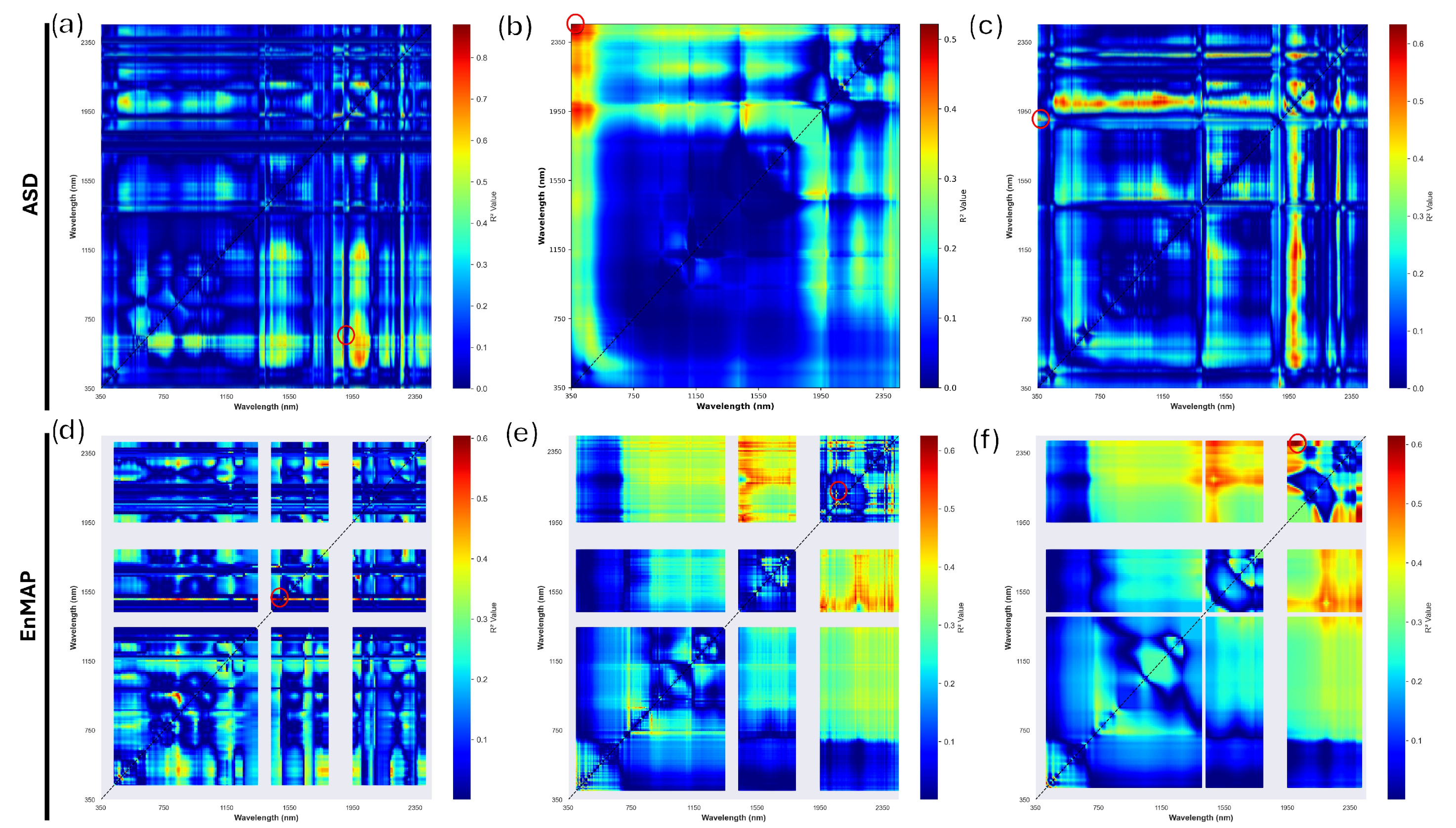
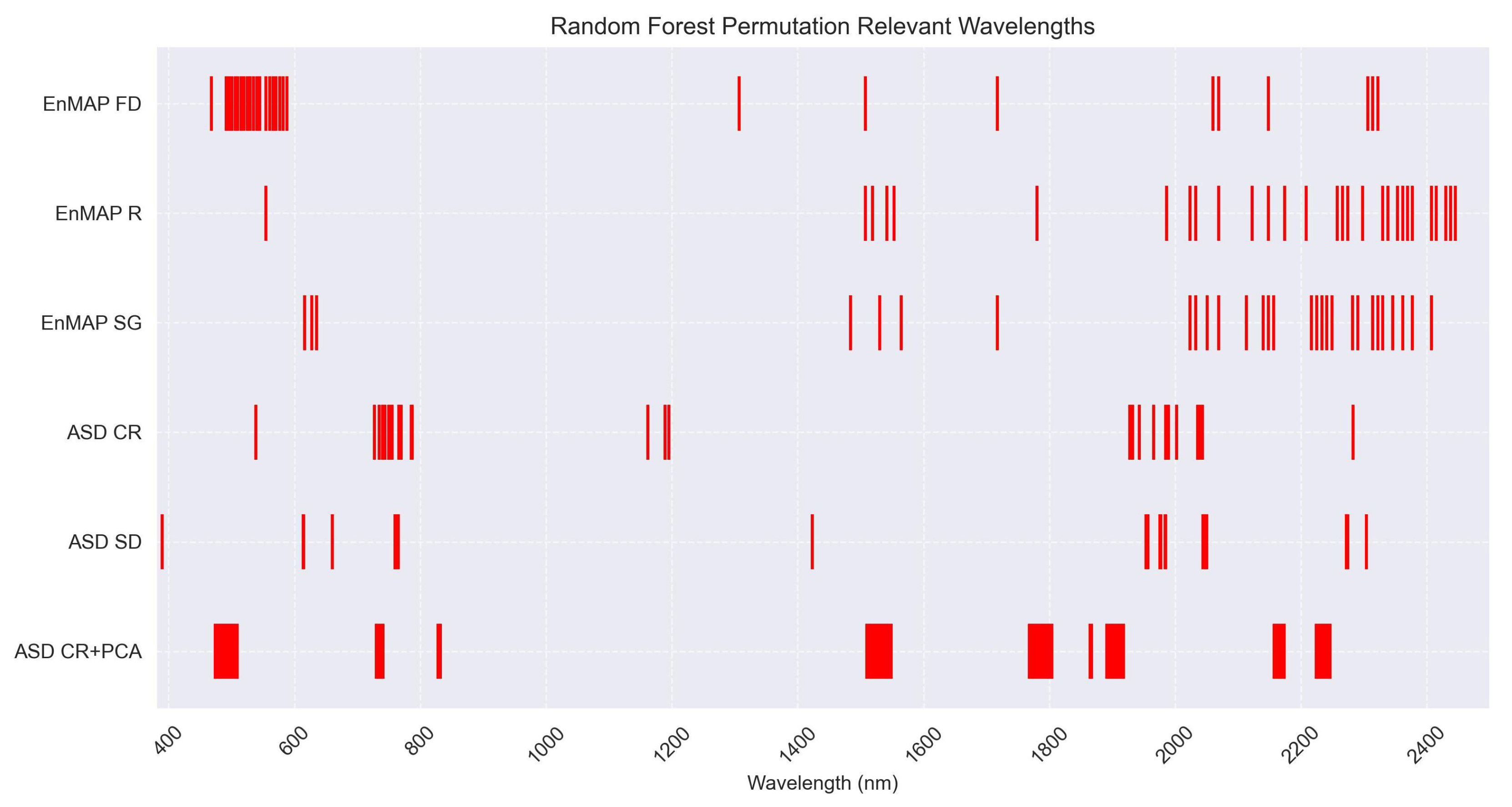
The aim of the study was to demonstrate and assess the capabilities of new-generation hyperspectral satellites, such as EnMAP, in detecting early stages of topsoil salinization. Concomitantly, we investigated the differences occurring between field and laboratory spectra to take into account their influence on model performance, projecting the so obtained results to the spaceborne-based analysis. To achieve this goal, laboratory-acquired spectra were first used to confirm that salinity-derived spectral modifications were detectable and that the models were capable of generalizing salt concentrations. The models tested provided satisfactory results regarding this prerequisite. For ASD laboratory-acquired data, more speditive models, such as 2D correlograms, proved to be an efficient tool in identifying the diagnostic spectral wavelengths (band pairs 1911–657 nm, 373–1910 nm, 382–2451 nm) that could be leveraged for quick mapping. On the other hand, PLSR did not provide the expected results. Otherwise, the Random Forest regressor proved to have a very good capability in capturing the ruling variables defining salinization-affected soils, with an $R^2$ of 0.74, RMSE of 0.98 dS/m and RPD of 1.89. The feasibility demonstrated by the analyses carried out on laboratory samples thereby provided a comparative benchmark for satellite analyses.

The models tested with the EnMAP-derived dataset produced similar results to those of ASD laboratory-acquired. PLSR proved to have very low performance, while 2D correlograms provided insights on useful wavelengths for salt detection (band pairs 1484–1518 nm, 2068–2130 nm, 2014–2407 nm). Concomitantly, the Random Forest regressor, upon deployment on the whole satellite image, proved to be the most efficient method, with $R^2$ of 0.60, RMSE of 0.61 dS/m and RPD of 1.57 for the SG dataset. The so obtained results testify to the model’s predictive capability for the detection of early stages of topsoil salinization.

It is important to acknowledge that the model performance is strongly influenced by the pre-processing treatment adopted. Additionally, the optimal technique differs depending on the considered dataset. Indeed, for laboratory spectra it was observed how CR + PCA transformation was beneficial to the model, reducing the number of spectral variables and enhancing absorption features. Similarly, for the satellite-derived dataset, the spectra shape was more influential for model regressive capabilities, therefore favouring transformations enhancing the spectra shape, such as FD, SD, SG filtering and, as a consequence of EnMAP’s extraordinary quality, reflectance itself. Aside from pre-processing parameter tuning, the best performing datasets are a manifestation of the spectral features observed in ASD and EnMAP spectra. In the former, salinization manifests as broad absorption features centred at 1400 and 1900 nm, also influencing the overall spectral reflectance of the sample. Conversely, for satellite-acquired datasets, the 1400 and 1900 nm ranges are not exploitable as they fall in the water vapour region. Nevertheless, spectral ranges 450–600 nm and 2000–2400 nm proved to be diagnostic wavelengths capable of detecting topsoil salinization. Overall, the generalization capabilities of the model were supported by the statistical analyses, showing how the demonstrative sample size can positively provide phenomena-related spectral modifications insights for both laboratory and spaceborne datasets.

In conclusion, further research should focus on the following:

• Validation of the predictions obtained with regression models: achievable with an increased sample size or deploying the trained model on an unobserved dataset containing field EC measurements for validation.
• Representativity of the field values in relation to satellite image pixels: addressable with a tighter and more extensive sampling grid capable of capturing the spatial variability of the phenomenon; differential weight assigned to field measure function of their position in the pixel, using the sensor’s Point Spread Function as a weight factor.
• Development of a multi-temporal analysis methodology for satellite-acquired hyperspectral data: beneficial for the definition of the spatio-temporal dynamics of the phenomenon but strongly related to model representativity and field sample collection for validation.

References

1. Patterson, L.A.; Lutz, B.; Doyle, M.W. Climate and Direct Human Contributions to Changes in Mean Annual Streamflow in the South Atlantic, USA. Water Resour. Res. 2013, 49, 7278–7291. [Google Scholar] [CrossRef]
2. Corwin, D.L. Climate Change Impacts on Soil Salinity in Agricultural Areas. Eur. J. Soil Sci. 2021, 72, 842–862. [Google Scholar] [CrossRef]
3. Commission, E. Consequences of Climate Change–European Commission. Available online: https://climate.ec.europa.eu/climate-change/consequences-climate-change_en (accessed on 25 March 2024).
4. van Dijk, M.; Morley, T.; Rau, M.L.; Saghai, Y. A meta-analysis of projected global food demand and population at risk of hunger for the period 2010–2050. Nat. Food 2021, 2, 494–501. [Google Scholar] [CrossRef] [PubMed]
5. Ivushkin, K.; Bartholomeus, H.; Bregt, A.K.; Pulatov, A.; Kempen, B.; De Sousa, L. Global Mapping of Soil Salinity Change. Remote Sens. Environ. 2019, 231, 111260. [Google Scholar] [CrossRef]
6. ASA; CSSA; SSSA. (Eds.) Alphabetical Listing of Soil Terms, A–Z; John Wiley & Sons, Ltd.: Hoboken, NJ, USA, 2008; pp. 1–75. [Google Scholar] [CrossRef]
7. Richards, L.A. Diagnosis and Improvement of Saline and Alkali Soils; U.S. Government Publishing Office: Washington, DC, USA, 1954; Volume 60. [Google Scholar]
8. Rengasamy, P. World Salinisation with Emphasis on Australia. Comp. Biochem. Phys. A 2005, 141, 337–348. [Google Scholar]
9. Eswar, D.; Karuppusamy, R.; Chellamuthu, S. Drivers of Soil Salinity and Their Correlation with Climate Change. Curr. Opin. Environ. Sustain. 2021, 50, 310–318. [Google Scholar] [CrossRef]
10. Metternicht, G.; Zinck, J.A. Remote Sensing of Soil Salinity: Potentials and Constraints. Remote Sens. Environ. 2003, 85, 1–20. [Google Scholar] [CrossRef]
11. Haubrock, S.; Chabrillat, S.; Kuhnert, M.; Hostert, P.; Kaufmann, H.J. Surface Soil Moisture Quantification and Validation Based on Hyperspectral Data and Field Measurements. J. Appl. Remote Sens. 2008, 2, 023552. [Google Scholar] [CrossRef]
12. Weiss, M.; Jacob, F.; Duveiller, G. Remote Sensing for Agricultural Applications: A Meta-Review. Remote Sens. Environ. 2020, 236, 111402. [Google Scholar] [CrossRef]
13. Jie, P.; Biswas, A.; Jiang, Q.; Zhao, R.; Jie, H.; Hu, J.; Hu, B.; Shi, Z. Estimating Soil Salinity from Remote Sensing and Terrain Data in Southern Xinjiang Province, China. Geoderma 2019, 337, 1309–1319. [Google Scholar] [CrossRef]
14. Bouaziz, M.; Matschullat, J.; Gloaguen, R. Improved Remote Sensing Detection of Soil Salinity from a Semi-Arid Climate in Northeast Brazil. Compt. Rendus Geosci. 2011, 343, 795–803. [Google Scholar] [CrossRef]
15. Fan, X.; Liu, Y.; Tao, J.; Weng, Y. Soil Salinity Retrieval from Advanced Multi-Spectral Sensor with Partial Least Square Regression. Remote Sens. 2015, 7, 488–511. [Google Scholar] [CrossRef]
16. Wang, L.; Zhang, B.; Shen, Q.; Yao, Y.; Zhang, S.; Wei, H.; Yao, R.; Zhang, Y. Estimation of Soil Salt and Ion Contents Based on Hyperspectral Remote Sensing Data: A Case Study of Baidunzi Basin, China. Water 2021, 13, 559. [Google Scholar] [CrossRef]
17. Wang, F.; Yang, S.; Wei, Y.; Shi, Q.; Ding, J. Characterizing Soil Salinity at Multiple Depth Using Electromagnetic Induction and Remote Sensing Data with Random Forests: A Case Study in Tarim River Basin of Southern Xinjiang, China. Sci. Total Environ. 2021, 754, 142030. [Google Scholar] [CrossRef]
18. Farifteh, J.; Farshad, A.; George, R.J. Assessing Salt-Affected Soils Using Remote Sensing, Solute Modelling, and Geophysics. Geoderma 2006, 130, 191–206. [Google Scholar] [CrossRef]
19. Farifteh, J.; van der Meer, F.; van der Meijde, M.; Atzberger, C. Spectral Characteristics of Salt-Affected Soils: A Laboratory Experiment. Geoderma 2008, 145, 196–206. [Google Scholar] [CrossRef]
20. Nawar, S.; Buddenbaum, H.; Hill, J. Estimation of Soil Salinity Using Three Quantitative Methods Based on Visible and Near-Infrared Reflectance Spectroscopy: A Case Study from Egypt. Arab. J. Geosci. 2015, 8, 5127–5140. [Google Scholar] [CrossRef]
21. Ghosh, G.; Kumar, S.; Saha, S.K. Hyperspectral Satellite Data in Mapping Salt-Affected Soils Using Linear Spectral Unmixing Analysis. J. Indian Soc. Remote Sens. 2012, 40, 129–136. [Google Scholar] [CrossRef]
22. Qian, T.; Tsunekawa, A.; Peng, F.; Masunaga, T.; Wang, T.; Li, R. Derivation of Salt Content in Salinized Soil from Hyperspectral Reflectance Data: A Case Study at Minqin Oasis, Northwest China. J. Arid Land 2019, 11, 111–122. [Google Scholar] [CrossRef]
23. Medhat Saleh, A.; Abd-Elwahed, M.; Metwally, Y.; Arafat, S. Capabilities of hyperspectral remote sensing data to detect soil salinity. Arab Univ. J. Agric. Sci. 2021, 29, 943–952. [Google Scholar] [CrossRef]
24. Hihi, S.; Rabah, Z.B.; Bouaziz, M.; Chtourou, M.Y.; Bouaziz, S. Prediction of Soil Salinity Using Remote Sensing Tools and Linear Regression Model. Adv. Remote Sens. 2019, 8, 77–88. [Google Scholar] [CrossRef]
25. Weng, Y.L.; Gong, P.; Zhu, Z.L. A Spectral Index for Estimating Soil Salinity in the Yellow River Delta Region of China Using EO-1 Hyperion Data. Pedosphere 2010, 20, 378–388. [Google Scholar] [CrossRef]
26. Loizzo, R.; Guarini, R.; Longo, F.; Scopa, T.; Formaro, R.; Facchinetti, C.; Varacalli, G. Prisma: The Italian Hyperspectral Mission. In Proceedings of the IGARSS 2018-2018 IEEE International Geoscience and Remote Sensing Symposium, Valencia, Spain, 22–27 July 2018; pp. 175–178. [Google Scholar] [CrossRef]
27. Guanter, L.; Kaufmann, H.; Segl, K.; Foerster, S.; Rogass, C.; Chabrillat, S.; Kuester, T.; Hollstein, A.; Rossner, G.; Chlebek, C.; et al. The EnMAP Spaceborne Imaging Spectroscopy Mission for Earth Observation. Remote Sens. 2015, 7, 8830–8857. [Google Scholar] [CrossRef]
28. Casa, R.; Tolomio, M.; Mzid, N.; Pignatti, S.; Pascucci, S. Estimation of Field Scale Topsoil Properties of Agronomic Interest from Prisma Imaging Spectrometer Data. In Proceedings of the 2021 IEEE International Geoscience and Remote Sensing Symposium IGARSS, Brussels, Belgium, 12–16 July 2021; pp. 480–483. [Google Scholar] [CrossRef]
29. Caramona, E.; Storch, T.; Chabrillat, S.; Wirth, K. Mission Quarterly Report 03 01.01.2023 to 31.03.2023; Technical Report 03; Deutsches Zentrum für Luft- und Raumfahrt (German Aerospace Center): Cologne, Germany, 2023. [Google Scholar]
30. Hunt, G.R.; Salisbury, J.W.; Lenhoff, C.J. Visible and Near-Infrared spectra of minerals and rocks: V. Halides, Phosphates, Arsenates, Vanadates and Borates. Mod. Geol. 1971, 3, 121–132. [Google Scholar]
31. Crowley, J.K. Visible and Near-Infrared (0.4–2.5 Mm) Reflectance Spectra of Playa Evaporite Minerals. J. Geophys. Res. Solid Earth 1991, 96, 16231–16240. [Google Scholar] [CrossRef]
32. Consorzio LaMMA. Climatologia di Grosseto 1991–2020. Available online: http://www.lamma.toscana.it/clima-e-energia/climatologia/clima-grosseto (accessed on 2 April 2024).
33. Bravetti, L.; Pranzini, G. L’evoluzione Quaternaria della pianura di Grosseto (Toscana): Prima interpretazione dei dati del sottosuolo. Geogr. Fis. Dinam. Quat. 1987, 10, 85–92. [Google Scholar]
34. Zanchi, C.; Cecchi, S. Soil Salinisation in the Grosseto Plain (Maremma, Italy): An Environmental and Socio-Economic Analysis of the Impact on the Agro-Ecosystem. In Coastal Water Bodies: Nature and Culture Conflicts in the Mediterranean; Scapini, F., Ciampi, G., Eds.; Springer: Dordrecht, The Netherlands, 2010; pp. 79–90. [Google Scholar] [CrossRef]
35. Falciai, M. Controllo Agronomico Delle Falde Saline in Zona Costiera: L’esempio Di Principina Terra. Univ. Florence 1996, 63. [Google Scholar]
36. Beemster, J.G.R.; Toscana, R. Soil and Groundwater Salinity in the Grosseto Plain and Its Implication for Irrigation. Univ. Amst. 1987. [Google Scholar]
37. Bencini, A.; Pranzini, G. The Salinization of Groundwaters in the Grosseto Plain (Tuscany, Italy); Dipartimento di scienze della terra, Università di Firenze: Florence, Italy, 1992. [Google Scholar]
38. Storch, T.; Chabrillat, S.; Wirth, K. Mission Quarterly Report 02 01.10.2022 to 31.12.2022; Technical Report 02; Deutsches Zentrum für Luft- und Raumfahrt (German Aerospace Center): Cologne, Germany, 2022. [Google Scholar]
39. DLR. EnMAP Product—00043167_31_2A_20230911T125456_010303_230922+U0BLNNTS330B. 2023. Available online: https://www.enmap.org/ (accessed on 22 September 2023).
40. DLR. EnMAP Product—0000043167_30_2A_20230911T125456_010400_231010+U0BLNNTS330B. 2023. Available online: https://www.enmap.org/ (accessed on 10 October 2023).
41. Malvern Panalytical. ASD FieldSpec 4-High Resolution Spectroradiometer|Malvern Panalytical. Available online: https://www.malvernpanalytical.com/en/products/product-range/asd-range/fieldspec-range/fieldspec4-hi-res-high-resolution-spectroradiometer (accessed on 8 March 2023).
42. FAO. Standard Operating Procedure for Soil Electrical Conductivity, Soil/Water, 1:5; Technical Report; FAO: Rome, Italy, 2021. [Google Scholar]
43. Instruments, X. 50110922 XS REVio Portable Multiparameter-Electrode 201 T-Polarographic Sensor. Available online: https://www.xsinstruments.com/it/product/50110922-xs-revio-portable-multiparameter-electrode-201-t-polarographic-sensor-without-cell (accessed on 1 July 2024).
44. Gholizadeh, A.; Neumann, C.; Chabrillat, S.; van Wesemael, B.; Castaldi, F.; Borůvka, L.; Sanderman, J.; Klement, A.; Hohmann, C. Soil Organic Carbon Estimation Using VNIR–SWIR Spectroscopy: The Effect of Multiple Sensors and Scanning Conditions. Soil Tillage Res. 2021, 211, 105017. [Google Scholar] [CrossRef]
45. Ben Dor, E.; Ong, C.; Lau, I.C. Reflectance Measurements of Soils in the Laboratory: Standards and Protocols. Geoderma 2015, 245–246, 112–124. [Google Scholar] [CrossRef]
46. Savitzky, A.; Golay, M.J.E. Smoothing and Differentiation of Data by Simplified Least Squares Procedures. Anal. Chem. 1964, 36, 1627–1639. [Google Scholar] [CrossRef]
47. Vestergaard, R.J.; Vasava, H.B.; Aspinall, D.; Chen, S.; Gillespie, A.; Adamchuk, V.; Biswas, A. Evaluation of Optimized Preprocessing and Modeling Algorithms for Prediction of Soil Properties Using VIS-NIR Spectroscopy. Sensors 2021, 21, 6745. [Google Scholar] [CrossRef] [PubMed]
48. Clark, R.N.; Roush, T.L. Reflectance Spectroscopy: Quantitative Analysis Techniques for Remote Sensing Applications. J. Geophys. Res. Solid Earth 1984, 89, 6329–6340. [Google Scholar] [CrossRef]
49. Chang, C.W.; Laird, D.A.; Mausbach, M.J.; Hurburgh, C.R. Near-Infrared Reflectance Spectroscopy–Principal Components Regression Analyses of Soil Properties. Soil Sci. Soc. Am. J. 2001, 65, 480–490. [Google Scholar] [CrossRef]
50. Hopkins, D.W. What Is a Norris Derivative? NIR News 2001, 12, 3–5. [Google Scholar] [CrossRef]
51. Draper, N.R.; Smith, H. Applied Regression Analysis; John Wiley & Sons: Hoboken, NJ, USA, 1998. [Google Scholar]
52. Montgomery, D.C.; Runger, G.C. Applied Statistics and Probability for Engineers; John Wiley & Sons: Hoboken, NJ, USA, 2010. [Google Scholar]
53. Wang, S.; Chen, Y.; Wang, M.; Li, J. Performance Comparison of Machine Learning Algorithms for Estimating the Soil Salinity of Salt-Affected Soil Using Field Spectral Data. Remote Sens. 2019, 11, 2605. [Google Scholar] [CrossRef]
54. Ward, K.J.; Chabrillat, S.; Brell, M.; Castaldi, F.; Spengler, D.; Foerster, S. Mapping Soil Organic Carbon for Airborne and Simulated EnMAP Imagery Using the LUCAS Soil Database and a Local PLSR. Remote Sens. 2020, 12, 3451. [Google Scholar] [CrossRef]
55. Stenberg, B.; Viscarra Rossel, R.A.; Mouazen, A.M.; Wetterlind, J. Chapter Five-Visible and Near Infrared Spectroscopy in Soil Science. In Advances in Agronomy; Sparks, D.L., Ed.; Academic Press: Cambridge, MA, USA, 2010; Volume 107, pp. 163–215. [Google Scholar] [CrossRef]
56. Minasny, B.; McBratney, A.B. Regression Rules as a Tool for Predicting Soil Properties from Infrared Reflectance Spectroscopy. Chemom. Intell. Lab. Syst. 2008, 94, 72–79. [Google Scholar] [CrossRef]
57. Pedregosa, F.; Varoquaux, G.; Gramfort, A.; Michel, V.; Thirion, B.; Grisel, O.; Blondel, M.; Prettenhofer, P.; Weiss, R.; Dubourg, V.; et al. Scikit-Learn: Machine Learning in Python. Mach. Learn. Python 2011, 12, 2825–2830. [Google Scholar]
58. Sidike, A.; Zhao, S.; Wen, Y. Estimating Soil Salinity in Pingluo County of China Using QuickBird Data and Soil Reflectance Spectra. Int. J. Appl. Earth Obs. Geoinf. 2014, 26, 156–175. [Google Scholar] [CrossRef]
59. Wang, Q.; Li, P.; Chen, X. Modeling Salinity Effects on Soil Reflectance under Various Moisture Conditions and Its Inverse Application: A Laboratory Experiment. Geoderma 2012, 170, 103–111. [Google Scholar] [CrossRef]
60. Liu, Y.; Pan, X.; Wang, C.; Li, Y.; Shi, R. Predicting Soil Salinity with Vis–NIR Spectra after Removing the Effects of Soil Moisture Using External Parameter Orthogonalization. PLoS ONE 2015, 10, e0140688. [Google Scholar] [CrossRef]
61. Thompson, D.R.; Guanter, L.; Berk, A.; Gao, B.C.; Richter, R.; Schläpfer, D.; Thome, K.J. Retrieval of Atmospheric Parameters and Surface Reflectance from Visible and Shortwave Infrared Imaging Spectroscopy Data. Surv. Geophys. 2019, 40, 333–360. [Google Scholar] [CrossRef]
62. Weng, Y.; Gong, P.; Zhu, Z. Reflectance Spectroscopy for the Assessment of Soil Salt Content in Soils of the Yellow River Delta of China. Int. J. Remote Sens. 2008, 29, 5511–5531. [Google Scholar] [CrossRef]
63. Srivastava, R.; Sethi, M.; Yadav, R.K.; Bundela, D.S.; Singh, M.; Chattaraj, S.; Singh, S.K.; Nasre, R.A.; Bishnoi, S.R.; Dhale, S.; et al. Visible-Near Infrared Reflectance Spectroscopy for Rapid Characterization of Salt-Affected Soil in the Indo-Gangetic Plains of Haryana, India. J. Indian Soc. Remote Sens. 2017, 45, 307–315. [Google Scholar] [CrossRef]
64. Escribano, P.; Schmid, T.; Chabrillat, S.; Rodríguez-Caballero, E.; García, M. Optical Remote Sensing for Soil Mapping and Monitoring; Elsevier Inc.: Amsterdam, The Netherlands, 2017; pp. 87–125. [Google Scholar] [CrossRef]
65. García-Soria, J.L.; Morata, M.; Berger, K.; Pascual-Venteo, A.B.; Rivera-Caicedo, J.P.; Verrelst, J. Evaluating epistemic uncertainty estimation strategies in vegetation trait retrieval using hybrid models and imaging spectroscopy data. Remote Sens. Environ. 2024, 310, 114228. [Google Scholar] [CrossRef]
66. Morata, M.; Siegmann, B.; Pérez-Suay, A.; García-Soria, J.L.; Rivera-Caicedo, J.P.; Verrelst, J. Neural Network Emulation of Synthetic Hyperspectral Sentinel-2-Like Imagery With Uncertainty. IEEE J. Sel. Top. Appl. Earth Obs. Remote Sens. 2023, 16, 762–772. [Google Scholar] [CrossRef]
Figure 3. ASD laboratory measurements of samples with different salinity levels. The non-saline sample has the highest reflectance (blue spectra), with the strongly-saline sample having the lowest (green spectra). It is also possible to appreciate the absorption features centred at 1400 and 1900 nm.
Remotesensing 17 02486 g003
Figure 4. EnMAP-derived pixel spectra bounding the field sampling sites. It is possible to observe the contribution to the pixel spectra of multiple features such as dry vegetation, with bare soil being the prevalent component.
Remotesensing 17 02486 g004
Figure 5. Distribution of EC values for the field-collected samples represented according to the salinity classes defined by Richards [7].
Remotesensing 17 02486 g005
Figure 6. Representation of the best two-dimensional correlogram derived indexes, Computed for the ASD (ac) and EnMAP (df) datasets. (a) FD ratio index; (b) R ratio index; (c) FD difference index; (d) FD ratio index; (e) R ratio index; (f) SG ratio index. The colour gradient blue-to-red represents the R 2 value for the bands represented on the X and Y axes of the graphs. Red circles represent the bands with highest statistical significance.
Remotesensing 17 02486 g006
Figure 7. RF regression plots for the ASD (ac) and EnMAP (df) datasets. (a) CR+PCA; (b) CR; (c) SD; (d) SG; (e) R; (f) FD. Dashed line represents the identity line ( y = x ), red line is the fitted regression line, blue points represent the sample’s EC values.
Remotesensing 17 02486 g007
Figure 8. Distribution of EC values for the EnMAP-derived spectral signatures represented according to the salinity classes defined by Richards [7].
Remotesensing 17 02486 g008
Figure 9. Computation of the best index–wavelength combination, RI-SG ( S G 2014 , S G 2407 ), on the whole EnMAP scene [39,40]. The low variability in EC values highlights the index’s inability to capture spectral differences among image pixels. This insight further supports the observation that a simple combination of two spectral bands is insufficient to detect and map current levels of salinization.
Remotesensing 17 02486 g009
Figure 10. Deployment of the Random Forest regressor on the whole EnMAP scene. Model trained on the extracted pixel spectral signatures and field EC values [39,40]. The blue-to-red colour gradient represents progressively increasing EC values for bare soil pixels. The variability in these values, combined with field knowledge, validates the model’s predictions.
Remotesensing 17 02486 g010
Figure 11. Random Forest permutation results representing the diagnostic wavelengths for the most relevant datasets of both EnMAP pixel-derived spectra and ASD laboratory-acquired spectra.
Remotesensing 17 02486 g011