
Seasonally Robust Offshore Wind Turbine Detection in Sentinel-2 Imagery Using Imaging Geometry-Aware Deep Learning

Abstract

1. Introduction
2. Study Area and Datasets
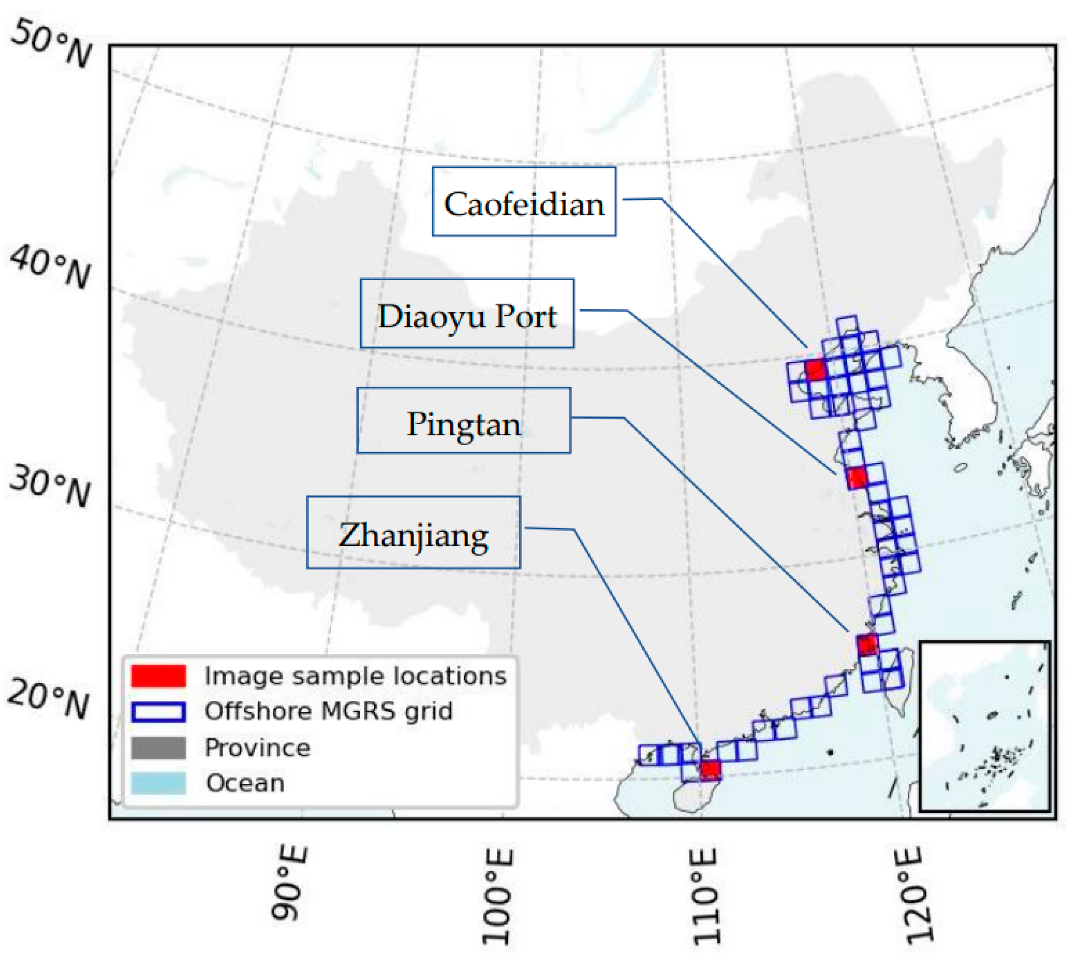
2.1. Study Area
2.2. Datasets
2.2.1. Offshore Wind Turbines
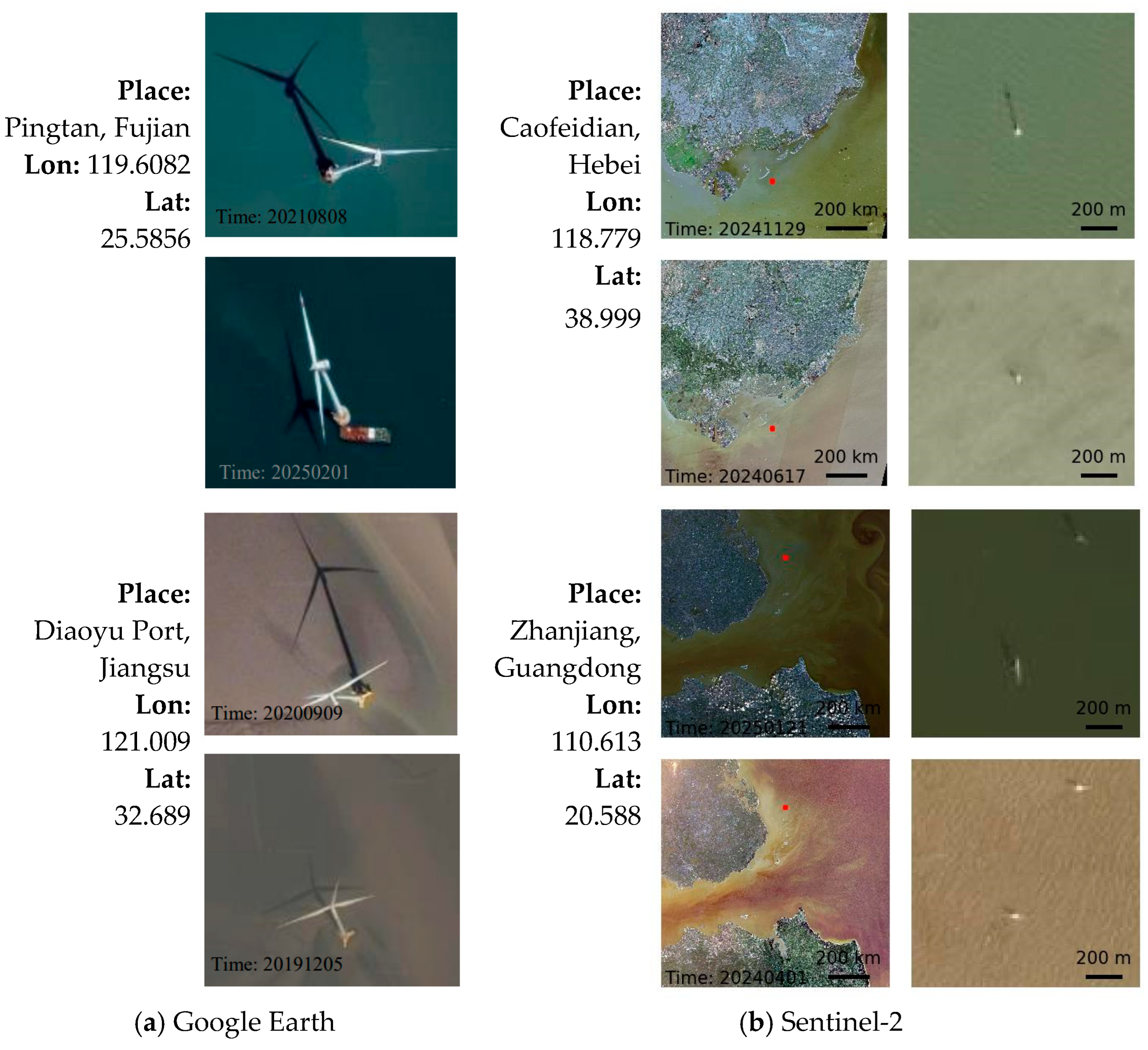
2.2.2. Sentinel-2 Imagery
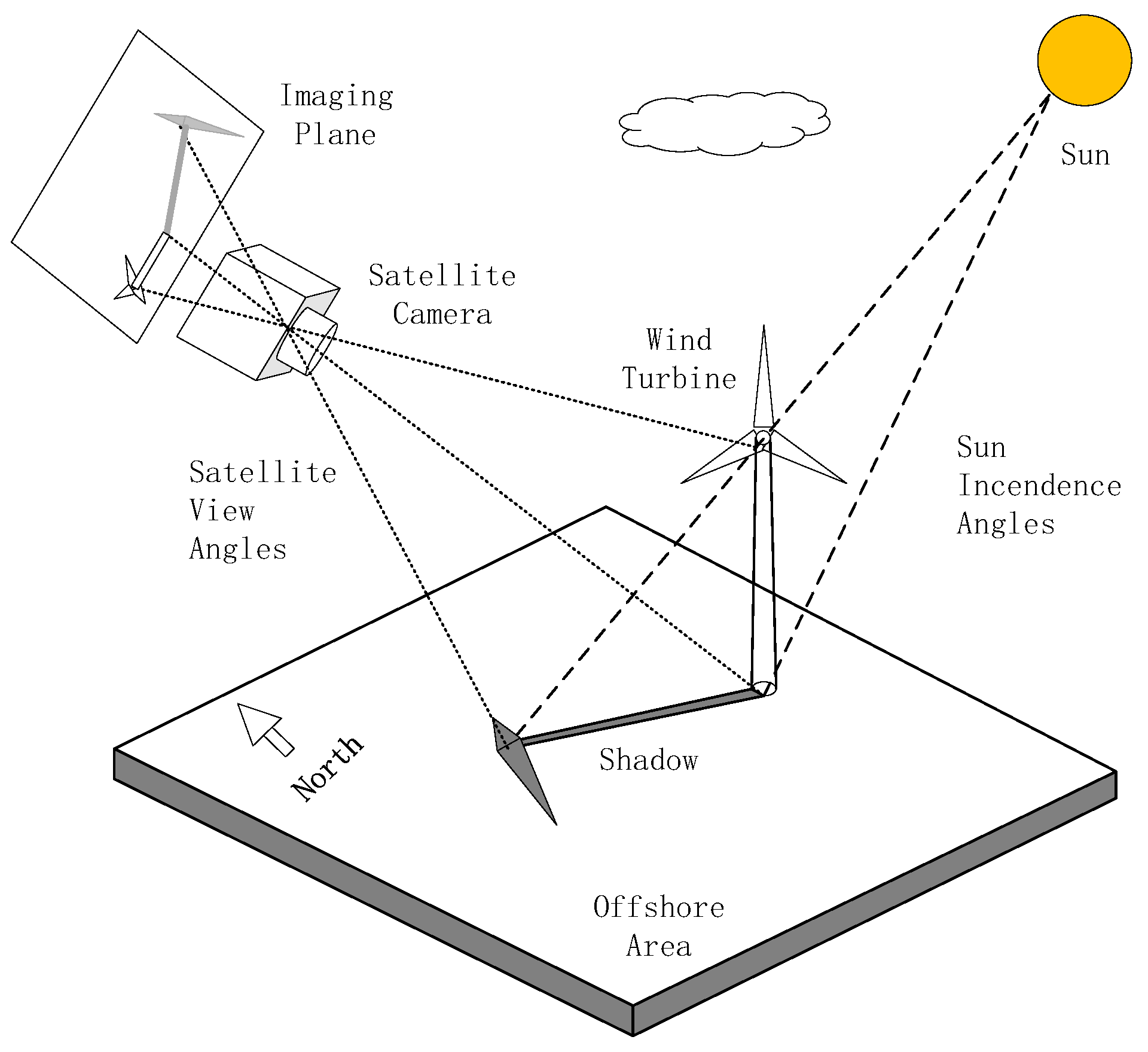
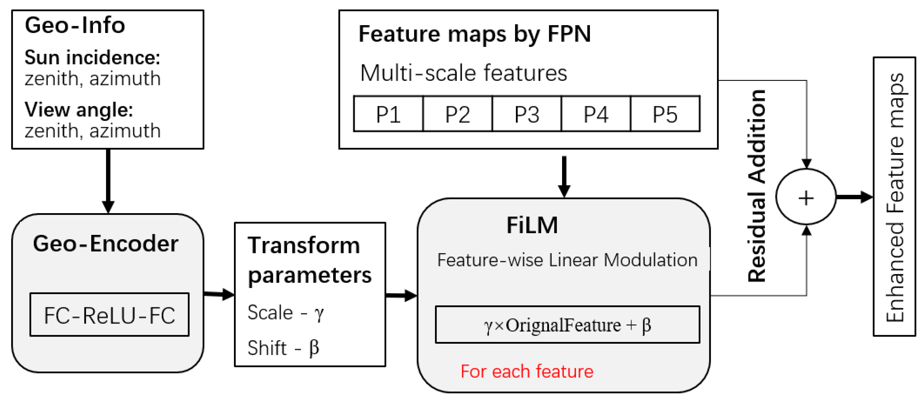
2.2.3. Imaging Geometry Metadata
2.2.4. OWT Samples
3. Methods
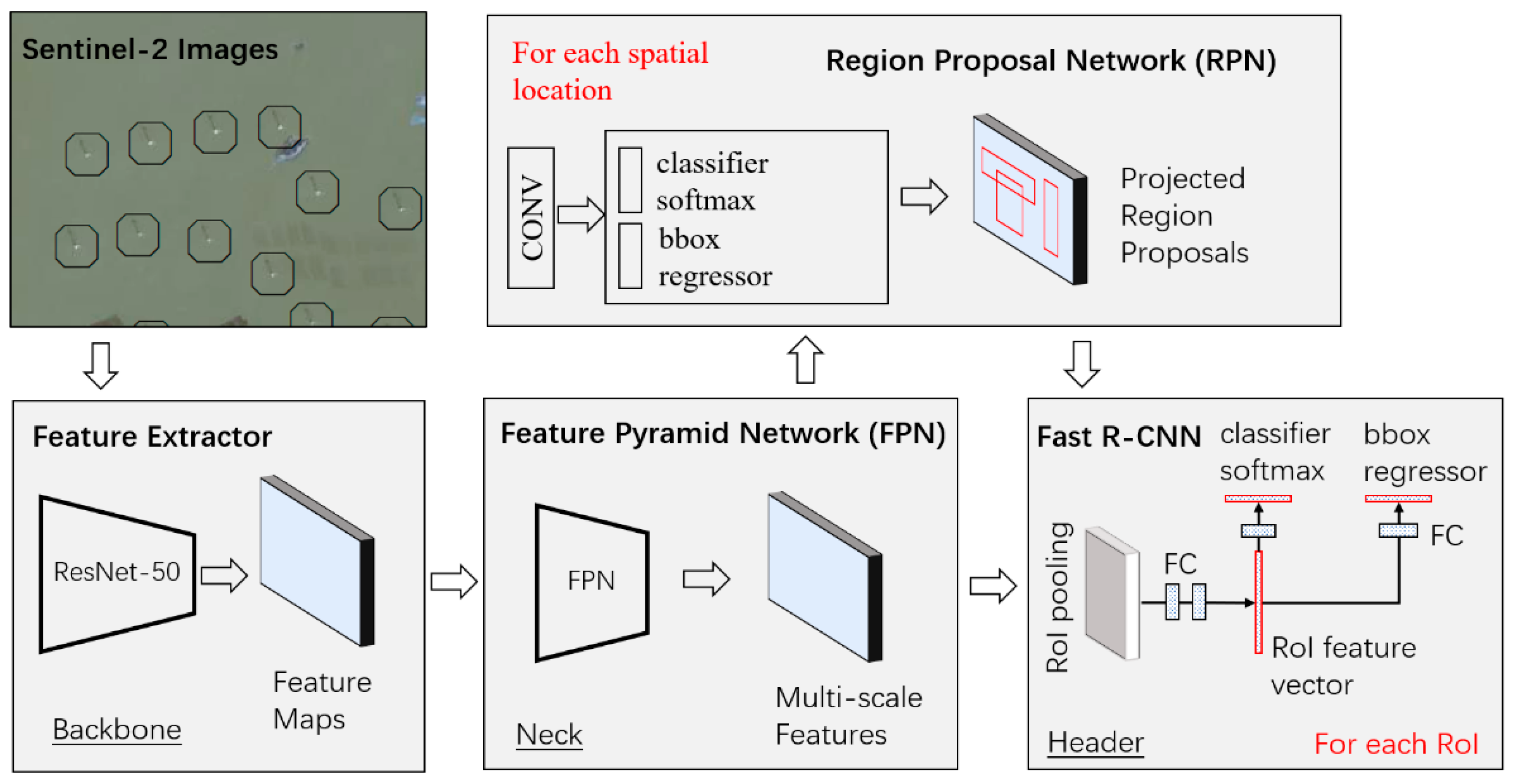
3.1. Model Design
3.1.1. Geowise-Net
3.1.2. Contrast-Net
- Positive and negative image pair selection: Two images from the same geographic location but at different times are treated as positive pairs, while images from nearby but distinct locations are treated as negative pairs. This setup enables the model to learn turbine representations that are invariant to seasonal, illumination, and shadow-related changes by maximizing feature similarity in positive pairs and dissimilarity in negative pairs.
- Feature extraction and comparison: After passing the image pairs through the backbone and FPN, contrastive learning is applied to feature maps from levels P2 to P5, which correspond to small, medium, and large scales. The highest-resolution layer, P1, is excluded due to its dominance of low level texture and details, which may hinder temporal feature alignment. For each selected level, the similarity between feature representations of image pairs, either positive or negative, is computed to guide the learning process.
- Contrastive loss computation: Contrastive loss is a loss function used in deep learning to learn representations that bring positive pairs (augmentations of the similar images) closer together while pushing all other images (negatives) apart in the embedding space. The loss function of Information Noise-Contrastive Estimation (InfoNCE) from the Simple Framework for Contrastive Learning of Visual Representations (SimCLR) is adopted as follows:
- Given an image pair (xi, xj), with their features denoted as (zi, zj), the cosine similarity of the two features at the layer (l) can be calculated as follows:where denotes the lth feature, .
3.1.3. Composite Model
3.2. Experimental Design
3.2.1. Construction of OWT Training and Testing Samples
3.2.2. Model Training and Evaluation
4. Results
4.1. Quantitative Evaluation
4.1.1. Evaluation with Bounding Boxes of OWT Samples
4.1.2. Evaluation with OWT Sample Points
4.2. The Impact of Seasonal Variation on OWT Detection
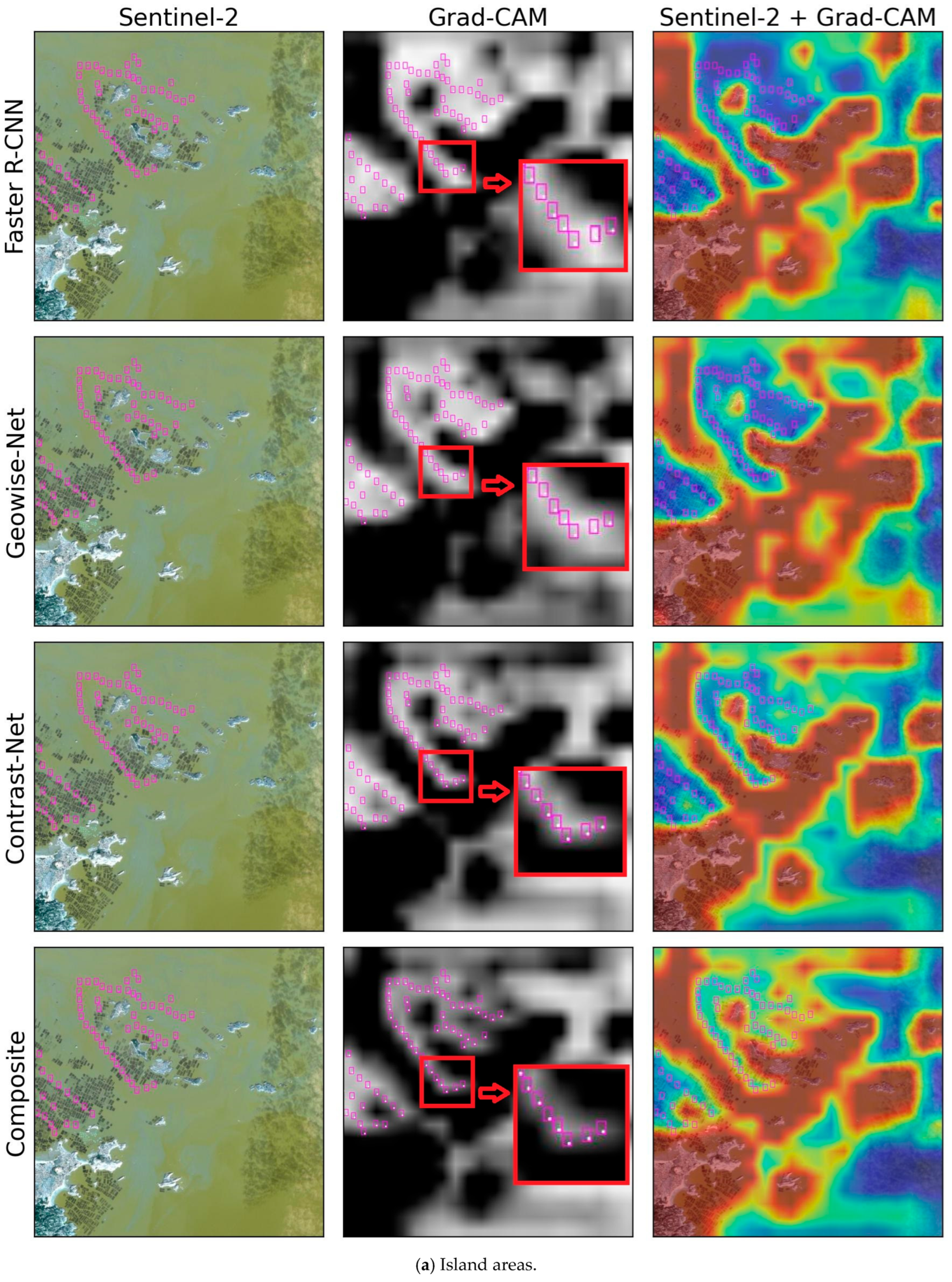
4.3. Grad-CAM Highlight of OWT Features
4.4. Multi-Temporal OWT Mapping
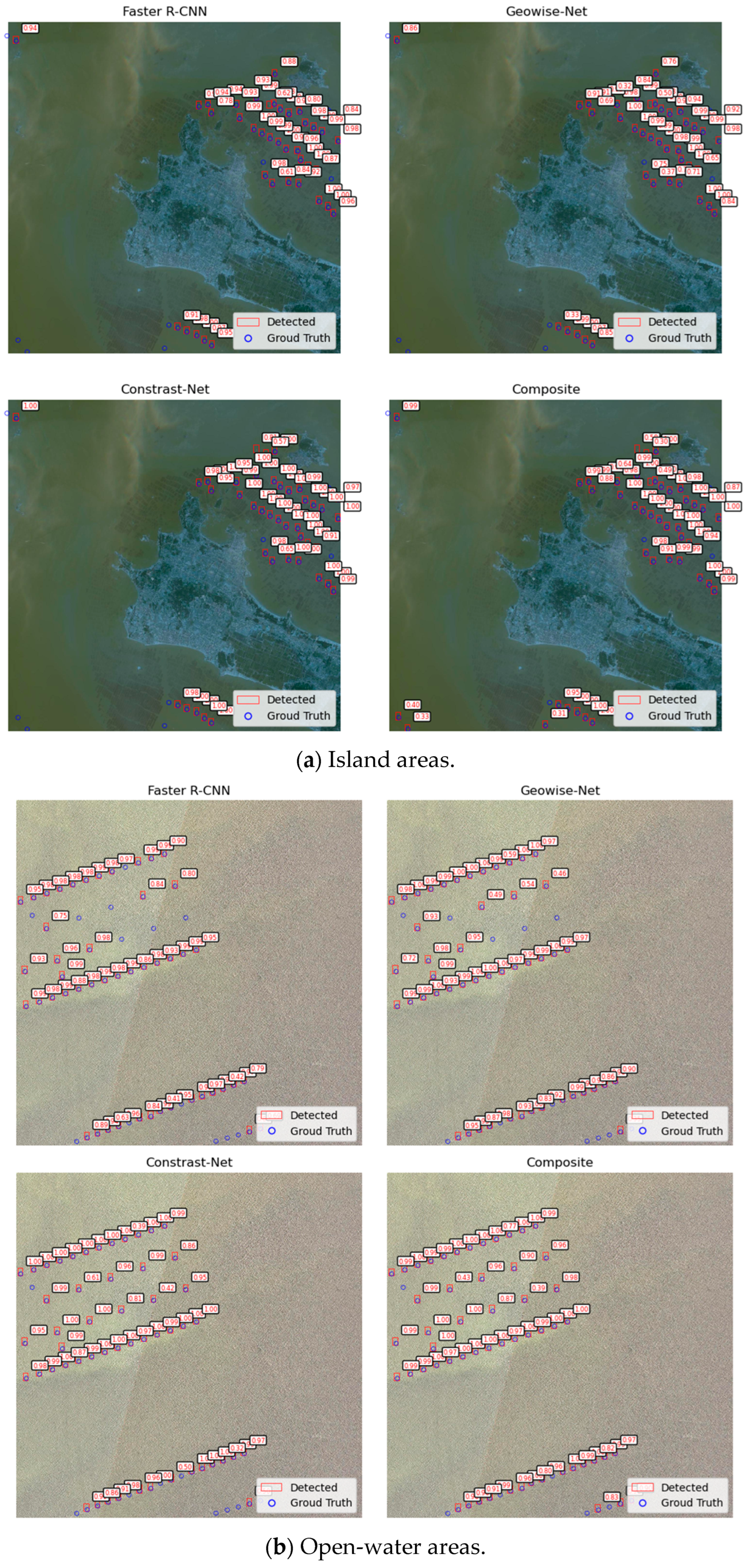
4.4.1. Visualization of Single-Scene Detection
4.4.2. Generation of Unified OWT Dataset from Multi-Seasonal Sentinel-2 Imagery
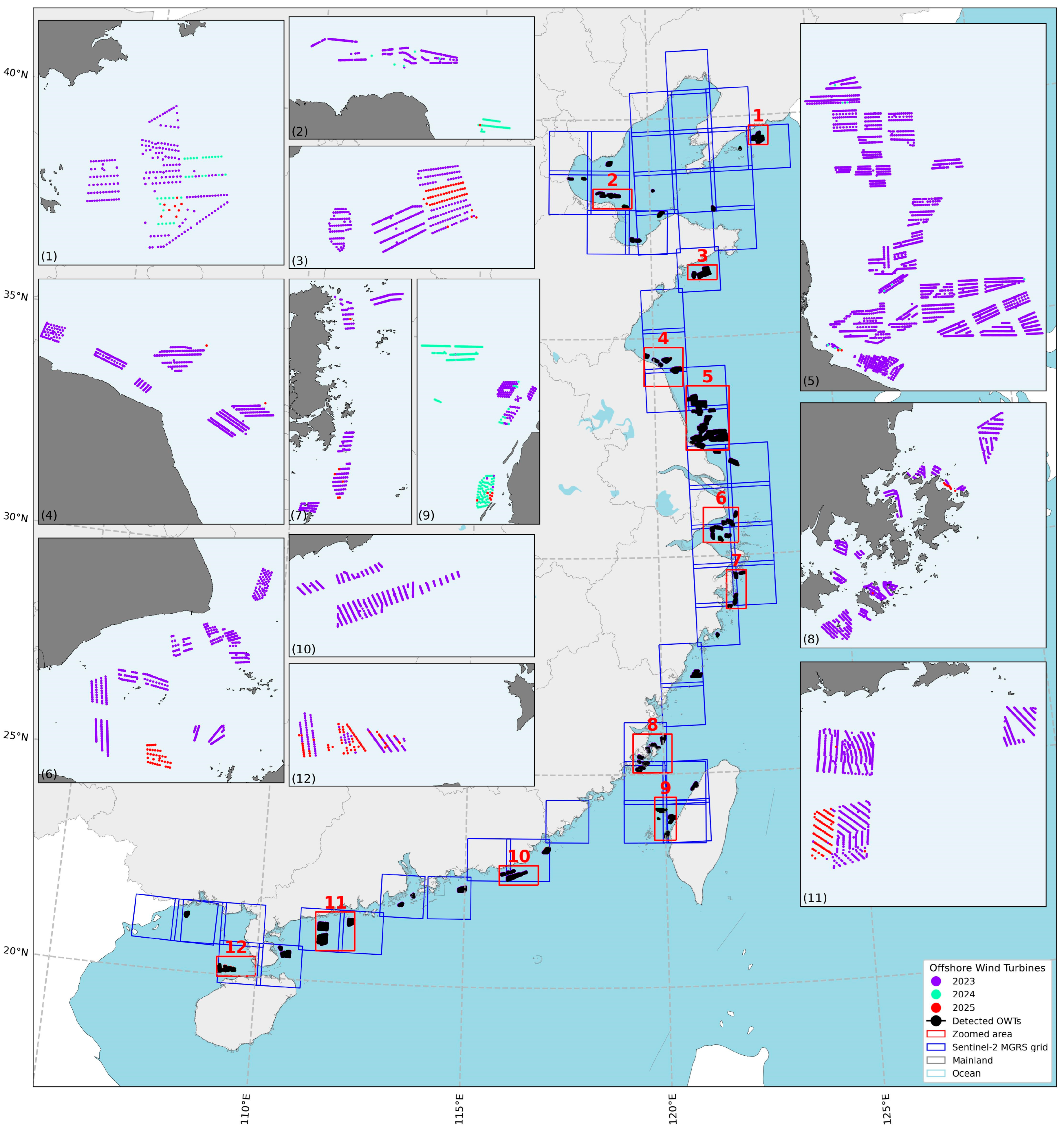
4.4.3. Mapping of China Offshore Wind Turbine Dataset
5. Discussion
6. Conclusions
Author Contributions
Funding
Data Availability Statement
Acknowledgments
Conflicts of Interest
Abbreviations
| OWT | Offshore Wind Turbine |
| GW | Gigawatt |
| ESA | European Space Agency |
| MGRS | Military Grid Reference System |
| UTM | Universal Transverse Mercator |
| MLP | Multilayer Perceptron |
| FC | Fully Connected |
| CNN | Convolutional Neural Network |
| ReLU | Rectified Linear Unit |
| FPN | Feature Pyramid Network |
| RPN | Region Proposal Network |
| ROI | Region of Interest |
| FiLM | Feature-wise Linear Modulation |
| Grad-CAM | Gradient-weighted Class Activation Mapping |
| InfoNCE | Information Noise-Contrastive Estimation |
| SimCLR | Simple Framework for Contrastive Learning of Visual Representation |
| IoU | Intersection over Union |
| AP | Average Precision |
| AR | Average Recall |
| TP | True Positive |
| FP | False Positive |
| FN | False Negative |
| SOTA | State of the Art |
References
- Bilgili, M.; Alphan, H. Technological and dimensional improvements in onshore commercial large-scale wind turbines in the world and Turkey. Clean Technol. Environ. Policy 2023, 25, 3303–3317. [Google Scholar] [CrossRef]
- Bilgili, M.; Alphan, H. Global growth in offshore wind turbine technology. Clean Technol. Environ. Policy 2022, 24, 2215–2227. [Google Scholar] [CrossRef]
- Zhang, T.; Tian, B.; Sengupta, D.; Zhang, L.; Si, Y. Global offshore wind turbine dataset. Sci. Data 2021, 8, 191. [Google Scholar] [CrossRef] [PubMed]
- Dunnett, S.; Sorichetta, A.; Taylor, G.; Eigenbrod, F. Harmonised global datasets of wind and solar farm locations and power. Sci. Data 2020, 7, 130. [Google Scholar] [CrossRef] [PubMed]
- Hoeser, T.; Feuerstein, S.; Kuenzer, C. DeepOWT: A global offshore wind turbine data set derived with deep learning from Sentinel-1 data. Earth Syst. Sci. Data 2022, 14, 4251–4270. [Google Scholar] [CrossRef]
- Wang, K.; Xiao, W.; He, T.; Zhang, M. Remote sensing unveils the explosive growth of global offshore wind turbines. Renew. Sustain. Energy Rev. 2024, 191, 114186. [Google Scholar] [CrossRef]
- Marino, A.; Velotto, D.; Nunziata, F. Offshore Metallic Platforms Observation Using Dual-Polarimetric TS-X/TD-X Satellite Imagery: A Case Study in the Gulf of Mexico. IEEE J. Sel. Top. Appl. Earth Obs. Remote Sens. 2017, 10, 4376–4386. [Google Scholar] [CrossRef]
- Wong, B.A.; Thomas, C.; Halpin, P. Automating offshore infrastructure extractions using synthetic aperture radar & Google Earth Engine. Remote Sens. Environ. 2019, 233, 111412. [Google Scholar]
- He, T.; Hu, Y.; Li, F.; Chen, Y.; Zhang, M.; Zheng, Q.; Jin, Y.; Ren, H. Mapping land- and offshore-based wind turbines in China in 2023 with Sentinel-2 satellite data. Renew. Sustain. Energy Rev. 2025, 214, 115566. [Google Scholar] [CrossRef]
- Kang, M.; Ji, K.; Leng, X.; Lin, Z. Contextual Region-Based Convolutional Neural Network with Multilayer Fusion for SAR Ship Detection. Remote Sens. 2017, 9, 860. [Google Scholar] [CrossRef]
- Berwo, M.A.; Khan, A.; Fang, Y.; Fahim, H.; Javaid, S.; Mahmood, J.; Abideen, Z.U.; Syam, M.S. Deep Learning Techniques for Vehicle Detection and Classification from Images/Videos: A Survey. Sensors 2023, 23, 4832. [Google Scholar] [CrossRef] [PubMed]
- Yildirim, E.; Kavzoglu, T. Deep convolutional neural networks for ship detection using refined DOTA and TGRS-HRRSD high-resolution image datasets. Adv. Space Res. 2025, 75, 1871–1887. [Google Scholar] [CrossRef]
- Liu, S.; Kong, W.; Chen, X.; Xu, M.; Yasir, M.; Zhao, L.; Li, J. Multi-Scale Ship Detection Algorithm Based on a Lightweight Neural Network for Spaceborne SAR Images. Remote Sens. 2022, 14, 1149. [Google Scholar] [CrossRef]
- Lu, Z.; Wang, P.; Li, Y.; Ding, B. A New Deep Neural Network Based on SwinT-FRM-ShipNet for SAR Ship Detection in Complex Near-Shore and Offshore Environments. Remote Sens. 2023, 15, 5780. [Google Scholar] [CrossRef]
- Zhai, Y.; Chen, X.; Cao, X.; Cui, X. Identifying wind turbines from multiresolution and multibackground remote sensing imagery. Int. J. Appl. Earth Obs. Geoinf. 2024, 126, 103613. [Google Scholar] [CrossRef]
- Liu, L.; Wu, M.; Zhao, J.; Bing, L.; Zheng, L.; Luan, S.; Mao, Y.; Xue, M.; Liu, J.; Liu, B. Deep learning-based monitoring of offshore wind turbines in Shandong Sea of China and their location analysis. J. Clean. Prod. 2024, 434, 140415. [Google Scholar] [CrossRef]
- Manso-Callejo, M.-Á.; Cira, C.-I.; Alcarria, R.; Arranz-Justel, J.-J. Optimizing the Recognition and Feature Extraction of Wind Turbines through Hybrid Semantic Segmentation Architectures. Remote Sens. 2020, 12, 3743. [Google Scholar] [CrossRef]
- Xie, J.; Tian, T.; Hu, R.; Yang, X.; Xu, Y.; Zan, L. A Novel Detector for Wind Turbines in Wide-Ranging, Multiscene Remote Sensing Images. IEEE J. Sel. Top. Appl. Earth Obs. Remote Sens. 2024, 17, 17725–17738. [Google Scholar] [CrossRef]
- Sun, G.; Huang, H.; Weng, Q.; Zhang, A.; Jia, X.; Ren, J.; Sun, L.; Chen, X. Combinational shadow index for building shadow extraction in urban areas from Sentinel-2A MSI imagery. Int. J. Appl. Earth Obs. Geoinf. 2019, 78, 53–65. [Google Scholar] [CrossRef]
- Mandroux, N.; Dagobert, T.; Drouyer, S.; von Gioi, R.G. Single Date Wind Turbine Detection on Sentinel-2 Optical Images. Image Process. Line 2022, 12, 198–217. [Google Scholar] [CrossRef]
- Zhang, S.; He, Y.; Gu, Y.; He, Y.; Wang, H.; Wang, H.; Yang, R.; Chady, T.; Zhou, B. UAV based defect detection and fault diagnosis for static and rotating wind turbine blade: A review. Nondestruct. Test. Eval. 2024, 40, 1691–1729. [Google Scholar] [CrossRef]
- Zhou, G.; Song, C.; Simmers, J.; Cheng, P. Urban 3D GIS From LiDAR and digital aerial images. Comput. Geosci. 2004, 30, 345–353. [Google Scholar] [CrossRef]
- Fraser, C.S. Network Design Considerations for Non-Metric Cameras. Photogramm. Eng. Remote Sens. 1984, 50, 1115–1126. [Google Scholar]
- Deng, Z.; Sun, H.; Zhou, S.; Zhao, J.; Lei, L.; Zou, H. Multi-scale object detection in remote sensing imagery with convolutional neural networks. ISPRS J. Photogramm. Remote Sens. 2018, 145, 3–22. [Google Scholar] [CrossRef]
- Ren, S.; He, K.; Girshick, R.; Sun, J. Faster R-CNN: Towards Real-Time Object Detection with Region Proposal Networks. arXiv 2015, arXiv:1506.01497. [Google Scholar] [CrossRef] [PubMed]
- Sammani, F.; Joukovsky, B.; Deligiannis, N. Visualizing and Understanding Contrastive Learning. arXiv 2022, arXiv:2206.09753v3. [Google Scholar] [CrossRef] [PubMed]


| Model | Precision | Recall | F1 Score |
|---|---|---|---|
| Faster R-CNN | 0.955 | 0.944 | 0.947 |
| Geowise-Net | 0.971 | 0.947 | 0.958 |
| Contrast-Net | 0.976 | 0.949 | 0.961 |
| Composite | 0.981 | 0.953 | 0.966 |
| Model | Precision | Recall | F1 Score |
|---|---|---|---|
| Faster R-CNN | 0.970 | 0.948 | 0.957 |
| Geowise-Net | 0.978 | 0.951 | 0.963 |
| Contrast-Net | 0.981 | 0.952 | 0.965 |
| Composite | 0.984 | 0.954 | 0.968 |
| Model | Precision | Recall | F1 Score |
|---|---|---|---|
| Faster R-CNN | 0.918 | 0.932 | 0.920 |
| Geowise-Net | 0.953 | 0.938 | 0.944 |
| Contrast-Net | 0.961 | 0.943 | 0.950 |
| Composite | 0.974 | 0.948 | 0.960 |
| Model | Precision | Recall | F1 Score |
|---|---|---|---|
| Faster R-CNN | 0.977 | 0.925 | 0.951 |
| Geowise-Net | 0.990 | 0.933 | 0.961 |
| Contrast-Net | 0.992 | 0.935 | 0.962 |
| Composite | 0.994 | 0.936 | 0.964 |
Disclaimer/Publisher’s Note: The statements, opinions and data contained in all publications are solely those of the individual author(s) and contributor(s) and not of MDPI and/or the editor(s). MDPI and/or the editor(s) disclaim responsibility for any injury to people or property resulting from any ideas, methods, instructions or products referred to in the content. |
© 2025 by the authors. Licensee MDPI, Basel, Switzerland. This article is an open access article distributed under the terms and conditions of the Creative Commons Attribution (CC BY) license (https://creativecommons.org/licenses/by/4.0/).
Share and Cite
Song, X.; Li, Z. Seasonally Robust Offshore Wind Turbine Detection in Sentinel-2 Imagery Using Imaging Geometry-Aware Deep Learning. Remote Sens. 2025, 17, 2482. https://doi.org/10.3390/rs17142482
Song X, Li Z. Seasonally Robust Offshore Wind Turbine Detection in Sentinel-2 Imagery Using Imaging Geometry-Aware Deep Learning. Remote Sensing. 2025; 17(14):2482. https://doi.org/10.3390/rs17142482
Chicago/Turabian StyleSong, Xike, and Ziyang Li. 2025. "Seasonally Robust Offshore Wind Turbine Detection in Sentinel-2 Imagery Using Imaging Geometry-Aware Deep Learning" Remote Sensing 17, no. 14: 2482. https://doi.org/10.3390/rs17142482
APA StyleSong, X., & Li, Z. (2025). Seasonally Robust Offshore Wind Turbine Detection in Sentinel-2 Imagery Using Imaging Geometry-Aware Deep Learning. Remote Sensing, 17(14), 2482. https://doi.org/10.3390/rs17142482