CropSTS: A Remote Sensing Foundation Model for Cropland Classification with Decoupled Spatiotemporal Attention

Abstract

Recent progress in geospatial foundation models (GFMs) has demonstrated strong generalization capabilities for remote sensing downstream tasks. However, existing GFMs still struggle with fine-grained cropland classification due to ambiguous field boundaries, insufficient and low-efficient temporal modeling, and limited cross-regional adaptability. In this paper, we propose CropSTS, a remote sensing foundation model designed with a decoupled temporal–spatial attention architecture, specifically tailored for the temporal dynamics of cropland remote sensing data. To efficiently pre-train the model under limited labeled data, we employ a hybrid framework combining joint-embedding predictive architecture with knowledge distillation from web-scale foundation models. Despite being trained on a small dataset and using a compact model, CropSTS achieves state-of-the-art performance on the PASTIS-R benchmark in terms of mIoU and F1-score. Our results validate that structural optimization for temporal encoding and cross-modal knowledge transfer constitute effective strategies for advancing GFM design in agricultural remote sensing.

1. Introduction

Fine-grained cropland classification is a fundamental task in precision agriculture and land-use monitoring [1,2,3], which faces unique challenges stemming from the inherent complexity of agricultural ecosystems, including region-specific cultivation practices, cultural influences on land-use patterns, and dynamic interactions with climatic conditions. While supervised deep learning has driven progress in remote sensing analytics, the emerging paradigm of geospatial foundation models (GFMs) presents a transformative approach. Trained through self-supervised learning on petabyte-scale multimodal satellite data [4], GFMs overcome critical limitations of annotation-dependent methods by capturing universal representations of geospatial semantics. Their capability to adapt knowledge across heterogeneous regions and downstream tasks (e.g., crop type mapping, phenology monitoring) [2,5] positions GFMs as a scalable framework for agricultural intelligence, particularly in data-scarce or annotation-constrained scenarios.

However, current remote sensing foundation models [6,7] often overlook or treat temporal information in a simplistic manner, which limits their effectiveness in cropland classification tasks. In remote sensing data, temporal dynamics represent a crucial yet relatively independent dimension. Existing models primarily focus on single-date imagery, neglecting the rich temporal patterns essential for understanding crop growth cycles. Despite the growing popularity of geospatial foundation models (GFMs) for Earth observation tasks, most existing models primarily focus on spatial feature extraction, while temporal information is often handled in an rudimentary manner—e.g., by concatenating or averaging multitemporal inputs without dedicated temporal modeling. This limits their ability to effectively capture dynamic patterns and phenological changes that are critical in remote sensing applications such as crop monitoring, land-use change detection, and seasonal variation analysis [8]. Some approaches attempt to incorporate temporal information through post hoc stacking or feature fusion [9,10,11,12], showing marginal improvements. However, such methods still fail to capture deep phenological cues embedded in temporal sequences.

Unlike natural video data, where objects move and spatial positions change over time, necessitating joint spatiotemporal modeling, remote sensing imagery presents a unique scenario. In remote sensing, the spatial coordinates of observed areas remain fixed across temporal sequences, while the temporal dimension captures variations in spectral signatures due to factors like phenological changes, agricultural practices, or environmental conditions. This inherent characteristic suggests that spatial and temporal information in remote sensing data can be effectively modeled separately [13]. By decoupling spatial and temporal features, models can more precisely capture the distinct patterns present in each dimension, leading to improved performance in tasks such as land cover classification and change detection.

Accurate delineation of farmland boundaries is crucial for agricultural monitoring, land management, and precision farming. These boundaries often share semantic relationships with adjacent land features, such as roads, water bodies, or forested areas. While unsupervised learning methods have shown promise in extracting features of various land cover types from remote sensing imagery [14], they typically lack the capacity to specifically model the relationships between farmland parcels and their surrounding features. However, the availability of open-source platforms like OpenStreetMap (OSM) provides an opportunity to incorporate prior knowledge of land boundaries into the learning process [15]. By integrating OSM data, it becomes feasible to guide unsupervised models to better capture the contextual and semantic associations between farmland and neighboring land cover types, thereby enhancing the precision of boundary extraction.

To address these challenges, we propose CropSTS, a computation-efficient geospatial foundation model with a decoupled spatiotemporal transformer architecture. Unlike existing monolithic designs, CropSTS introduces a decoupled spatial–temporal attention pathway with temporal-first design, enabling more effective encoding of crop phenology before spatial aggregation. CropSTS is, to the best of our knowledge, the first remote sensing model designed for agricultural field classification that adopts a time-first decoupled attention structure while maintaining computational efficiency. The model is pre-trained using a hybrid framework that integrates joint-embedding predictive architecture with cross-model knowledge distillation from a large ViT backbone. Notably, CropSTS achieves state-of-the-art results on the PASTIS-R dataset under low-data regimes, demonstrating superior performance in both accuracy and generalization with significantly reduced model complexity.

In summary, our key contributions are as follows:

• We introduce CropSTS, the first compute-efficient GFM designed with a temporally decoupled attention structure for remote sensing cropland classification.
• We develop a hybrid training strategy combining joint-embedding predictive architecture and knowledge distillation, enabling efficient model transfer from vision-scale pre-trained backbones to agricultural domains, as well as the enhancement of cropland boundary delineation.
• We empirically validate the effectiveness of our approach on the PASTIS-R benchmark, achieving strong performance under limited training and data settings.

2. Related Work

2.1. Vision Transformers in Remote Sensing

The adaptation of vision transformers (ViTs) to remote sensing has evolved through three waves of innovation. Vision transformers (ViTs) [16] fundamentally redefined remote sensing analysis by replacing convolutional inductive biases with pure attention mechanisms, enabling unified processing of multimodal satellite data through spectral-agnostic tokenization, as well as a strong ability of scaling expansion. Early attempts [4,17] directly transplanted ViT architectures, simply extending positional encodings to accommodate multispectral bands (e.g., SatViT’s wavelength-aware positional biases). Subsequent works [18,19] introduced temporal extensions, processing multi-date inputs via factorized spacetime attention (e.g., TimeSformer-RS). While these adaptations improved cross-task generalization over CNNs, they inherit two core limitations from natural image paradigms: (i) global self-attention tends to smear localized phenological patterns critical for crop discrimination, as evidenced by the 22% performance drop on fragmented fields in AgriBench [20]; (ii) fixed spectral–temporal tokenization disrupts the intrinsic spatiotemporal disentanglement in farming landscapes, particularly failing to distinguish spectrally homologous fields under different irrigation regimes [21]. Recent efforts to incorporate local window attention [22] partially mitigate these issues but at the cost of losing global crop rotation context.

2.2. Geospatial Foundation Models

The evolution of remote sensing foundation models (RSFMs) has undergone three transformative phases, driven by architectural innovation and scaling laws. Initial efforts repurposed vision transformers (ViTs) for multispectral analysis through band-specific positional encoding (e.g., SatViT [23]), achieving moderate cross-task transferability. The breakthrough emerged with geospatial-adapted self-supervised paradigms: masked image modeling (e.g., GeoMAE with spectral-aware masking [6]) and multitemporal contrastive learning (e.g., seasonal contrast [24]), enabling pre-training on ${10}^7$ km² satellite imagery. Current state-of-the-art GFMs integrate hybrid architectures—cascading CNN-ViT backbones for multi-resolution fusion, coupled with spatiotemporal tokenizers that disentangle phenological cycles from structural patterns (e.g., P²FEViT [25], CMTNet [26]). This progression demonstrates a paradigm shift: from naively transplanting natural image architectures to developing geophysical inductive biases, and ultimately achieving modality-aware pre-training at continental scales, with model capacity scaling from 100M to 10B+ parameters. Crucially, each leap correlates with improvements in few-shot mapping accuracy while reducing annotation costs [27,28].

2.3. Self-Supervised Learning

Self-supervised learning (SSL) in remote sensing predominantly follows three pathways [24,29], each with distinct advantages and limitations for agricultural foundation models, as shown in

Table 1. Types and characteristics of self-supervised learning methods.

Method Type	Principle	Representative Methods
Contrastive Learning	Learning from positive and negative sample pairs	SimCLR [30], MoCo [31], BYOL [32]
Masked Image Modeling	Reconstructing masked information	MAE [33], BEiT [34], SimMIM [35]
Generative Self-Supervised Learning	Autoencoder architecture	Autoencoder [36], VAE [37], GAN [38]
Non-Contrastive Learning	Constructing guiding models	VICReg [39], DINO [40]

.

As a teacher–student framework, DINO uniquely satisfies two key requirements for agricultural GFMs [40]. Though native DINO enforces temporal invariance, its decoupled teacher–student structure provides an ideal substrate for injecting phenological awareness—our key innovation. Unlike MAE [33], which focuses on low-level spectral reconstruction, DINO yields semantically rich and transferable features, better suited for cross-region cropland representation. Its architecture inherently maintains spatial consistency while allowing flexible adaptation through its momentum-driven teacher design. Though vanilla DINO promotes temporal invariance, its decoupled structure forms an ideal backbone for injecting phenological sensitivity—our core innovation. In contrast to forecasting-oriented models, such as Next2Sat [41], DINO scales robustly with data and model size [42], making it a principled and scalable foundation for learning fine-grained spatiotemporal patterns in agriculture.

To enhance object-level feature learning, we adopt the Object-Aware DINO (Oh-A-DINO) framework [43], which extends the self-supervised DINO model [40] by integrating fine-grained object-centric representations. Oh-A-DINO first applies PCA to the DINO patch embeddings to segment salient foreground objects, and then encodes these segments using a variational autoencoder (VAE) to extract object-specific latent vectors. These vectors are concatenated with the global DINO representations, yielding a unified feature space that captures both holistic scene context and detailed object attributes. This hybrid design improves the model’s ability to distinguish between objects with similar shapes but different colors or materials—an essential capability for fine-grained classification tasks, such as cropland boundary delineation. Compared to traditional slot-based approaches [44] and object-centric diffusion models [45], Oh-A-DINO achieves improved object-level discrimination while avoiding the need for full model retraining. It also builds upon the strong generalization capabilities of vision transformers like DINO and its successors [46].

2.4. Knowledge Distillation in Earth Observation

Knowledge distillation has proven effective in adapting large-scale vision models to geospatial tasks by transferring learned feature hierarchies from general-purpose teachers to domain-specific student models. The core hypothesis is that visual semantic priors (e.g., texture patterns, object boundaries) pre-trained on natural images (e.g., ImageNet) exhibit transferable representations for Earth observation, which can be refined with limited labeled geospatial data. Studies demonstrate that vision foundation models (VFMs) like ViT and ConvNeXt provide strong initialization for geospatial tasks. ViT-Base pre-trained on ImageNet achieves 68.4% accuracy on EuroSAT land cover classification [47]. Feature hierarchies from early layers capture universal edge/texture patterns, while deeper layers encode task-specific semantics [3]. KD-based compression retains teacher model accuracy on crop mapping while reducing parameters [48]. The transferability stems from shared low-level visual cues between natural and geospatial imagery. This congruence enables VFMs to serve as universal feature extractors, with KD fine-tuning them toward geospatial specificity.

2.5. Current Limitations

While existing ViT-based methods have demonstrated strong performance in remote sensing tasks, they typically treat spatial and temporal features in a coupled or flattened manner. This design often dilutes phenological signals essential for crop-type discrimination, particularly in fine-grained agricultural landscapes. In addition, most self-supervised learning (SSL) methods in remote sensing emphasize pixel-level reconstruction or contrastive objectives on static imagery, overlooking temporal dynamics critical to seasonal crop monitoring. Recent advances in vision foundation models, particularly those trained on large-scale natural image datasets, have shown promising transferability to geospatial domains. These models encode rich semantic priors and robust visual patterns that can serve as a strong initialization for downstream remote sensing tasks. When appropriately adapted, such pre-trained models can significantly improve performance, especially under limited supervision, by transferring generalized knowledge while being fine-tuned to capture domain-specific temporal and spectral characteristics.

3. Method

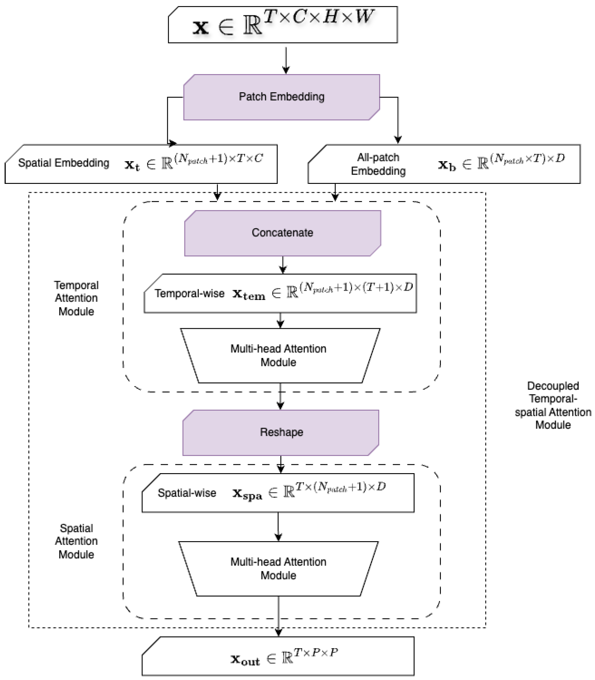
3.1. Model Architecture

CropSTS adopts a ViT-S backbone with a decoupled encoder design: a temporal attention module is first applied across the time dimension, followed by spatial attention over individual patches. This allows more efficient and interpretable modeling of crop phenology. The overall structure is shown in Figure 1.

Given an input tensor $x\in {\mathbb{R}}^{b\times c\times t\times h\times w}$ representing multitemporal Sentinel-2 patches (batch size b, channels c, time steps t, height h, width w), we first compute patch embeddings as follows:

$$z^{\left(0\right)}=\mathrm{Linear}\left(\mathrm{Flatten}\left(x\right)\right)+P_t+P_s$$

(1)

where $P_t\in {\mathbb{R}}^{t\times d}$ and $P_s\in {\mathbb{R}}^{(h\times w)\times d}$ denote learnable temporal and spatial positional encodings, respectively.

3.1.1. Decoupled Temporal–Spatial Attention Mechanism

Let $z^{\left(l\right)}\in {\mathbb{R}}^{N\times C}$ denote the input token sequence at the l-th attention layer, where N is the number of tokens (temporal or spatial) and C is the feature dimension. In both temporal and spatial attention blocks, we adopt the standard scaled dot-product attention. Specifically, for any input z, the attention computation consists of the following steps:

$$\widehat{z}=\mathrm{LayerNorm}\left(z\right),Q=\widehat{z}{W}_q,K=\widehat{z}{W}_k,V=\widehat{z}{W}_v,$$

(2)

$$A=\mathrm{Softmax}\left({\displaystyle \frac{Q{K}^T}{\sqrt{d/k}}}\right),z^{(l+1)}=z+\gamma AV,$$

(3)

where $W_q$, $W_k$, and $W_v\in {\mathbb{R}}^{C\times C}$ are learnable projection matrices for query, key, and value, respectively. The scaling factor $\gamma$ is a learnable scalar that adaptively modulates the strength of the attention output at each layer.

In our architecture, we decouple temporal and spatial attention to better capture field-specific phenological dynamics and spatial structure. The attention is applied in two sequential stages:

Temporal Attention. Given the input feature sequence $z_t^{\left(l\right)}$ across T time steps, we apply temporal attention to extract temporally coherent features:

$${\widehat{z}}_t^{\left(l\right)}=\mathrm{LayerNorm}(z_t^{\left(l\right)}),Q_t={\widehat{z}}_t^{\left(l\right)}{W}_q^t,K_t={\widehat{z}}_t^{\left(l\right)}{W}_k^t,V_t={\widehat{z}}_t^{\left(l\right)}{W}_v^t,$$

(4)

$$A_t=\mathrm{Softmax}\left({\displaystyle \frac{Q_t{K}_t^T}{\sqrt{d/k}}}\right),z_t^{(l+1)}=z_t^{\left(l\right)}+{\gamma }_t{A}_t{V}_t,$$

(5)

Spatial Attention. We then apply spatial attention to the temporally aggregated representation $z_t^{(l+1)}$, focusing on spatial relationships within each timestamp:

$${\widehat{z}}_s^{\left(l\right)}=\mathrm{LayerNorm}(z_t^{(l+1)}),Q_s={\widehat{z}}_s^{\left(l\right)}{W}_q^s,K_s={\widehat{z}}_s^{\left(l\right)}{W}_k^s,V_s={\widehat{z}}_s^{\left(l\right)}{W}_v^s,$$

(6)

$$A_s=\mathrm{Softmax}\left({\displaystyle \frac{Q_s{K}_s^T}{\sqrt{d/k}}}\right),z_s^{(l+1)}=z_t^{(l+1)}+{\gamma }_s{A}_s{V}_s,$$

(7)

The learnable scaling coefficients ${\gamma }_t$ and ${\gamma }_s$ are designed to allow the model to flexibly adjust the relative influence of temporal and spatial attention at each layer. This design enables the model to dynamically emphasize either temporal dependencies or spatial context based on the input data characteristics and learning dynamics. The structure of the decoupled temporal–spatial attention mechanism is shown in Figure 2. The pseudo-code is shown in Algorithm 1.

Algorithm 1 Spatial–temporal alternating processing.

Require: Input sequence $x\in {\mathbb{R}}^{b\times c\times t\times h\times w}$   1: Compute patch embeddings $z^{\left(0\right)}$ with positional encodings   2: for $l=1$ to L do                ▹ Temporal attention across time   3:       Reshape $z^{(l-1)}$ to ${\mathbb{R}}^{(b\times hw)\times t\times d}$   4:       Compute temporal attention $A_t$ via Equation (2)   5:       Update: $z_t=z^{(l-1)}+A_t$                       ▹ Spatial attention within each frame   6:       Reshape $z_t$ to ${\mathbb{R}}^{(b\times t)\times hw\times d}$   7:       Compute spatial attention $A_s$ via Equation (3)   8:       Update: $z^{\left(l\right)}=z_t+A_s$   9: end for 10: return Final representation $z^{\left(L\right)}$

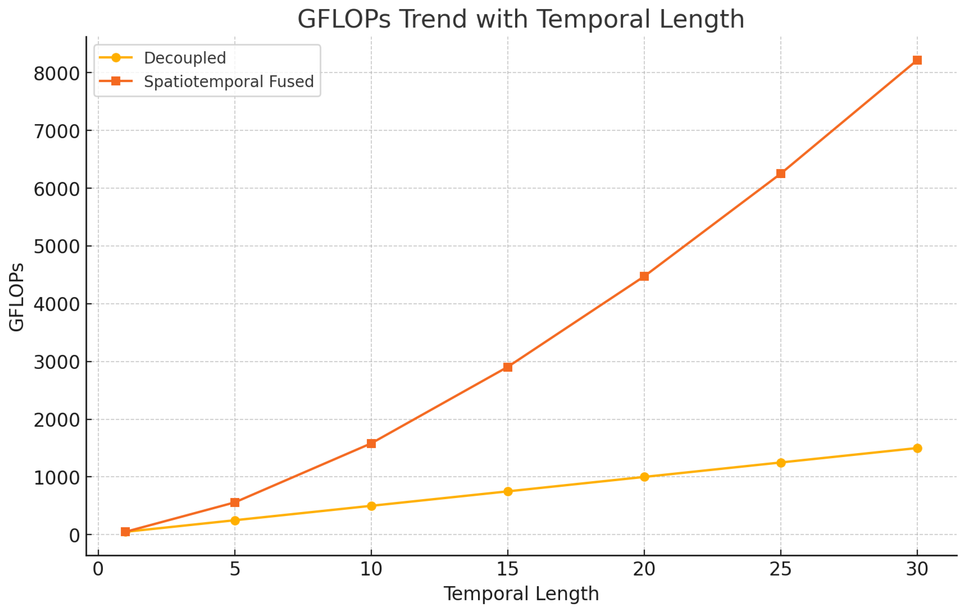
3.1.2. Complexity Analysis

In contrast to joint spatiotemporal attention, which incurs a computational complexity of $O\left(t^2{h}^2{w}^{2}d\right)$, our decoupled approach significantly reduces the cost to

$$O(L·[t^{2}d+h^2{w}^{2}d])$$

(8)

Under typical agricultural settings ($t=15$, $h=16$, $w=16$, $d=384$), this design achieves a 16× reduction in FLOPs (23.4 GFLOPs vs. 379.2 GFLOPs), demonstrating the scalability of our model for large-scale Earth observation.

3.2. Self-Supervised Learning

We adopt DINO, a non-contrastive self-distillation framework, as the backbone of our pre-training strategy. DINO consists of a student network $f_s$ updated via backpropagation and a teacher network $f_t$ updated by exponential moving average (EMA) of the student’s weights:

$${\theta }_t\leftarrow \lambda {\theta }_t+(1-\lambda ){\theta }_s$$

(9)

To enhance boundary learning in cropland segmentation, we introduce a tailored input masking strategy:

-

The student network receives partially masked inputs, where cropland regions are selectively occluded using plot-wise masks.

-

The teacher network receives the full, unmasked input.

This asymmetric view enforces the model to infer cropland boundaries and interior semantics from incomplete visual cues, encouraging sensitivity to spatial transitions and subtle edge signals, which is a critical aspect for accurate field boundary detection.

Given an input sequence $x\in {\mathbb{R}}^{c\times t\times h\times w}$, we generate N views ${\left\{x_i\right\}}_{i=1}^N$, where some student views are randomly masked using cropland segmentation masks $M\in {\{0,1\}}^{t\times h\times w}$. To generate the N views used in DINO training, we apply a set of diverse data augmentations—including random cropping, flipping, color jittering, and Gaussian blurring—to the same input image, following the multi-crop strategy proposed in [40]. These transformations result in a combination of two global views (covering larger regions) and several local views (smaller patches), which are processed differently by the teacher and student networks. The learning objective aligns student and teacher outputs across views via cross-view KL divergence:

$${\mathcal{L}}_{\mathrm{DINO}}=\sum _{i\ne j}\mathrm{KL}\left(f_t(x_i^{\mathrm{full}})\Vert f_s(x_j^{\mathrm{masked}})\right)$$

(10)

This spatially aware masking strategy transforms DINO into a object-centric pre-training paradigm, encouraging the encoder to reason about occluded regions and to learn structured semantic priors that align with cropland parcel shapes. Specifically, we retain more pixels near cropland boundaries and mask central homogeneous regions, which pushes the student to reconstruct the more uncertain or structurally informative parts. As a result, the model becomes more sensitive to fine-grained spatial transitions and learns to encode sharper object boundaries.

3.3. Knowledge Distillation

To complement temporal modeling with static visual priors, we introduce a cross-modal distillation loss that transfers knowledge from a large RGB-pre-trained teacher model, DINOv1 [40]. DINO v1 with ViT-B/16 is a self-supervised vision transformer model trained without labels using a student–teacher framework. It takes image patches (16 × 16) as input and outputs dense visual features from the final transformer layer. The model was pre-trained on ImageNet-1K using multi-crop augmentations and shows strong performance in transfer learning tasks. Despite the lack of supervision, it learns semantically meaningful representations that align well with object boundaries and classes, enabling competitive results on classification and segmentation benchmarks. The student network receives multitemporal inputs, while the teacher processes only the central RGB frame. Let $x_i\in {\mathbb{R}}^d$ and $y_i\in {\mathbb{R}}^d$ denote the student and teacher feature vectors for the i-th patch. We define the alignment loss as

$${\mathcal{L}}_{\mathrm{align}}={\displaystyle \frac{1}{n}}\sum _{i=1}^n{∥x_i-y_i∥}_2^{\alpha }$$

(11)

We use $\alpha =2$ and apply $L_2$ normalization to both $x_i$ and $y_i$ prior to loss computation. This encourages the student to mimic the teacher’s spatial feature geometry while preserving temporal reasoning.

The final training loss is a weighted combination of the DINO self-distillation loss and the cross-modal alignment loss:

$${\mathcal{L}}_{\mathrm{total}}={\mathcal{L}}_{\mathrm{DINO}}+{\lambda }_{\mathrm{align}}·{\mathcal{L}}_{\mathrm{align}}$$

(12)

This hybrid supervision strategy leverages both temporal consistency from unlabeled sequences and transferable spatial priors from large RGB models, enabling robust and generalizable pre-training under limited labels.

4. Results and Discussion

4.1. Experimental Setup

We evaluate our proposed CropSTS model on the PASTIS-R dataset, a standardized benchmark for cropland segmentation and classification in remote sensing. PASTIS-R consists of 2433 multitemporal image patches collected over agricultural regions in France, each with a spatial resolution of $128\times 128$ pixels. The dataset contains dense temporal observations from Sentinel-2 (10 spectral bands) and Sentinel-1 (SAR data), covering the 2020 growing season. We utilize the optical temporal data sequence to train and test the models. The nomenclature of PASTIS-R is shown in Figure 3.

Each sequence is annotated with fine-grained crop-type labels across 18 semantic classes (e.g., Soft Winter Wheat, Corn, Rapeseed, Orchard). PASTIS-R supports the evaluation of both semantic segmentation and field-level crop mapping, which includes complex farmland shapes and phenological variations—making it a strong benchmark for assessing spatiotemporal modeling capacity and generalization across crop types.

To evaluate the quality of different foundation models, we perform downstream fine-tuning using the same decoder pipeline for all models. The parametric information of models is shown in

Table 2. Basic Information of Geospatial Foundation Models. CL: contrastive learning. MAE: masked autoencoder. SR: self regression. RL: representative learning. TS: teacher–student structure. MCL: motive contrastive learning. KD: knowledge distillation.

Model	Structure	Network	Training Param.	Overall Param.	Pre-training Data	Data Source
CROMA	CL	ViT-B	47 M	350 M	3 M	Sentinel
DOFA	CL	ViT-B	39.4 M	151 M	8.08 M	Sentinel
RemoteCLIP	CL	ViT-L	39.4 M	168 M	1 TB	SEG-4, etc.
scaleMAE	MAE	ViT-L	47 M	350 M	363.6 K	FMoW
spectralGPT	SR	SpectralGPT	164 M	250 M	1.47 M	FMoW, etc.
SSL4EO_Data2Vec	RL	ViT-S/16	31 M	53.5 M	3 M	Sentinel
SSL4EO_MAE	MAE	ViT-S/16	47 M	350 M	4 M	Sentinel
SSL4EO_DINO	TS	ViT-S/16	31 M	53.5 M	5 M	Sentinel
SSL4EO_MoCo	MCL	ViT-S/16	31 M	53.5 M	6 M	Sentinel
CropSTS	TS + KD	ViT-S	22.42 M	22.42 M	3300	Sentinel
ViT	TS	ViT-S	85.5 M	85.5 M	-	-

. The encoder is fixed to the pre-trained backbone, while the decoder (UPerNet with LTAE temporal module) is trained on the PASTIS-R training split. The model is trained using the DINO framework with a ViT-S/16 backbone for 100 epochs. We adopt a multi-crop augmentation strategy with 2 global crops ($224\times 224$) and 6 local crops ($96\times 96$), including random horizontal flipping, color jitter, Gaussian blur, and solarization. The temperature for the softmax in the student and teacher heads is set to 0.1 and 0.04, respectively, and the exponential moving average (EMA) momentum for updating the teacher network starts at 0.996 and increases to 1.0. For the masking strategy, we apply a spatially aware asymmetric masking scheme with a masking ratio of 0.5, prioritizing the preservation of boundary regions. The batch size is set to 256, and AdamW is used as the optimizer with a learning rate of $5\times {10}^{-4}$. These hyperparameters are consistent across all pre-training experiments unless otherwise specified. All experiments are conducted on an NVIDIA V100 GPU (32GB), with consistent training configurations across models.

4.2. Feature Representation Evaluation

To evaluate the transferability and discrimination of pre-trained features without fine-tuning, we adopt two standard protocols: non-parametric k-nearest neighbor (KNN) classification and linear probing. These approaches assess the quality of learned representations without introducing additional trainable parameters.

In the KNN evaluation, we compute cosine similarity between test and training feature vectors in the frozen feature space. For each test sample, we retrieve its $k=20$ most similar samples from a small labeled support set and assign the majority label among the retrieved neighbors. This non-parametric setting directly reflects the clustering quality of features learned by the model. For linear probing, we train a logistic regression classifier on top of frozen features using L-BFGS optimization. This approach assesses the linear separability of the representations with minimal overfitting, especially under low-shot scenarios. We conduct both evaluations using 100 temporal sequences randomly sampled from the PASTIS-R dataset, following a 10-shot classification setup (10 samples for training, 90 for testing). For each method, we report both top-1 accuracy and mean Intersection over Union (mIoU).

As shown in

Table 3. Accuracy comparison of different models under knn and linear probe protocols. Bold font data indicates the highest performance of each parameter.

Model	KNN		Linear Probe
	mIoU (%)	Acc. (%)	mIoU (%)	Acc. (%)
CROMA	6.00	29.43	8.56	45.63
DOFA	4.46	21.70	5.01	28.49
RemoteCLIP	4.40	23.15	5.27	31.91
scaleMAE	3.73	19.04	4.05	24.83
SpectralGPT	3.87	19.97	4.93	28.72
SSL4EO_Data2Vec	4.16	22.51	6.35	39.31
SSL4EO_MAE	4.74	22.88	7.27	39.79
SSL4EO_DINO	5.40	24.88	7.23	36.79
SSL4EO_MoCo	4.70	22.77	6.80	39.56
CropSTS	9.73	37.19	12.71	51.85
ViT	4.16	21.88	3.91	28.74

, CropSTS outperforms competing baselines across both evaluation protocols, highlighting its superior capacity to learn semantically rich and temporally consistent features for multitemporal cropland classification. In order to address this significant improvement, more work on significance tests will be carried out in later works.

4.3. Fine-Tuning Results on Cropland Classification

We conduct full fine-tuning of each foundation model using the same decoder setup on the PASTIS-R benchmark. Performance metrics include mIoU, F1-score, precision, and recall. Results are summarized in

Table 4. Comparative performance of geospatial foundation models on fine-grained cropland classification. Bold font data indicates the highest performance of each parameter.

Model	mIoU (%)	F1 Score (%)	Precision (%)	Recall (%)
CROMA_Optical	37.123	50.711	47.687	59.469
DOFA	28.108	39.914	37.094	48.212
RemoteCLIP	16.781	25.499	24.330	30.429
scaleMAE	23.943	34.422	31.601	43.189
SpectralGPT	33.872	47.035	44.173	54.271
SSL4EO_Data2Vec	33.172	46.101	43.124	55.112
SSL4EO_MAE_Optical	31.818	43.779	40.455	53.247
SSL4EO_DINO	33.924	46.865	43.790	55.382
SSL4EO_MoCo	32.840	46.96	42.788	55.657
CropSTS	39.093	52.769	49.620	60.093
ViT	12.148	19.276	18.752	24.854

.

CropSTS outperforms all baselines, achieving the highest mIoU (39.09%), F1 (52.77%), precision (49.62%), and recall (60.09%), despite using only 3.3 K samples in pre-training. This validates the effectiveness of the decoupled temporal–spatial attention with temporal-first design, lightweight model, and hybrid DINO + KD training strategy. This performance is further illustrated in Figure 4, which compares CropSTS with other foundation models and baselines across multiple metrics. The figure highlights the advantages of CropSTS in both classification accuracy and model efficiency, despite limited pre-training data. As shown in Table 2, while most foundation models such as DOFA and CROMA adopt heavier backbones like ViT-B, and models like RemoteCLIP even rely on ViT-L, CropSTS is built on a lightweight ViT-S architecture. Despite the reduced model size, our approach achieves superior performance on the PASTIS-R benchmark. This can be attributed to the proposed decoupled temporal–spatial attention module and the hybrid self-supervised training strategy combining DINO and knowledge distillation. These enhancements enable the model to effectively capture both temporal dynamics and spatial structure, even under constrained capacity. Notably, CropSTS demonstrates superior boundary segmentation quality, indicating its effectiveness in capturing fine-grained spatial details critical for cropland mapping. Notably, CropSTS demonstrates superior boundary segmentation quality, indicating its effectiveness in capturing fine-grained spatial details critical for cropland mapping.

4.4. Per-Class IoU Analysis

We further analyze per-class segmentation performance across 18 crop categories. Results are shown in

Table 5. Per-Class IoU Performance of Geospatial Foundation Models on Cropland Categories. The dataset comprises 18 crop categories, each represented by an abbreviation. These include Meadow (grassland), Soft WW (soft winter wheat), Corn, WB (winter barley), WR (winter rapeseed), SB (spring barley), Grapevine, Beet, WT (winter triticale), WDW (winter durum wheat), FVF (fruits, vegetables, and flowers), Potatoes, LF (leguminous fodder), Soybeans, Orchard, MC (mixed cereal), Sorghum, and Void (for unlabeled or undefined regions). Bold font data indicates the highest performance of each parameter.

Model	Meadow	Soft Wheat	Corn	WB	WR	SB	Grapevine	Beet	WT	WDW	FVF	Potatoes	LF	Soybeans	Orchard	MC	Sorghum	Void	mIoU
CROMA	54.821	66.066	59.890	48.878	70.320	25.955	33.986	42.040	58.185	17.223	43.408	20.196	27.434	21.910	34.385	30.318	6.936	0	37.123
DOFA	54.535	56.162	57.101	33.483	62.555	7.825	20.806	24.005	52.561	9.705	31.052	14.381	15.840	13.383	28.466	16.053	3.488	0	28.108
RemoteCLIP	43.483	37.420	34.011	11.693	20.042	1.926	13.121	33.229	20.142	2.865	18.522	4.244	0.260	5.445	10.074	12.836	0.262	0	16.781
scaleMAE	51.263	51.242	50.690	26.538	46.872	8.761	12.580	31.940	42.811	10.056	30.231	14.465	2.636	6.869	9.193	13.712	0.751	0	23.943
SpectralGPT	52.595	61.687	53.955	43.429	65.609	26.232	31.085	41.474	51.065	13.988	43.025	16.948	19.496	16.338	26.955	28.690	10.187	0	33.872
SSL4EO_Data2Vec	53.580	61.227	55.130	43.432	68.222	22.592	29.860	39.561	51.681	8.870	38.120	14.764	23.371	17.808	30.384	27.396	7.615	0	33.172
SSL4EO_MAE	51.904	57.415	51.351	37.192	59.438	20.166	33.333	33.712	48.151	11.623	36.267	18.460	23.962	10.564	24.111	22.685	6.462	0	31.818
SSL4EO_DINO	52.446	63.264	57.044	48.069	66.237	23.774	34.525	38.226	53.691	11.660	43.386	13.425	23.300	19.727	32.228	20.962	2.413	0	33.924
SSL4EO_MoCo	54.938	58.542	60.205	42.965	61.513	19.013	30.001	37.584	54.516	19.666	41.365	18.450	10.545	20.263	29.674	20.018	7.534	0	32.840
CropSTS	57.477	65.854	67.456	51.789	70.517	28.944	44.963	39.020	67.445	25.534	43.457	25.841	25.171	28.721	36.519	27.386	6.369	0	39.093
ViT_MI	30.957	20.574	30.831	3.031	9.775	9.910	7.343	25.160	2.172	3.532	14.228	2.618	0.000	0.140	13.922	12.639	0.000	0	12.148

.

CropSTS shows consistent improvements across major crop types such as Soft Winter Wheat, Corn, and Winter Rapeseed. It also performs better than other models on more challenging classes, such as Soybeans and Orchard, which typically suffer from class imbalance and intra-class spectral heterogeneity.

4.5. Efficiency vs. Temporal Sequence Length

We compare the computational cost (GFLOPs) of joint vs. decoupled spatiotemporal attention under increasing temporal input lengths. Figure 5 shows that traditional joint attention incurs exponential growth in FLOPs, while CropSTS maintains linear scalability.

For example, at $t=15$, joint attention reaches 3200 GFLOPs, while CropSTS requires only 200 GFLOPs—just 4× its base cost—demonstrating its suitability for long-sequence scenarios such as crop growth monitoring.

5. Conclusions

In this work, we present CropSTS, a compute-efficient geospatial foundation model designed for fine-grained cropland classification. The core innovation of CropSTS lies in its decoupled spatiotemporal attention architecture, which enables effective modeling of phenological dynamics and spatial structures from multitemporal satellite imagery. To enhance representation learning under limited supervision, CropSTS employs a hybrid self-supervised strategy that combines joint-embedding learning with object-guided cross-modal knowledge distillation. An asymmetric spatial masking mechanism further strengthens cropland boundary awareness by guiding the student network to reconstruct object-level structures from partially occluded views. Together, these components allow CropSTS to achieve state-of-the-art performance with reduced annotation and computational costs, offering a lightweight and scalable solution for agricultural remote sensing.

Extensive experiments on the PASTIS-R dataset demonstrate that CropSTS achieves state-of-the-art performance under limited computation resources, outperforming large-scale foundation models despite having significantly fewer parameters and less training data. The model shows consistent advantages in both overall classification metrics and per-class IoU. Additionally, our analysis confirms that the decoupled attention mechanism significantly reduces computational costs compared to joint spatiotemporal modeling, enabling efficient deployment in resource-constrained environments. While the PASTIS-R dataset provides both Sentinel-2 (optical) and Sentinel-1 (SAR) data, this study focuses solely on the optical modality to highlight the effectiveness of temporal dynamics in phenology-based cropland classification. However, the lack of SAR integration represents a limitation, particularly in regions where optical data are affected by cloud coverage or variable illumination conditions.

Future work will aim to incorporate multimodal inputs by fusing SAR and optical observations, which is expected to enhance robustness and generalizability across diverse geographic and seasonal settings. Such integration may also improve boundary delineation and classification under challenging conditions, further extending the applicability of the CropSTS framework. In addition, expanding the geographic coverage of training and evaluation datasets will be a key focus. Incorporating diverse agro-ecological zones, climate regimes, and cropping systems can significantly improve the robustness and external validity of the proposed model. Broader regional diversity helps reduce dataset bias, enhances the model’s ability to generalize across unseen regions, and ensures that the CropSTS framework remains reliable and transferable in real-world agricultural monitoring scenarios.

Overall, CropSTS highlights the importance of architecture-level adaptations and training strategies in tailoring foundation models to the unique challenges of agricultural remote sensing. Future work will explore the following: (1) integration of multimodal data sources (e.g., SAR, elevation, weather); (2) adjustment of time length for optimization; and (3) real-time deployment of CropSTS in operational crop monitoring platforms at regional scales.

References

1. Peña-Barragán, J.M.; Ngugi, M.K.; Plant, R.E.; Six, J. Object-based crop identification using multiple vegetation indices, textural features and crop phenology. Remote Sens. Environ. 2011, 115, 1301–1316. [Google Scholar] [CrossRef]
2. Zhong, L.; Hu, L.; Zhou, H. Deep learning based multi-temporal crop classification. Remote Sens. Environ. 2019, 221, 430–443. [Google Scholar] [CrossRef]
3. Wardlow, B.D.; Egbert, S.L.; Kastens, J.H. Analysis of time-series MODIS 250m vegetation index data for crop classification in the U.S. Central Great Plains. Remote Sens. Environ. 2007, 108, 290–310. [Google Scholar] [CrossRef]
4. Wang, Y.; Braham, N.; Xiong, Z.; Liu, C.; Albrecht, C.; Zhu, X. SSL4EO-S12: A Large-Scale Multimodal, Multitemporal Dataset for Self-Supervised Learning in Earth Observation. IEEE Geosci. Remote. Sens. Mag. 2023, 11, 98–106. [Google Scholar] [CrossRef]
5. Wang, L.; Zhang, C.; Li, J.; Chen, X. Crop type mapping based on remote sensing foundation models: A self-supervised paradigm for few-label settings. Remote Sens. 2023, 15, 578. [Google Scholar] [CrossRef]
6. Tian, X.; Ran, H.; Wang, Y.; Zhao, H. GeoMAE: Masked Geometric Target Prediction for Self-supervised Point Cloud Pre-Training. In Proceedings of the IEEE/CVF Conference on Computer Vision and Pattern Recognition (CVPR), Vancouver, BC, Canada, 17–24 June 2023; pp. 13037–13046. [Google Scholar] [CrossRef]
7. Sun, X.; Wang, P.; Lu, W.; Zhu, Z.; Lu, X.; He, Q.; Li, J.; Rong, X.; Yang, Z.; Chang, H.; et al. RingMo: A Remote Sensing Foundation Model with Masked Image Modeling. IEEE Trans. Geosci. Remote Sens. 2023, 61, 5612822. [Google Scholar] [CrossRef]
8. Marsocci, V.; Jia, Y.; Bellier, G.L.; Kerekes, D.; Zeng, L.; Hafner, S.; Gerard, S.; Brune, E.; Yadav, R.; Shibli, A.; et al. PANGAEA: A Global and Inclusive Benchmark for Geospatial Foundation Models. arXiv 2024, arXiv:2412.04204. [Google Scholar]
9. Rußwurm, M.; Körner, M. Temporal vegetation modelling using long short-term memory networks for crop identification from medium-resolution multi-spectral satellite images. In Proceedings of the IEEE Conference on Computer Vision and Pattern Recognition Workshops, Honolulu, HI, USA, 21–26 July 2017; pp. 1–8. [Google Scholar]
10. Bannur, S.; Hyland, S.; Liu, Q.; Pérez-García, F.; Ilse, M.; Castro, D.C.; Boecking, B.; Sharma, H.; Bouzid, K.; Thieme, A.; et al. Learning to exploit temporal structure for biomedical vision-language processing. In Proceedings of the IEEE/CVF Conference on Computer Vision and Pattern Recognition, Vancouver, BC, Canada, 17–24 June 2023; pp. 15016–15027. [Google Scholar]
11. Liu, F.; Chen, D.; Guan, Z.; Zhou, X.; Zhu, J.; Ye, Q.; Fu, L.; Zhou, J. RemoteCLIP: A Vision Language Foundation Model for Remote Sensing. arXiv 2023, arXiv:2306.11029. [Google Scholar] [CrossRef]
12. Xiong, Z.; Wang, Y.; Zhang, F.; Stewart, A.J.; Dujardin, J.; Borth, D.; Zhu, X.X. Neural Plasticity-Inspired Foundation Model for Observing the Earth Crossing Modalities. arXiv 2024, arXiv:2403.15356. [Google Scholar]
13. Gao, H.; Jiang, R.; Dong, Z.; Deng, J.; Ma, Y.; Song, X. Spatial-temporal-decoupled masked pre-training for spatiotemporal forecasting. In Proceedings of the Thirty-Third International Joint Conference on Artificial Intelligence, Jeju, Republic of Korea, 3–9 August 2024; pp. 3998–4006. [Google Scholar]
14. Wang, Y.; Albrecht, C.; Braham, N.; Mou, L.; Zhu, X. Self-supervised Learning in Remote Sensing: A Review. IEEE Geosci. Remote. Sens. Mag. 2022, 10, 213–247. [Google Scholar] [CrossRef]
15. Schultz, M.; Kruspe, A.; Bethge, M.; Zhu, X.X. OpenStreetMap: Challenges and opportunities in machine learning and remote sensing. IEEE Geosci. Remote Sens. Mag. 2021, 9, 184–207. [Google Scholar]
16. Dosovitskiy, A.; Beyer, L.; Kolesnikov, A.; Weissenborn, D.; Zhai, X.; Unterthiner, T.; Dehghani, M.; Minderer, M.; Heigold, G.; Gelly, S.; et al. An Image is Worth 16 × 16 Words: Transformers for Image Recognition at Scale. arXiv 2020, arXiv:2010.11929. [Google Scholar]
17. Bastani, F.; Wolters, P.; Gupta, R.; Ferdinando, J.; Kembhavi, A. Satlas: A Large-Scale, Multi-Task Dataset for Remote Sensing Image Understanding. arXiv 2022, arXiv:2211.15660. [Google Scholar]
18. Toker, A.; Kondmann, L.; Weber, M.; Eisenberger, M.; Camero, A.; Hu, J.; Hoderlein, A.P.; Senaras, C.; Davis, T.; Cremers, D.; et al. DynamicEarthNet: Daily Multi-Spectral Satellite Dataset for Semantic Change Segmentation. In Proceedings of the IEEE/CVF Conference on Computer Vision and Pattern Recognition, New Orleans, LA, USA, 18–24 June 2022; pp. 21158–21167. [Google Scholar]
19. Jakubik, J.; Roy, S.; Phillips, C.E.; Fraccaro, P.; Godwin, D.; Zadorzny, B.; Szwarcman, D.; Gomes, C.; Nyirjesy, G.; Edwards, B.; et al. Foundation Models for Generalist Geospatial Artificial Intelligence. arXiv 2023, arXiv:2301.12345. [Google Scholar]
20. Rustowicz, R.; Cheong, R.; Wang, L.; Ermon, S.; Burke, M.; Lobell, D. Semantic Segmentation of Crop Type in Africa: A Novel Dataset and Analysis of Deep Learning Methods. In Proceedings of the IEEE/CVF Conference on Computer Vision and Pattern Recognition Workshops, Long Beach, CA, USA, 15–20 June 2019; pp. 75–82. [Google Scholar]
21. Garnot, V.S.F.; Landrieu, L.; Chehata, N. Multi-Modal Temporal Attention Models for Crop Mapping from Satellite Time Series. ISPRS J. Photogramm. Remote Sens. 2022, 187, 294–305. [Google Scholar] [CrossRef]
22. Mendieta, M.; Han, B.; Shi, X.; Zhu, Y.; Chen, C. GFM: Building Geospatial Foundation Models via Continual Pretraining. arXiv 2023, arXiv:2302.04476. [Google Scholar]
23. Fuller, A.; Millard, K.; Green, J.R. SatViT: Pretraining Transformers for Earth Observation. IEEE Geosci. Remote Sens. Lett. 2022, 19, 3513205. [Google Scholar] [CrossRef]
24. Manas, O.; Lacoste, A.; Gidel, G.; Le Jeune, G.; Alahi, A.; Rusu, A. Seasonal contrast: Unsupervised pre-training from uncurated remote sensing data. In Proceedings of the IEEE/CVF International Conference on Computer Vision (ICCV), Montreal, QC, Canada, 10–17 October 2021; pp. 9414–9423. [Google Scholar]
25. Wang, G.; Chen, H.; Chen, L.; Zhuang, Y.; Zhang, S.; Zhang, T.; Dong, H.; Gao, P. P2FEViT: Plug-and-Play CNN Feature Embedded Hybrid Vision Transformer for Remote Sensing Image Classification. Remote Sens. 2023, 15, 1773. [Google Scholar] [CrossRef]
26. Guo, X.; Feng, Q.; Guo, F. CMTNet: A Hybrid CNN-Transformer Network for UAV-Based Hyperspectral Crop Classification in Precision Agriculture. Sci. Rep. 2025, 15, 12383. [Google Scholar] [CrossRef]
27. Garnot, V.S.F.; Chehata, N.; Landrieu, L.; Boulch, A. Few-Shot Learning for Crop Mapping from Satellite Image Time Series. Remote Sens. 2024, 16, 1026. [Google Scholar] [CrossRef]
28. Keraani, M.K.; Mansour, K.; Khlaifia, B.; Chehata, N. Few-Shot Crop Mapping Using Transformers and Transfer Learning with Sentinel-2 Time Series: Case of Kairouan, Tunisia. Int. Arch. Photogramm. Remote Sens. Spatial Inf. Sci. 2022, XLIII-B3-2022, 899–906. [Google Scholar] [CrossRef]
29. Luo, Y.; Yao, T. Remote-Sensing Foundation Model for Agriculture: A Survey. In Proceedings of the ACM Multimedia Asia Workshops (MMAsia ’24), Auckland, New Zealand, 3–6 December 2024; ACM: New York, NY, USA, 2024. [Google Scholar] [CrossRef]
30. Chen, T.; Kornblith, S.; Norouzi, M.; Hinton, G. A Simple Framework for Contrastive Learning of Visual Representations. In Proceedings of the 37th International Conference on Machine Learning (ICML), Virtual, 13–18 July 2020; pp. 1597–1607. [Google Scholar]
31. He, K.; Fan, H.; Wu, Y.; Xie, S.; Girshick, R. Momentum Contrast for Unsupervised Visual Representation Learning. In Proceedings of the IEEE/CVF Conference on Computer Vision and Pattern Recognition (CVPR), Seattle, WA, USA, 13–19 June 2020; pp. 9729–9738. [Google Scholar]
32. Grill, J.B.; Strub, F.; Altché, F.; Tallec, C.; Richemond, P.H.; Buchatskaya, E.; Doersch, C.; Pires, B.A.; Guo, Z.D.; Azar, M.G.; et al. Bootstrap Your Own Latent: A New Approach to Self-Supervised Learning. In Proceedings of the Advances in Neural Information Processing Systems (NeurIPS), Virtual, 6–12 December 2020; Volume 33, pp. 21271–21284. [Google Scholar]
33. He, K.; Chen, X.; Xie, S.; Li, Y.; Dollár, P.; Girshick, R. Masked autoencoders are scalable vision learners. In Proceedings of the IEEE/CVF Conference on Computer Vision and Pattern Recognition (CVPR), New Orleans, LA, USA, 19–20 June 2022; pp. 16000–16009. [Google Scholar]
34. Bao, H.; Dong, L.; Piao, S.; Wei, F. BEiT: BERT Pre-Training of Image Transformers. In Proceedings of the International Conference on Learning Representations (ICLR), Virtual, 3–7 May 2021. [Google Scholar]
35. Xie, Z.; Zhang, Z.; Cao, Y.; Bao, J.; Yao, Z.; Dai, Z.; Lin, Q.; Hu, H. SimMIM: A Simple Framework for Masked Image Modeling. In Proceedings of the IEEE/CVF Conference on Computer Vision and Pattern Recognition (CVPR), New Orleans, LA, USA, 18–24 June 2022; pp. 9653–9663. [Google Scholar]
36. Hinton, G.E.; Salakhutdinov, R.R. Reducing the Dimensionality of Data with Neural Networks. Science 2006, 313, 504–507. [Google Scholar] [CrossRef]
37. Kingma, D.P.; Welling, M. Auto-Encoding Variational Bayes. In Proceedings of the 2nd International Conference on Learning Representations (ICLR), Banff, AB, Canada, 14–16 April 2014. [Google Scholar]
38. Goodfellow, I.; Pouget-Abadie, J.; Mirza, M.; Xu, B.; Warde-Farley, D.; Ozair, S.; Courville, A.; Bengio, Y. Generative Adversarial Nets. In Proceedings of the Advances in Neural Information Processing Systems (NeurIPS), Montreal, QC, Canada, 8–13 December 2014; Volume 27, pp. 2672–2680. [Google Scholar]
39. Bardes, A.; Ponce, J.; LeCun, Y. VICReg: Variance-Invariance-Covariance Regularization for Self-Supervised Learning. In Proceedings of the International Conference on Learning Representations (ICLR), Virtual, 25–29 April 2022. [Google Scholar]
40. Caron, M.; Touvron, H.; Misra, I.; Jégou, H.; Mairal, J.; Bojanowski, P.; Joulin, A. Emerging properties in self-supervised vision transformers. In Proceedings of the IEEE/CVF International Conference on Computer Vision (ICCV), Montreal, QC, Canada, 10–17 October 2021; pp. 9630–9640. [Google Scholar]
41. Ayush, K.; Uzkent, B.; Meng, C.; Tanmay, B.; Burke, M.; Lobell, D.; Ermon, S. Geography-aware self-supervised learning. In Proceedings of the IEEE/CVF International Conference on Computer Vision (ICCV), Montreal, QC, Canada, 10–17 October 2021; pp. 10257–10266. [Google Scholar]
42. Fang, H.; Yu, K.; Wu, S.; Tang, Y.; Misra, I.; Belongie, S. Scaling Language-Free Visual Representation Learning. arXiv 2024, arXiv:2504.01017. [Google Scholar]
43. Wagner, S.S.; Harmeling, S. Object-Aware DINO (Oh-A-DINO): Enhancing Self-Supervised Representations for Multi-Object Instance Retrieval. arXiv 2025, arXiv:2503.09867. [Google Scholar]
44. Locatello, F.; Weissenborn, D.; Unterthiner, T.; Mahendran, A.; Heigold, G.; Uszkoreit, J.; Dosovitskiy, A.; Kipf, T. Object-Centric Learning with Slot Attention. arXiv 2020, arXiv:2006.15055. [Google Scholar]
45. Wu, Z.; Hu, J.; Lu, W.; Gilitschenski, I.; Garg, A. SlotDiffusion: Object-Centric Generative Modeling with Diffusion Models. arXiv 2023, arXiv:2305.11281. [Google Scholar]
46. Oquab, M.; Darcet, T.; Moutakanni, T.; Vo, H.; Szafraniec, M.; Khalidov, V.; Fernandez, P.; Haziza, D.; Massa, F.; El-Nouby, A.; et al. DINOv2: Learning Robust Visual Features without Supervision. arXiv 2023, arXiv:2304.07193. [Google Scholar]
47. Helber, P.; Bischke, B.; Dengel, A.; Borth, D. EuroSAT: A Novel Dataset and Deep Learning Benchmark for Land Use and Land Cover Classification. IEEE J. Sel. Top. Appl. Earth Obs. Remote Sens. 2019, 12, 2217–2226. [Google Scholar] [CrossRef]
48. Himeur, Y.; Aburaed, N.; Elharrouss, O.; Varlamis, I.; Atalla, S.; Mansoor, W.; Al Ahmad, H. Applications of Knowledge Distillation in Remote Sensing: A Survey. arXiv 2024, arXiv:2409.12111. [Google Scholar] [CrossRef]
Figure 1. Structure of CropSTS. The model performs self-supervised learning on multitemporal satellite imagery using a masked-student and exponential moving average algorithm–teacher setup [46]. Temporal and spatial encoders extract decoupled spatiotemporal features, with the student learning from masked inputs and the teacher receiving full data. Knowledge distillation is achieved via feature projection loss L distill and knowledge distillation alignment loss L align , where object features from a pre-trained DINO model guide the student’s learning of spatial structures.
Remotesensing 17 02481 g001
Figure 2. Architecture of the decoupled temporal–spatial attention module in CropSTS. The model first applies temporal attention across time steps and then spatial attention across image patches, allowing efficient and interpretable spatiotemporal modeling. Patch-level embeddings are concatenated along the temporal axis before entering a multi-head attention block, and they are reshaped afterward for spatial attention. This decoupled design reduces computational complexity and enhances the model’s ability to capture temporal dynamics and fine-grained spatial features.
Remotesensing 17 02481 g002
Figure 3. Nomenclature of the PASTIS-R dataset. Each semantic class (e.g., crops, forest, urban, water) is represented with a distinct RGB color code, facilitating pixel-wise segmentation and visual interpretation.
Remotesensing 17 02481 g003
Figure 4. Performance comparison of CropSTS and other foundation models on the PASTIS-R dataset. Red circles indicate boundary detection performances.
Remotesensing 17 02481 g004
Figure 5. Computational complexity (GFLOPs) of decoupled and fused architectures across different temporal input lengths.
Remotesensing 17 02481 g005