Article

A Multidimensional Parameter Dynamic Evolution-Based Airdrop Target Prediction Method Driven by Multiple Models

College of Electronic Science and Technology, National University of Defense Technology, Changsha 410073, China
*
Author to whom correspondence should be addressed.
Remote Sens. 2025, 17(14), 2476; https://doi.org/10.3390/rs17142476
Submission received: 20 April 2025 / Revised: 8 July 2025 / Accepted: 10 July 2025 / Published: 16 July 2025

Abstract

With the wide application of airdrop technology in rescue activities in civil and aerospace fields, the importance of accurate airdrop is increasing. This work comprehensively analyzes the interactive mechanisms among multiple models affecting airdrops, including wind field distribution, drag force effect, and the parachute opening process. By integrating key parameters across various dimensions of these models, a multidimensional parameter dynamic evolution (MPDE) target prediction method for aerial delivery parachutes in radar-detected wind fields is proposed, and the Runge–Kutta method is applied to dynamically solve for the final landing point of the target. In order to verify the performance of the method, this work carries out field airdrop experiments based on the radar-measured meteorological data. To evaluate the impact of model input errors on prediction methods, this work analyzes the influence mechanism of the wind field detection error on the airdrop prediction method via the Relative Gain Array (RGA) and verifies the analytical results using the numerical simulation method. The experimental results indicate that the optimized MPDE method exhibits higher accuracy than the widely used linear airdrop target prediction method, with the accuracy improved by 52.03%. Additionally, under wind field detection errors, the linear prediction method demonstrates stronger robustness. The airdrop error shows a trigonometric relationship with the angle between the synthetic wind direction and the heading, and the phase of the function will shift according to the difference in errors. The sensitivity of the MPDE method to wind field errors is positively correlated with the size of its object parachute area.

1. Introduction

Precision airdrop technology can realize the precise delivery of materials and equipment and has a wide range of application value in several fields, including aerospace [1], rescue [2] and environmental detection [3].
In the field of aerospace, with the increasing complexity of space missions, especially the development of manned lunar landings, deep space exploration, and reusable launch vehicles, there is an increasingly urgent need for safe and precise recovery technologies for large spacecraft. The precise airdrop technology, by integrating the navigation, guidance, and control (GNC) system, can significantly improve the accuracy of the spacecraft during the reentry and landing phases [4], and shows broad application prospects in the fields of recovery of return capsules, reusable rockets, and deep space probes. But when a spacecraft re-enters the atmosphere, it encounters intense aerodynamic heating, complex aerodynamic forces and torques. The resulting dynamics model is highly nonlinear and includes numerous uncertainties. Additionally, the interaction forces and coupling effects between components further complicate the dynamics model, making it challenging for existing guidance algorithms to accurately solve and control these issues. The parafoil, due to its high glide ratio and controllability, has become one of the key technologies for the precise recovery of spacecraft. The parafoil precise point homing system developed by Beijing Institute of Space Mechanics & Electricity, via dual-antenna GPS positioning and an embedded controller, has achieved a landing error within 300 m. The method based on airdrop dynamics modeling and control optimization also represents a current research focus. For example, Li et al. (2021) [5] established a multi-body dynamics model of the helicopter airdrop system, revealing the influence mechanism of the cargo movement on the stability of the aircraft. This finding provides a theoretical basis for the dynamic response analysis of spacecraft recovery. The reliability of the spacecraft recovery system also depends on its fault tolerance ability for failures and errors. Stoeckle proposed an observer-based fault detection and isolation (FDI) method. By combining statistical analysis with control reconfiguration strategies, the landing error was reduced by 40% when a fault occurred. The “Isolation and Repair for Plan Failures” algorithm (IRPF) proposed in the study of Xu et al. (2022) [6] separated the faulty actions through causal chain analysis and achieved the autonomous repair of part of the execution plan, significantly reducing the recovery time.
In the civil field, European and American countries have carried out extensive research in the field of precision airdrop [7]. China’s development of a special disaster relief precise positioning airdrop system can enable the precise positioning landing of relief materials, so as to meet the delivery requirements for relief materials in special occasions. Taking the parafoil precise positioning and navigation system developed by the Beijing Institute of Space Mechatronics as an example, it can be applied to parafoils with a canopy area of 80 m2, an effective payload of 5–10 kN, and a landing error within 300 m [8]. Meanwhile, in the field of medical rescue, Tao Xueqiang and others designed a specialized airdrop medical system for emergency medical rescue, which can adapt to the airdrop requirements of cargo aircraft. In the logistics supply chain management, the STM32-based unmanned aerial vehicle (UAV) precision airdrop control device is introduced to realize the precise and rapid distribution of logistics [9]. Wang et al. (2020) [10] proposed a UAV with a cascade fuzzy proportional–integral–derivative (PID) control method, whose bomb-dropping landing accuracy is 76% higher than that of the traditional PID control method. In humanitarian rescue missions, the response speed and landing precision of airdrop systems can get much higher through precision airdrop technology [11]. In recent years, to better implement civilian airdrop operations, studies have also focused on the impact of cargo itself on the airdrop process. For example, Cao et al. (2024) [12] indicate that the weight and distribution of cargo during helicopter airdrop significantly affect the helicopter’s operational control and attitude stability and emphasize that reasonable cargo configuration is crucial for the accuracy and stability of airdrop missions. Yang et al. (2010) [13] reveal that the movements of cargo and transport aircraft are highly coupled, proposing a dynamic model for coupled airdrop motions and investigating their dynamic responses and control laws through numerical and real-time simulations. Wang et al. (2025) [14] idealize the cargo airdrop system as a multibody system, introducing a Reduced Multibody System Transfer Matrix Method (RMSTMM) to improve computational efficiency during motion processes, and they analyze the variation laws of cargo displacement, velocity, attitude angles, and overload under both windless and windy conditions.
The existing airdrop prediction methods, in complex and dynamic wind environments, struggle to meet high-precision requirements due to discrepancies between their model assumptions and real-world conditions. This work aims to integrate various theories that influence the movement of air drops in wind fields, establishing a realistic model for the movement of air drops in such environments. This will effectively enhance the prediction accuracy of air drop targets in complex wind fields, providing more reliable theoretical and methodological support for the development of precise air drop technology.
Ambient wind is a key factor affecting airdrop accuracy during airdrop execution [15]. Side winds and turbulence increase the distribution range of airdrop cargo’s drop points and reduce the accuracy of airdrops. An increase in wind speed can lead to an increase in the horizontal displacement of the airdrop object, thus affecting the accuracy of the drop point. For example, the effect of a horizontal rightward wind gust on the airdrop trajectory error can cause the trajectory deviation in that direction to exceed 3 km, while the effect of a horizontal leftward wind gust on the horizontal displacement error can cause the trajectory deviation in that direction to exceed 2 km [16]. This indicates that the change in wind speed and direction has a significant effect on the airdrop accuracy.
Wind detection now mainly includes rawinsondes, wind profiler [17], and other remote sensing techniques like satellite scatterometer [18] and microwave radiometer [19]. Balloon wind measurement mainly detects the wind distribution based on the changes in a balloon’s trajectory. Due to the fact that balloons have similar aerodynamic properties to parachutes, the wind field it measures can be more adaptable to the parachute airdrop calculation. However balloon wind measurement has a long detection period and poor temporal resolution, and it cannot cope with the more severe wind environment and other characteristics. Wind measurement radar uses the scattering of electromagnetic waves caused by atmospheric turbulence [20] or detection of the moving speed of aerosols in the air [21] to detect the wind field. Radar wind measurement has a high spatial and temporal resolution, strong real-time performance, all-weather detection and other characteristics.
Currently, the research on the wind field in the airdrop target landing point prediction method mainly focuses on the situation where the parachute system is affected by the wind and produces offset movement. For example, Hu et al. (2015) [22] show through their study that wind affects the wing parachute system by causing the wing parachute to drift along the wind direction, with the drift speed approaching wind speed. Since the algorithm for this kind of wind’s effect on the parachute is nearly linear, this work defines it as a linear prediction method of airdrop. Wang et al. (2010) [23] established the parachute in the opening stage of the dynamic model based on hydrodynamic analysis and calculated the motion process using the fourth-order Runge–Kutta (RK4) algorithm. Wang et al. (2010) [23] focused on analyzing the motion state of the parachute system in the stages of parachute suit inflation, straightening and stable landing, but did not consider the influence of the external wind field; Ma et al. (2015) [24] established the force and motion model of the parachute system at each stage, and established the force and motion model of the parachute in the wind field through traction analysis in the stage of the parachute suit filling. However, their model only relies on the theoretical model of regional wind field distribution with altitude proposed in the research of Li et al. (2011) [25] and Wei et al. (2023) [26] for simulation and analysis. This limitation prevents quantitative evaluation of the algorithm’s performance and accuracy, and there is a lack of measured data to validate its feasibility.
This work investigates the linear prediction methods currently employed for airdrop target prediction, analyzing the deficiencies of existing approaches. We then establish a radar detection data model for wind fields, a drag force model for airdrop targets under fluid mechanics analysis, and a parachute deployment model. Based on the fusion of key parameters from these models, a motion model for airdrop targets in wind fields is developed. Dynamic calculations of the motion equations are performed using the Runge–Kutta method, leading to the development of the multidimensional parameter dynamic evolution (MPDE) target prediction method incorporating radar wind field data.
To analyze the performance of the model, this work compares the computational accuracy of the two methods based on the measured meteorological and airdrop data in the field. After that, since both types of prediction methods involve wind field information as input, to explore the impact of model input errors on the methods, we analyze and evaluate the influence mechanism of wind detection error on the airdrop prediction error of the two methods. This is accomplished via the Relative Gain Array (RGA) theory and simulation verification based on the numerical analysis method.

2. Linear Airdrop Prediction Methods

In the actual process of current airdrop implementation, when studying the impact of the environmental wind, the linear model is usually used for analysis, and in the model, the parachute offset speed is close to the wind speed. This kind of model has characteristics such as simple calculation and high operationality.

2.1. Introduction to the Methodological Model

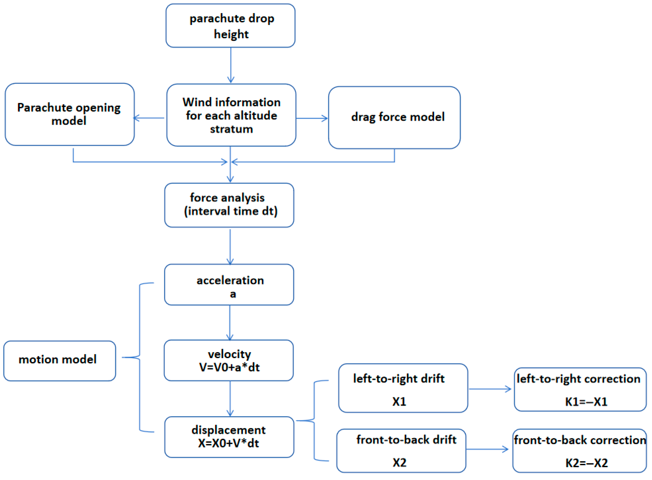
Through an extensive review of the literature and an engineering case study, this work summarizes a typical method model of linear airdrop prediction commonly used in current practice, and its flow is shown in Figure 1:
In the calculation process of the flow chart, the height of the airdrop is clarified first, and then based on the experimental and implementation experience data, the table is checked to obtain the falling time t of the corresponding object parachute system and the before-and-after correction benchmark value X. Before the implementation of the airdrop, the wind field of each airdrop height and the following height layers is detected by the lidar working in Doppler Beam Sharpening (DBS) mode. In the model, the height layer refers to dividing the vertical height of the airdrop area into several continuous intervals. The thickness of each interval is called the stratification interval, which is used to refine the modeling of the vertical distribution of the wind field. Take the example of setting up a height layer at 100 m intervals, and the wind field distribution expression is shown in Equations (1).
W ( H ) = [ v ( H ) , d ( H ) ]
In Equation (1) W(H) is the wind field vector of height H where H∈[(0,100) … (100n − 100,100n)] n ∈ Z+, v(H) is the wind speed of height H in m/s, d(H) is the wind direction of height H in degrees, and n is the number of height layers. Z+ represents the set of positive integers, used to constrain the value of n in the height layer division. After obtaining the wind speed of each height layer below the air drop height, the wind field vectors of each height layer are synthesized to obtain the synthetic wind speed, and the synthesis algorithm is shown in the following equation:
W ¯ = [ V , D ]
V = ( ( s u m x ) 2 + ( s u m y ) 2 ) 1 / 2 / n
D = a tan 2 ( s u m x , s u m y )
In Equation (2), W ¯ is synthetic wind vector, V is the synthetic wind speed, and D is the synthetic wind direction. In Equation (3), s u m y = i = 1 n v ( 100 n ) sin ( d ( 100 n ) ) represents the vector accumulation of wind speed components in the y-direction of each altitude layer, and the components are calculated by the sine value of wind speed v and wind direction d; s u m y = i = 1 n v ( 100 n ) cos ( d ( 100 n ) ) represents the vector accumulation of wind speed components in the x-direction of each altitude layer, and the components are calculated by the sine value of wind speed v and wind direction d.
After the synthetic wind vector is obtained, the vector is decomposed in the direction of the airdrop aircraft navigation to obtain V1, and in the vertical direction of the airdrop aircraft navigation to obtain V2. At this time, in the linear model of the airdrop parachute system, the parachute system produces an offset speed close to the wind speed along the wind direction. According to the expression of the displacement, you can obtain the airdrop’s amount of before-and-after correction K1, and the left-and-right corrections K2. They are calculated respectively as shown in the following equation:
K 1 K 2 = X + V 1 t V 2 t

2.2. Analysis of Methodological Models

This method is based on the assumption that the wind field has a linear effect on the airdrop process, and the validity of its motion model needs to satisfy the following prerequisite assumptions:
(1) The airdrop parachute at all altitudes has uniform and equal descent velocities;
(2) The wind speed of the airdrop process is approximately equal to the motion speed of the airdrop after being affected by the wind.
As noted in the research of Tang et al. (2016) [27], assumption (1) is questionable because the airdrop process involves multiple distinct stages: cargo platform extraction, main parachute straightening, parachute inflation, stable descent, and landing buffering. Each stage exhibits unique motion characteristics, making the assumption of uniform descent velocity unrealistic.
In assumption (2), the object parachute system is regarded as a weak inertial system. In fact, in the scenarios of actual application of airdrop, the mass of the load object can range from several hundred kilograms to several tons [28], which belongs to the strong inertial object. This assumption will lead to a large computational error in the case of large changes in wind speed at various altitudes.
Suppose the mass of the object is m, the horizontal wind speed is Vwind, and the deflection speed of the object is Vobj. The force Fwind exerted by the air on the object is as follows:
F w i n d = 1 2 ρ a V w i n d 2 C d A
In the formula, C d is the drag coefficient, ρ is the air density at the altitude where the parachute system is located, and A is the projected area of the parachute. At this time, the acceleration of the object due to inertia is a h = ρ a V w i n d 2 C d A / 2 m . This acceleration drives the object’s velocity to gradually approach the wind speed from 0 and form a first-order inertial response: d V o b j / d t = ρ a C d A ( V w i n d V o b j ) / 2 m . Letting the initial condition Vobj (0) = 0, we can obtain V o b j ( t ) = V w i n d ( 1 e ρ a C d A t / 2 m ) . Then, we can define the inertial time constant as τ = 2 m / ρ a C d A . When t = τ , Vobj = Vwind(1 − e−1) ≈ 0.63 Vwind; when t = 3 τ , Vobj = Vwind(1 − e−1) ≈ 0.95 Vwind. It can be seen that when the mass m is larger, the inertial time constant τ is greater, and the response of the inertial system is slower simultaneously. In the linear model, it is assumed that VobjVwind, which is equivalent to neglecting the inertial term and assuming that τ 0 or m ≈ 0. But in reality, m > 0, τ > 0, so Vobj < Vwind, and the displacement error is
Δ x e r r o r = 0 t t o t a l ( V w i n d V o b j ( t ) ) d t = V w i n d t t o t a l · τ t t o t a l ( 1 1 e t t o t a l / τ t t o t a l / τ )
When ttotal << τ , Δ x e r r o r 1 / 2 V w i n d t t o t a l · t t o t a l τ . It can be seen that it is proportional to the mass.
When the load mass is large like m = 1000 kg and the projected area A = 50 m2, τ 81.7 s , the ttotal < τ , Vobj < 0.63 Vwind. Therefore, we can consider that the weak inertia assumption holds only when m → 0. The difference between the deflection velocity and the wind speed increases significantly with the increase in mass; thus, the linear model will inevitably overestimate the displacement.
Based on the comprehensive analysis above, the existing airdrop prediction model has a gap with the actual situation under the reasonable consideration of the impact of wind speed. And it fails to completely describe the airdrop process from the objective physical law, which is prone to cause a large computational error. To overcome this limitation, it is necessary to construct a more accurate prediction model from the perspective of multi-physical-field coupling. Therefore, this work proposes an MPDE model that integrates radar detection of wind fields, aerodynamic characteristics of parachutes, and parachute deployment processes. Through multi-scale parameter coupling analysis and dynamic equation solving, this model achieves precise characterization of the motion trajectory of airdrop targets.

3. Multidimensional Parameter Dynamic Evolution Prediction Method

After the above analysis, the linear air drop prediction model cannot well describe the objective air drop process. Its performance is limited by the validity of its methodological premise, and there is a large possibility of uncertainty and error. Therefore, this work proposes an MPDE airdrop prediction model based on multi-model analysis, and its algorithm flow is shown in Figure 2:
The MPDE airdrop prediction model shown in the flow chart of Figure 2 is an algorithmic model designed to comprehensively consider physical phenomena and interactions at different scales, enabling accurate airdrop object motion analysis and guidance strategies. At different scales, the macro-scale includes the wind direction and speed in the atmospheric environment; the mesoscale includes the shape, size, and material of the object parachute system; and the microscale includes the aerodynamic characteristics and drag coefficient of the object parachute system affected by the fluid among other micro-level parameters. The inputs at multiple scales are coupled with each other to affect the output of the motion model. In the model, the macro-scale wind field determines the overall trend of the parachute’s movement. The meso-scale structural characteristics influence its force pattern in the wind field and interact with the macro-environment. Micro-scale aerodynamic parameters (such as air density and changes in drag area) finely adjust the trajectory through physical models like Newton’s second law. These three scales are coupled via dynamic equations, collectively acting on the output of the motion model to achieve comprehensive prediction of the airdrop target’s trajectory.
In the algorithm, after specifying the height of the airdrop, based on the same wind field information as the linear model, the system is analyzed in the wind field by establishing the opening model and the traction model of the object parachute system. The motion state is analyzed by Newton’s second law, and the Runge–Kutta method is applied to analyze the equation of motion to obtain the offset landing point of the airdrop and to compute the correction of the offset guidance.

3.1. DBS Radar Wind Field Inversion Method

The DBS radar wind field inversion method is a technique that utilizes the Doppler velocity data of lidar or wind profiling radars to invert the atmospheric wind field. Its core principle is to infer the three-dimensional wind field by analyzing the radial velocities detected by the radar beam at different azimuths and elevation angles, and by combining the radar geometric model with the dynamic constraints of atmospheric motion.
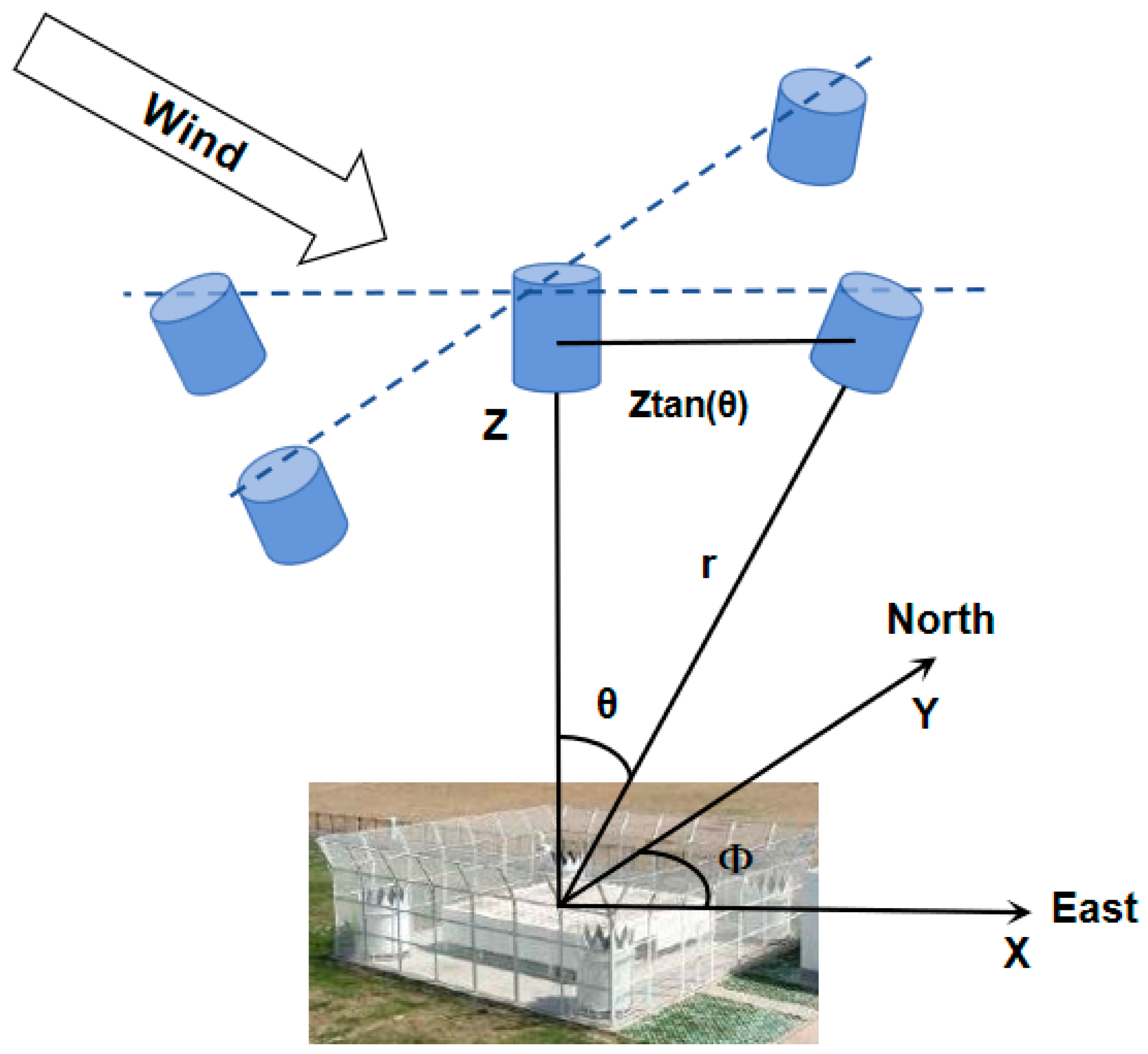
Commonly used DBS modes include the five-beam and three-beam modes. Taking the five-beam DBS algorithm as an example, its principle is shown in Figure 3:
In Figure 3, r is the radial distance from the target to the radar and θ is the angle between the inclined beam and the vertical direction. Φ represents the azimuth angle of the inclined beam projection on the horizontal plane relative to the north direction. When the radar operates in the DBS mode, it emits high-frequency electromagnetic waves and receives the backscattered signals from scatterers such as aerosols and precipitation particles in the atmosphere. According to the Doppler effect, the radial velocity Vr can be expressed as
V r = λ f d 4 π R
where f d is the Doppler frequency shift, λ is the wavelength, and R is the distance between the radar and the target. When the radar detects the wind field using the five-beam DBS method, it emits radar waves in the vertical direction and in four directions around the vertical direction at a specific angle. Typically, this angle ranges between 10° and 30°, and there is also a certain angular interval between each of the inclined beams. The radial velocity Vz measured by the radar’s vertical beam represents the wind speed in the vertical direction.
In the horizontal direction, assume that the horizontal wind speed is Vh, the direction iss α, and the angle between the projection of the inclined beam on the horizontal plane and the north direction is φ i (i = 1, 2, 3, 4). According to the geometric relationship, the radial velocity Vi of the inclined beam can be expressed as
V i = V h cos ( α φ i ) sin ( θ ) + V z cos ( θ ) ( i = 1 , 2 , 3 , 4 )
For the four inclined beams, four equations of the above form can be obtained. By combining these equations and using mathematical methods such as the least squares method for solving, the horizontal wind speed and wind direction can be derived.

3.2. Analysis of Drag Force Model of Object Parachute System

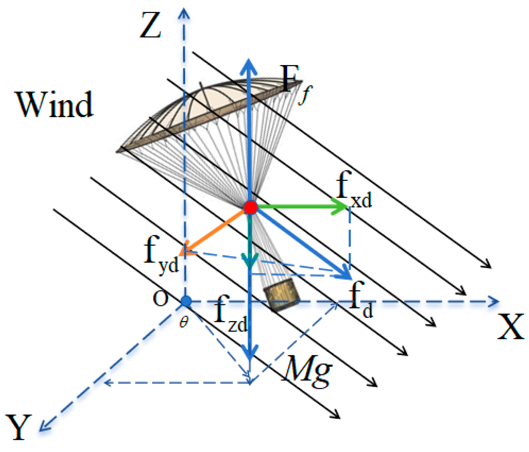
In this work, the parachute and its load are mainly subjected to gravity M g , air resistance F f , and the drag force f d generated by the relative motion of wind in the air.
The drag force f d is decomposed orthogonally in the X, Y, and Z directions. The force in the X direction is f x d , the force in the Y direction is f y d , the force in the Z direction is f z d , and g is the gravitational acceleration at the current latitude. Its force analysis is shown in Figure 4.
Figure 4 illustrates the core force relationships of the parachute system during the airdrop process. Through the labeling of coordinate systems and force vectors, it intuitively presents the orthogonal decomposition of gravitational force, wind-induced drag force, and air resistance.
Air can be considered as a Newtonian fluid and the expression for the traction force on the parachute system is
f d = π D 2 C d ρ a δ V δ V 8
In Equation (10), δ V = V w V b .
The size of the C d value of the object parachute system can be set to a reference value of 0.4 when calculating [29]; D is the equivalent windward diameter of the object parachute system, V w is the background ground-to-ground wind speed, and V b is the velocity of object parachute system’s motion to the ground.
The expression of atmospheric density variation with height [30,31] derived from Boltzmann’s energy distribution law is as follows:
ρ a = N r 0 ( r 0 r ) 4 e G M ¯ m kT ( 1 r 1 r 0 )
In Equation (11), m = μ / N A .
N r 0 is the number density of molecules on the surface of the Earth, N r 0 ≈ 19.52 × 1024 m−3, the average radius of the Earth r0 ≈ 6.371 × 10⁶ m, r is the distance from the center of the Earth to the position of the object parachute system, the universal gravitational constant G = 6.67 × 10⁻¹¹ m3kg−1s−2, the Earth’s mass M ¯ ≈ 5.975 × 1024 kg, Boltzmann constant k = 1.3806 × 10⁻²³ J/K, T is the thermodynamic temperature, T is taken as the temperature drop of 273.7K for every 100 m of rise, N A is Avogadro’s constant, N A = 6.0220 × 10²³ mol−1, and μ is the molar mass of the gas.

3.3. Parachute Opening Model Analysis

The research of the parachute opening model involves several aspects, including the dynamic analysis of the opening process [32], fluid–solid coupling simulation [33], and optimization of the opening efficiency [34].
The purpose of this work is to study the effect of wind field on the parachute system airdrop through hydrodynamic analysis to calculate the motion of the parachute system in the wind field. Combined with the above force analysis, this work focuses on the variation in parachute opening area projection during airdrop. In the analysis of the force inflation process for large parachutes, the commonly used formula for drag area variation derived by Knacke [35] through extensive experimental data analysis is adopted. Guo et al. (2012) [36] used Hermite curve to calculate the resistance area of parachute clothing in the overfilling stage, which can be approximated by fitting the change in open parachute projected area with time into the form of a quadratic curve. Its expression is given as follows:
A = A d + ( A f A d ) ( t t d t f t d )
In the formula, Ad and Af represent the projected area of the parachute canopy at the undeployed initial moment and the steady state, respectively; td and tf correspond to the initial deployment time and the final inflation time of the parachute canopy.

3.4. Parachute System Motion Modeling Analysis

According to the force analysis of the parachute system above and combined with Newton’s second law, the a x , a y , and a z of gravitational acceleration under the force in the X, Y, and Z directions are calculated as follows:
a x = π D 2 C d ρ a δ V x δ V x 8 M
a y = π D 2 C d ρ a δ V y δ V y 8 M
a z = π D 2 C d ρ a δ V z δ V z / 8 M g M
where δ V x , δ V y , and δ V z are the resultant velocity of wind speed and parachute speed in the X, Y, and Z directions, respectively. Assuming that the initial speeds of the object parachute system in the X, Y, and Z directions after leaving the cabin are V x 0 , V y 0 , and V z 0 , the displacements in the three directions can be obtained by integrating the accelerations in the three directions in the time domain. Assuming that the initial position of the object parachute system under the Cartesian coordinate system is (X0, Y0, Z0) and the initial time is T = 0, the coordinates of the predicted position of the object parachute system at the moment T = T0 are shown in Equation (16):
( X 0 + 0 T 0 ( V x 0 + 0 t a x ( τ ) d τ ) d t , Y 0 + 0 T 0 V y 0 + 0 t a y ( τ ) d τ ) d t , Z 0 + 0 T 0 V z 0 + 0 t a z ( τ ) d τ ) d t )

3.5. Runge–Kutta Method

Civil airdrops typically range from 300 to 1500 m, while military operations may reach several thousand meters. Parachute diameters span from 1 m (for small UAV payloads) to 30 m (for large equipment), and cargo weights range from 50 kg [7] to 5000 kg [19].
In analyzing the motion process of the MPDE airdrop prediction model, this work adopts the Runge–Kutta method [37] for the calculation of the motion process, and takes the fourth-order Runge–Kutta method (RK4) as an example of its basic principle as follows:
Assume that the differential equation and the initial conditions are as in Equation (17):
d y d x = f ( x , y )
In Equation (17), y ( x 0 ) = x 0 .
Its iterative formula is
y n + 1 = y n + ( 1 / 6 ) ( P 1 + 2 P 2 + 2 P 3 + P 4 )
P 1 = h f ( x n , y n )
P 2 = h f ( x n + h / 2 , y n + P 1 / 2 )
P 3 = h f ( x n + h / 2 , y n + P 2 / 2 )
P 4 = h f ( x n + h , y n + P 3 )
During the airdrop process, the object moves at high speed, and both field experiments and simulations must align with the computational conditions of the real hardware environment. The first-order Runge–Kutta method (Euler method) features low computational complexity (O(N)), which highly matches the real-time requirements of embedded systems. This ensures that simulation results directly reflect actual deployment scenarios. Therefore, we adopt the first-order Runge–Kutta method (Euler method) for approximate calculations to meet real-time computing needs. At this time, the iterative expression is
y n + 1 = y n + h f ( x n , y n )
t n + 1 = t n + h
The simulation of its computational process is shown in Figure 5.
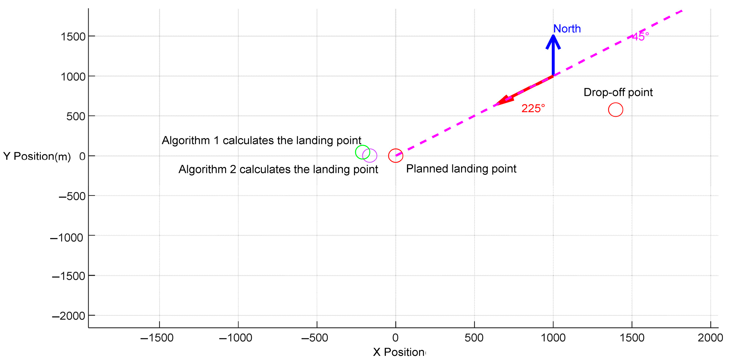
Figure 5 shows the calculation of the airdrop process based on the Runge–Kutta method without considering wind field detection error. The simulation focuses on the integration of wind field layers and motion equations, in which an altitude layer is set every 100 m and the wind field model of each altitude layer is randomly generated according to the normal distribution. The arrow vectors of each altitude layer (at 100 m intervals) in the figure represent the x and y components of the horizontal wind field input in the simulation under the Cartesian coordinate system. The length of the vectors is proportional to the wind speed, and the direction corresponds to the actual wind direction. The parameters used in the simulations, including airdrop altitude, parachute size, and cargo weight, are all derived from the field experiments described in Section 5. The parameter values fall within the general airdrop parameter ranges mentioned above. Figure 5a shows the trajectory in the side view of the sailing direction, Figure 5b shows the trajectory in the side view of the vertical sailing direction, and Figure 5c shows the 3D spatial trajectory of the airdrop. To visualize the method’s trajectory calculation logic, a schematic top-view of drop points under idealized conditions is shown in Figure 6. This illustration does not include experimental validation data.
The dotted line in the figure is the drop-off path, which is at an angle of 225° with the north. The drop-off point marked by a red circle represents the position where the airdropped object exits the cabin. The planned landing point, and the landing points calculated by two algorithms are marked with circles where Algorithm 1 is marked with a green circle and Algorithm 2 is marked with a purple circle. The accuracy of the algorithms can be evaluated by comparing the relative positions of the planned landing point and the landing points calculated by the algorithms.

4. The Impact of Model Input Errors on Airdrop Prediction Methods

The linear airdrop prediction method in this work is primarily related to the input of the wind field model; the multidimensional parameter prediction method is associated with wind field information, parachute deployment status, force analysis model, and other related physical models. Both airdrop prediction methods involve the input of wind field information, which in actual airdrop processes can be affected by equipment performance, accuracy of inversion algorithms, human operational errors, and other factors.
To analyze the stability of the two methods, this work investigates the impact of wind field detection errors on the models of the two methods via the RGA (Relative Gain Array) theory, aiming to analyze the influence mechanism and verify the simulation results through numerical methods. The field experiments in Section 5 obtained wind field data of the altitude layers passed by the airdropped objects during the airdrop implementation through lidar scanning (see Table 1 below). This dataset will be used as a typical scenario input to support the simulation analysis of the impact of wind field errors in this section, so as to explore the robustness of the model under actual wind field conditions.

4.1. RGA Theory

RGA theory is a general method used to analyze the interaction among control variables in a multivariable control system. It helps designers to optimize the control strategy and improve the stability and performance of the system by quantitatively analyzing the interactions among control variables [38].
In this section, the wind field detection error at each altitude layer is introduced as an input. Subsequently, the effects of the two airdrop model inputs on the drop point output are analyzed, and ultimately, the effect of the wind field detection error on the model performance is analyzed through the RGA theory.

4.1.1. RGA Analysis of Linear Model

In the linear airdrop prediction model, the input variable is the wind speed detection error { Δ V i } at each altitude layer, the output is the drift of the aircraft in the heading direction Xk, and the drift in the vertical heading direction is Yk. At this point, the transfer function matrix G is
G = X Δ V 1 X Δ V 2 X Δ V n Y Δ V 1 Y Δ V 2 Y Δ V n
In Equation (25),
X Δ V i = ( 1 n j = 1 n ( V j + Δ V j ) cos ( θ ) T ) Δ V i = T cos ( θ ) n
Y Δ V i = ( 1 n j = 1 n ( V j + Δ V j ) sin ( θ ) T ) Δ V i = T sin ( θ ) n
n is the height stratum; θ is the angle between wind direction and heading. At this point, the transfer function matrix is
G s i m = T ( cos ( θ ) ) n T ( cos ( θ ) ) n T ( sin ( θ ) ) n T ( sin ( θ ) ) n
Calculate the relative gain matrix RGA:
R G A s i m = G s i m G s i m 1 = 1 0 0 1

4.1.2. RGA Analysis of Multidimensional Parameter Air Drop Prediction

In the multidimensional parameter model, the input is the wind speed detection errors { Δ V i } at each altitude layer, and the outputs are the displacement errors of the airdropped object in the horizontal ground direction Xp and the vertical ground direction Yp. Unlike the linear model, this model couples wind field forces, parachute aerodynamic forces, and inertial forces through Newton’s second law. Its transfer matrix Gsim simultaneously reflects the dynamic interactions of wind speed components, parachute motion velocities, and aerodynamic parameters including drag coefficient Cd, air density ρ , and equivalent diameter D.
The expressions of the transfer function matrices Gdrag and Gsim are the same. At this point, the transfer matrix in the horizontal direction is
X p Δ V i x = 0 T   0 t a x Δ V i x d τ d t
Y p Δ V i y = 0 T   0 t a y Δ V i y d τ d t
In Equations (30) and (31),
a x Δ V i x = 1 2 C d ρ a D ( 2 ( V i x v x ) ( V i x v x ) Δ V i x )
a y Δ V i y = 1 m ( 1 2 C d ρ a D ( 2 ( V i y v y ) ( V i y v y ) Δ V i y ) )
where Vix and Viy are the horizontal and vertical components of the wind speed in the ground-based coordinate system for the i-th altitude layer, respectively; Vx and Vy denote the horizontal and vertical components of the parachute velocity in the ground-based coordinate system, respectively, and Viy = 0 in general.
Gsim,11 represents the influence of horizontal wind speed errors on downrange displacement, and the terms C d ρ D 2 / 8 m in its expression reflect the amplification effect of parachute aerodynamic forces on wind speed. Gsim,21 = Y p / V i x reflects the indirect effect of horizontal wind speed errors on crossrange displacement, which is caused by the vector synthesis of wind field and parachute motion. Similarly, Gsim,12 and Gsim,22 characterize the influence of vertical wind speed errors, but in actual scenarios, Viy ≈ 0, so the horizontal components are mainly concerned.
At this point, the multidimensional parameter drop prediction model relative gain matrix is:
R G A d r a g = G d r a g G d r a g 1 = 1 0 0 1

4.1.3. Conclusion of the RGA Analysis

The diagonal elements of the relative gain matrices for the two models concerning wind speed detection errors are all 1. This indicates that wind field errors affect the outputs of the two models independently. Based on this finding, we further analyze the specific forms and elements of the transfer functions to uncover the error propagation mechanisms of the two models.
The transfer matrix of the multidimensional parameter airdrop prediction model considers more complex dynamics. This is evident from the expressions of the two transfer function elements. The linear model’s error distribution exhibits sinusoidal and cosine characteristics ( X k cos θ , Y k sin θ ), which directly stem from its core assumption that the parachute’s horizontal velocity equals the wind speed. Consequently, displacement errors are determined uniquely by the projection of the wind vector onto the heading coordinate system, representing pure kinematic superposition. A wind direction detection error shifts the error phase by Δθ, as the synthetic wind angle becomes θ + Δθ, leading to deviations like X k = T · V ¯ cos ( θ + Δ θ ) , instead of X k = T · V ¯ cos θ .
The sensitivity of the multidimensional parameter prediction method to wind speed detection errors increases with the increase in parachute area, air density, and other parameters.
To compare the sensitivities of the two models to wind speed detection errors, we analyze how such errors affect the prediction accuracy of the landing point in the aircraft’s navigation direction. Specifically, we divide the element of the transfer matrix for the multi-dimensional parameter airdrop prediction model by the corresponding element of the linear model’s transfer matrix, resulting in
R G X = n C d ρ a D ( V i x V x ) T 2 cos ( θ )
In Equation (35), the value of RGX represents the ratio of non-robustness between the MPDE model and linear model under wind field error. A larger RGX value indicates that the robustness of the MPDE model is lower than that of the linear model. It means that compared with the condition of no wind field detection error, when there is a wind field detection error, the prediction accuracy of the MPDE model will deteriorate faster and decrease more.
The expression shows that the value of RGX increases with the increase in the number of height layers n and the landing time T. It is also positively correlated with the velocity difference between the wind speed and the airdropped object. In the actual rescue airdrop process, the height of each altitude layer is generally set according to the radar resolution, usually ranging from 75 to 150 m, and the airdrop altitude (600 m, 1000 m). Therefore, n  (6,13); meanwhile, Cd > 0.4 [29], ρ a = 1.225 kg/m3.
Through calculation, when the mass of the airdropped object exceeds 2 kg, to ensure that the landing velocity V of the object is less than 5 m/s, the diameter D of the parachute must be greater than 1 m. According to statistical data based on long-term experience in a certain field of airdrop operations, the estimated airdrop landing time T  (57 s, 75 s), the initial horizontal velocity of the airdrop Vx0 (100 m/s,200 m/s), and the wind velocity Vix of each altitude layer at the airdrop altitude is much less than Vx0.
By comprehensively analyzing the above situations and making estimations, in scenarios such as airdrop rescues, the airdrop aircraft has a high cruising speed with a large airdrop payload. In general, the resolution of wind radar ranges from 75 m to 150 m. From historical mission records, the payload mass ranges from 2 tons to 5 tons. This requires a large parachute area which ranges from 10 m2 to 30 m2, and at this time RGX >> 1. That is to say, the multi-dimensional parameter airdrop prediction model is more significantly affected by the wind speed detection error in such airdrop activities, and because the numerator of the RGX expression contains the term (VixVx), this influence becomes even more pronounced in environments where the wind speed varies greatly across different altitude layers.

4.2. Error Analysis Simulation Verification

In the process of wind field detection, the error generally comes from the systematic error brought by the performance of the equipment and the random error caused by human operation. In order to verify the conclusion of the above analysis, this work introduces the systematic error and random error on the basis of the measured wind field data to analyze the impact of wind field detection error on the airdrop results.
To ensure the authenticity of the wind field data, the simulated wind fields are derived from the lidar-measured data in Table 1 collected during two days of airdrop experiments.

4.2.1. Validation of Wind Field Error Impact Mechanism

Through the RGA theory, the sensitivity of the MPDE model to the wind field observation error is positively correlated with the parachute area; the airdrop error of the linear model is a trigonometric function with the wind field error, and the phase will also change with the wind field error.
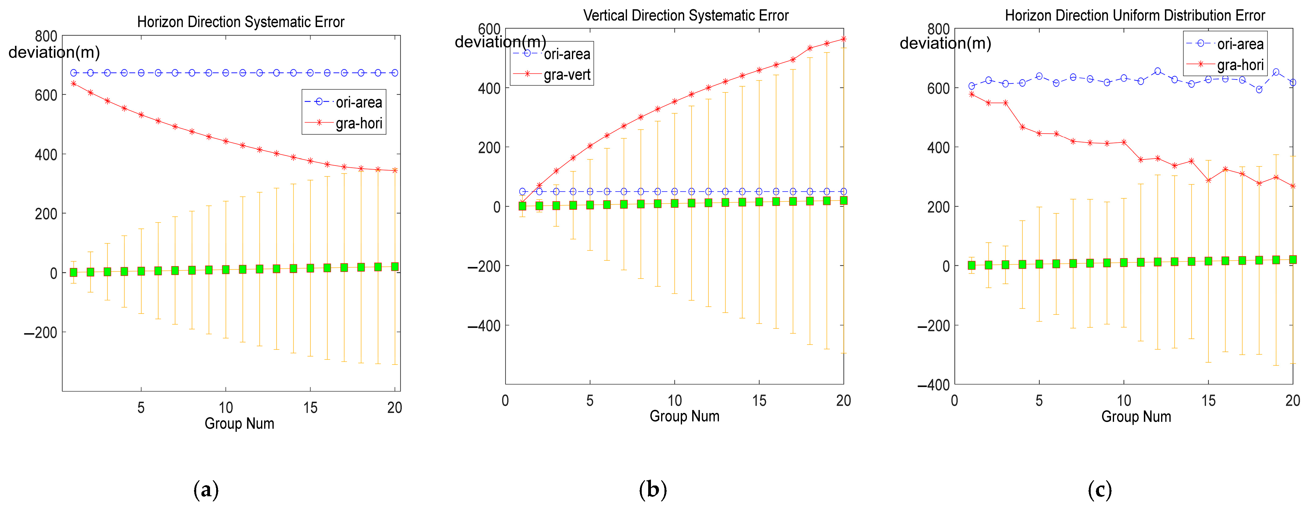
In order to verify the relationship between the parachute area in the MPDE model and prediction error under the wind field observation error, according to the experimental results of Zhao et al. (2020) [39] and distribution of data in Table 1, the systematic error is analyzed by setting the fixed wind speed detection error at each altitude layer to be 2 m/s. The random error is analyzed by introducing a uniform distribution error with a range of ±2, a normal distribution error with a mean of 0 and a variance of 2 for verification.
In the simulation process, the high-wind-shear experimental wind field data mainly come from Day 2 of the field experiment (see Table 1 above for data details, where Day 2 corresponds to the second experimental day). The growth gradient of the parachute projected area in the horizontal direction is set to be 5 m2 and the projected area in the vertical direction is set to be 100 m2 on the basis of the initial projected area. The results of the simulation under the various types of wind-field detection errors are shown in Figure 7:
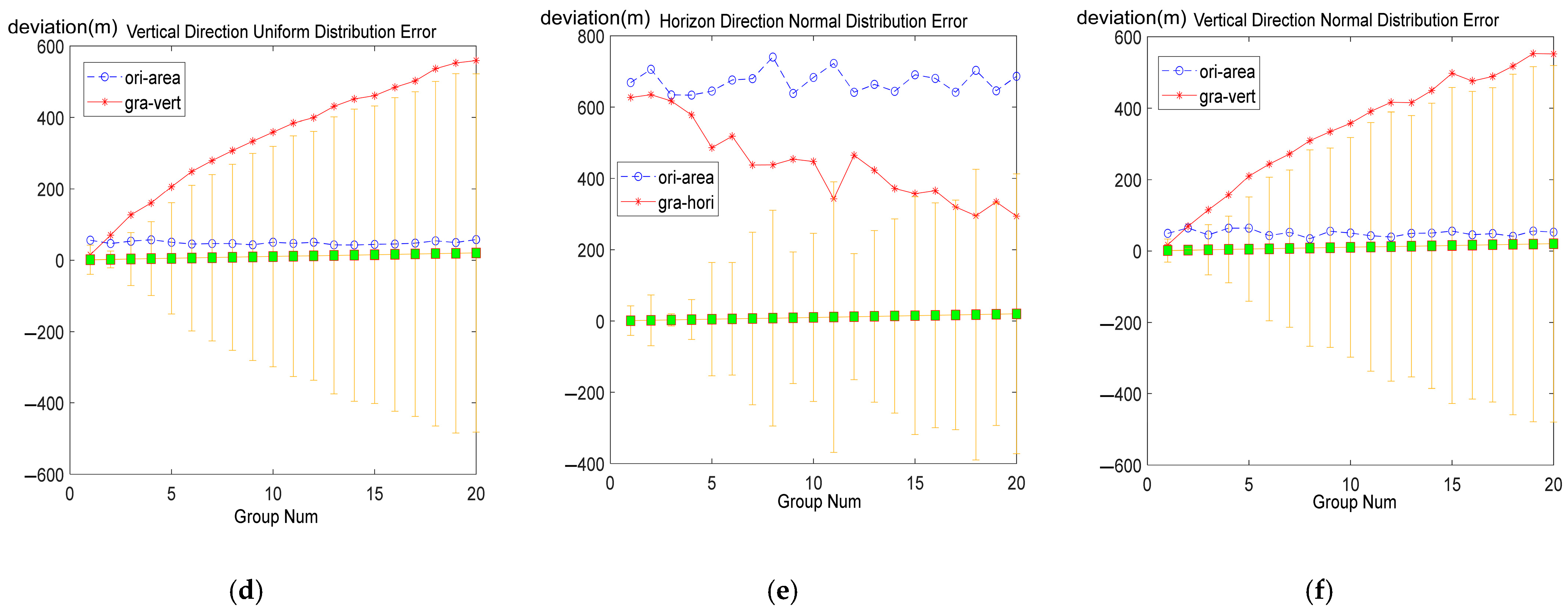
In Figure 7, the solid line represents the variation in airdrop error magnitude after gradient increment of the corresponding parachute area, and the dashed line partly indicates the change in the airdrop error under the original area; the length of the error bar on the horizontal axis represents the difference between the airdrop error caused by the change in area and the airdrop error of the original area. Because the focus is on the trend of the airdrop error caused by the change in the area, in order to facilitate the presentation, the dashed line and the solid line longitudinal coordinates are equivalently shifted when the plotting is performed from the original data.
From Figure 7a,b, it can be seen that under the wind detection error caused by the equipment performance, the airdrop error increases with the increase in area.
Focusing on even groups in Figure 7a, the error bar intervals were extracted to calculate the half-width. Let the half-width of the error interval be Y and the number of groups be X. Fitting the variation in the error bar with the number of groups according to a linear relationship yielded the equation Y = 26.1X + 15.7. This indicates that with each increment of 1 group in the horizontal projection area, the error dispersion increases by an average of 26.1 m, which demonstrates the “amplification effect” of area increase on error fluctuations. In the analysis, we introduce the coefficient of determination R2 [40], which is used to measure “the proportion of variation in true values explained by model predictions”. The value ranges between 0 and 1, where a value closer to 1 indicates that the model has a stronger ability to explain the data and a better fitting effect. After calculation, the data of Figure 7a shows R2 = 0.99, indicating a strong positive correlation between the error mean and the discretization degree, which verifies the law of “the larger the error, the wider the fluctuation range”. Similarly, in Figure 7b, the variation relationship equation of the error bar with the number of groups is Y = 35.2X − 49.8, with R2 = 0.99, which also demonstrates the universality of the law of “the larger the error, the wider the fluctuation range”.
Figure 7c,d represent the effect of parachute area on the airdrop error under the uniform detection error, which also characterizes the effect of the radar equipment error on the detection of the data. According to Figure 7c,d, it can be seen that the parachute area and the airdrop error under this type of error also show a clear positive correlation. Figure 7e,f show the effect of parachute area on airdrop error under normal error, which is used to simulate the error distribution caused by personnel operation in the process of detecting the wind field, and it can be seen from the figure that as the parachute area increases, the overall airdrop error is also increasing.
Calculations show that for the data in Figure 7c–f, the coefficient of determination R2 > 0.99, and the slopes of the linear equations describing the relationship between error bars and the number of groups in each figure are all greater than 0. Therefore, it can be assumed that in the MPDE model, under the influence of the wind field detection error, the parachute area is positively correlated with the airdrop error.
To verify the effect of the synthetic wind direction in the linear model on the performance of the airdrop under the wind field detection error, the following simulations are performed:
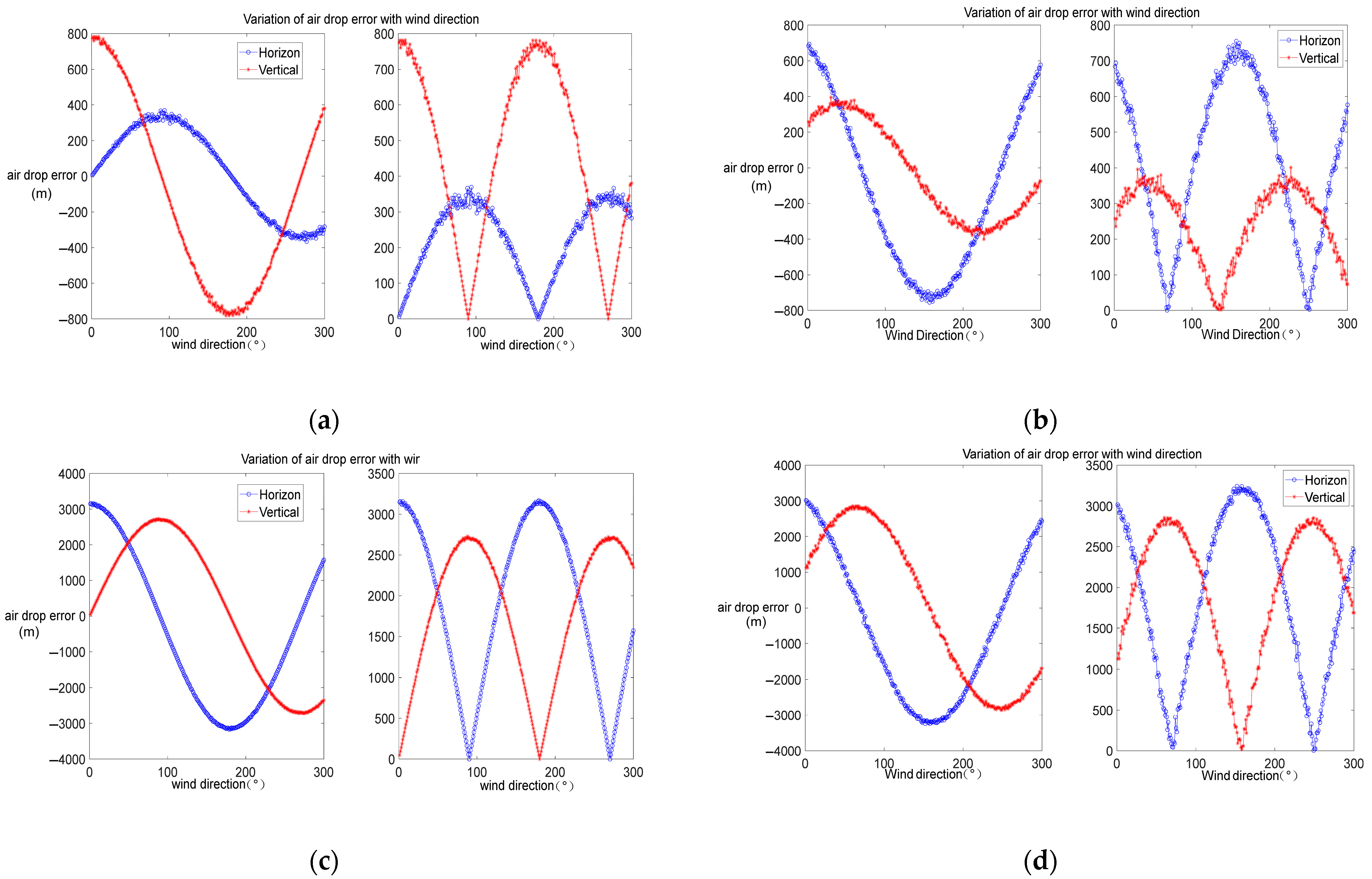
Assuming the airdrop course is due north at a flight path height of 700 m, wind speeds are set according to the daily wind speeds of each altitude layer. The wind direction of each layer is identical, changing sequentially from 0° to 300° at a 1° gradient referencing due north, with uniform distributions of wind speed and direction errors applied to each layer. The computational simulation results are shown in Figure 8.
The left subplots of Figure 8a–d show the relationship between the airdrop error and the actual wind direction under different wind speeds and wind directions, and the right subplot shows the absolute value of the airdrop error. The blue dots in the figure represent the air drop error in the horizontal direction, and the red dots represent the air drop error in the vertical direction.
In the linear airdrop model, the error shows a trigonometric relationship with the angle between the synthetic wind direction and the heading, where the error expression can be written as E cos θ , E sin θ . When the wind direction detection error follows a uniform distribution Δ θ ~ U ( a , b ) , its mean value is μ = ( a + b ) / 2 , making the actual synthetic wind direction become Δ θ + θ . Consequently, the error function transforms into E sin ( θ + Δ θ ) or E cos ( θ + Δ θ ) .
From a probabilistic perspective, the expected value of the error can be calculated via integration: E [ E ] = 1 / ( b a ) a b sin ( θ + Δ θ ) d ( Δ θ ) = ( cos ( θ + a ) cos ( θ + b ) ) / ( b a ) .
By simplifying using trigonometric sum-to-product formulas, when the interval [a,b] is symmetric about the mean μ , the integration result is equivalent to sin ( θ + μ ) , indicating that the phase shift of the error distribution exactly equals the mean value μ .
Taking Figure 8b as an example, the wind speed error is maintained at 0.3–0.8 m/s, while the wind direction error follows a uniform distribution of 15–25° with a mean value of 20°. Compared with Figure 8a (where the wind direction error is 0°), the sinusoidal curve in Figure 8b is overall shifted leftward by approximately 20°. From a phase perspective, this indicates a significant change in the phase of the error distribution. The 20° phase shift in Figure 8b is completely consistent with the mean value of the wind direction error, which well verifies the theoretical derivation. When the mean value of the wind direction error is positive, the curve shifts leftward; conversely, if the mean value of the wind direction error is negative, the curve will shift rightward. In Figure 8d, under the conditions of wind speed errors of 5–5.5 m/s and wind direction errors of 15–25°, the phase shift of the error distribution curve still follows the above rules. Even with the superposition of high wind speed errors, the characteristic that the mean value of wind direction errors determines the phase shift amount remains significant. Due to the influence of wind speed errors, the amplitude of the error curve also increases significantly. This indicates that in complex wind field error environments, the dominant role of wind direction errors on the phase of error distribution remains unchanged, but the superposition of wind speed errors makes the overall error characteristics more complex. It can be seen that the airdrop error with the actual wind direction shows a more obvious delta function relationship, and its function phase changes with the size of the wind field error. At the same time, the larger the wind field error is, the larger the magnitude of its airdrop error is.

4.2.2. Simulation Validation of Model Performance Under Wind Field Detection Error

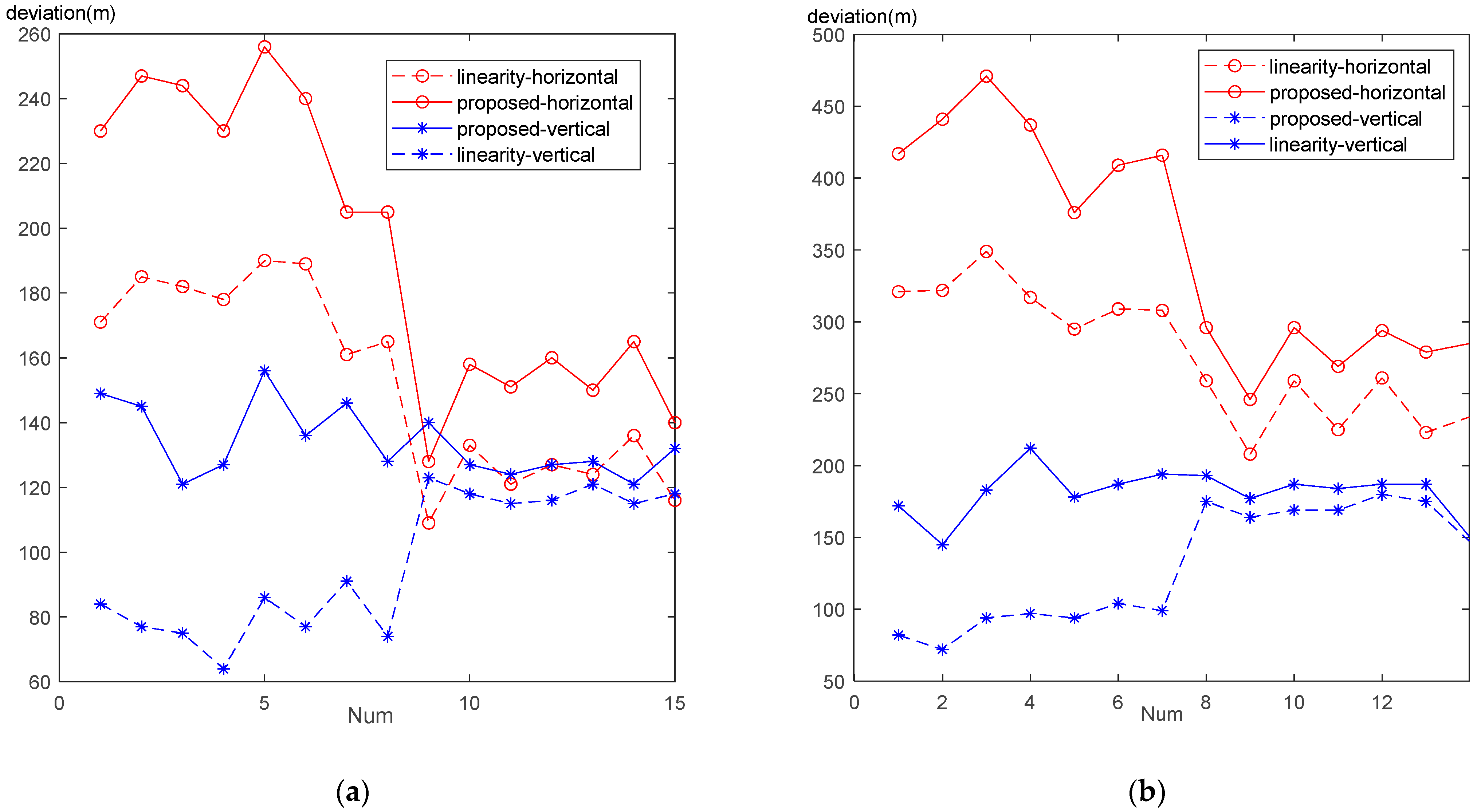
From the above analysis, this study concludes that in actual airdrop rescue scenarios, the linear model exhibits better stability than the MPDE model under wind field measurement errors. To verify the conclusion of this analysis, this work incorporates random wind detection errors following a normal distribution based on the measured wind field data, in accordance with airdrop parameters such as the payload mass, parachute area, and aircraft cruising speed from field experiments. Then, the airdrop prediction deviations are calculated according to the two algorithm models, and a comparative analysis is conducted. According to the experimental results of Zhao et al. (2020) [39], in this work, 20–30% of the wind speed amplitude is set as the moderate wind field detection error level, which can cover the conventional fluctuations in low wind speeds and the equipment precision errors in non-precipitation periods. Additionally, 30–50% of the wind speed amplitude is set as the high error level to reflect the larger errors that may occur in extreme weather conditions or high-altitude detection. The computational simulation results are shown in Figure 9.
Figure 9a,b show the drift error increase of front–back and left–right of the airdrops. The drift errors are calculated by the linear model and the proposed MPDE model for the random detection error amplitude of the wind field at 20–30% and 30–50% of the detected wind speed. Respectively, the dashed line represents the linear model, the solid line represents the proposed MPDE model, the circle point lines represent the front–back errors, and the star-shaped lines represent the left–right errors. In the two figures, the error results under the wind field data of airdrop day1 are shown before the group number 1–7, and the error results under the wind field data of airdrop day2 are shown in the group number 8–15. From the data, it can be seen that the airdrop error increase calculated by the linear model under the same wind field detection error is generally smaller than that of the MPDE model, and the simulation results are in line with the theoretical analysis above. Therefore, it can be considered that the linear airdrop model has better robustness under the wind field detection error.

5. Method Model Performance Validation

In this study, based on measured meteorological data and the results of field airdrop experiments, the performance gain of the optimized method is quantitatively analyzed by comparing the deviation between the predicted results of the two methods and the actual results.

5.1. Experimental Procedure

This field experiment lasted for two airdrop days. In total, 5 batches of experiments, amounting to 12 sets, were conducted over these two days. One batch is defined as one takeoff and landing of the airdrop aircraft, during which all identical cargo carried in the cabin is airdropped. Each aircraft sortie carries 1 to 3 sets of cargo, totaling 12 sets. Moreover, in each batch, multiple sets of identical cargo were successively airdropped using parachutes of the same model. The process of a single day’s airdrop is as follows:
Before airdrop deployment, lidar was used to detect the wind field at the deployment point multiple times in a five-beam DBS scanning mode. Scanning was performed in five directions: east, west, south, north, and vertical, with a pitch angle of 30°. The last detected wind field before the drop was used as the reference wind field due to the short interval between the drop batches.
The airdrop altitude was 600 m for all batches on Day 1 and 700 m for all batches on Day 2. The airspeed range of the airdrop aircraft was (200 m/s,400 m/s). The mass of the airdropped objects was over 1000 kg.
The airplane flies at heading 225°, and after the cargoes are out of the cabin, the airplane speed Vh, the moment t and the height H of the cargoes out of the cabin in each batch, the moment tK and the height Hk of the parachute opening, the stable falling speed Vk after the parachute is fully opened, and the airdrop landing point data are recorded. The distribution of wind field information is shown in Table 1, where the wind direction is the meteorological wind direction.
Table 1 records the wind speed and wind direction data at different altitude layers below the airdrop altitude on two experimental days (Day 1 and Day 2). The wind information of Table 1 covers the altitude of the airdrop height, with each layer at intervals of 100 m. On the first experimental day (Day 1), the wind speed was concentrated at 4.2–8.7 m/s (below the 600 m layer), the wind direction was 281–299° (northwest wind), and the wind field showed high stability. On the second experimental day (Day 2), the wind speed fluctuated significantly. The wind direction gradually changed from 193° at the 700 m layer to 129° at the layers below 300 m, indicating obvious wind shear.
After obtaining the meteorological data, two algorithmic models are used to calculate the drop point of the airdrop based on the initial information such as the location and speed of the airdrop. The calculation process based on the linear model is shown in Figure 1. The descent times of such parachute can be obtained by looking up the corresponding table. In the MPDE model calculation, due to experimental conditions, we cannot know the open state of the object parachute system. That is, the projected area of the open parachute in the sailing direction and the vertical direction cannot be known. Considering the consistency of the object parachute system and the cargo for each day of the airdrop, the experimental treatment is as follows:
Firstly, based on the wind measurement data and the first set of airdrop data of the first batch of the day, the parachute parameters are obtained by algorithmic fitting of the actual drop point. These parameters mainly include the projected area of the parachute in the heading direction and vertical direction of the airdrop aircraft Sx, Sy, Sz. Then the prediction deviation is calculated based on the obtained parachute parameters, which are brought into the later batches of the various groups of parachute landing data. During the calculation process, the acceleration of gravity g = 9.81, air density ρ = 1.225, parachute drag coefficient Cd = 1.2, and the performance of the model are obtained by comparing the predicted drop point positions of the two models with the actual drop point positions.

5.2. Analysis of Experimental Results

This experiment utilizes a circular parachute. Considering that the projected area of the circular parachute is fitted as a quadratic relationship with time variation, and there is also a quadratic relationship between the area and diameter, in this work, the time variation and the projected diameter of the circular parachute are approximated as a linear relationship in the calculations using the MPDE model.
The experiment was conducted over two days, with six groups of experiments performed each day. After each group of experiments, we calculated the landing point straight-line distance prediction error (E1) and left–right distance prediction error (E3) of the linear airdrop prediction algorithm, the straight-line distance prediction error (E2) and left–right distance prediction error (E4) of the MPDE algorithm. The landing point straight-line distance precision improvement rate of the MPDE algorithm was computed as (E1E2)/E1, and the left–right distance precision improvement rate was computed as E3/E4. The straight-line distance and left–right distance precision improvement rate was shown in Table 2.
In Table 2, “Day 1” and “Day 2” represent the six groups on the first and second days of the experiment. “Straight-line Improvement” represents the landing point straight-line distance prediction distance precision improvement rate of the MPDE algorithm (computed as (E1E2)/E1), and “Left–right Improvement” represents the landing point left–right distance prediction distance precision improvement rate (computed as E3/E4). As shown in Table 2, the MPDE algorithm generally improves the precision of the predicted airdrop landing points compared with the linear prediction algorithm.
Statistically, the MPDE target prediction method airdrop drop point slant distance prediction accuracy is improved by 52.03% on average, and the drop point left–right distance prediction accuracy can be improved by one order of magnitude. In the optimization algorithm, there is also a relative increase in the individual errors of the later batches. This is analyzed as being caused by the changes in the actual wind speed compared to the last wind measurement, leading to computational errors.
From a comprehensive point of view, by establishing an MPDE airdrop prediction model to optimize the airdrop prediction algorithm, its airdrop prediction performance can be greatly improved.
Although the experiments only covered data from two days, the wind field characteristics on Day 1 and Day 2 already encompass stable and high wind shear scenarios. Moreover, maintaining a 70.97% precision improvement rate under the high wind shear scenario on Day 2 demonstrates the model’s robustness in extreme conditions. The statistical results of 12 experiments show that the accuracy of the MPDE algorithm has an average improvement of 52.03%. Combined with theoretical extrapolation, this fully validates the effectiveness of the method in typical airdrop scenarios.
Specifically, the preceding analysis has shown that in scenarios involving wind field detection errors, the linear airdrop model exhibits higher robustness due to its simple parameterization. Nevertheless, in real-world airdrop scenarios with inherent wind field detection errors, the MPDE model still demonstrates better prediction accuracy. This advantage is attributed to the MPDE model’s precise characterization of airdrop system dynamics through partial differential equations, enabling it to have higher fidelity in modeling complex physical processes. Therefore, for scenarios with strict requirements on landing accuracy, such as precise delivery by civil unmanned aerial vehicles and aerospace payload recovery, the MPDE model can provide more reliable predictions and is more suitable for such scenarios requiring physical fidelity. Meanwhile, this study on the impact of wind field detection errors on the performance of the two types of airdrop models can also provide a quantitative basis and decision-making reference for the rational selection and application of airdrop prediction models under different environmental conditions.

6. Conclusions

In order to improve the accuracy of airdrops in complex environments, this work first identifies the existing linear airdrop prediction methods and analyzes the inadequacies of these methods. Then, under the framework of fluid mechanics analysis, it establishes a drag force model, a parachute deployment model, and a motion model for airdrop targets in wind fields. Finally, by fusing key parameters across multiple dimensions from these models, it develops an MPDE airdrop prediction model.
The performance of linear and MPDE models is analyzed through field experiments. The experimental results show that the optimized MPDE model can improve accuracy by 52.03% compared with the linear model, and the accuracy of offset calculation in the vertical heading direction can be improved by one order of magnitude. Meanwhile, in order to verify the robustness of the two models under the input error, this work analyzes the generation mechanism of the prediction error of the two methods under the wind field detection error through the RGA theory. The simulation results show that the linear model is less sensitive to wind field detection errors and demonstrates stronger robustness compared to the MPDE model. Its airdrop error exhibits a trigonometric function relationship with the angle between the resultant wind direction and the heading, and the phase of the function shifts according to the error. The error sensitivity of the MPDE model is positively correlated with both the parachute area and air density.
In summary, for the airdrop linear prediction model, the systematic error of wind detection can be fully recognized in the actual application process, and the corresponding heading can be selected to reduce the impact of the wind detection error by combining with the demand. For the MPDE model, the physical model of the parachute system’s opening process can be further explored in subsequent research to optimize the force analysis. Meanwhile, considering the MPDE airdrop prediction model’s sensitivity to wind detection errors, investigating a more accurate wind speed inversion algorithm can enhance the overall performance of the airdrop prediction algorithm. This study also has certain limitations. For instance, the model for the movement of air-dropped objects did not adequately account for the non-Newtonian behavior of air under complex flow conditions. Additionally, the accuracy of simulating turbulent effects during the interaction between air-dropped objects and wind fields still needs improvement. The dynamic adjustment mechanisms for some parameters also require further optimization. Future research will focus on advanced turbulence simulation techniques, such as large eddy simulation (LES) and direct numerical simulation (DNS), to optimize the prediction models for the movement trajectories of air-dropped objects. Machine learning algorithms can be introduced to mine the nonlinear correlations among multi-dimensional parameters including wind speed, parachute area, payload mass, and airdrop errors, aiming to establish adaptive correction models for different scenarios. The demand for high-spatiotemporal-resolution wind field detection can also be combined with radar polarization technology [41]. Through the collaborative processing of polarization channels, the ability of radar to analyze atmospheric aerosol scattering signals can be enhanced. The time modulation method can be used to improve the dynamic response speed of wind field detection, thus providing more accurate layered wind field data for the MPDE model.
Meanwhile, the particle swarm optimization algorithm can be used to optimize the decomposition process of the wind field polarization scattering matrix [42], optimize the dynamic adaptation mechanism of multiple parameters in the wind field inversion model, reduce detection errors caused by temporal and spatial variations of the wind field, and provide more accurate input parameters for the MPDE model.
Wind tunnel simulation experiments and field airdrop tests under extreme weather conditions can be carried out to calibrate model parameters and verify the robustness of the multi-dimensional parameter dynamic evolution method.

Author Contributions

Conceptualization, X.W. and J.Y.; methodology, X.W.; software, X.W.; validation, X.W., J.Y. and J.L.; formal analysis, Y.L.; investigation, X.W.; resources, Y.L.; data curation, X.W.; writing—original draft preparation, X.W.; writing—review and editing, J.Y. and J.L.; visualization, X.W.; supervision, J.Y.; project administration, J.Y.; funding acquisition, Y.L. All authors have read and agreed to the published version of the manuscript.

Funding

This research received no external funding.

Data Availability Statement

Due to the nature of this research, participants of this study did not agree for their data to be shared publicly, so supporting data are not available.

Acknowledgments

The authors would like to thank the support of the laboratory and university.

Conflicts of Interest

The authors declare no conflicts of interest.

References

  1. Wang, Y.; Yang, C.X.; Yang, H. Neural Network-based Simulation and Prediction of Precise Airdrop Trajectory Planning. Aerosp. Sci. Technol. 2022, 120, 107302. [Google Scholar] [CrossRef]
  2. Beijing University of Aeronautics and Astronautics. An Autonomous Homing Control Method for Precision Airdrop System Based on Model Predictive Control. Patent No.: CN202311177238.7, 20 October 2023. [Google Scholar]
  3. Nanfang College of Sun Yat-sen University. A Wireless Monitoring Node Delivery System for Environmental Events. Patent No.: CN202020471312.1, 8 January 2021. [Google Scholar]
  4. Cacan, M.R.; Costello, M.; Ward, M.; Scheuermann, E.; Shurtliff, M. Human-in-the-Loop Control of Guided Airdrop Systems. Aerospace Sci. Technol. 2019, 84, 1141–1149. [Google Scholar] [CrossRef]
  5. Li, G.; Cao, Y.; Wang, M. Modeling and Analysis of a Generic Internal Cargo Airdrop System for a Tandem Helicopter. Appl. Sci. 2021, 11, 5109. [Google Scholar] [CrossRef]
  6. Xu, R.; Chen, C.; Lu, S.; Li, Z. Autonomous Recovery from Spacecraft Plan Failures by Regulatory Repair While Retaining Operability. Aerospace 2022, 9, 40. [Google Scholar] [CrossRef]
  7. Zhang, F.; Wang, H.T. Precision Airdrop Systems in Europe and America. Ordnance Ind. Autom. 2007, 26, 7–8. [Google Scholar] [CrossRef]
  8. Sun, Q.L.; Yang, J.S.; Sun, H.; Chen, Z. A Review of Key Technologies for the Autonomous Homing of Parafoil Systems. J. Natl. Univ. Def. Technol. 2024, 46, 1–15. [Google Scholar]
  9. Long, J. Design of Precision Airdrop Control Device for UAV Based on STM32. Electron. Technol. Softw. Eng. 2019, 2, 83. [Google Scholar]
  10. Wang, S.N.; Chen, F. Research on Stable Control of Precise Bomb—Throwing for Individual—Soldier UAVs in Complex Terrain. J. Ordnance Equip. Eng. 2020, 41, 25–30. [Google Scholar]
  11. Liu, Z.C. Dynamic Modeling and Homing Research of Small Ram-Air Parachute; National University of Defense Technology: Hunan, China, 2013. [Google Scholar] [CrossRef]
  12. Cao, Y.; Nie, W.; Lian, X. Dynamic Modeling of a Transport Helicopter for Internal Cargo Airdrop. Int. J. Aerosp. Eng. 2024, 2024, 9183728. [Google Scholar] [CrossRef]
  13. Yang, M.S. Flight Dynamics Modeling and Simulation for Transport Airdrop. Master’s Thesis, Beijing University of Aeronautics and Astronautics, Beijing, China, 2010. [Google Scholar]
  14. Wang, Y.; Wang, G.; Sun, Y.; Gu, L.; Zhang, J. Airdrop dynamics modeling and simulation based on reduced multibody system transfer matrix method. Aerosp. Sci. Technol. 2025, 158, 109914. [Google Scholar] [CrossRef]
  15. Ward, M.; Cacan, M.; Scheuermann, E.; Costello, M. Use of Ground—Based Wind Measurements for Improved Guided Airdrop Accuracy; American Institute of Aeronautics and Astronautics (AIAA): Daytona Beach, FL, USA, 2015; pp. 845–862. [Google Scholar]
  16. Xu, X.; Qi, M.; Liu, S.; Sun, L. Research on the Airdrop Trajectory of Ram-Type Rapid Airdrop Airbag. Packag. Eng. 2015, 36, 35–38. [Google Scholar]
  17. Wang, Y.F.; Xue, Y.C.; Li, Q. Comparative Analysis of Wind Measurement by Balloon Trajectory Method and Wind Profiler Radar. Meteorol. Hydrol. Mar. Instrum. 2007, 3, 30–34. [Google Scholar] [CrossRef]
  18. Zhang, T.; Zhang, J.; Yang, J.; Meng, J. Comparison of Wind Field Data Measured by Satellite Scatterometers and Sea Surface Platforms. J. Mar. Sci. 2013, 31, 45–51. [Google Scholar]
  19. Yin, X.B.; Wang, Z.Z.; Liu, J.Y.; Jiang, J.S. A New Scheme for Eliminating the Remote Sensing Ambiguity of Co-/Counter-Wind Directions in Fully Polarimetric Microwave Radiometers—Algorithm Research. J. Remote Sens. 2009, 13, 42–48. [Google Scholar]
  20. Ma, Y.; Faizal, M.; Ishak, M.R.; Rahim, S.A.; Mustapha, M. Structural Fault Diagnosis of UAV Based on Convolutional Neural Network and Data Processing Technology. Nondestruct. Test. Eval. 2024, 39, 426–445. [Google Scholar] [CrossRef]
  21. Abari, C.F.; Chu, X.; Hardesty, R.M.; Mann, J. A Reconfigurable All-Fiber Polarization-Diversity Coherent Doppler Lidar: Principles and Numerical Simulations. Appl. Opt. 2015, 54, 8999–9009. [Google Scholar] [CrossRef] [PubMed]
  22. Hu, W.Z. Simulation on Flight Dynamics and Control of Parafoil Airdrop Systems; Nanjing University of Aeronautics and Astronautics: Nanjing, China, 2017. [Google Scholar]
  23. Wang, J.Z.; Chen, H.L. Research on Parachute Airdrop Based on Runge—Kutta Algorithm. Mod. Electron. Technol. 2010, 33, 124–126, 130. [Google Scholar]
  24. Ma, M.; Yang, R.; Rao, W.; Huang, Z. Research on the Optimization of the Starting Point Control for the Towed Airdrop Planning of Transport Aircraft. Comput. Simul. 2015, 32, 126–130. [Google Scholar]
  25. Li, W.; Huang, Z.; Zhou, Q.; Hao, H. Modeling and Simulation of Fixed—Point Delivery of Military Equipment under Complex Conditions. Ordnance Ind. Autom. 2011, 30, 41–44. [Google Scholar]
  26. Wei, L.; Zhang, D.; Zhang, R.; Zheng, S.; Lai, Y.; Fu, Y.; Hu, W.; Lv, Y. Research and Analysis on the Distribution Characteristics of the Atmospheric Wind Field in Jiuquan Area. Intensity Environ. 2023, 50, 57–63. [Google Scholar] [CrossRef]
  27. Tang, J.H. Simulation Calculation of the Dynamics of Vehicle—Mounted Gun Airdrop System; Nanjing University of Science and Technology: Nanjing, China, 2016. [Google Scholar] [CrossRef]
  28. Jing, Z.W.; Hou, Z.T.; Guo, Z.D. Flight Loads Design Technique for Flexible Aircraft Airdrop. Acta Aeronaut. Astronaut. Sin. 2014, 3511, 3037–3045. [Google Scholar]
  29. Incropera, F.P.; DeWitt, D.P. Fundamentals of Heat and Mass Transfer, 4th ed.; Wiley: Hoboken, NJ, USA, 1996. [Google Scholar]
  30. Da, D.A.; Yang, Y.T.; Tu, J.H. Research on the Characteristics of the Planetary and Interplanetary Atmospheric Environment in the Solar System. J. Astronaut. 2006, 27, 1306–1313. [Google Scholar] [CrossRef]
  31. Wang, G.; Tan, K.; Cao, C. Sedimentation Law and Drag Coefficient Model of Cuttings Particles with Different Shapes. Drill. Fluid Complet. Fluid 2022, 39, 707–713. [Google Scholar]
  32. Wang, C.L. Calculation Model and Analysis of Parachute Deployment Dynamic Load in Rocket Sled Test. J. Syst. Simul. 2018, 30, 4574–4579. [Google Scholar]
  33. Chen, C.; Guo, Q.L. A Numerical Model of Parachute Inflation and Deployment Based on the Arbitrary Lagrangian–Eulerian Method. Sci. Technol. Eng. 2021, 21, 801–807. [Google Scholar]
  34. Liu, X. Simulation Research on the Deployment Process of Parafoil Based on Fluid-Structure Interaction Method; Nanjing University of Aeronautics and Astronautics: Nanjing, China, 2019. [Google Scholar]
  35. Knacke, T.W. Parachute Recovery Systems Design Manual; Para Publishing: China Lake, CA, USA, 1992. [Google Scholar]
  36. Guo, P. Research on the Deployment Process of Large—Scale Parachutes; National University of Defense Technology: Changsha, China, 2012. [Google Scholar]
  37. Gao, X.G. Introduction to Aviation Military Aircraft; Northwestern Polytechnical University Press: Xi’an, China, 2002. [Google Scholar]
  38. Zhang, P.X.; Cao, Y.J.; Wang, H.F.; Cheng, S.J. Application of Relative Gain Array Method in Interaction Analysis of Multivariable Controllers for Flexible AC Transmission Systems. Proc. CSEE 2004, 24, 13–17. [Google Scholar] [CrossRef]
  39. Zhao, W.K.; Shan, Y.L.; Zhao, S.J. Research Progress of Low-Level Wind Shear Detection by Laser Radar. Meteorol. Hydrol. Mar. Instrum. 2020, 37, 97–100. [Google Scholar]
  40. Xueyan, X.; Buxi, L. Research on the Influence of Different Dependent Variable Selections on the Coefficient of Determination R2. J. Taiyuan Univ. Sci. Technol. 2007, 28, 3–8. [Google Scholar]
  41. Sui, R.; Wang, J.; Sun, G.; Xu, Z.; Feng, D. A Dual-Polarimetric High Range Resolution Profile Modulation Method Based on Time-Modulated APCM. IEEE Trans. Antennas Propag. 2025, 17, 1007–1017. [Google Scholar] [CrossRef]
  42. Wang, J.; Quan, S.; Xing, S.; Li, Y.; Wu, H.; Meng, W. PSO—Based fine polarimetric decomposition for ship scattering characterization. ISPRS J. Photogramm. Remote Sens. 2025, 220, 18–31. [Google Scholar] [CrossRef]
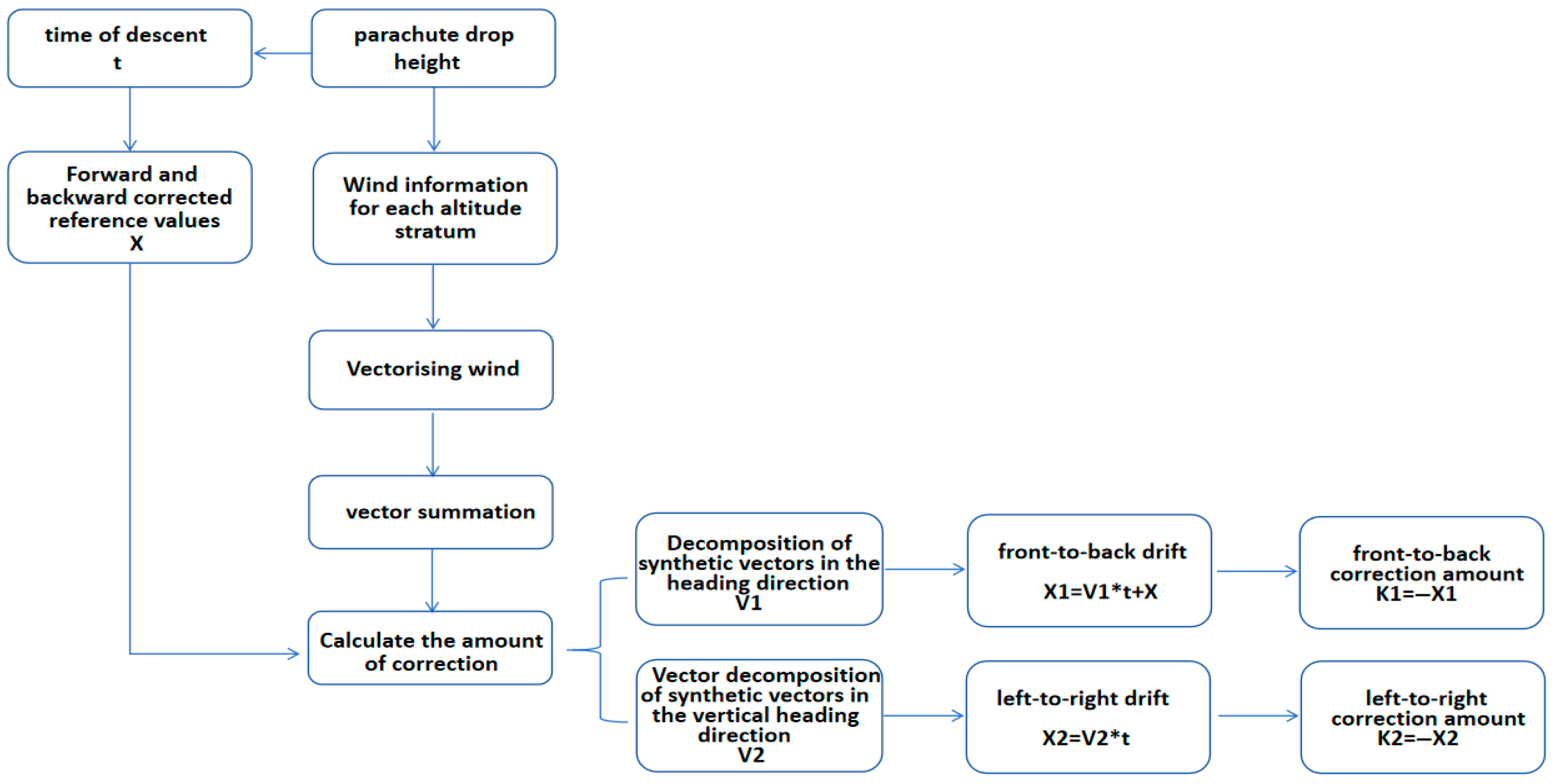
Figure 1. Typical method flow chart for linear airdrops.
Remotesensing 17 02476 g001
Figure 2. Flow chart of MPDE target prediction method.
Remotesensing 17 02476 g002
Figure 3. The principle of the five-beam DBS algorithm.
Remotesensing 17 02476 g003
Figure 4. Parachute system force analysis.
Remotesensing 17 02476 g004
Figure 5. Visualization of Euler method for motion equation solving. (a) X-direction airdrop process; (b) Y-direction airdrop process; (c) three-dimensional trajectory of the airdrop.
Remotesensing 17 02476 g005
Figure 6. Overhead view of airdrop site.
Remotesensing 17 02476 g006
Figure 7. Effect of parachute area on airdrop error under different wind field observation errors. (a) Effect of horizontal area on aerial drops under systematic detection errors; (b) effect of vertically oriented area on airdrops under systematic detection error; (c) effect of horizontal area on airdrops under uniformly distributed detection errors; (d) effect of vertical area on airdrops under uniformly distributed detection errors; (e) effect of horizontally oriented area on airdrops with normally distributed detection errors; (f) effect of vertically oriented area on airdrops under normally distributed detection errors.
Remotesensing 17 02476 g007aRemotesensing 17 02476 g007b
Figure 8. Relationship between wind direction and air drop error for different wind field errors. (a) Wind direction error = 0, wind speed error = 0.3–0.8/uniformly distributed; (b) wind direction error = 15–25, wind speed error = 0.3–0.8/uniformly distributed; (c) wind direction error = 0, wind speed error = 5–5.5/uniformly distributed; (d) wind direction error = 15–25, wind speed error = 5–5.5/uniformly distributed.
Remotesensing 17 02476 g008
Figure 9. Airdrop errors under two model wind speed errors. (a) Simulation of the 20–30% wind speed error; (b) simulation of the 30–50% wind speed error.
Remotesensing 17 02476 g009
Table 1. Meteorological wind records.
Height(m)1000900800700600500400300200100
DataDay1Wind speed (m/s)\\\\8.68.76.68.24.26
Wind direction (°)\\\\294295295297299281
Day2Wind speed (m/s)\\\2.52.61.610.215.110.76.2
Wind direction (°)\\\193139141133129129129
Table 2. Precision improvement of airdrop landing points per group under MPDE method.
Group123456
Day1
Straight-line
Improvement
87.84%8.50%75.39%49.41%48.07%11.02%
Day2
Straight-line
Improvement
88.11%75.14%45.54%56.62%66.68%70.97%
Day1
Left–right
Improvement
7.9289.0714.1252.1613.5830.028
Day2
Left–right
Improvement
7.932.8891.9632.2534.6925.571
Disclaimer/Publisher’s Note: The statements, opinions and data contained in all publications are solely those of the individual author(s) and contributor(s) and not of MDPI and/or the editor(s). MDPI and/or the editor(s) disclaim responsibility for any injury to people or property resulting from any ideas, methods, instructions or products referred to in the content.