Terrain and Atmosphere Classification Framework on Satellite Data Through Attentional Feature Fusion Network

Abstract

Surface, terrain, or even atmosphere analysis using images or their fragments is important due to the possibilities of further processing. In particular, attention is necessary for satellite and/or drone images. Analyzing image elements by classifying the given classes is important for obtaining information about space for autonomous systems, identifying landscape elements, or monitoring and maintaining the infrastructure and environment. Hence, in this paper, we propose a neural classifier architecture that analyzes different features by the parallel processing of information in the network and combines them with a feature fusion mechanism. The neural architecture model takes into account different types of features by extracting them by focusing on spatial, local patterns and multi-scale representation. In addition, the classifier is guided by an attention mechanism for focusing more on different channels, spatial information, and even feature pyramid mechanisms. Atrous convolutional operators were also used in such an architecture as better context feature extractors. The proposed classifier architecture is the main element of the modeled framework for satellite data analysis, which is based on the possibility of training depending on the client’s desire. The proposed methodology was evaluated on three publicly available classification datasets for remote sensing: satellite images, Visual Terrain Recognition, and USTC SmokeRS, where the proposed model achieved accuracy scores of 97.8%, 100.0%, and 92.4%, respectively. The obtained results indicate the effectiveness of the proposed attention mechanisms across different remote sensing challenges.

1. Introduction

The construction and modeling of new convolutional neural network (CNN) architectures is still an important domain of research and engineering work. One of the main motivations is to improve the performance of models in terms of architecture, where newer mechanisms and types of layers can be used. In recent years, attention modules have contributed to the reconstruction of many networks. These modules aim to enhance representation by emphasizing important spatial and channel-wise features during learning [1,2], but many proposed designs still lack attention to contextual adaptivity, especially in complex scenes.

Efficient training with limited data and minimal computational resources alongside performance is also a critical goal, especially in the context of remote sensing applications [3,4]. The larger the model, the more computing power will be needed to train it. This is due to the increase in the number of training parameters. It is also worth paying attention to the amount of training data and its size. Large data sizes will take longer to be processed by the network, but their reduction may contribute to the reduction in features and important properties describing the data. Considering these premises, new models are created and modified to find more accurate architectures than the known ones. However, recent methods often overlook the aspect of multi-scale features in image processing, which results in a model’s struggle with inter-class similarity in terrain recognition tasks [5,6].

Modeling new solutions also involves analyzing the information processed in the classifier itself. The construction of a CNN allows us to pay attention to feature extraction and its reduction using convolutional and pooling layers. In the final stage of processing, the results are flattened and transferred to dense layers that operate by classical neural networks. The output result is the probability of belonging to particular classes. To address existing gaps, hybrid models such as STNet and CTA-Net have introduced attention-based feature fusion to improve spatial–spectral integration [7,8]. Still, these approaches can be inattentive to context-aware interactions across fused features. Feature fusion in the context of neural classifiers is based on combining processing results from different layers. This allows for creating models that will not linearly analyze the image sample. An interesting aspect is the possibility of introducing many branches that will connect at some stage [9]. The use of the concept of feature fusion allows you to adapt the classifier to obtain a more accurate image representation, which should result in a faster and more accurate training process. Yet, many designs do not explicitly address the interference between fused features, leading to degraded interpretability or generalization.

The multi-branching nature of neural networks is based on the previously mentioned process of aggregating data from individual layers. Currently, there are many different methods, the most popular of which are concatenation by combining vectors or matrices, using sum or difference operations, or multiplication. In the case of the last one, i.e., multiplication, it is an operation performed on matrices. Still, multiplication is performed by multiplying elements in the same positions, which is called element-wise [10]. Average fusion can also be distinguished, either by using other statistical measures or by combining individual channels [11]. In remote sensing applications and especially with HSI image data, dual-branching allows the model to learn different aspects of feature representation. In [12] one branch focuses on locally present features, while the other one focuses on the global ones. By aggregating them later in the network, the model considered both the broader context of the processed data and the more detailed, regional context of the processed image.

In particular, the construction of such models is visible in the analysis of satellite images, which contribute to further processing. The ability to use satellites to perform graphical measurements on Earth results in large amounts of accurate data. An example of such an application is a system using multimodal artificial intelligence methods [13]. This research aimed to predict air quality by analyzing data contained in satellite images. Another solution is the [14] framework, which analyzes satellite data for flood index insurance analyses. An interesting approach was presented based on the analysis of global climate changes [15], which can be undertaken using satellite data. Recent advances, including transformer-based models like TGF-Net and DACN [3,16], showcase promising directions in remote sensing but still lack robust solutions for multi-resolution and experiments in remote sensing scenarios, where training data is limited.

Analysis of terrain is an important aspect in terms of understanding the surfaces. As a main application, drones and robots can be used. An example is the use of a CNN and time series [17]. The CNN in a temporal approach has been used, which involves recurrent neurons. Quite often, there is a need to create maps based on terrain data, which can also be performed using segmentation networks [18]. As part of the presented model, the authors showed a lidar scan that is transposed to a tensor and processed by 3D sparse convolution and convGRU layers. Learning transfer models are also used and modified for this task, like extending ResNet with a fully convolutional network [19]. It is also possible to combine the results of two terrain analysis results, an example of which is the hybridization of a CNN and support vector machines (SVMs) [20]. Not only are neural networks used for this classification problem but also PCA in combination with an SVM [21]. Feature fusion turned out to be an interesting alternative for creating new models, as evidenced by solutions like SSFCT and HyFusion, which combine CNNs and attention blocks for better spatial–spectral extraction [5,6]. As a result, the technique allowed for a much more complex idea of feature extraction and the ability to direct the classifier to important features. In recent years, researchers have noticed that feature fusion by combining two different convolutional networks to analyze hyperspectral images can be effective [22]. Additionally, in [23] the authors proposed a probabilistically optimized fusion model for better feature extraction, which significantly reduced information loss in the forward pass of the network. The presented merging allows for the fusion of features from both networks, where the authors point out that through this fusion, the network focuses on global features through superpixel analysis as well as on multi-scale local features. Another merger solution is the step-wise approach [24], which is based on a progressive localization decoder that adapts to the pyramid transformer. Again, in [25], the authors presented atrous convolutional operators with different dilation rates, which allow for feature fusion in detection networks of small objects in images. Multi-scale feature fusion combined with knowledge transfer can also increase the precision and accuracy of small object detection [26]. In the context of learning transfer, there are also other fusion methods such as adaptive fusion of feature maps using the feature pyramid network [27]. Fusion research has also shown that it is possible to create lightweight networks that use nested residual blocks [4]. This solution allows for obtaining an asymmetric structure of residual blocks. The proposed technique allows for more accurate image reconstruction than classical methods based on research results. There are also weighted feature fusion techniques in convolutional and weighting networks [28], which were dedicated to the problem of hyperspectral image classification. A promising approach was presented in [29], where the authors proposed an ensemble of transformer and convolution feature extractors for the task of satellite segmentation. However, the proposed solution struggled with flexible convolution on irregular segmentation masks, which needs to be studied and addressed further.

Based on the analysis of various solutions in the field of hyperspectral and satellite image analysis and various techniques, there is still a huge demand for more accurate artificial intelligence models. As part of the research, in this paper, we present a new framework for the analysis of satellite data in the context of terrain classification or the detection of some phenomenon. The framework is based on the storage and version control mechanism of the classifier in the cloud, to which users have access. The user can train the model on private data, but this will require additional verification. We propose a new convolutional neural network model for classification using feature fusion and attention mechanisms. The motivation for building such an architecture is to focus on the possibility of analyzing various features, which is necessary in the case of similar classes. The main contributions of this research are as follows:

• Presenting a framework for terrain classification based on satellite images, featuring novel ML methods and user-accessible model updates;
• Proposing a new dual-channel CNN-based backbone architecture is introduced, incorporating contextual attention and multi-head feature fusion to enhance semantic discrimination;
• Offering a lightweight and effective attention mechanism that dynamically re-weights feature maps based on spatial and channel-wise information;
• Conducting experimental analysis on public remote sensing datasets demonstrates that the proposed methods perform well and could be used in production.

2. Methodology

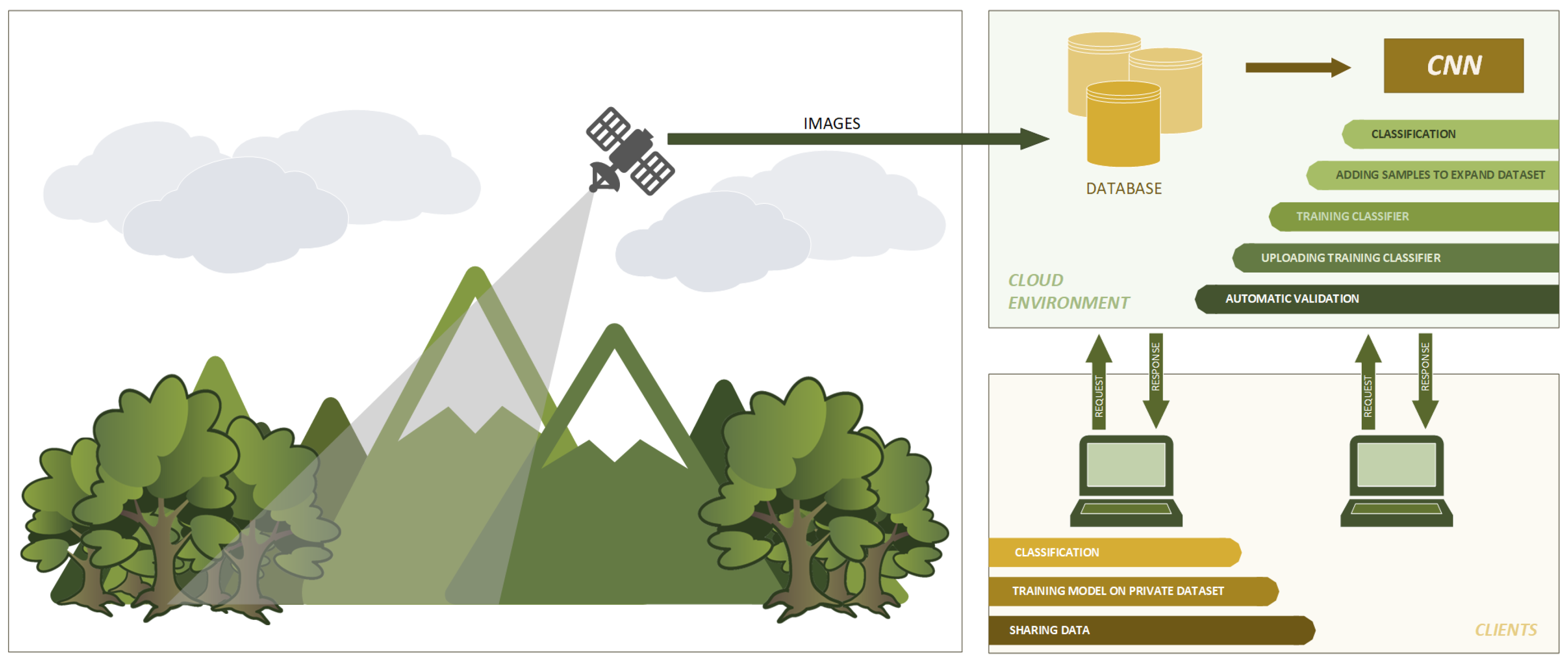
2.1. Framework Architecture for Terrain and Atmosphere Analysis Purposes

The possibility of performing satellite measurements means that we can analyze terrain or the atmosphere photographed from above. Practically, this enables quick analysis of the examined area in terms of its current condition. Moreover, comparing data over several minutes or even months is important for research or prediction purposes. Additionally, knowing the condition in a certain area can be used to react in the event of a certain event. One such example is a fire that contributes to the formation of a smoke cloud that should be distinguishable from the clouds present in satellite data. The analysis of this data is possible using artificial intelligence methods. Of course, intelligent solutions have some drawbacks, such as a long learning process or the problem of adapting the number of new classes to existing models. For this purpose, we propose a framework where satellite data can be saved in the cloud or on the local disk of the company or the user themselves. This data can be used to train a classifier or even perform a prediction operation.

Having the data stored in one of the two places mentioned above, we propose to place the classifier model itself in the cloud, which is publicly accessible. If data is sent directly to the cloud, the classifier can be trained locally using the data. The user can share their data to the cloud to increase the amount of data, but verification should be added to prevent the possible poisoning of the set (e.g., by incorrectly assigning labels). If the user does not want to share satellite data, he or she can perform the training process locally and share it in the cloud for others. This will also require verification to ensure the proper operation of the system in real time.

The data verification mechanism will be implemented by validating data and checking its correctness using the following formula:

$$\left\{\begin{array}{c}\mathrm{if}{y}_{true}==\lceil y_{p}red\rceil \mathrm{then}\mathrm{accept}\mathrm{sample},\hfill \\ \mathrm{in}\mathrm{other}\mathrm{case}\mathrm{reject}\mathrm{sample}.\hfill \end{array}\right.$$

(1)

In the case of a new model, verification is performed by determining accuracy values on local data. If the new model’s accuracy is higher than the current one, it is replaced. The idea of the operation is illustrated in Figure 1 and in pseudo-code form for the cloud in Algorithm 1.

Algorithm 1: Framework’s operation: cloud.

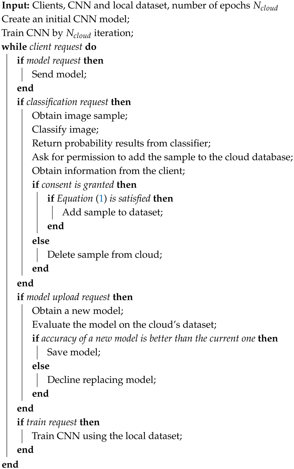
2.2. Proposed Neural Network Architecture

In this section, we present the construction of a CNN architecture based on various feature analyses and their fusion. For this purpose, three types of modules are presented successively and are ultimately used in the classifier. The model uses classic image processing layers such as convolution and pooling. The analyzed image is presented as a tensor I of dimensions $(w,h,d)$, where w is the width, h is the height, and d is the depth, initially depending on the color model.

A convolutional operation is denoted as ${\Lambda }_{n\times n}^{k,\mathrm{func}}(·)$, where $n\times n$ is the filter size, k is the number of filters, and func is the activation function. This operation extracts feature maps by applying the filter matrix (kernel) over the input tensor.

Along with convolution, pooling layers are used to reduce spatial dimensions by compressing features (e.g., with max or average operations). We denote max-pooling as ${{\rm Y}}_{n\times n}(·)$, where $n\times n$ is the window size of the pooling operation.

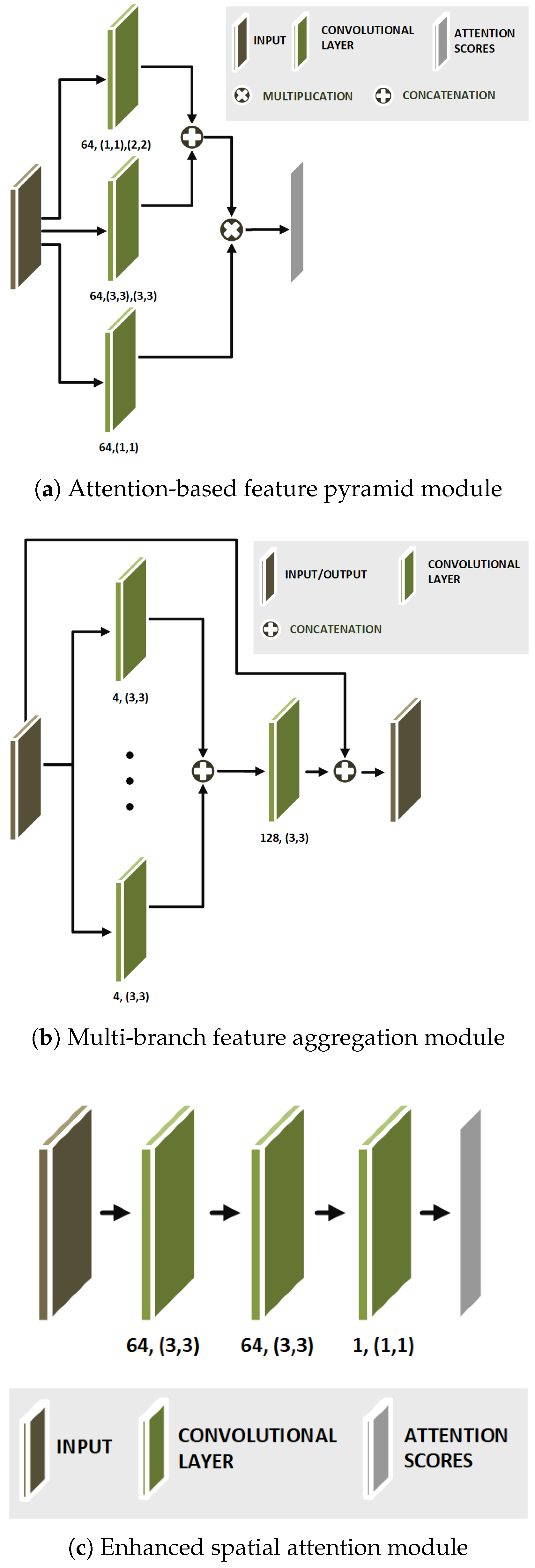
2.2.1. Enhanced Spatial Attention Module

The attention module focuses (see Figure 2c) on generating a matrix containing values in the range $\langle 0,1\rangle$, where each value indicates the importance of given values in this position. We apply three consecutive $3\times 3$ convolutions with 64 filters each to the input tensor x. The first two use ReLU activation to extract meaningful features, and the final uses a sigmoid function to produce attention scores in $[0,1]$. This ensures the output shape matches the input. The output of this attention module can be defined as follows:

$$y_{ESA}\left(x\right)={\Lambda }_{3\times 3}^{64,\mathrm{sigmoid}}\left({\Lambda }_{3\times 3}^{64,\mathrm{relu}}\left({\Lambda }_{3\times 3}^{64,\mathrm{relu}}\left(x\right)\right)\right),$$

(2)

where $y_{ESA}\left(x\right)$ is the attention score map.

The use of multiple convolution layers with a $3\times 3$ window allows for the extraction of global features. The resulting attention score matrix $y_{ESA}$ is then multiplied by the input tensor, which can be defined as

$$x^{\prime }=x·y_{ESA}.$$

(3)

2.2.2. Attention-Based Feature Pyramid Module

The next introduced mechanism is an attention-based feature pyramid (AFP) module (see Figure 2a). This module performs multi-scale analysis on the tensor x by applying atrous (dilated) convolutions and attention and then merging the results. The first operation performed on x is reducing the features of the input tensor x using a convolutional layer with 64 filters of size $1\times 1$. However, we propose to use an atrous convolutional layer (defined as ${\widehat{\Lambda }}_{n_1\times n_2,(d,d)}^{k,func}(·)$) instead of the classic one. This operator works by adding a dilatation rate parameter $(d,d)$, which introduces a larger distance between filters. The main advantage is the ability to analyze global features that take into account the context of the entire tensor. The whole attention process can be divided into consecutive steps.

The first operation reduces the features using

$$y_1\left(x\right)={\widehat{\Lambda }}_{1\times 1,(2,2)}^{64,\mathrm{relu}}\left(x\right),$$

(4)

where $\widehat{\Lambda }$ is atrous convolution with the dilation rate $(2,2)$.

The second operation applies

$$y_2\left(x\right)={\widehat{\Lambda }}_{3\times 3,(3,3)}^{64,\mathrm{relu}}\left(y_1\left(x\right)\right),$$

(5)

extracting larger-scale spatial features.

The attention enhancement uses

$$y_3\left(x\right)={\Lambda }_{1\times 1}^{64,\mathrm{sigmoid}}\left(x\right).$$

(6)

The final output is as follows:

$$y_{AFP}\left(x\right)=y_1\left(x\right)+y_2\left(x\right)·y_3\left(x\right).$$

(7)

2.2.3. Multi-Branch Feature Aggregation Module

The third block is multi-branch processing through convolutional layers and aggregation of features (see Figure 2b). We apply 32 parallel convolution operations, each with 4 filters of size $3\times 3$, followed by concatenation and ReLU activation:

$$y_4\left(x\right)={\Lambda }_{3\times 3,1}^{4,\mathrm{relu}}\left(x\right)\oplus {\Lambda }_{3\times 3,2}^{4,\mathrm{relu}}\left(x\right)\oplus \dots \oplus {\Lambda }_{3\times 3,32}^{4,\mathrm{relu}}\left(x\right),$$

(8)

where ⊕ denotes concatenation.

Next, we apply a $1\times 1$ convolution for dimensionality reduction and element-wise multiply the result with the original input:

$$y_{MBFA}\left(x\right)=x\otimes {\Lambda }_{1\times 1}^{64,\mathrm{relu}}\left(y_4\left(x\right)\right).$$

(9)

The introduction of the module allows for the extraction of features for tensors processed by a small number of layers but subjected to subsequent aggregation and reduction. As a consequence of these operations, local patterns and the hierarchy of features on individual tensor matrices can be detected.

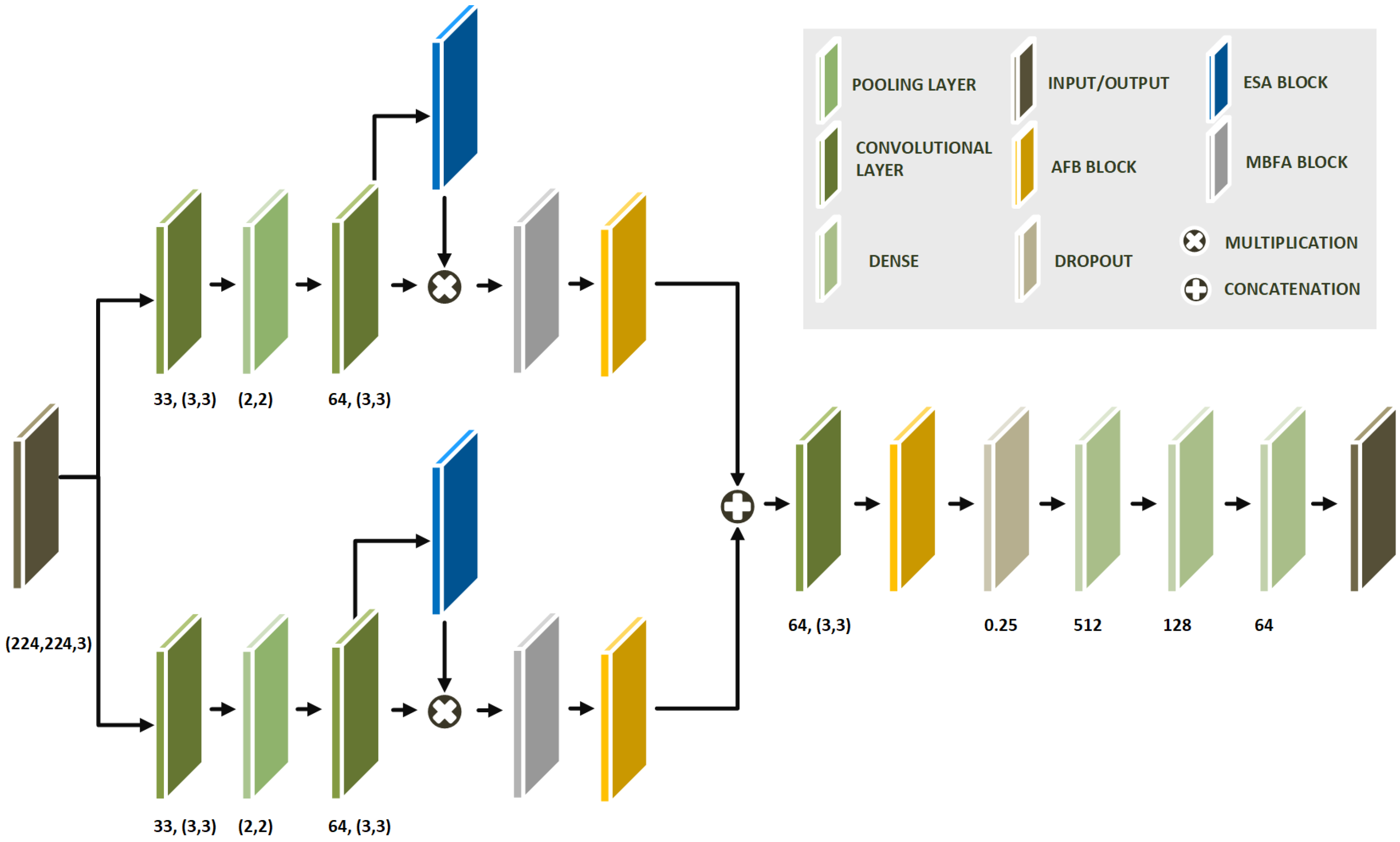
2.2.4. Model Architecture

We integrate the fore-described modules into a dual-branch CNN model for satellite image classification. The model starts by performing the convolution operation on the input, given as

$$x^{\prime }={\Lambda }_{3\times 3}^{32,\mathrm{relu}}\left(x\right).$$

(10)

Then, max pooling is performed to reduce the size of the image with a $2\times 2$ window, and another convolution is performed, which can be represented as

$$y_5\left(x^{\prime }\right)={\Lambda }_{3\times 3}^{32,\mathrm{relu}}\left({{\rm Y}}_{2\times 2}\left(x^{\prime }\right)\right).$$

(11)

Next, ESA is applied followed by MBFA and AFP modules:

$$Y_1\left(x^{\prime }\right)=y_{AFP}\left(y_{MBFA}\left(y_5\left(x^{\prime }\right)·y_{ESA}\left(y_5\left(x^{\prime }\right)\right)\right)\right).$$

(12)

In parallel, we introduce a second processing branch for the $x^{\prime }$ tensor, which is structured exactly the same. The output of the second branch can be presented as

$$Y_2\left(x^{\prime }\right)=y_{AFP}\left(y_{MBFA}\left(y_6\left(x^{\prime }\right)·y_{ESA}\left(y_6\left(x^{\prime }\right)\right)\right)\right),$$

(13)

where $y_6(·)$ is calculated the same way as in Equation (11). It should be noted that despite the same architecture, both branches initially have random filter values, which will be modified during training. Hence, the features extracted and processed by these branches can be unique and focus on different aspects of the input’s characteristics. In the next step, both branches are concatenated, followed by convolution and an AFP module. Following this, a dropout layer is proposed to stabilize the training process and prevent overfitting. This can be described as

$$Y_3\left(x^{\prime }\right)={\Gamma }_{0.25}\left(y_{AFP}\left({\Lambda }_{3\times 3}^{64,\mathrm{relu}}\left(Y_1\left(x^{\prime }\right)\oplus Y_2\left(x^{\prime }\right)\right)\right)\right).$$

(14)

The $Y_3$ value is flattened and passed to the next three dense layers composed of 512, 128, and 64 neurons with the ReLu function. The layer with 64 neurons is also equipped with an additional L1 and L2 regularization technique with parameters equal to 0.01. At the end, there is an output layer with the number of neurons equal to the number of classes and the softmax function. A visualization of the model is also presented in Figure 3.

The proposed loss function extends categorical cross-entropy with a term that penalizes overly confident predictions:

$$L(y,\widehat{y})=-\sum _{i=1}^N{y}_i·log\left({\widehat{y}}_i\right)+0.1·{\displaystyle \frac{1}{N}}\sum _{i=1}^N{\widehat{y}}_i,$$

(15)

where y is the one-hot label vector, and $\widehat{y}$ is the predicted probability vector.

3. Experiments

To evaluate the proposed model, three different datasets were used to analyze the performance of the proposal. The experimental descriptions and results obtained were divided into separate subsections. The obtained results are then summarized in a discussion in Section 3.4. For a quick overview, a brief description of each dataset as well as the obtained accuracy score is presented in

Table 1. Comparison between the datasets and the obtained accuracy scores in the experiments.

	Satellite Images	Visual Terrain Recognition	USTC SmokeRS
Description	Small-scale dataset focused on satellite-based land cover	Large-scale dataset for terrain classification with diverse surface textures	Medium-scale dataset for smoke and atmospheric condition recognition
Image Size	Varying	$64\times 64$	$256\times 256$
N. o. Classes	7	23	6
Train/Test Split	673/46	303,901/37,993	4980/1245
Accuracy [%]	97.8	100.0	92.4

.

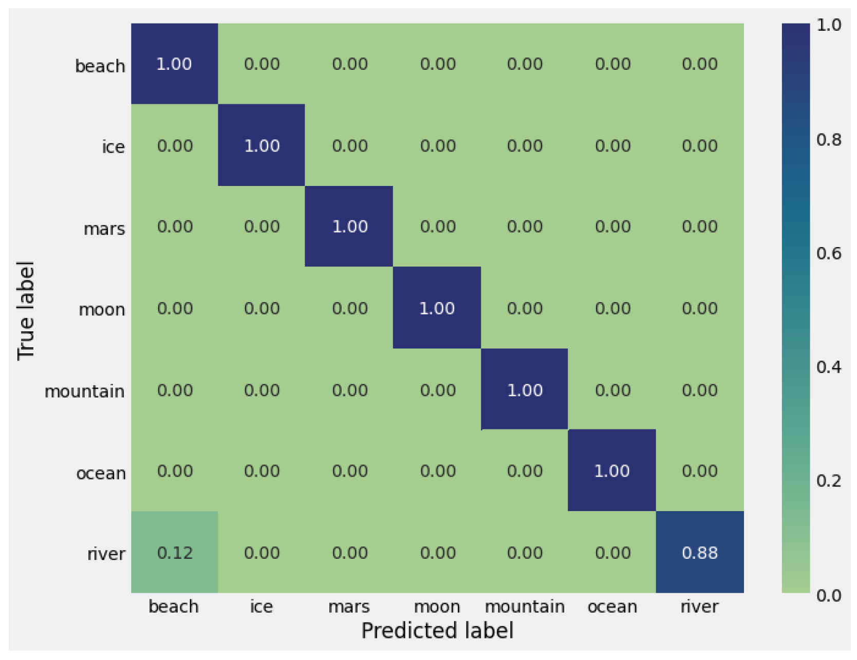
3.1. Satellite Images Dataset

The first dataset named satellite images (retrieved 13 June 2025 from www.kaggle.com/datasets/arjuntyagi25/satellite-images) contained seven classes representing different terrains captured by the satellite. The images in the database were in color and in different sizes. Before being processed by the model, the images were resized to the size of $240\times 240$. The number of samples in the training set was 673, and in the validation, this was set to 46. A total of 10% of the training set was designated as a validation set.

The dataset had a small number of samples assigned to seven classes but with a higher resolution than the second database. The classifier was trained for 100 epochs, during which the accuracy value was recorded on both subsets, similar to the value of the loss function. The results are presented in Figure 4. The first chart shows that the classifier adapted quickly to the training data and achieved accuracy values of over 0.95. However, there are visible jumps in the value up to 0.03 for the first eighty iterations. In the last stages, the training set was classified at the level of 0.98. In contrast, the validation set produced much more divergent results with subsequent iterations. It should be noted that an accuracy level higher than 0.9 was possible after exceeding 63 iterations of the training process. Up to this point, the jumps in values were quite large, and then they fluctuated to around 0.94. The second chart presents the values of the changes in the loss function for both subsets. Based on it, it can be seen that the loss on the training set was minimal and there were no sudden jumps. For the validation set, the loss function reached high values, which stabilized at a minimum level around the 70th iteration. Because of the metric fluctuations, we additionally analyzed their average from five separate runs, which are presented in Figure 5. As can be seen, the rapid changes in the values still remain, but they even out. This indicates that the instability during the training process is related to the nature of the training data. An analysis of the training process best-performing model for this database shows that the proposed classifier model can achieve very high results with such a small number of samples in the sets and a high resolution. The accuracy value for the test set was 0.9783, the precision value was 0.9826, the recall was 0.9783, and the F1-score was calculated as 0.9787. These values confirm the good adaptation of the CNN network to each class. This can also be observed in the confusion matrix (see Figure 6), where only the classification of the sample marked as the river was misclassified.

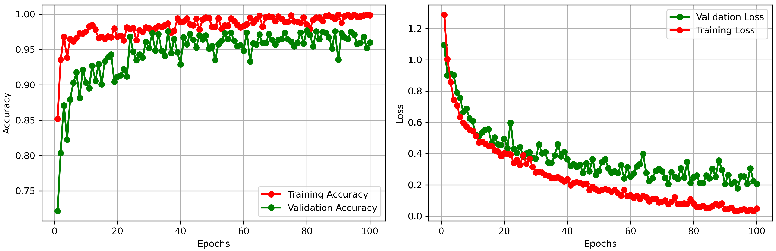
3.2. Visual Terrain Recognition

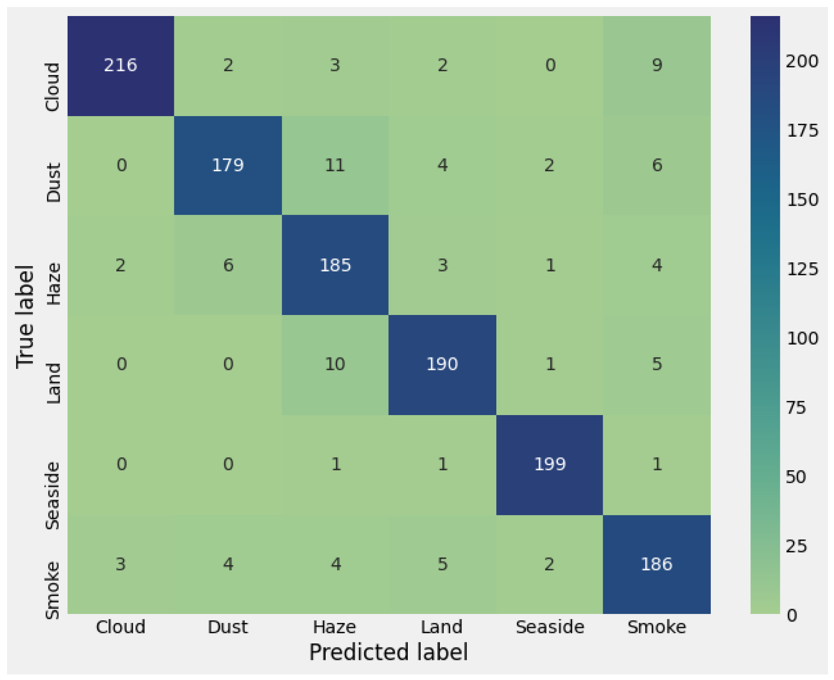
The second dataset named Visual Terrain Recognition (retrieved 13 June 2025 from www.kaggle.com/datasets/shivamguptakaggle/classified-terrain-64x64) was composed of images of size equal to $64\times 64$ and divided into 23 classes. The number of all samples for this dataset in the training set was 303,901. Because of the large quantity of the dataset, we divided the rest of the 37,993 samples into two subsets: validation and test set testing in the proportion of 50:50.

The number of samples is over 300 k, but in a much lower resolution than those in the previous dataset. A total of 30 epochs was enough for the classifier to converge. Charts from the training process are presented in Figure 7. The classifier very quickly achieved high accuracy results of over 0.996 for the training set and 0.994 for the validation set. In both cases, there were no such drastic jumps in values as in the previous database, which is due to the much larger amount of data used in the process of adapting the classifier to all classes. The charts of the loss function for the training set present a rapid decline in value without any major jumps or changes. After only eight epochs, the values of the loss function began to be below 0.15. In the case of the validation set, spikes are visible for the entire training process, ranging between 0.22 and 0.42, which indicates that the classifier obtains low values of the loss function, but they are not as low as for the training set. After completing the full training process, the performance of the classifier was verified on the testing set, which showed a very good match for all classes (see Figure 8). The analysis of the metrics also indicates very good performance of the classifier, as the accuracy was 1.0, the precision was 1.0, and the recall was 1.0, as well as an F1-score of 1.0.

3.3. USTC SmokeRS

The next database used in the research is USTC SmokeRS (Retrieved 13 June 2025 from https://complex.ustc.edu.cn/sjwwataset/list.htm) [30]. The set contains 6225 color photos divided into six classes, such as dust, seaside, smoke, cloud, haze, and land. Images in the database have a size of $256\times 256$. For testing purposes, the database was divided into two subsets: training and validation in the proportion of 80% of the set to 20%. The samples were randomly assigned to both sets. Similar to the satellite dataset, we took 10% of the training set for validation.

The training process was performed for 200 epochs due to the slow increase in the accuracy metric or the decrease in the loss function. During the tests, callbacks were used, which should stop the learning process if the metric values do not change. This situation did not occur because all epochs were completed. The obtained metric results are presented in Figure 9. The classification accuracy metric shows that until training epoch 75, the values on both sets were similar. However, it should be noted that the values determined on the validation set indicate high jumps of up to 0.9. With subsequent learning epochs, the jump values are much smaller. From epoch 75, you can also notice that the values on the validation set are lower than on the training set. At the same time, both metrics are increasing. The loss function values show a downward trend. The loss value curve for the training set finally reaches a loss level of 0.2. In comparison, the loss function values for the test set have higher values despite the decline. The accuracy achieved on the test set was 0.924, with a recall value of 0.926. The precision and F1-score metrics were 0.926 and 0.926, respectively. These results indicate that the classifier is very well adapted to the set. More accurate results are presented in the confusion matrix—Figure 10. The classifier most often failed to provide the correct class for smoke and dust. The most accurate results were for the seaside class, which stood out from the rest of the data in terms of colors and patterns. Despite the lack of a perfect fit to the set, the accuracy of 0.924 indicates the possibility of practical use.

3.4. Discussion

Very good results were obtained for all datasets used in the classifier evaluation. In the case of the first two datasets, the loss function reached a lower value quite quickly. For the third one, the loss function decreased with subsequent epochs, but the difference was small and there were some jumps in the values. The analysis of the accuracy curves also allows us to conclude that the accuracy increases quite quickly and after a certain point, it fluctuates within a certain range. The evaluation results show that the proposed classifier model enabled the extraction of features from images to obtain a good representation of the sample. The model made it possible to pay attention to global and local features at various levels of data processing. This can be further seen in the ablation study presented in

Table 2. Ablation experiments of the proposed modules.

	Satellite Images	Visual Terrain Recognition	USTC SmokeRS
No module	0.9130	0.8691	0.8790
ESA	0.9348	0.9030	0.8742
ESA+MBFA	0.9565	0.9140	0.9046
ESA+MBFA+AFB	0.9783	1.000	0.9240

. Each of the proposed modules contributed to the learning capabilities of the dual-branch CNN network, improving its performance. Furthermore, this trend is visible across all three datasets tested. By applying all of the presented methods combined, the model was able to achieve impressive results. Based on the results obtained, we can conclude that the classifier with the presented data fusion may be an interesting alternative to other existing models used in the classification process. In the context of the modeled framework, this solution may be important due to the possibility of easy supervision over security and potential development through the automation of operations in the cloud and by users.

4. Conclusions

Feature fusion is an element that allows the parallel processing of data by different layers in a CNN. This action allows the network to focus on a larger number of different features and elements of objects presented in the samples. In this paper, we presented a fusion-based CNN model that focuses on spatial features, multi-scale representation, aggregation of global ones, and even searches for patterns. It was achieved by processing the data in parallel through convolutional and pooling layers with different functions and blocks. The CNN model was dedicated to processing satellite images in a framework for terrain analysis. For this purpose, we modeled a solution that maintains data and model security against possible set contamination by validating user data. The proposal was tested on three publicly available databases, where the classifier model showed very good results in adapting to the data. As part of the conducted tests, we evaluated different resolutions of images and the number of classes and samples in datasets. The results point out that the classifier model based on feature fusion allows for obtaining results that can be implemented in practical applications.

References

1. Bai, J.; Zhang, M. RiseNet: Residual Attention-Gated CNNs for Efficient Feature Focus. IEEE Trans. Neural Netw. Learn. Syst. 2025, 36, 567–579. [Google Scholar]
2. Dai, Y.; Liu, F. HDCDF: Hierarchical Dual-Channel Dense Fusion Networks for Fine-Grained Attention. Pattern Recognit. 2025, 142, 109819. [Google Scholar]
3. Wang, L.; Xu, J. TGF-Net: Transformer-Guided Fusion Network for Multi-Source Satellite Image Classification. Remote Sens. Environ. 2025, 303, 113017. [Google Scholar]
4. Chen, Y.; Xia, R.; Yang, K.; Zou, K. MFFN: Image super-resolution via multi-level features fusion network. Vis. Comput. 2023, 40, 489–504. [Google Scholar] [CrossRef]
5. Lee, H.; Park, M. HyFusion: Hybrid CNN-Attention Model for Robust Feature Extraction in Hyperspectral Imaging. Sensors 2025, 25, 987. [Google Scholar]
6. Zhou, T.; He, X. SSFCT: Spectral-Spatial Fusion with Channel-wise Transformers for Hyperspectral Classification. IEEE J. Sel. Top. Appl. Earth Obs. Remote Sens. 2025, 18, 18345–18358. [Google Scholar]
7. Li, Q.; Sun, Z. STNet: Spatio-Temporal Feature Fusion for Satellite Terrain Analysis. In Proceedings of the IEEE/CVF Conference on Computer Vision and Pattern Recognition, Nashville, TN, USA, 19–25 October 2025; pp. 12345–12354. [Google Scholar]
8. Chen, R.; Tan, H. CTANet: Cross-Transformer Attention Network for Remote Sensing Image Segmentation. ISPRS J. Photogramm. Remote Sens. 2025, 202, 32–45. [Google Scholar]
9. Zhou, Z.; Islam, M.T.; Xing, L. Multibranch CNN with MLP-Mixer-Based Feature Exploration for High-Performance Disease Diagnosis. IEEE Trans. Neural Netw. Learn. Syst. 2023, 35, 7351–7362. [Google Scholar] [CrossRef] [PubMed]
10. Hao, Y.; Jing, X.Y.; Chen, R.; Liu, W. Learning enhanced specific representations for multi-view feature learning. Knowl.-Based Syst. 2023, 272, 110590. [Google Scholar] [CrossRef]
11. Hu, T.; Xu, C.; Zhang, S.; Tao, S.; Li, L. Cross-site scripting detection with two-channel feature fusion embedded in self-attention mechanism. Comput. Secur. 2023, 124, 102990. [Google Scholar] [CrossRef]
12. Zhang, Y.; Liang, L.; Mao, J.; Wang, Y.; Jia, L. From Global to Local: A Dual-Branch Structural Feature Extraction Method for Hyperspectral Image Classification. IEEE J. Sel. Top. Appl. Earth Obs. Remote Sens. 2025, 18, 1778–1791. [Google Scholar] [CrossRef]
13. Rowley, A.; Karakuş, O. Predicting air quality via multimodal AI and satellite imagery. Remote Sens. Environ. 2023, 293, 113609. [Google Scholar] [CrossRef]
14. Thomas, M.; Tellman, E.; Osgood, D.E.; DeVries, B.; Islam, A.S.; Steckler, M.S.; Goodman, M.; Billah, M. A framework to assess remote sensing algorithms for satellite-based flood index insurance. IEEE J. Sel. Top. Appl. Earth Obs. Remote Sens. 2023, 16, 2589–2604. [Google Scholar] [CrossRef]
15. Zhao, S.; Liu, M.; Tao, M.; Zhou, W.; Lu, X.; Xiong, Y.; Li, F.; Wang, Q. The role of satellite remote sensing in mitigating and adapting to global climate change. Sci. Total Environ. 2023, 904, 166820. [Google Scholar] [CrossRef] [PubMed]
16. Muhammad, U.; Gao, L. DACN: Dual Attention Convolutional Network for Satellite Terrain Change Detection. Int. J. Appl. Earth Obs. Geoinf. 2025, 126, 103202. [Google Scholar]
17. Bednarek, M.; Nowicki, M.R.; Walas, K. HAPTR2: Improved Haptic Transformer for legged robots’ terrain classification. Robot. Auton. Syst. 2022, 158, 104236. [Google Scholar] [CrossRef]
18. Shaban, A.; Meng, X.; Lee, J.; Boots, B.; Fox, D. Semantic terrain classification for off-road autonomous driving. In Proceedings of the Conference on Robot Learning, PMLR, Auckland, New Zealand, 4–18 December 2022; pp. 619–629. [Google Scholar]
19. Sarinova, A.; Rzayeva, L.; Tendikov, N.; Shayea, I. Simple Implementation of Terrain Classification Models via Fully Convolutional Neural Networks. In Proceedings of the 2023 10th International Conference on Wireless Networks and Mobile Communications (WINCOM), Istanbul, Turkey, 26–28 October 2023; pp. 1–6. [Google Scholar]
20. Wang, W.; Zhang, B.; Wu, K.; Chepinskiy, S.A.; Zhilenkov, A.A.; Chernyi, S.; Krasnov, A.Y. A visual terrain classification method for mobile robots’ navigation based on convolutional neural network and support vector machine. Trans. Inst. Meas. Control. 2022, 44, 744–753. [Google Scholar] [CrossRef]
21. Tamilarasan, K.; Anbazhagan, S.; Ranjithkumar, S. Rock type discrimination using Landsat-8 OLI satellite data in mafic-ultramafic terrain. Geol. Geophys. Environ. 2023, 49, 281–298. [Google Scholar] [CrossRef]
22. Ding, Y.; Zhang, Z.; Zhao, X.; Hong, D.; Cai, W.; Yu, C.; Yang, N.; Cai, W. Multi-feature fusion: Graph neural network and CNN combining for hyperspectral image classification. Neurocomputing 2022, 501, 246–257. [Google Scholar] [CrossRef]
23. Zhang, Y.; Duan, P.; Liang, L.; Kang, X.; Li, J.; Plaza, A. PFS3F: Probabilistic Fusion of Superpixel-wise and Semantic-aware Structural Features for Hyperspectral Image Classification. IEEE Trans. Circuits Syst. Video Technol. 2025, 1. [Google Scholar] [CrossRef]
24. Wang, J.; Huang, Q.; Tang, F.; Meng, J.; Su, J.; Song, S. Stepwise feature fusion: Local guides global. In Proceedings of the International Conference on Medical Image Computing and Computer-Assisted Intervention, Online, 16 September 2022; Springer: Berlin/Heidelberg, Germany, 2022; pp. 110–120. [Google Scholar]
25. Zeng, N.; Wu, P.; Wang, Z.; Li, H.; Liu, W.; Liu, X. A small-sized object detection oriented multi-scale feature fusion approach with application to defect detection. IEEE Trans. Instrum. Meas. 2022, 71, 3507014. [Google Scholar] [CrossRef]
26. Huang, L.; Chen, C.; Yun, J.; Sun, Y.; Tian, J.; Hao, Z.; Yu, H.; Ma, H. Multi-scale feature fusion convolutional neural network for indoor small target detection. Front. Neurorobotics 2022, 16, 881021. [Google Scholar] [CrossRef] [PubMed]
27. Zhou, K.; Zhang, M.; Wang, H.; Tan, J. Ship detection in SAR images based on multi-scale feature extraction and adaptive feature fusion. Remote Sens. 2022, 14, 755. [Google Scholar] [CrossRef]
28. Dong, Y.; Liu, Q.; Du, B.; Zhang, L. Weighted feature fusion of convolutional neural network and graph attention network for hyperspectral image classification. IEEE Trans. Image Process. 2022, 31, 1559–1572. [Google Scholar] [CrossRef] [PubMed]
29. Liang, L.; Zhang, Y.; Zhang, S.; Li, J.; Plaza, A.; Kang, X. Fast Hyperspectral Image Classification Combining Transformers and SimAM-Based CNNs. IEEE Trans. Geosci. Remote Sens. 2023, 61, 5522219. [Google Scholar] [CrossRef]
30. Ba, R.; Chen, C.; Yuan, J.; Song, W.; Lo, S. SmokeNet: Satellite smoke scene detection using convolutional neural network with spatial and channel-wise attention. Remote Sens. 2019, 11, 1702. [Google Scholar] [CrossRef]
Figure 1. Visualization of the proposed framework operation. The satellite data captures an image and sends it for further processing. Clients and clouds are two separate blocks that can communicate using requests and responses. Such a solution allows for maintaining security and real-time operation of the system.
Remotesensing 17 02477 g001
Figure 2. Visualization of the proposed blocks and mechanism in the CNN.
Remotesensing 17 02477 g002
Figure 3. Visualization of the proposed structure of the classifier.
Remotesensing 17 02477 g003
Figure 4. Classifier training analysis plots for the first dataset—satellite images. From the left: accuracy plot and loss function value plot. (Best-performing model).
Remotesensing 17 02477 g004
Figure 5. Average (5 runs) training accuracy and loss plots during training for the first dataset—satellite images. From the left: accuracy plot and loss function value plot.
Remotesensing 17 02477 g005
Figure 6. Confusion matrix for the first dataset—satellite images.
Remotesensing 17 02477 g006
Figure 7. Classifier training analysis plots for the second dataset—Visual Terrain Recognition. From the left: accuracy plot and loss function value plot.
Remotesensing 17 02477 g007
Figure 8. Confusion matrix for the second dataset—Visual Terrain Recognition.
Remotesensing 17 02477 g008
Figure 9. Classifier training analysis plots for the third dataset—USTC SmokeRS. From the left: accuracy plot and loss function value plot.
Remotesensing 17 02477 g009
Figure 10. Confusion matrix for the third dataset—USTC SmokeRS.
Remotesensing 17 02477 g010