A Radar-Based Fast Code for Rainfall Nowcasting over the Tuscany Region

Abstract

Accurate short-term precipitation forecasting (nowcasting) based on weather radar data is essential for managing weather-related risks, particularly in applications such as airport operations, urban flood prevention, and public safety during outdoor events. This study proposes a computationally efficient nowcasting method based on a Lagrangian advection scheme, estimating both the translation and rotation of radar-observed precipitation fields without relying on machine learning or resource-intensive computation. The method was tested on a two-year dataset (2022–2023) over Tuscany, using data collected from the Italian Civil Protection Department’s radar network. Forecast performance was evaluated using the Critical Success Index (CSI) and Mean Absolute Error (MAE) across varying spatial domains (1° × 1° to 2° × 2°) and precipitation regimes. The results show that, for high-intensity events (average rate > 1 mm/h), the method achieved CSI scores exceeding 0.5 for lead times up to 2 h. In the case of low-intensity rainfall (average rate < 0.3 mm/h), its forecasting skill dropped after 20–30 min. Forecast accuracy was shown to be highly sensitive to the temporal stability of precipitation intensity. The method performed well under quasi-stationary stratiform conditions, whereas its skill declined during rapidly evolving convective events. The method has low computational requirements, with forecasts generated in under one minute on standard hardware, and it is well suited for real-time application in regional meteorological centres. Overall, the findings highlight the method’s effective balance between simplicity and performance, making it a practical and scalable option for operational nowcasting in settings with limited computational capacity. Its deployment is currently being planned at the LaMMA Consortium, the official meteorological service of Tuscany.

1. Introduction

Short-term precipitation forecasting by radar, commonly referred to as radar nowcasting, is a critical tool in modern meteorology, particularly for managing the societal risks associated with intense and localised weather events. These forecasts, typically spanning from a few minutes up to several hours, are essential for anticipating rainfall and mitigating its impacts across a wide range of domains: flood prevention in urban environments, safe air traffic control at airports, and the real-time coordination of large outdoor public events. In high-impact scenarios, accurate and timely nowcasting is indispensable, enabling early warning dissemination and supporting rapid, time-sensitive decision-making in emergency management.

To meet these needs, the scientific community has made significant progress in improving radar-based rainfall monitoring and forecasting systems. Advanced techniques for merging radar and rain gauge data have led to better quantitative precipitation estimation, thereby enhancing the reliability of radar-derived forecasts [1]. Regional radar networks, especially those operating in the X-band, have extended both coverage and resolution, improving rainfall detection in complex orographic regions, such as central Italy [2]. Additional efforts, focused on recalibrating cumulative precipitation estimates over large spatial domains, have further strengthened long-term hydrometeorological monitoring [3], while the integration of radar mosaics into multi-sensor frameworks has enabled more comprehensive regional-scale rainfall analysis [4].

In recent years, substantial progress has also been made in exploring alternative data sources to complement radar systems. Several innovative approaches have emerged, including the use of opportunistic microwave signal measurements, which exploit commercial or satellite microwave communication links as indirect sensors of rainfall intensity [5,6,7,8,9,10,11,12,13]. These methods are especially valuable in areas lacking dense radar coverage and offer new possibilities for distributed, real-time monitoring.

Meanwhile, major advancements in machine learning, particularly in the field of deep neural networks, have expanded the toolkit available for nowcasting. These models are capable of classifying precipitation types (e.g., stratiform vs. convective), identifying complex spatial and temporal patterns, and improving forecast skill beyond traditional methods [14,15,16]. Deep learning-based classification methods are often used for preprocessing before applying probabilistic or deterministic forecasting techniques.

However, despite these innovations, practical challenges remain. Many machine learning-based systems are computationally intensive and require large, curated datasets for training resources that are not always available to operational meteorological centres. Additionally, such models often show limited generalisation across different climatic and geographic regions, requiring frequent retraining to maintain acceptable accuracy.

This situation underscores the need for nowcasting approaches that combine predictive performance with computational simplicity [17,18,19,20,21,22,23], making them deployable in real-time operations, even under limited infrastructure.

To address this gap, our study proposes a computationally efficient and easily transferable nowcasting method, building on the deterministic Lagrangian advection framework described by Ayzel et al. [17].

Radar-based nowcasting techniques can generally be grouped into three categories, depending on the characteristics of the precipitation field [24]:

• Climatology-based approaches;
• Observation-based methods relying on the latest rainfall measurements;
• Lagrangian methods, which assume that the motion and intensity of precipitation remain persistent over short time intervals [24,25].

Among these, Lagrangian approaches offer a promising balance between accuracy and computational demand. They typically consist of two phases: tracking and prediction (or extrapolation) [26]. First, the velocity field of the precipitation is estimated from consecutive radar images; this velocity field is then used to extrapolate the precipitation field forward in time beyond the latest observation.

Our implementation emphasises operational usability and low resource requirements. The method requires no training datasets, classification schemes, or machine learning infrastructure. It has been successfully tested on standard desktop hardware (Intel Core i5, 8 GB RAM, no GPU), with each forecast cycle completed in less than one minute. This rapid performance highlights the method’s suitability for deployment in regional meteorological services with limited computational capacity.

The procedure was specifically tested in the Tuscany region, as it is intended to be adopted by the LaMMA Consortium, the official meteo-oceanografic service of Tuscany, for operational weather alert management. To evaluate its performance, we applied the method to a two-year dataset (2022–2023) of radar observations from the Italian Civil Protection Department’s national radar network.

We assessed forecast accuracy over various spatial domains, from small local areas to broader regional scales, and under different precipitation regimes, including both stratiform and convective events. This multi-scale evaluation was designed to ensure robustness across real-world operational conditions.

In summary, this study demonstrates that a simple, fast, and scalable radar nowcasting approach can meet the operational needs of public weather services. The method provides a practical alternative to machine learning-based techniques and offers reliable short-term forecasts that are compatible with modest infrastructure, thereby enhancing regional preparedness for rainfall-related hazards.

2. Materials and Methods

2.1. The Nowcasting Technique

The rainymotion library [17] is a state-of-the-art open-source Python package designed for the development, evaluation, and operational implementation of radar-based precipitation nowcasting techniques. It was specifically developed based on methods that rely on the Lagrangian persistence assumption, according to which precipitation intensity remains approximately constant over short time horizons, allowing for the extrapolation of the precipitation field through motion estimation. The rainymotion package provides not only the algorithmic core, but also preprocessing tools, evaluation metrics, and visualisation utilities, making it suitable for both research and real-time applications.

The full source code is freely available through GitHub (version: rainymotion-0.1) and is complemented by comprehensive documentation (https://rainymotion.readthedocs.io, accessed on 10 January 2024), which includes detailed installation guidelines, methodology descriptions, and illustrative usage examples.

The library implements four main nowcasting schemes—SparseSD, Sparse, Dense, and DenseRotation—which can be categorised into two methodological families: sparse and dense motion estimation approaches. While all methods share the same core assumption of short-term Lagrangian persistence, they differ in how motion is estimated and how the precipitation field is subsequently extrapolated.

The sparse models are as follows:

• SparseSD utilises only the two most recent radar images to estimate motion vectors and produce forecasts. This method is especially computationally efficient and ideal for rapid deployments.
• Sparse builds on a longer radar image history—typically the last 24 frames—to identify persistent rainfall features and filter out transient noise. It improves the robustness of the motion estimation at the cost of slightly increased computation.

Both sparse methods are lightweight and well suited for detecting and tracking discrete, well-defined precipitation cells. However, their performance tends to degrade in cases of homogeneous or weakly structured rainfall patterns, where motion estimation becomes less reliable due to a lack of strong gradients or textures in the radar reflectivity field [17].

The dense models address these limitations by computing motion vectors for every pixel in the radar image using the Dense Inverse Search (DIS) optical flow algorithm, proposed by Kroeger et al. [27]. This enables a more complete and continuous description of the motion field, allowing the models to capture fine-scale dynamics and subtle deformation patterns that are especially relevant in convective systems, as follows:

• In the Dense scheme, the estimated motion vectors are directly applied in a constant-vector advection scheme, where each pixel is displaced in the direction of its motion vector at each lead time step.
• The DenseRotation scheme, by contrast, optimises the advection process by fitting a global affine transformation to the velocity field—combining translation, rotation, and scaling—and applying it uniformly to the precipitation field. This approach is less sensitive to local noise and can capture larger-scale structural motion, such as the rotation or expansion/contraction of rain systems [24].

In a set of preliminary tests conducted using data from the Italian Civil Protection Department’s radar network (DPCN), all four methods were evaluated across a variety of meteorological conditions. The DenseRotation method consistently achieved superior forecast accuracy for both stratiform and convective precipitation, across different rainfall intensities and spatial domains. These findings are aligned with those reported by Ayzel et al. [17], who also identified DenseRotation as the most effective among the rainymotion methods.

While DenseRotation is more computationally demanding than the other three schemes, our testing confirmed that it can still be executed efficiently on standard desktop hardware. In this study, forecasts were generated on a workstation equipped with an Intel Core i5 processor, 8 GB of RAM, and no dedicated GPU, with total processing time for each nowcast remaining below 60 s. This makes it a viable option for real-time operational use, even in settings with limited computational resources.

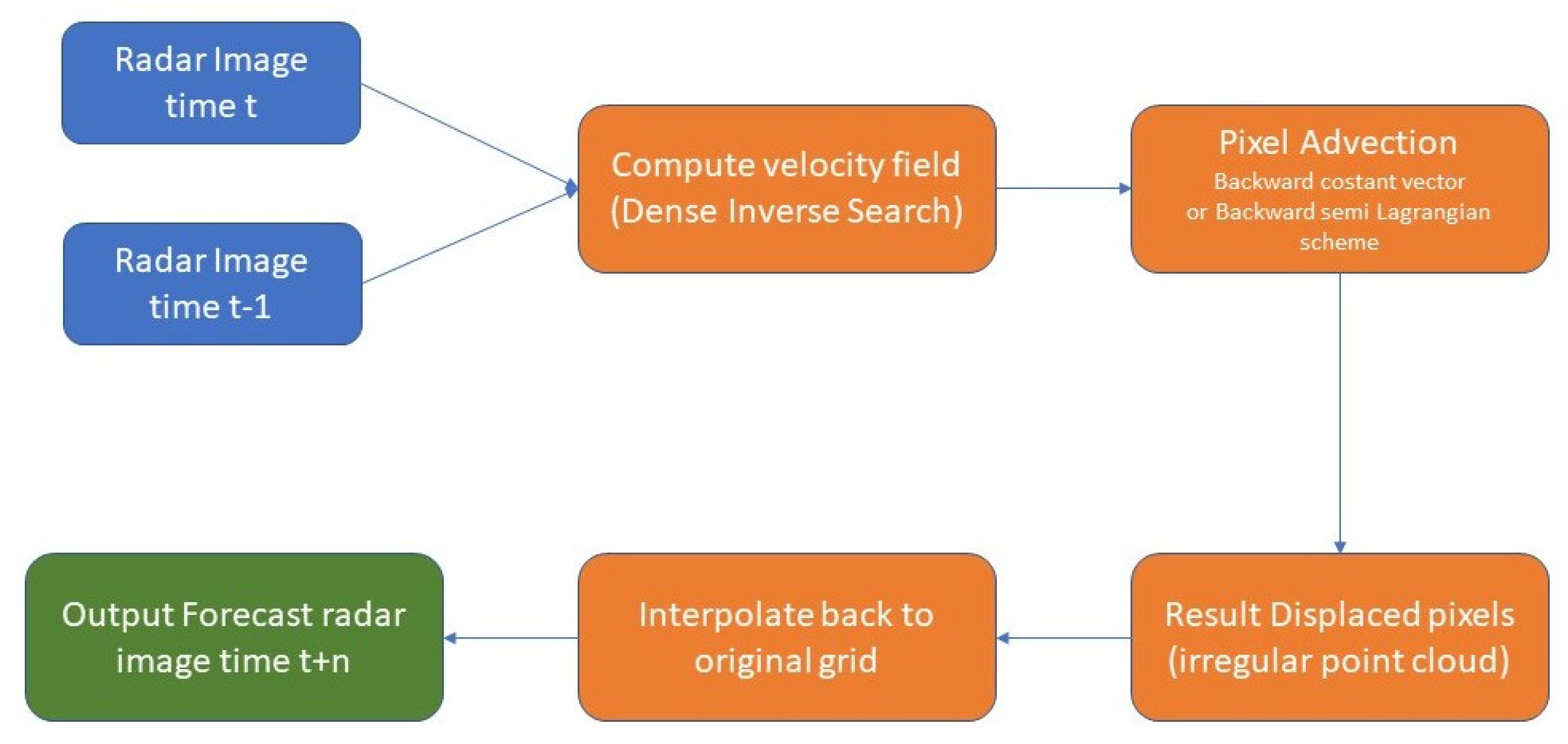
The main computational steps in the DenseRotation workflow are as follows:

• Velocity field estimation: The DIS algorithm is applied to two consecutive radar images (at times t–1 and t) to derive a dense field of motion vectors.
• Pixel advection: Each pixel in the radar image is advected forward using a semi-Lagrangian scheme [24]. This scheme updates the velocity at each prediction step t + n using linear interpolation of the surrounding motion vectors to ensure accurate and smooth displacement paths.
• Interpolation to radar grid: After advection, the resulting pixel positions form a non-uniform cloud. Their intensities are projected back onto the regular radar grid using inverse distance weighting. To preserve the integrity of the precipitation structures and avoid excessive smoothing, this interpolation is executed only once, after the entire advection process, as recommended in the “interpolate once” approach [24].

This technique preserves fine-scale spatial structures and ensures a physically consistent evolution of the precipitation field over short lead times. A schematic flowchart (Figure 1) illustrating the DenseRotation procedure is provided in the following figure.

2.2. Evaluation Method

In order to quantitatively assess the performance of precipitation nowcasting, we evaluated the results using two statistical indices commonly used in the literature [28,29].

The Critical Success Index (CSI) is defined as follows:

$$CSI={\displaystyle \frac{Hits}{Hits+False alarms+Misses}},$$

(1)

where hits represent correctly predicted events, false alarms are false positives (predicted events that did not occur), and misses are false negatives (events that occurred but were not predicted by the procedure). Hits, false alarms, and misses are determined based on a predetermined threshold. Following the studies by Bowler [30] and Foresti [31], a threshold of 1 mm/h was applied to the rain rate for calculating the CSI. The procedure for evaluating the CSI is also provided within the rainymotion library. Compared to other quantitative metrics, the CSI can accurately assess the predictive model by capturing the essence of temporal evolution, partially reproducing the human capacity to qualitatively evaluate the goodness of nowcasting. Its value provides a measure of the forecasting accuracy, with higher values indicating better predictions. A CSI value of one indicates a perfect match between the forecasting and the event that occurred.

The Mean Absolute Error (MAE) is defined as follows:

$$MAE={{\displaystyle \sum }}_{i=1}^N{\displaystyle \frac{\left|M_i-P_i\right|}{N}},$$

(2)

where M_i and P_i are the measure and the prediction of the rain rate in the i-th pixel of the corresponding observation, and N is the total number of pixels.

2.3. Radar Network

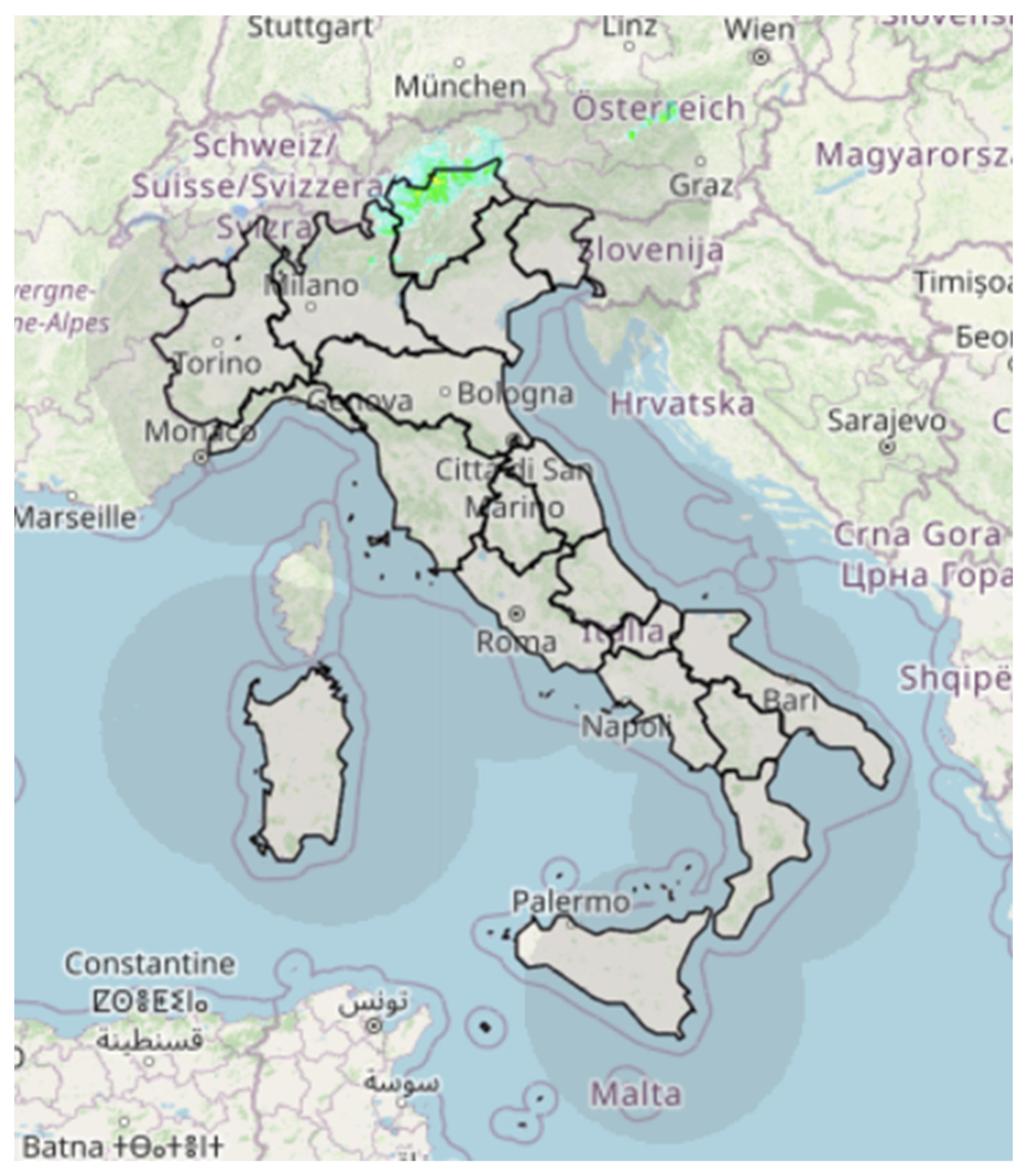
The radar products used in this study were provided by the Italian Civil Protection Department (DPC) through the Radar-DPC platform [32]. Figure 2 shows the actual radar coverage over Italian territory. The data are freely accessible [33]. The platform allows for the nationwide visualisation of both ongoing and recorded weather phenomena in the last 24 h. This is achieved through the real-time processing of raw data from the national radar network, the network of rain gauge and thermometric stations for the Regional Hydrological Service of the Tuscany Region, satellite data, and the lightning network. The production of these data involves the Italian regions, along with the DPC, through the Functional Centres Network, Enav (the National Flight Assistance Agency), and the Italian Air Force.

Radar-DPC is based on the WIDE (Weather Ingestion Data Engine) software platform, specifically designed for the execution of automatic data collection processes and the publication of parameterised web services that can be invoked by any WMS/WMTS client. Temporal series of product samples can be requested and displayed, whether they are monitoring data or forecast model outcomes.

The precipitation-related products provided by the Radar-DPC include the following:

VMI (Vertical Maximum Intensity), updated every 5 min. This product gives the maximum reflectivity value [dBZ] present on the vertical at each point. VMI is used for general monitoring, allowing for the identification of areas where significant weather phenomena are occurring and classifying them based on their type (fronts, convective systems).

SRI (Surface Rainfall Intensity), updated every 5 min. This product is processed through specific operational chains developed at the CFC (Central Functional Centre), combining data from the radar network with those from the rain gauge network. Its goal is to provide an estimate of ground precipitation intensity [mm/h]. This is the product used in the present study.

SRT_1 (cumulative precipitation in 1 h), updated every 5 min. SRT_1 provides the cumulative precipitation [mm] in the last hour, based on the integration of the radar SRI data over 1 h and ground rain gauge network data.

The image pixels have a horizontal resolution of 0.01° in both latitude and longitude.

3. Results

The performance of the nowcasting technique was assessed over the Tuscany region (central Italy), which was chosen as a representative area due to the availability of high-resolution radar data and the presence of diverse precipitation regimes, including convective, stratiform, and mixed types. Nevertheless, the proposed methodology is generalisable and can be applied to any region covered by weather radar.

For this analysis, we used the Surface Rainfall Intensity (SRI) radar product provided by the Italian Civil Protection Department (DPC). This dataset has a spatial resolution of 0.01° × 0.01° and a temporal resolution of 5 min, covering the period from 1 January 2022 to 31 December 2023. These features allow for accurate tracking of the spatial and temporal evolution of precipitation events.

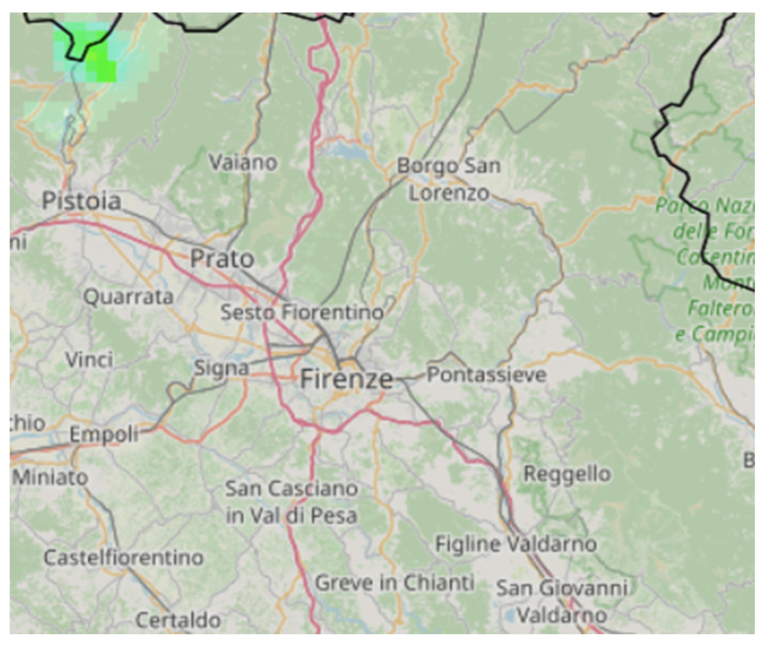
To investigate the influence of domain size on nowcasting accuracy, the procedure was applied to square domains of 1°, 1.5°, and 2°, centred at 43.75°N, 11.25°E (see Figure 3). This multi-domain setup enables the evaluation of model sensitivity to spatial context, particularly regarding forecast skill variations caused by edge effects, partial precipitation coverage, and motion field stability.

To evaluate the capability of the methodology in nowcasting rainfall events, we analysed all episodes (see

Table 1. Characteristics of all analysed events for each of the three selected domains: initial and end time, duration [hours], maximum average rain rate [mm/h] and the normalised percentage of pixels with a rain rate > 1 mm/h.

Event n	Initial Time	End Time		1° × 1°		1.5° × 1.5°		2° × 2°
			T(h)	Avg_RR Max (mm/h)	FNP Max	Avg_RR Max (mm/h)	FNP Max	Avg_RR Max (mm/h)	FNP Max
1	5/1/22 11.00	6/1/22 2.00	15.0	5.11	0.88	3.94	0.81	3.12	0.7
2	9/1/22 2.00	9/1/22 14.00	12.0	2.55	0.67	2.32	0.63	1.64	0.52
3	14/2/22 5.00	14/2/22 16.00	11.0	1.22	0.33
4	15/2/22 1.00	15/2/22 15.00	14.0	1.6	0.44	1.11	0.31	0.88	0.26
5	25/2/22 16.00	26/2/22 3.00	11.0	2.37	0.66	2.48	0.56	2.47	0.54
6	30/3/22 4.00	31/3/22 17.00	37.0	1.55	0.38	1.91	0.42	2.65	0.47
7	2/4/22 0.00	2/4/22 16.00	16.0	1.07	0.37	0.95	0.29	0.93	0.22
8	20/4/22 22.00	22/4/22 11.00	37.0	2.65	0.57	1.85	0.51	1.64	0.5
9	24/4/22 6.00	24/4/22 21.00	15.0	2.24	0.47	1.35	0.29	1.04	0.22
10	5/5/22 12.00	6/5/22 8.00	20.0	1.77	0.68	1.34	0.52	1.1	0.44
11	12/8/22 17.00	13/8/22 5.00	12.0	2.2	0.42	1.47	0.28	1	0.22
12	15/8/22 16.00	16/8/22 2.00	10.0	4.7	0.49	2.85	0.29	1.78	0.2
13	18/8/22 6.00	19/8/22 5.00	23.0	6.36	0.41	3.86	0.35	4.12	0.34
14	3/9/22 5.00	3/9/22 15.00	10.0	3.02	0.59	1.71	0.37	1.44	0.31
15	15/9/22 1.00	15/9/22 9.00	8.0	0.41	0.042	0	0	0	0
16	17/9/22 5.00	17/9/22 16.00	11.0	2.24	0.53	2.55	0.49	2.74	0.47
17	24/9/22 10.00	25/9/22 3.00	17.0	3.85	0.78	2.9	0.66	2.4	0.57
18	29/9/22 5.00	30/9/22 23.00	42.0	3.42	0.71	2.42	0.51	1.78	0.36
19	3/11/22 20.00	4/11/22 6.00	10.0	3.56	0.5	2.86	0.42	2.21	0.36
20	10/11/22 1.00	10/11/22 16.00	15.0	0.59	0.24	0.32	0.12	0.2	0.07
21	15/11/22 7.00	16/11/22 17.00	34.0	1.31	0.49	1.16	0.45	1.11	0.41
22	17/11/22 20.00	18/11/22 12.00	16.0	0.89	0.22	0.42	0.11	0.31	0.07
23	19/11/22 8.00	19/11/22 23.55	15.9	2.08	0.73	1.27	0.51
24	21/11/22 11.00	22/11/22 23.55	36.9	4.83	0.94	2.86	0.9	2.46	0.8
25	25/11/22 9.00	26/11/22 3.00	18.0	2.45	0.71	1	0.35
26	3/12/22 0.00	3/12/22 23.55	23.9	1.32	0.55
27	4/12/22 19.00	6/12/22 3.00	32.0	2.27	0.53
28	8/12/22 11.00	11/12/22 18.00	79.0	2.54	0.64	1.73	0.5	1.71	0.42
29	15/12/22 9.00	17/12/22 7.00	46.0	3.29	0.9	2.81	0.8	2.76	0.75
30	8/1/23 18.00	9/1/23 6.00	12.0	3.06	0.57	2.05	0.53	1.76	0.48
31	16/1/23 14.00	19/1/23 19.00	77.0	3.36	0.83	2.92	0.7	2.53	0.63
32	25/2/23 16.00	26/2/23 19.00	27.0	2.44	0.71	1.92	0.62	2.03	0.56
33	1/3/23 5.00	1/3/23 16.00	11.0	2.9	0.82	0.44	0.17	0.71	0.24
34	10/3/23 0.00	10/3/23 11.00	11.0	0.9	0.17	0.6	0.12	0.45	0.09
35	14/3/23 6.00	14/3/23 22.00	16.0	0.54	0.16	0.34	0.1	0.45	0.09
36	19/3/23 14.00	20/3/23 8.00	18.0	3.12	0.81	2.4	0.69	1.83	0.56
37	7/4/23 14.00	8/4/23 9.00	19.0	1.71	0.39	1.21	0.34	1.09	0.29
38	10/5/23 0.00	10/5/23 20.00	20.0	2.06	0.77	1.8	0.63	1.88	0.6
39	13/5/23 10.00	13/5/23 16.00	6.0	0.9	0.28	0.88	0.26	0.75	0.21
40	4/6/23 18.00	5/6/23 11.00	17.0	0.85	0.3	0.7	0.23	0.59	0.19
41	29/8/23 13.00	29/8/23 19.00	6.0	0.28	0.076	0.3	0.07	0.31	0.07
42	18/10/23 5.00	18/10/23 17.00	12.0	0.7	0.25	0.68	0.24	0.76	0.22
43	21/10/23 9.00	21/10/23 20.30	11.5	2.2	0.51	1.44	0.35	1.2	0.27
44	24/10/23 8.00	25/10/23 2.00	18.0	4.52	0.87	3.61	0.66	3.17	0.55
45	30/10/23 18.00	31/10/23 2.00	8.0	0.94	0.16	0.77	0.15	0.52	0.11
46	2/11/23 13.30	3/11/23 6.00	16.5	8.95	0.99	7.71	0.97	6.33	0.9
47	4/11/23 18.00	5/11/23 7.00	13.0	3.51	0.6	2.34	0.51	1.75	0.41
48	9/11/23 16.00	11/11/23 8.30	40.5	2.94	0.45	2.65	0.37	1.77	0.28
49	27/11/23 20.00	28/11/23 7.00	11.0	0.61	0.21	0.59	0.18	0.6	0.17
50	30/11/23 4.00	30/11/23 19.00	15.0	0.53	0.17	0.31	0.09	0.2	0.06
51	2/12/23 2.00	2/12/23 16.00	14.0	3.71	0.66	2.25	0.48	1.58	0.36
52	4/12/23 11.00	5/12/23 17.00	30.0	2.91	0.78	2.6	0.67	2.03	0.6
53	14/12/23 8.00	14/12/23 15.00	7.0	0.21	0.07	0.3	0.07	0.49	0.1

and Figure 4) with average rain rates (Avg_RR) exceeding 0.5 mm/h at peak intensity, where Avg_RR is defined as the mean rain rate across all pixels within the domain at a given time. This threshold captures a variety of meteorological conditions, from intense, localised convective events to more widespread, lower-intensity stratiform systems. Each event was analysed from its initiation through dissipation, including periods of low rainfall intensity.

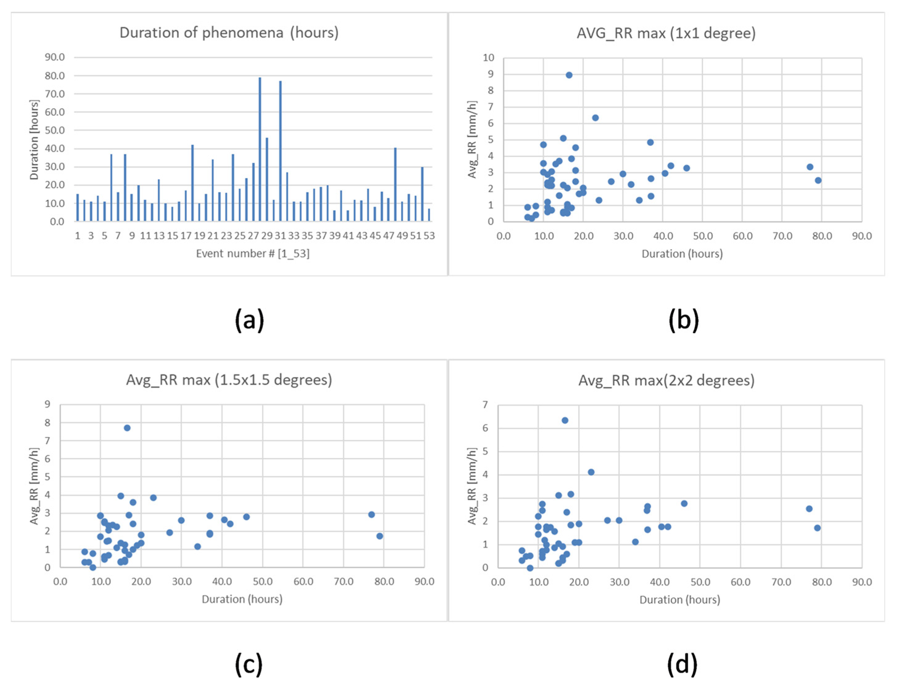
Table 1 summarises key event characteristics, including duration, maximum Avg_RR, and the Fraction of Notable Pixels (FNP), defined as the normalised percentage of pixels exceeding a 1 mm/h rain rate. FNP serves as a proxy for the spatial extent of each event. Figure 4 displays the distribution of event durations and its relationship to average intensity, offering insights into the temporal and structural variability of the studied systems.

Most events (over 90%) lasted more than 10 h, and approximately 30% extended beyond 20 h. Following Stein and Hewson [34,35], a fixed threshold of the Critical Success Index (CSI) equal to 0.5 was adopted as a benchmark for acceptable forecast skill. This value corresponds to a hit rate of 50% and is widely recognised as a practical threshold for operational reliability.

Accordingly, we defined the maximum acceptable values for the Mean Absolute Error (MAE) in reference to the 0.5 CSI benchmark. Our analysis showed that forecast performance is generally more reliable when the mean precipitation intensity remains stable during the event.

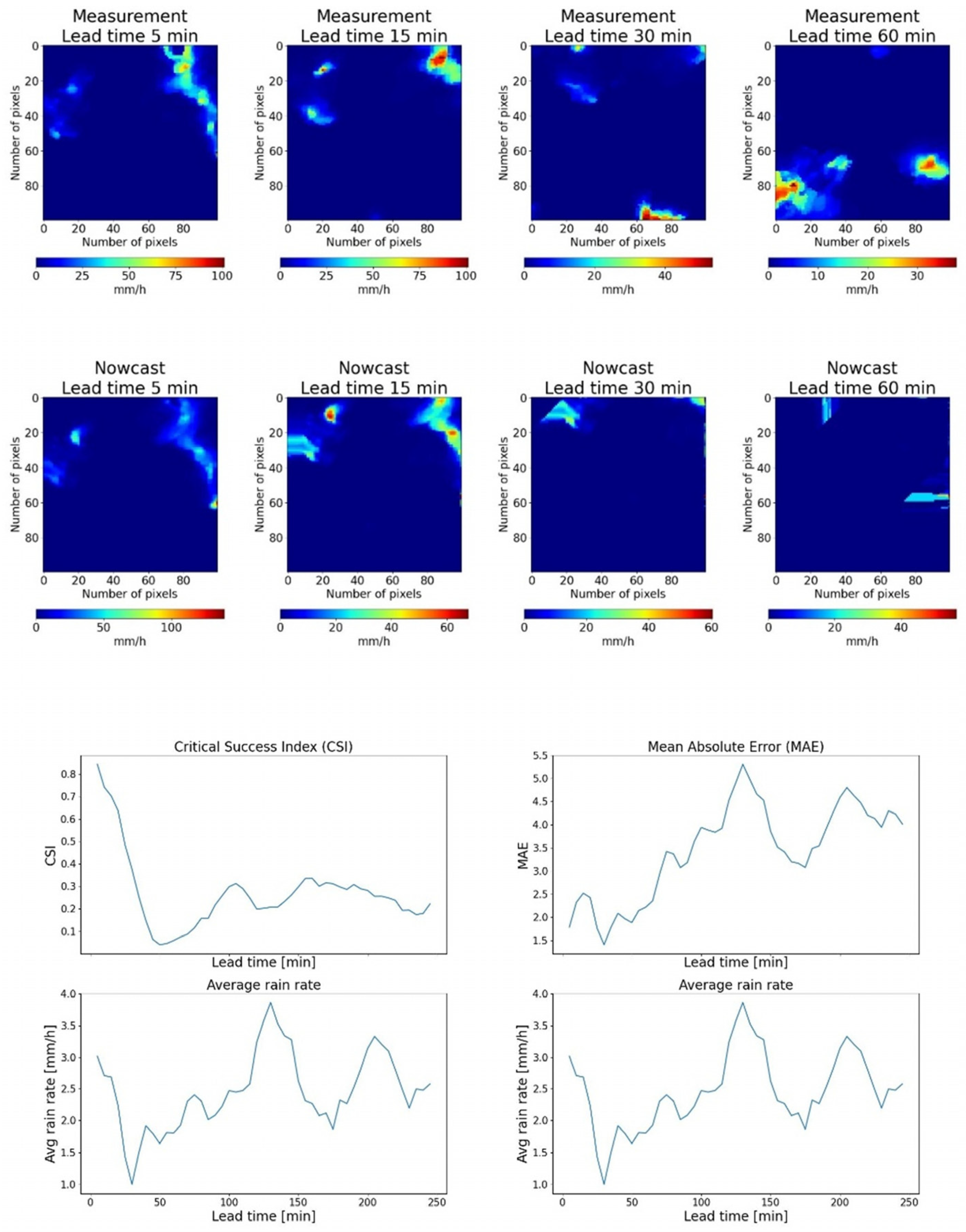
The analysis results indicate that nowcasting performance is generally more reliable when the mean precipitation intensity exhibits limited variation throughout the duration of the event. This outcome is consistent with the core assumption of the nowcasting algorithm, which relies on the near-constancy of total precipitation within the domain over short time horizons. However, since the method is entirely deterministic, it lacks the flexibility to adapt to evolving meteorological conditions that can lead to significant changes in rainfall intensity. As a result, forecast accuracy tends to decline in scenarios where rapid or substantial variations occur, such as those induced by synoptic-scale systems or the rapid development of convective activity. This limitation is clearly illustrated in the example shown in Figure 5, where a significant violation of the precipitation persistence assumption leads to a rapid deterioration in nowcasting skill.

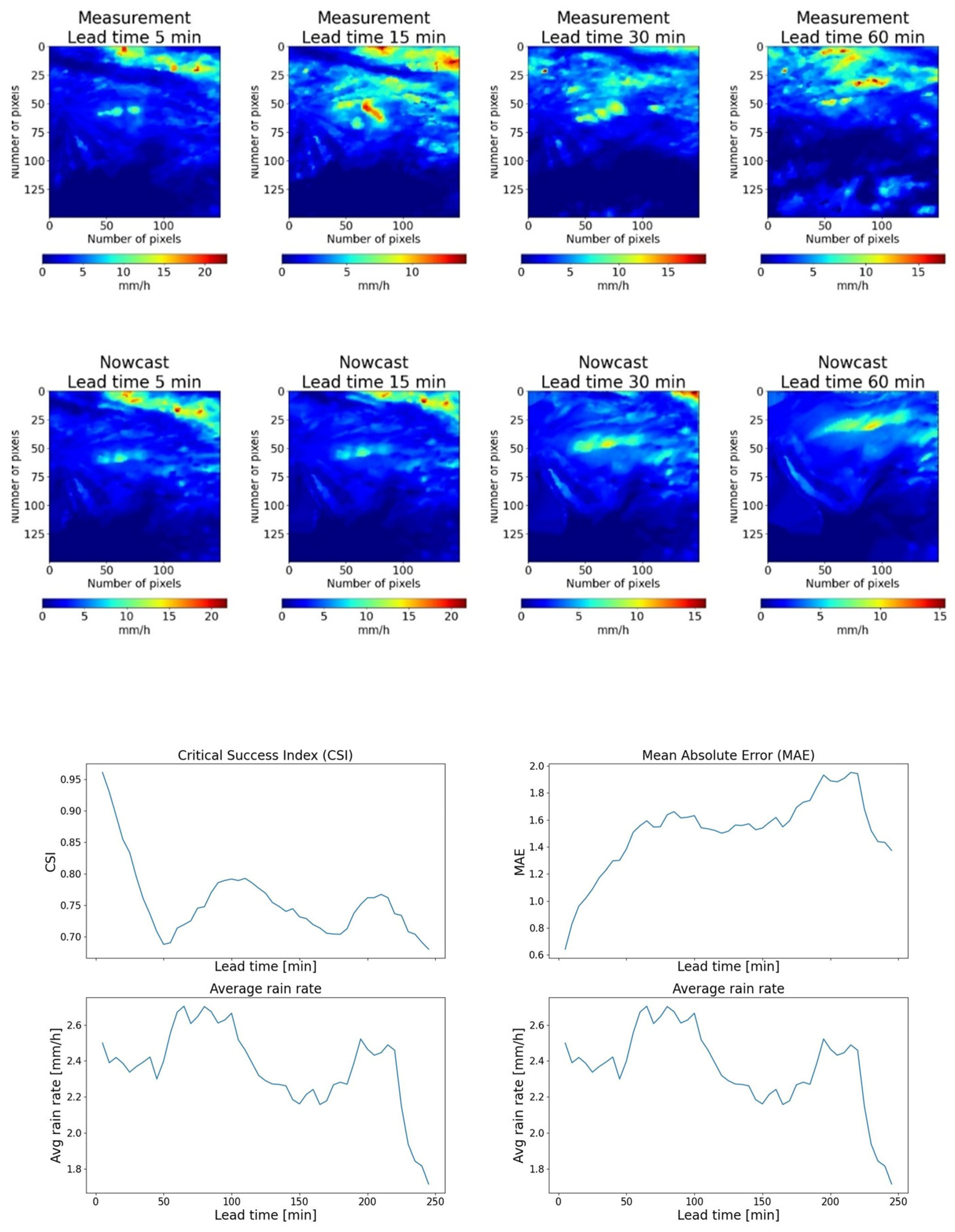
Conversely, the case shown in Figure 6 featuring approximately 70 min of sustained precipitation with low variation demonstrates more stable and consistent nowcasting accuracy within this window, highlighting the importance of event persistence in model performance.

3.1. Analysis of the Performances of Nowcasting

This section analyses the performance of the implemented nowcasting algorithm with respect to key parameters. The evaluation is based on the previously defined statistical indices (CSI and MAE) and focuses on their variation over the forecast horizon. The results show that nowcasting accuracy is primarily affected by lead time and the average precipitation intensity within the selected domain. Additionally, the algorithm’s performance is assessed under different precipitation regimes, with particular attention given to stratiform and convective conditions.

3.1.1. Dependence of Nowcasting Accuracy on Lead Time

The analysis of the average accuracy of nowcasting as a function of lead time was performed considering all phenomena in the selected period for various rainfall regimes and precipitation rates. The results quantify the expected decrease in nowcasting accuracy with increasing lead time. It was observed that the MAE thresholds—below which nowcasting can be considered sufficiently accurate—increase with higher average rain rates, as the relative error becomes smaller.

Notably, the accuracy of nowcasting appears to be approximately independent of the spatial extent of the selected domain.

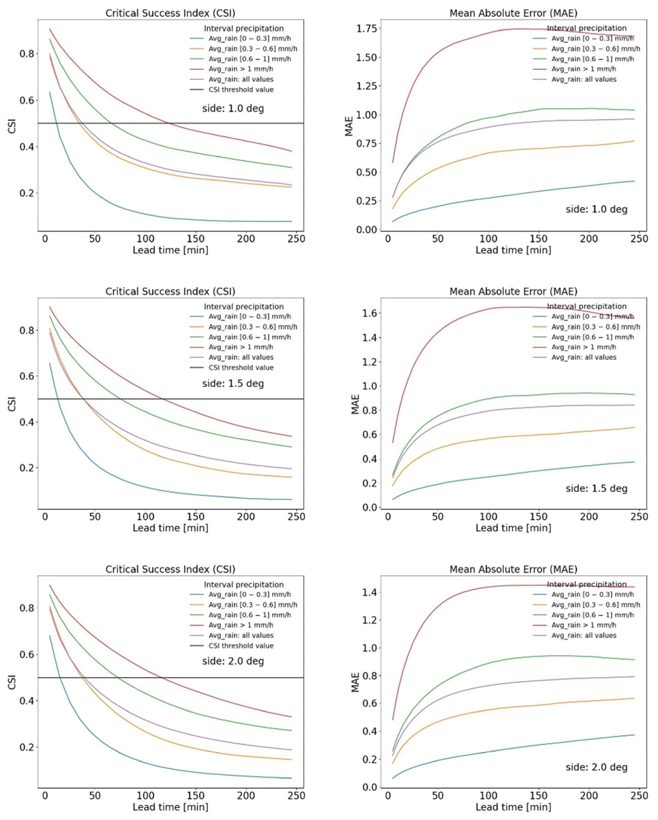
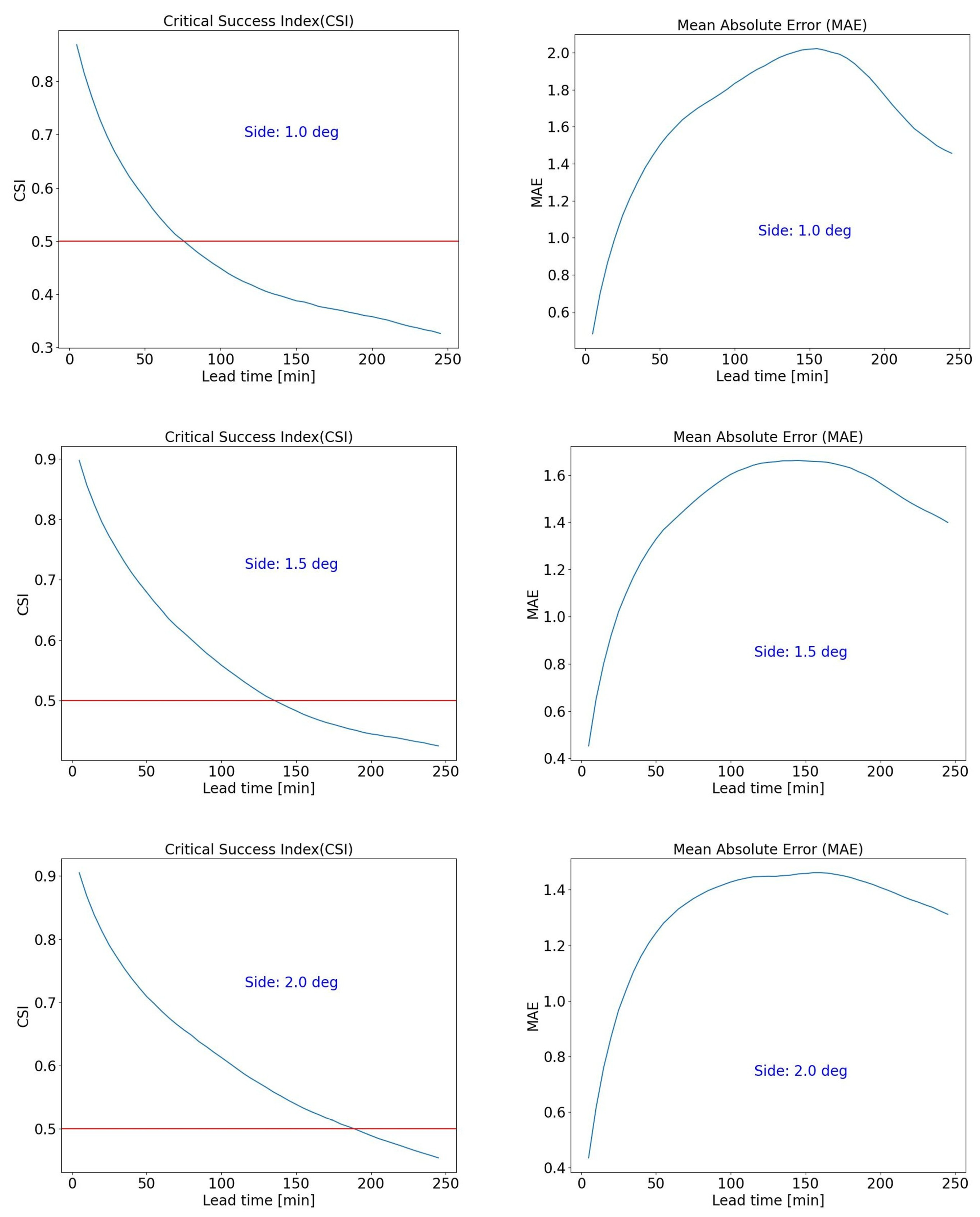
As shown in Figure 7, for low rainfall regimes (0 mm/h < RR_avg < 0.3 mm/h), acceptable forecast accuracy is maintained for lead times of up to approximately 20 min. For moderate rainfall (0.3 mm/h < RR_avg < 0.6 mm/h), this duration extends to around 40 min. In the case of heavy rainfall (0.6 mm/h < RR_avg < 1 mm/h), accurate forecasts can be sustained for about 70 min. Finally, for very heavy rainfall (RR_avg > 1 mm/h), the lead time extends to approximately 105 min.

The corresponding MAE threshold values identified for low, moderate, heavy, and very heavy rainfall regimes are 0.15, 0.5, 0.95, and 1.68, respectively (see Figure 7).

It is worth noting that, in terms of MAE, as nowcasting accuracy progressively degrades with increasing lead time, the metric tends to stabilise, exhibiting an almost asymptotic behaviour. This phenomenon is attributed to the gradual loss of correlation between observed and forecasted precipitation fields, which makes the MAE values at successive lead times nearly indistinguishable. Under such conditions, the index becomes primarily influenced by the average precipitation intensity, rather than by the forecast lead time.

3.1.2. Dependence of Nowcasting Accuracy on Average Rain Rate

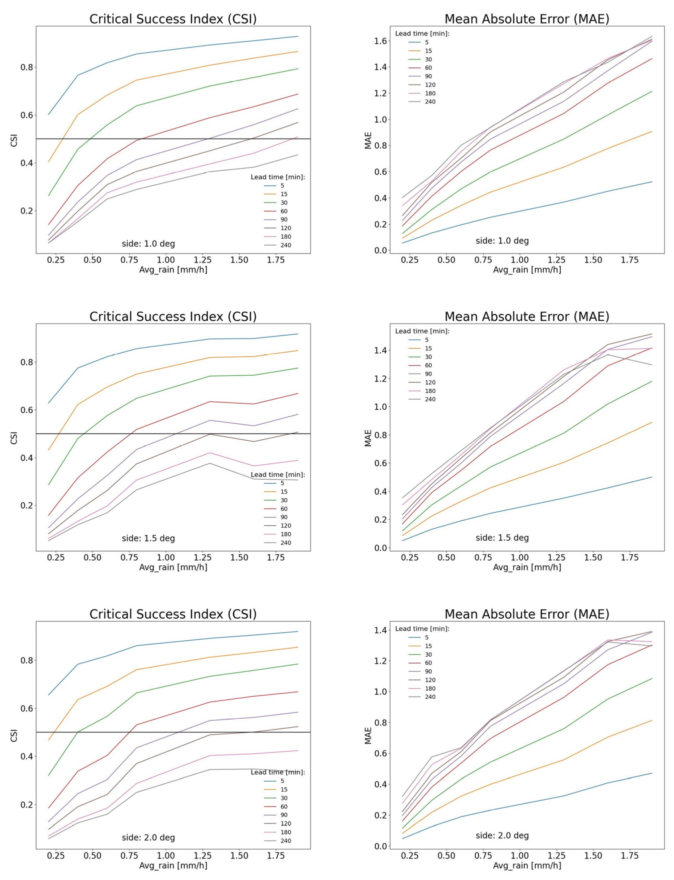
An analysis of nowcasting accuracy relative to the average rain rate for fixed lead times was performed considering all phenomena for the selected period. Figure 8 illustrates how nowcasting accuracy generally increases as the average rain rate increases. Specifically, the minimum average rain rate required to achieve acceptable accuracy increases progressively with lead time. Correspondingly, the MAE thresholds below which nowcasting is considered sufficiently accurate rise with higher rain rates, as relative error decreases. As observed in previous analyses, the accuracy of nowcasting remains largely independent of the selected domain size.

In detail, for a lead time of 5 min, acceptable nowcasting performance is achieved for average rain rates exceeding 0.1 mm/h. For longer lead times, including 15, 30, 60, 90, 120, and 180 min, the corresponding thresholds increase to approximately 0.2, 0.4, 0.8, 1.5, and beyond 2 mm/h, respectively.

Analysing the MAE trends, we observed that these can reasonably be fitted with a straight line with a positive slope coefficient less than 1. This trend indicates that the relative error decreases as the average rain rate increases, as the absolute error approximately increases proportionally to the value of the average rain rate.

Table 2. The fittings of R² of MAE, reported as a function of average rain rate for different domain areas (side measured in degrees) and lead times (in minutes).

Side	Lead Time	Fitting	R2
1	5	y = 0.3x + 0.0	0.99
1	15	y = 0.5x + 0.0	0.99
1	30	y = 0.6x + 0.1	0.99
1	60	y = 0.7x + 0.1	0.99
1	90	y = 0.8x + 0.2	0.98
1	120	y = 0.8x + 0.2	0.98
1	180	y = 0.7x + 0.3	0.97
1.5	5	y = 0.3x + 0.0	0.99
1.5	15	y = 0.5x + 0.0	0.99
1.5	30	y = 0.6x + 0.1	0.99
1.5	60	y = 0.7x + 0.1	0.98
1.5	90	y = 0.8x + 0.2	0.97
1.5	120	y = 0.7x + 0.2	0.95
1.5	180	y = 0.7x + 0.3	0.94
2.0	5	y = 0.2x + 0.0	0.99
2.00	15	y = 0.4x + 0.0	0.99
2.0	30	y = 0.6x + 0.1	0.99
2.0	60	y = 0.7x + 0.1	0.98
2.0	90	y = 0.7x + 0.2	0.97
2.0	120	y = 0.7x + 0.2	0.97
2.0	180	y = 0.6x + 0.3	0.95

reports these fittings in function for the lead time and study domain areas.

Note that the slope of the lines increases with the lead time; this behaviour is simply explained by observing that the difference between measurement and nowcasting values increases as the lead time increases.

3.1.3. Dependence of Nowcasting Accuracy on Rainfall Regimes

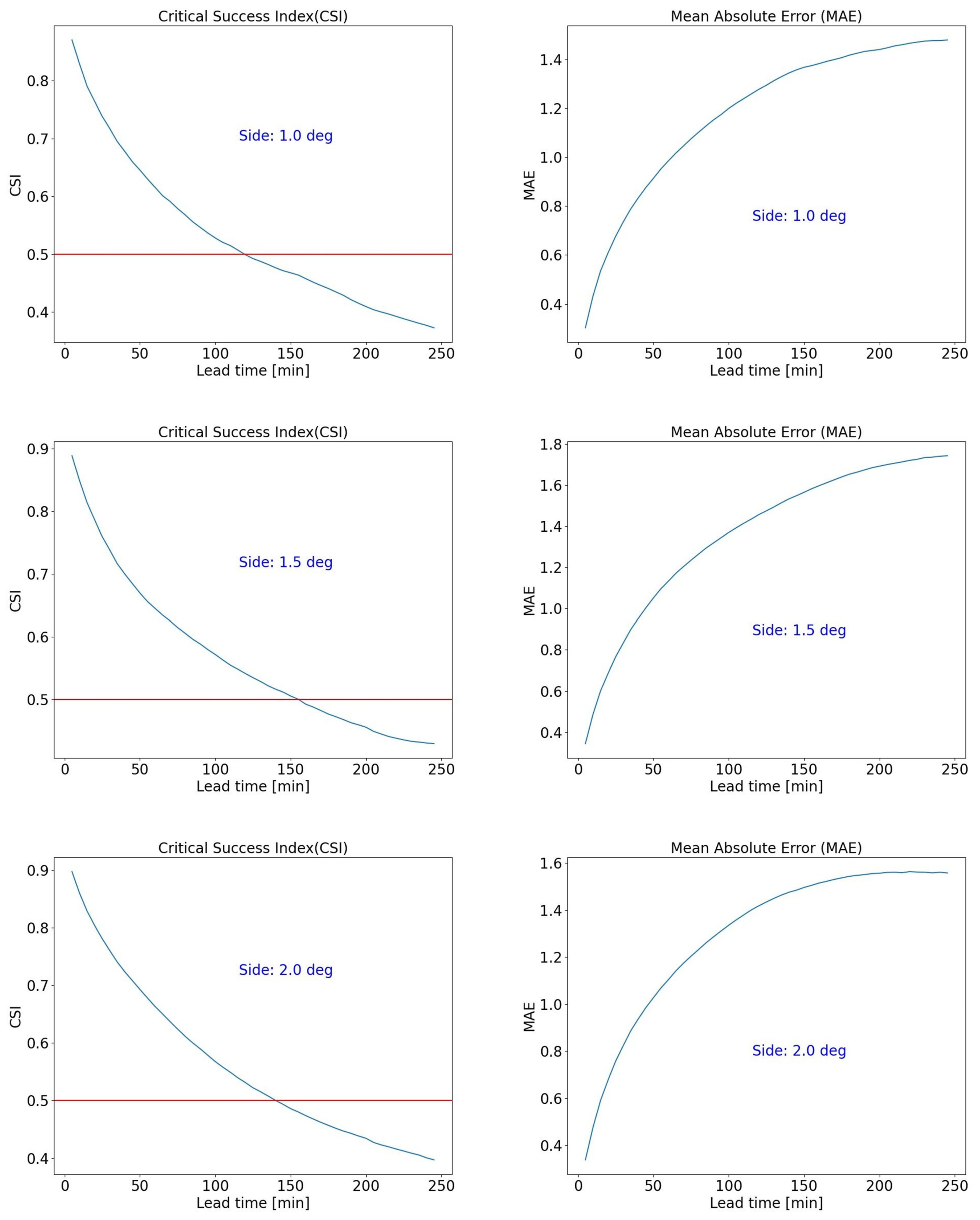
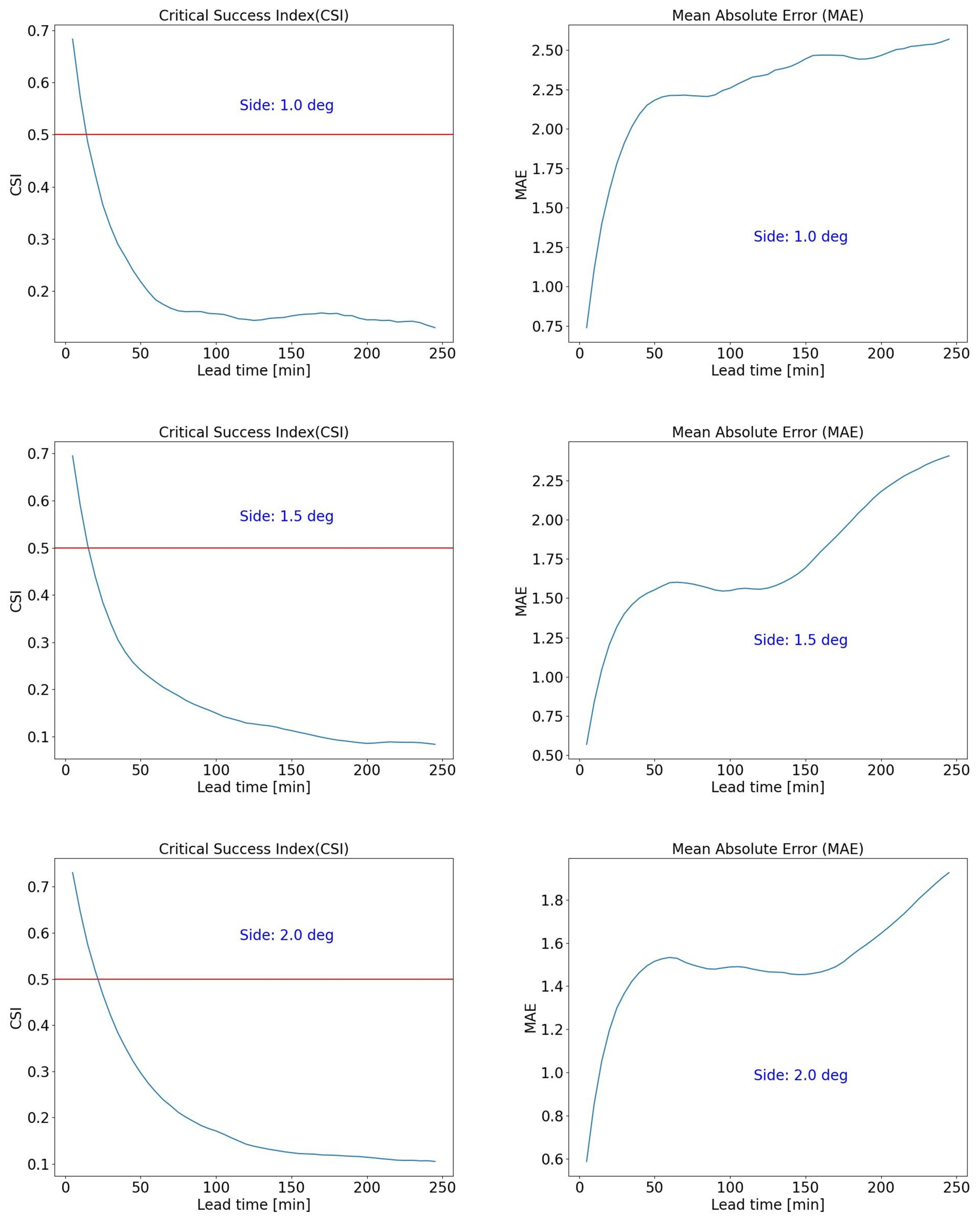
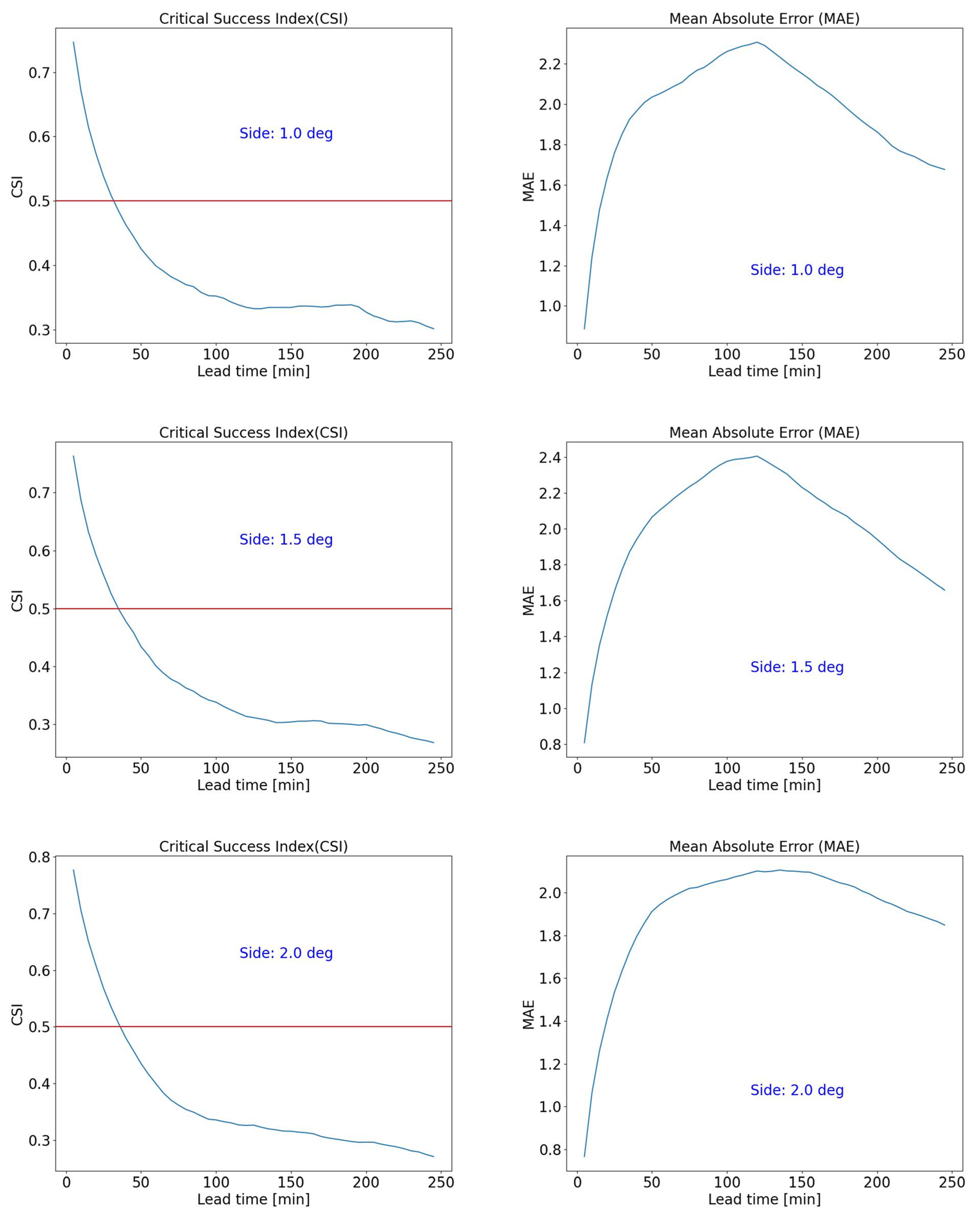
Regarding the analysis of nowcasting accuracy for different rainfall regimes, we examined the dependence of CSI and MAE on the lead time for all average rain rate values of the selected phenomena. The limited availability of measurements precludes a more detailed analysis. Figure 9, Figure 10, Figure 11 and Figure 12 depict the nowcasting analysis for two stratiform and two convective phenomena, respectively. The results reveal a higher nowcasting performance for stratiform phenomena compared to convective ones. The reason for this behaviour can be found in the significant spatio-temporal variability of the latter phenomena and the resulting difficulty in tracking and predicting their evolution. The maximum acceptable lead time for nowcasting exceeds 100 min for stratiform phenomena and is less than 50 min for convective ones. It is noted that the value of the maximum lead time can vary with the area size for stratiform phenomena but remains constant for convective ones. This behaviour is due to the different natures of the phenomena. Stratiform phenomena involve precipitation over wide areas, so considering different domain size can lead to significantly different precipitation patterns. Conversely, convective phenomena, which affect limited areas, result in similar precipitation patterns across all considered areas, if a phenomenon persists over all different areas.

4. Discussion

This study validates a computationally efficient nowcasting methodology that offers a robust compromise between forecast accuracy and low resource demands. The method is particularly well suited for operational deployment in meteorological centres with limited computational capacity, providing timely and actionable short-term precipitation forecasts to support weather alert systems and emergency preparedness. The technique was applied to a comprehensive two-year dataset (2022–2023) of radar observations over the Tuscany region, revealing several key insights into the behaviour and performance of the method under real-world operational conditions.

• Dependence on Precipitation Persistence:

As expected, the method performs best when precipitation intensity remains relatively stable throughout the forecast horizon. This assumption of intensity persistence is an inherent feature of the Lagrangian deterministic approach. Stratiform rainfall events, characterised by low variability and high temporal coherence, align well with this assumption and lead to better forecast skill. Conversely, during convective episodes, where rainfall patterns evolve rapidly and irregularly, forecast accuracy deteriorates.

• Relationship Between Intensity and Lead Time:

Quantitative evaluations using the Critical Success Index (CSI) and Mean Absolute Error (MAE) indicate that the method’s performance improves with higher average rain rates and shorter lead times. Specifically, intense precipitation events extend the window of reliable forecast skill, while accuracy declines more rapidly for low-intensity scenarios. Nevertheless, this drop in performance is of limited operational concern, as light rainfall events typically do not require emergency response or alert issuance.

• Robustness Across Spatial Domains:

The nowcasting method demonstrated consistent performance across different spatial scales (from 1° × 1° to 2° × 2°), with no systematic degradation of accuracy observed.

• Operational Relevance:

The overall results confirm the method’s value for real-time applications, particularly for institutions that need a balance between forecasting skill and processing speed. Its simplicity and computational efficiency make it an appealing solution for regional or national alert systems, especially where convective nowcasting remains challenging.

• Comparison with Advanced Methods:

While the method is algorithmically simple, its performance is competitive with more complex forecasting approaches, especially when high-performance hardware is not available. For instance, deep learning-based nowcasting frameworks, such as PredRNN++, RainNet, and other GAN-based models [14,15,16], often require substantial computing power and training data. These models may show better adaptability under convective regimes, but at a cost in terms of reproducibility, transparency, and portability.

• Integration with More Complex Nowcasting Chains:

The method’s modular structure also offers opportunities for integration within more complex nowcasting chains. DenseRotation outputs could serve as deterministic baselines in ensemble probabilistic frameworks or be used to guide adaptive updates in hybrid systems combining radar and NWP data [36]. Future developments will explore such integrations and test the method under varying climatic and orographic conditions to evaluate its generalisability.

5. Conclusions

While this study does not introduce novel algorithms or theoretical advancements, its contribution lies in the comprehensive validation of an existing deterministic nowcasting approach over a large and diverse operational dataset. To the best of our knowledge, this is the first time the DenseRotation nowcasting scheme has been systematically tested using a two-year radar dataset from Tuscany, a region with varied precipitation dynamics and complex terrain.

The analysis covered a broad range of precipitation regimes, including both stratiform and convective events, and multiple spatial domains. This experimental setup was designed specifically to support the LaMMA Consortium, the official regional meteorological service, in enhancing its capability for timely and reliable weather alert issuance. The findings confirm that the proposed method

• Performs reliably under stratiform and high-intensity precipitation conditions.
• Maintains sufficient accuracy for lead times up to 2 h in favourable conditions.
• Is computationally lightweight and suitable for real-time operations on standard hardware.
• Is modular and scalable to other geographic regions and radar configurations.

It is important to acknowledge that the results are region-specific and may vary in different climatic or orographic contexts. Nonetheless, the methodology’s general structure is adaptable and can be transferred to other settings with minimal adjustments.

The nowcasting procedure is currently undergoing final testing. Preliminary results are encouraging, showing promise in both forecast skill and timeliness. In the near future, the method will be operationally deployed at the LaMMA Consortium, where it will be integrated into daily workflows and continuously validated against radar data and other observational sources. This work contributes to the broader goal of making effective and efficient nowcasting tools more accessible, particularly in regions where real-time forecasting must be achieved with modest computational infrastructure.

Future developments will aim at incorporating hybrid frameworks, where DenseRotation can be used to initialise or guide probabilistic or machine learning systems (e.g., ensemble NWP models [36] or CNN-based classifiers [16]), thereby enhancing its applicability even under convective conditions.

In summary, this work demonstrates that an efficient, transparent, and easily deployable radar nowcasting approach can meet key operational requirements. It bridges the gap between methodological simplicity and practical readiness, providing a scalable solution for real-time applications in meteorology and civil protection.

References

- Biondi, A.; Facheris, L.; Argenti, F.; Cuccoli, F.; Antonini, A.; Melani, S. Assessing Quantitative Precipitation Estimation Methods Based on the Fusion of Weather Radar and Rain-Gauge Data. IEEE Geosci. Remote Sens. Lett. 2024, 21, 3508005. [Google Scholar] [CrossRef]
- Antonini, A.; Melani, S.; Corongiu, M.; Romanelli, S.; Mazza, A.; Ortolani, A.; Gozzini, B. On the implementation of a regional X-band weather radar network. Atmosphere 2017, 8, 25. [Google Scholar] [CrossRef]
- Mazza, A.; Antonini, A.; Melani, S.; Ortolani, A. Re-calibration of cumulative rainfall estimates by weather radar over a large area. J. Appl. Remote Sens. 2015, 9, 095993. [Google Scholar] [CrossRef]
- Antonini, A.; Melani, S.; Ortolani, A.; Pieri, M.; Gozzini, B. Qualitative weather radar mosaic in a multi-sensor rainfall monitoring approach. J. Appl. Remote Sens. 2012, 6, 063572. [Google Scholar] [CrossRef]
- Scognamiglio, G.; Rucci, A.; Vaccaro, A.; Adirosi, E.; Sapienza, F.; Giannetti, F.; Bacci, G.; Angeloni, S.; Baldini, L.; Roversi, G.; et al. Deep Learning for Opportunistic Rain Estimation via Satellite Microwave Links. Sensors 2024, 24, 6944. [Google Scholar] [CrossRef] [PubMed]
- Angeloni, S.; Adirosi, E.; Sapienza, F.; Giannetti, F.; Francini, F.; Magherini, L.; Valgimigli, A.; Vaccaro, A.; Melani, S.; Antonini, A.; et al. Enhanced Estimation of Rainfall From Opportunistic Microwave Satellite Signals. IEEE Trans. Geosci. Remote Sens. 2024, 62, 4101312. [Google Scholar] [CrossRef]
- Sapienza, F.; Bacci, G.; Giannetti, F.; Lottici, V.; Vaccaro, A.; Serafino, G.; Ortolani, A.; Caparrini, F.; Antonini, A.; Melani, S.; et al. A Feasibility Study on Opportunistic Rainfall Measurement From Satellite TV Broadcasts. URSI Radio Sci. Lett. 2023, 4, 2022. [Google Scholar] [CrossRef]
- Ortolani, A.; Caparrini, F.; Melani, S.; Baldini, L.; Giannetti, F. An EnKF-Based Method to Produce Rainfall Maps from Simulated Satellite-to-Ground MW-Link Signal Attenuation. J. Hydrometeorol. 2021, 22, 1333–1350. [Google Scholar] [CrossRef] [PubMed]
- Giannetti, F.; Reggiannini, R.; Moretti, M.; Adirosi, E.; Baldini, L.; Facheris, L.; Antonini, A.; Melani, S.; Bacci, G.; Petrolino, A.; et al. Real-Time Rain Rate Evaluation via Satellite Downlink Signal Attenuation Measurement. Sensors 2017, 17, 1864. [Google Scholar] [CrossRef] [PubMed]
- Pudashine, J.; Guyot, A.; Petitjean, F.; Pauwels, V.R.; Uijlenhoet, R.; Seed, A.; Prakash, M.; Walker, J.P. Deep learning for an improved prediction of rainfall retrievals from commercial microwave links. Water Resour. Res. 2020, 56, 2019–026255. [Google Scholar] [CrossRef]
- Sohail Afzal, M.; Shah, S.H.H.; Cheema, M.J.M.; Ahmad, R. Real time rainfall estimation using microwave signals of cellular communication networks: A case study of faisalabad, pakistan. Hydrol. Earth Syst. Sci. Discuss. 2018. [Google Scholar] [CrossRef]
- Roversi, G.; Alberoni, P.P.; Fornasiero, A.; Porcù, F. Commercial microwave links as a tool for operational rainfall monitoring in Northern Italy. Atmos. Meas. Tech. 2020, 13, 5779–5797. [Google Scholar] [CrossRef]
- Overeem, A.; Leijnse, H.; Uijlenhoet, R. Measuring urban rainfall using microwave links from commercial cellular communication networks. Water Resour. Res. 2011, 47, W12505. [Google Scholar] [CrossRef]
- Ha, J.H.; Lee, H. Enhancing Rainfall Nowcasting Using Generative Deep Learning Model with Multi-Temporal Optical Flow. Remote Sens. 2023, 15, 5169. [Google Scholar] [CrossRef]
- Tuyen, D.N.; Tuan, T.H.; Le, X.H.; Tunh, N.T.; Chau, T.K.; Hai, P.V.; Gerogiannis, V.C.; Son, L.H. RainPredRNN: A New Approach for Precipitation Nowcasting with Weather Radar Echo Images Based on Deep Learning. Axioms 2022, 11, 107. [Google Scholar] [CrossRef]
- Ayzel, G.; Heistermann, M.; Sorokin, A.; Nikitin, O.; Lukyanova, O. All convolutional neural networks for radar-based precipitation nowcasting. Procedia Comput. Sci. 2019, 150, 186–192. [Google Scholar] [CrossRef]
- Ayzel, G.; Heistermann, M.; Winterrath, T. Optical flow models as an open benchmark for radar-based precipitation nowcasting (rainymotion v0.1). Geosci. Model Dev. 2019, 12, 1387–1402. [Google Scholar] [CrossRef]
- Pulkkinen, S.V.; Chandrasekar, V.; Harri, A.M. Fully Spectral Method for Radar-Based Precipitation Nowcasting. IEEE J. Sel. Top. Appl. Earth Obs. Remote Sens. 2019, 12, 1369–1382. [Google Scholar] [CrossRef]
- Bechini, R.; Chandrasekar, V. An Enhanced Optical Flow Technique for Radar Nowcasting of Precipitation and Winds. J. Atmos. Ocean. Technol. 2017, 34, 2637–2658. [Google Scholar] [CrossRef]
- Bowler, E.H.; Pierce, C.E.; Seed, A. Development of a precipitation nowcasting algorithm based upon optical flow techniques. J. Hydrol. 2004, 288, 74–91. [Google Scholar] [CrossRef]
- Pulkkinen, S.; Nerini, D.; Perez Hortal, A.A.; Velasco-Forero, C.; Seed, A.; Germann, U.; Foresti, L. Pysteps: An open-source Python library for probabilistic precipitation nowcasting (v1.0). Geosci. Model Dev. 2019, 12, 4185–4219. [Google Scholar] [CrossRef]
- Seed, A.W.; Pierce, C.E.; Norman, K. Formulation and evaluation of a scale decomposition-based stochastic precipitation nowcast scheme. Water Resour. Res. 2013, 49, 6624–6641. [Google Scholar] [CrossRef]
- Shi, X.; Lee, Y.H.; Ha, J.-C.; Chang, D.-E.; Bellon, A.; Zawadzki, I.; Lee, G. McGill Algorithm for Precipitation Nowcasting by Lagrangian Extrapolation (MAPLE) Applied to the South Korean Radar Network. Part II: Real-Time Verification for the Summer Season. Asia-Pac. J. Atmos. Sci. 2010, 46, 383–391. [Google Scholar]
- Germann, U.; Zawadzki, I. Scale-Dependence of the Predictability of Precipitation from Continental Radar Images. Part I: Description of the Methodology. Mon. Weather. Rev. 2002, 130, 2859–2873. [Google Scholar] [CrossRef]
- Woo, W.C.; Wong, W.K. Operational Application of Optical Flow Techniques to Radar-Based Rainfall Nowcasting. Atmosphere 2017, 8, 48. [Google Scholar] [CrossRef]
- Austin, G.L.; Bellon, A. The use of digital weather radar records for short-term precipitation forecasting. Q. J. R. Meteorol. Soc. 1974, 100, 658–664. [Google Scholar] [CrossRef]
- Kroeger, T.; Timofte, R.; Dai, D.; Van Gool, L. Fast optical flow using dense inverse search. In Computer Vision—ECCV 2016; Lecture Notes in Computer Science Series; Leibe, B., Matas, J., Sebe, N., Welling, M., Eds.; Springer: Berlin/Heidelberg, Germany, 2016; Volume 9908, pp. 471–488. [Google Scholar]
- Guo, Y.; Shao, C.; Su, A. Comparative Evaluation of Rainfall Forecasts during the Summer of 2020 over Central East China. Atmosphere 2023, 14, 992. [Google Scholar] [CrossRef]
- Jolliffe, I.T.; Stephenson, D.B. (Eds.) Forecast Verification: A Practitioner’s Guide in Atmospheric Science; John Wiley & Sons: Hoboken, NJ, USA, 2012. [Google Scholar]
- Bowler, N.E.; Pierce, C.E.; Seed, A.W. STEPS: A probabilistic precipitation forecasting scheme which merges an extrapolation nowcast with downscaled NWP. Q. J. R. Meteorol. Soc. 2006, 132, 2127–2155. [Google Scholar] [CrossRef]
- Foresti, L.; Reyniers, M.; Seed, A.; Delobbe, L. Development and verification of a real-time stochastic precipitation nowcasting system for urban hydrology in Belgium. Hydrol. Earth Syst. Sci. 2016, 20, 505–527. [Google Scholar] [CrossRef]
- Dipartimento Della Protezione Civile. Piattaforma Radar. Available online: https://mappe.protezionecivile.gov.it/it/mappe-rischi/piattaforma-radar/ (accessed on 1 July 2024).
- Dipartimento Della Protezione Civile. Piattaforma Radar. Available online: https://dpc-radar.readthedocs.io/it/latest/clientwss.html (accessed on 1 July 2024).
- Stein, J. Another look at the contingency tables: Scores based on Manhattan distances in the phase space. Meteorol. Appl. 2011, 18, 28–39. [Google Scholar] [CrossRef]
- Hewson, T. The concept of ‘Deterministic limit’. In Proceedings of the 3rd International Verification Methods Workshop, Reading, UK, 31 January–2 February 2007. [Google Scholar]
- Wilson, J.; Megenhardt, D.; Pinto, J. NWP and Radar Extrapolation: Comparisons and Explanation of Errors. Mon. Weather. Rev. 2020, 148, 4783–4798. [Google Scholar] [CrossRef]
Figure 1.
Flowchart of DenseRotation scheme.
Figure 2.
Coverage of Italian territory by the Civil Protection Department radar network.
Figure 3.
The area where the precipitation nowcasting procedure was applied.
Figure 4.
(a) Distribution of the durations [hours] of the analysed phenomena. (b–d) The maximum Average_RR as a function of the phenomena duration for different domain sizes.
Figure 5.
An example of precipitation nowcasting with significant rain rate variation during the analysed periods. Top: radar rainfall estimates and their corresponding nowcasting; bottom: trends of CSI and MAE, and the average rain rate. Note the rapid worsening of the statistical scores over time due to the violation of the quasi-persistence assumption.
Figure 6.
An example of precipitation nowcasting with very limited rain rate variation during the analysed periods (except for the last period, about 20 min.). Top: radar rainfall estimates and their corresponding nowcasting; bottom: trends of
CSI and
MAE and the average rain rate. Note the much less severe worsening of the statistical scores over time with respect to the case of
Figure 5, due to the higher validity of the quasi-persistence assumption.
Figure 7.
CSI (left) and MAE (right column) are shown as functions of the lead time for different ranges of average precipitation. The 0.5 CSI threshold is indicated. From top to bottom, the increasing side of the considered domain area is also indicated (1.0°, 1.5°, 2.0°).
Figure 8.
CSI (left column) and MAE (right column) as functions of average rain rate for different lead times. The 0.5 CSI threshold is indicated. From top to bottom, the pictures refer to the increasing side for the selected domain area, as indicated (1.0°, 1.5°, 2.0°).
Figure 9.
CSI (left column) and MAE (right column) as functions of lead time for a stratiform case study, 5 January 2022 11:00–6 January 2022 02:00. The 0.5 CSI threshold is indicated. From top to bottom, the increasing side of the selected domain area is also indicated (1.0°, 1.5°, 2.0°).
Figure 10.
The same as
Figure 8, but for the stratiform case study extending from 19 March 2023 14:00 UTC to 20 March 2023 08:00 UTC.
Figure 11.
Figure 8, but for the convective case study extending from 18 August 2022 06:00 UTC to 19 August 2022 05:00 UTC.
Figure 12.
Figure 8, but for the convective case study extending from 2 November 2023 13:30 UTC to 3 November 2023 06:00 UTC.