
Meteorological Drivers and Agricultural Drought Diagnosis Based on Surface Information and Precipitation from Satellite Observations in Nusa Tenggara Islands, Indonesia

 , , ,
, , ,  and
and 
Abstract

1. Introduction
2. Materials and Methods
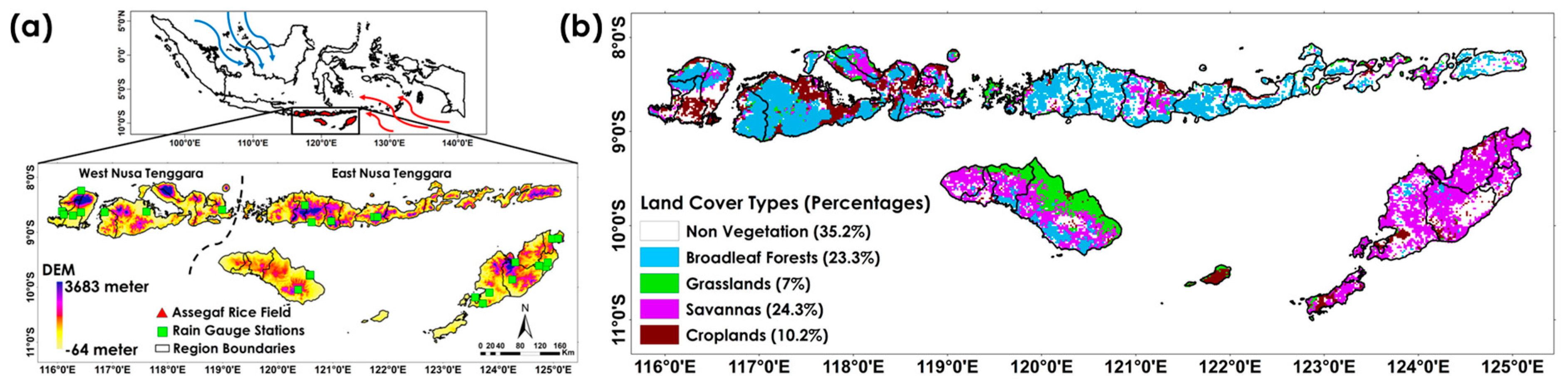
2.1. Study Area
2.2. Data
2.2.1. Himawari-8 AHI Data
2.2.2. Rain Gauge
2.2.3. MODIS Data
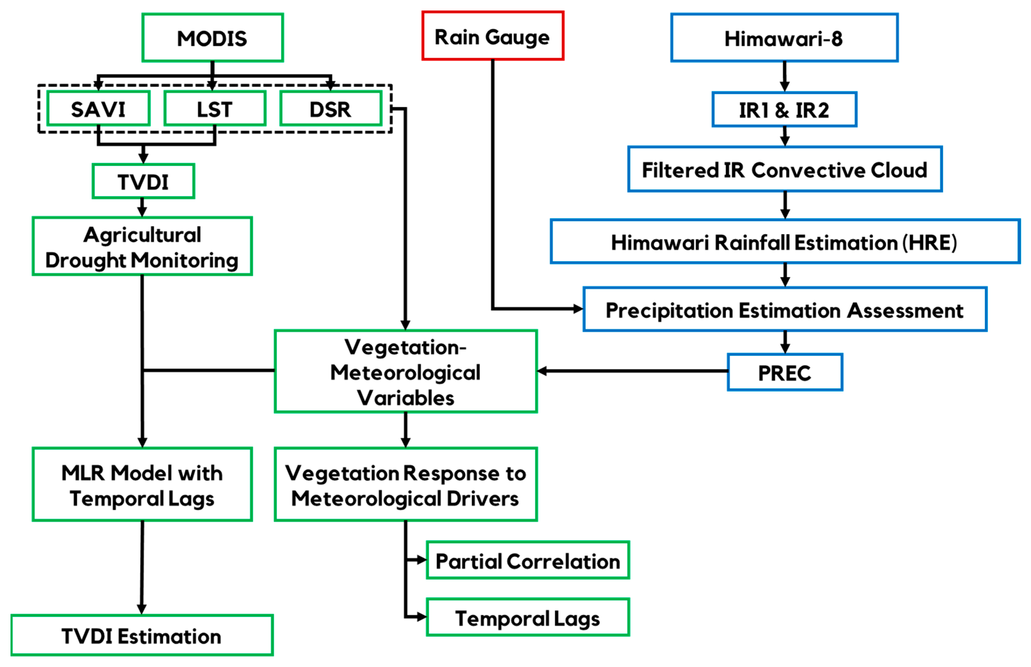
2.3. Methodology
2.3.1. Himawari Rainfall Estimation (HRE)
2.3.2. Calculation of the NDVI and SAVI
2.3.3. Vegetation Anomaly
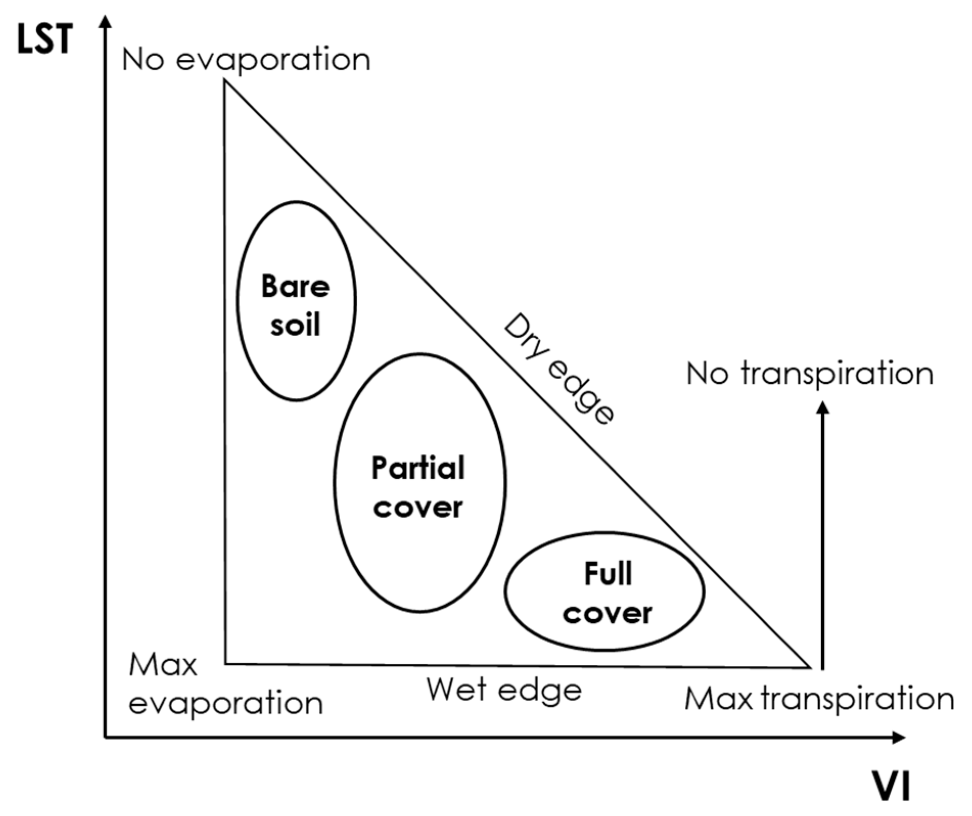
2.3.4. Calculation of the TVDI
2.3.5. Standardized Precipitation Index (SPI)
2.3.6. A Second-Order Partial Correlation
2.3.7. Linear Regression
2.3.8. Multiple Linear Regression (MLR)
2.3.9. Validation Metrics
3. Results
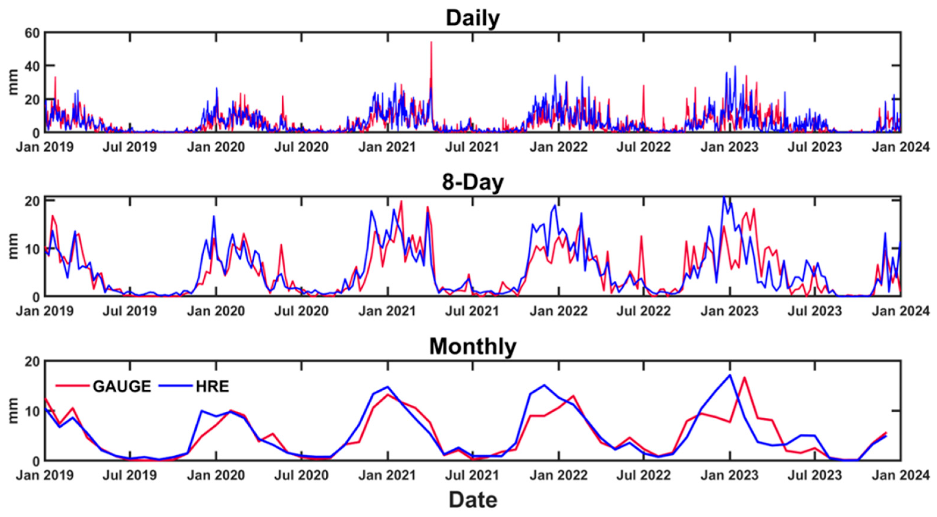
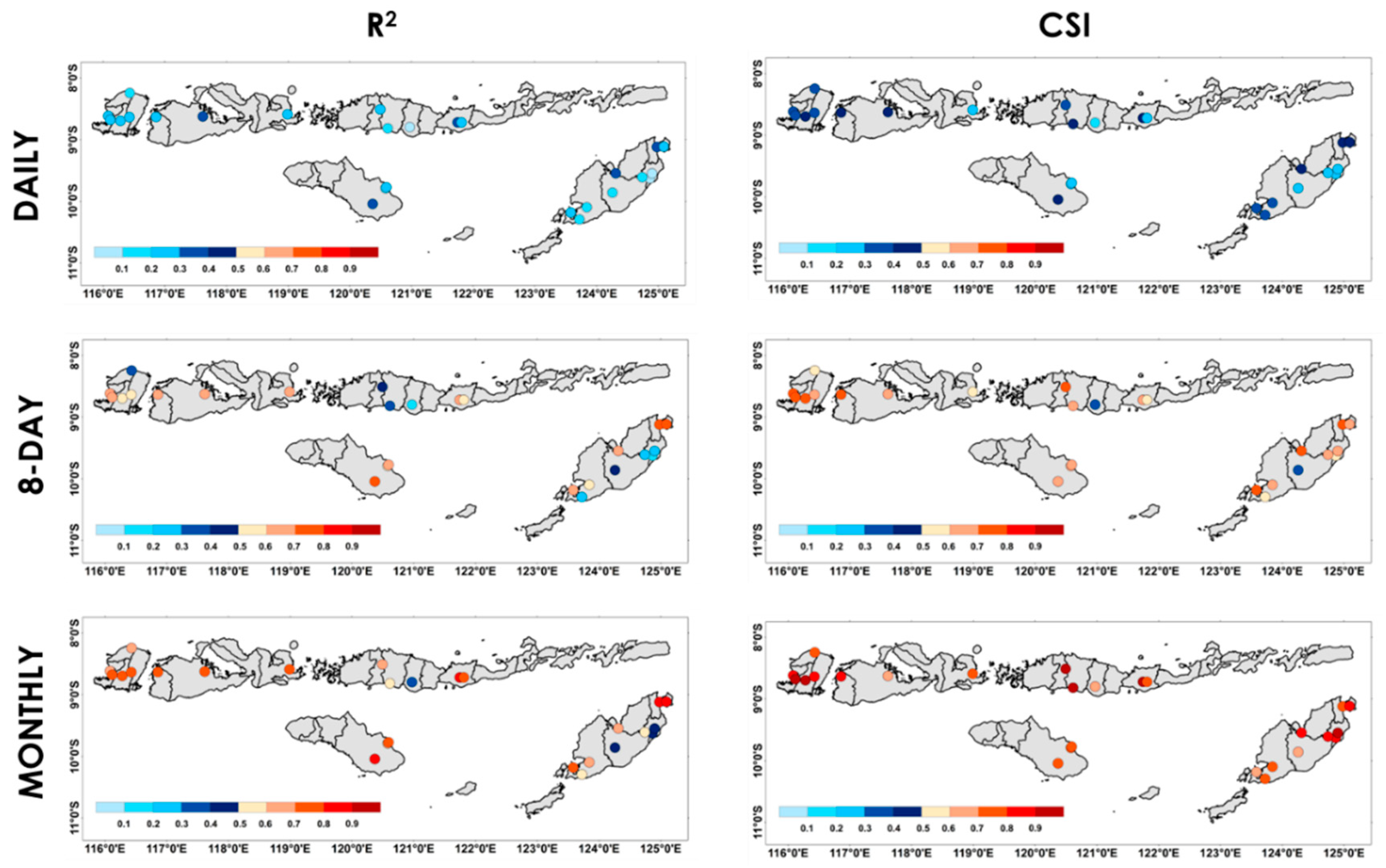
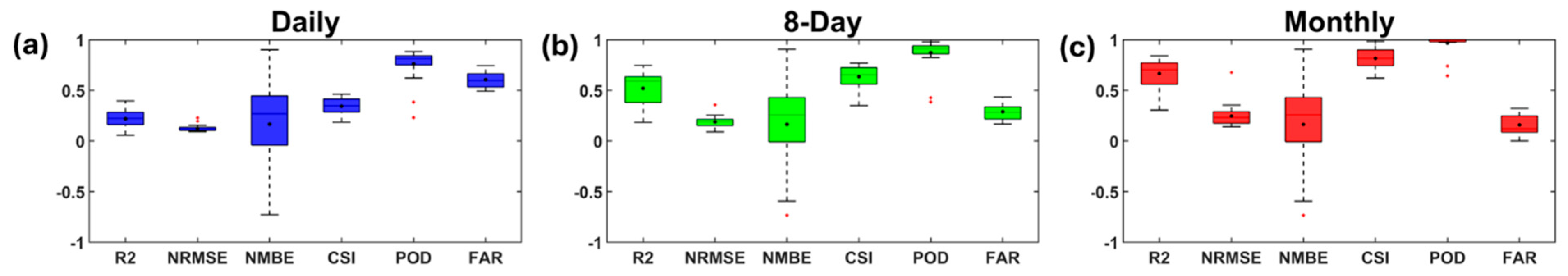
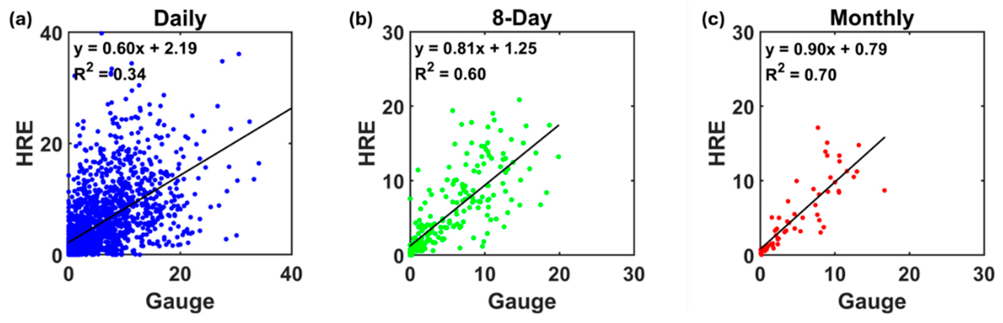
3.1. Reliability Assessment of Himawari-8 Rainfall Estimation (HRE)
3.2. Agricultural Drought and Its Impact on Vegetation
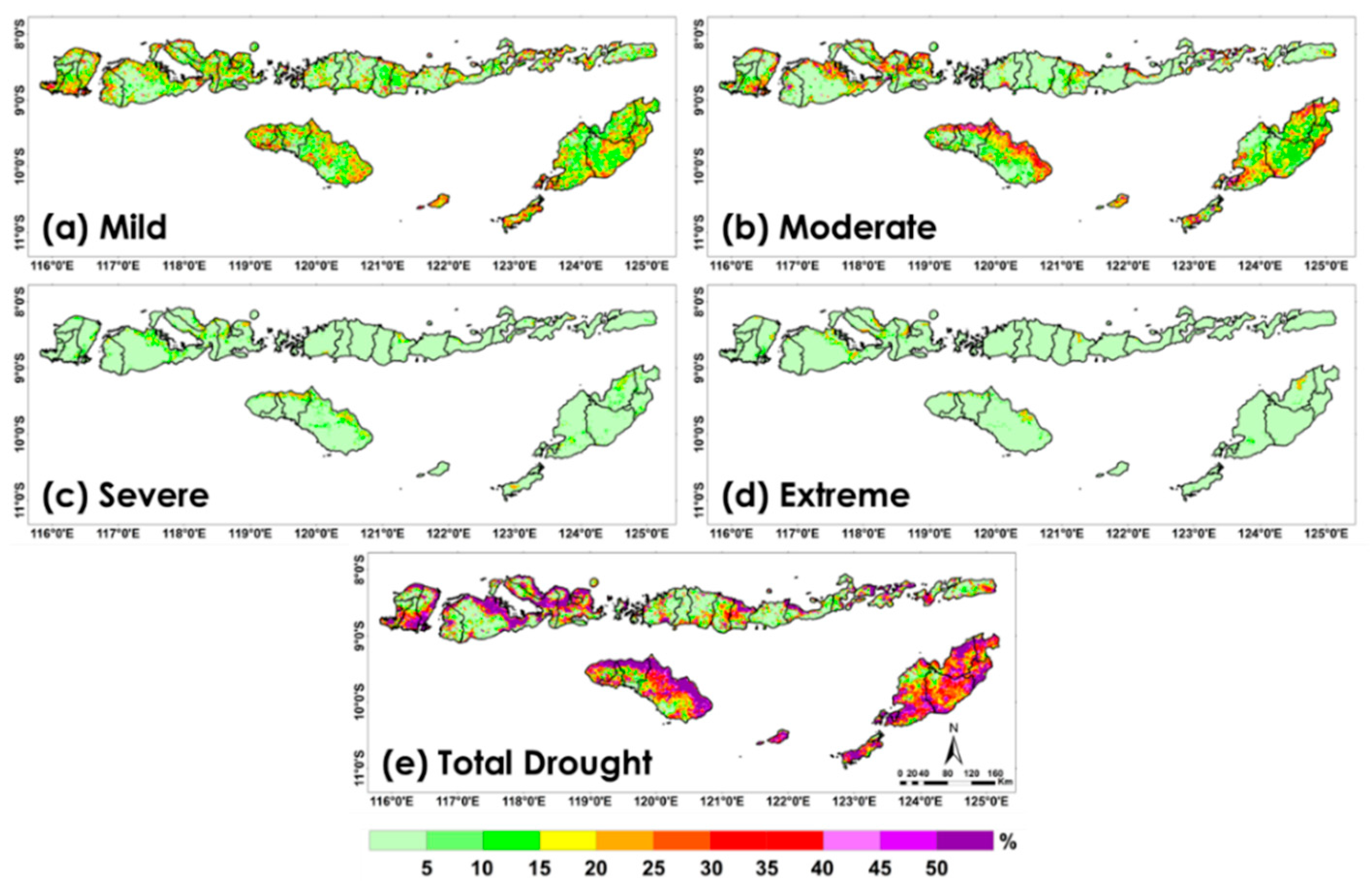
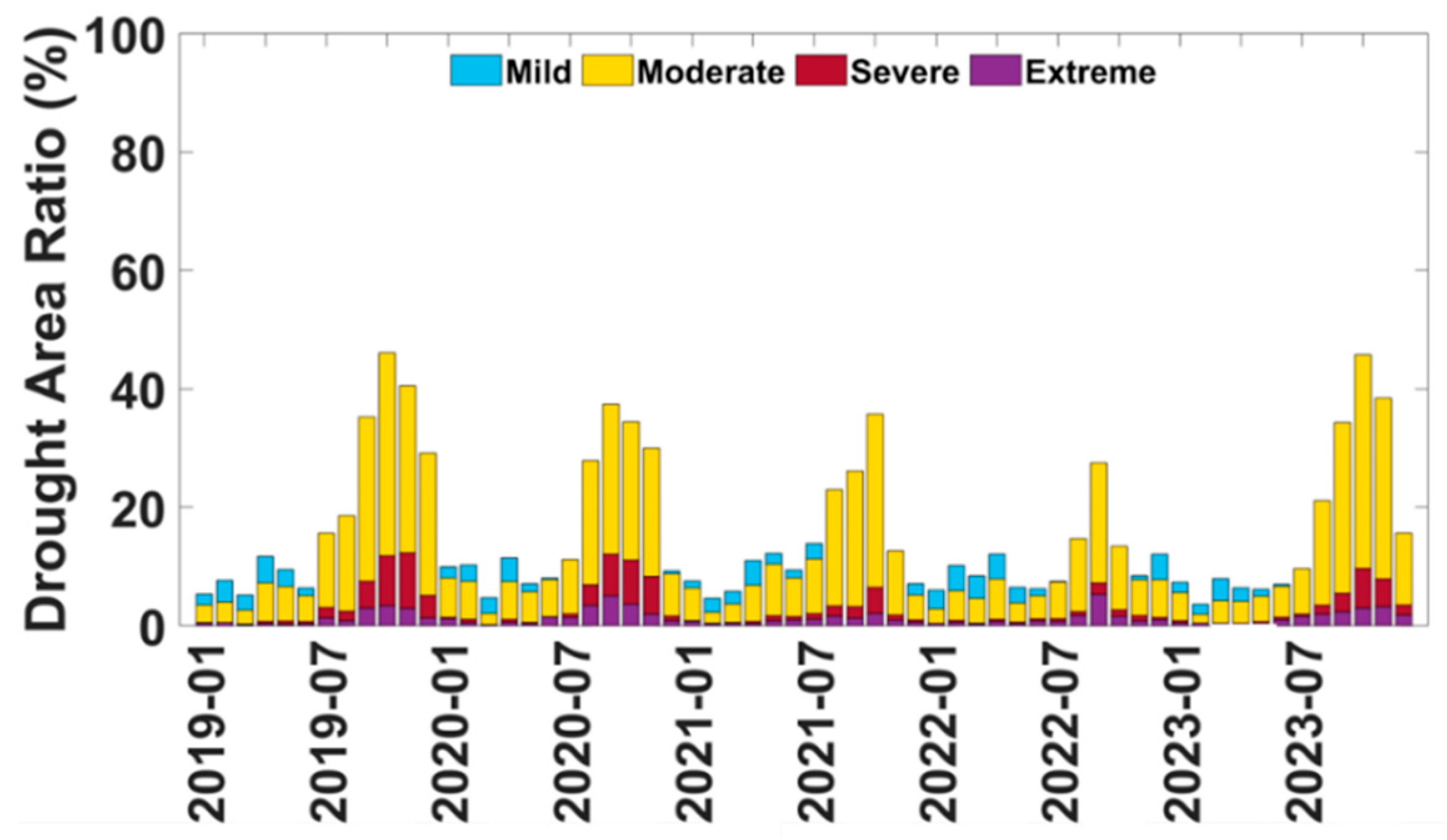
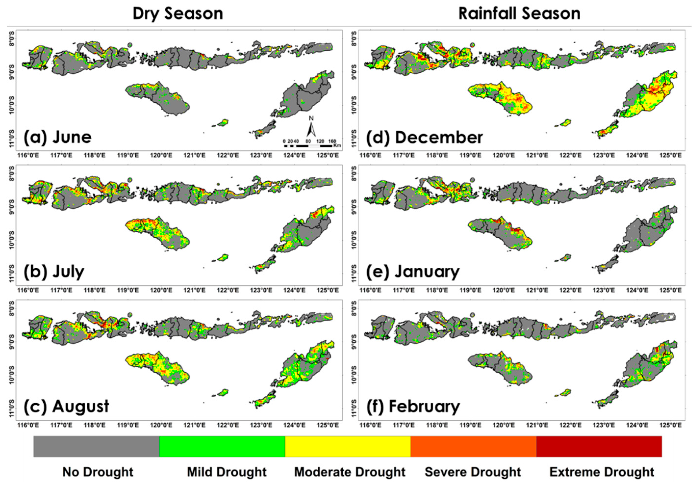
3.2.1. Spatiotemporal Patterns and Agricultural Drought Frequency in NTI
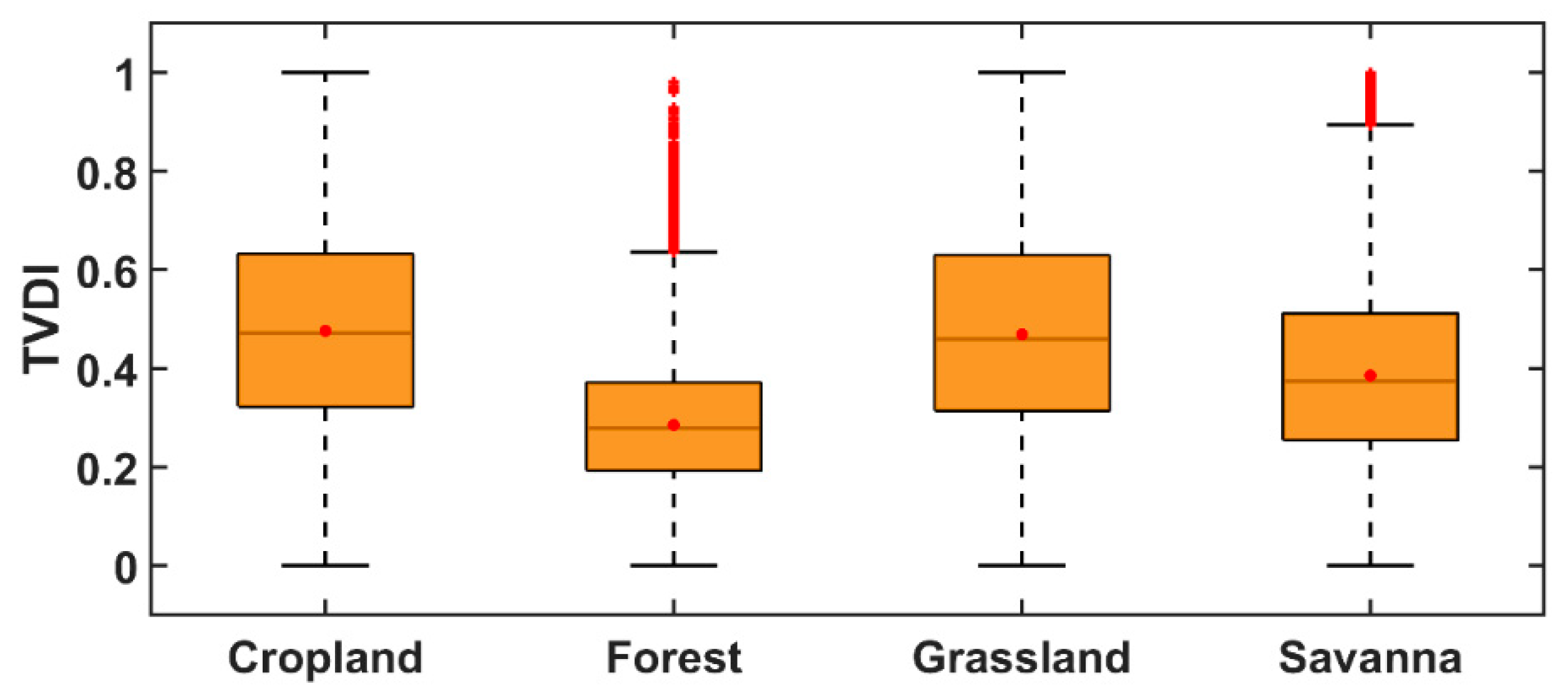
3.2.2. TVDI Variation Across Different Vegetation Types
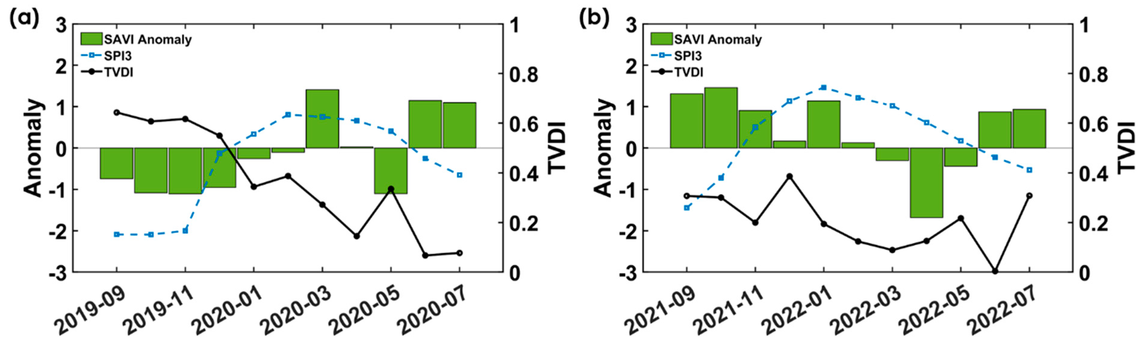
3.2.3. Impact of Agricultural Drought on Rice Crops
3.3. The Relationship Between Meteorological Factors and Both Vegetation and Agricultural Drought
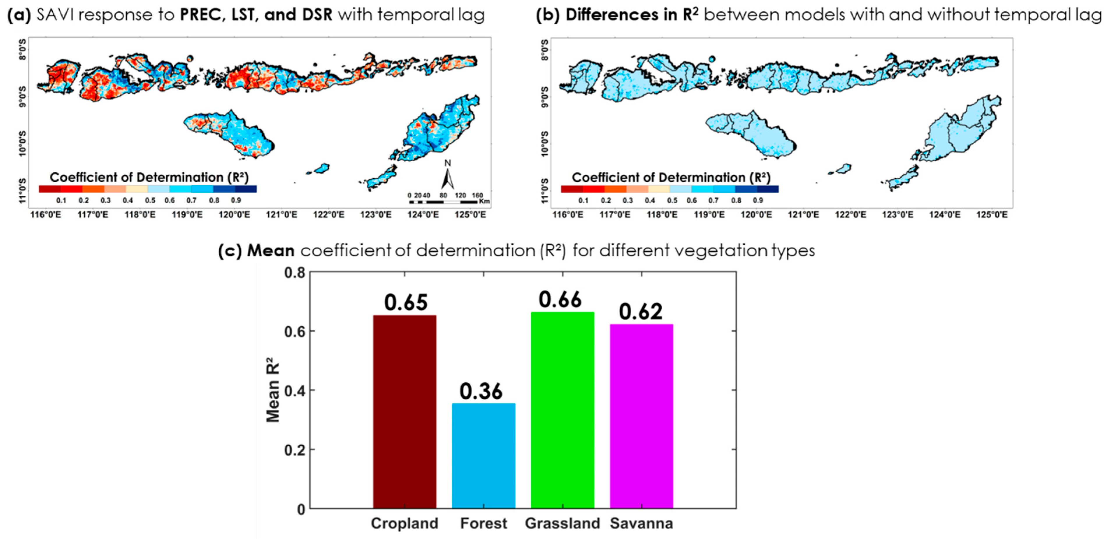
3.3.1. Vegetation Response to Meteorological Factors
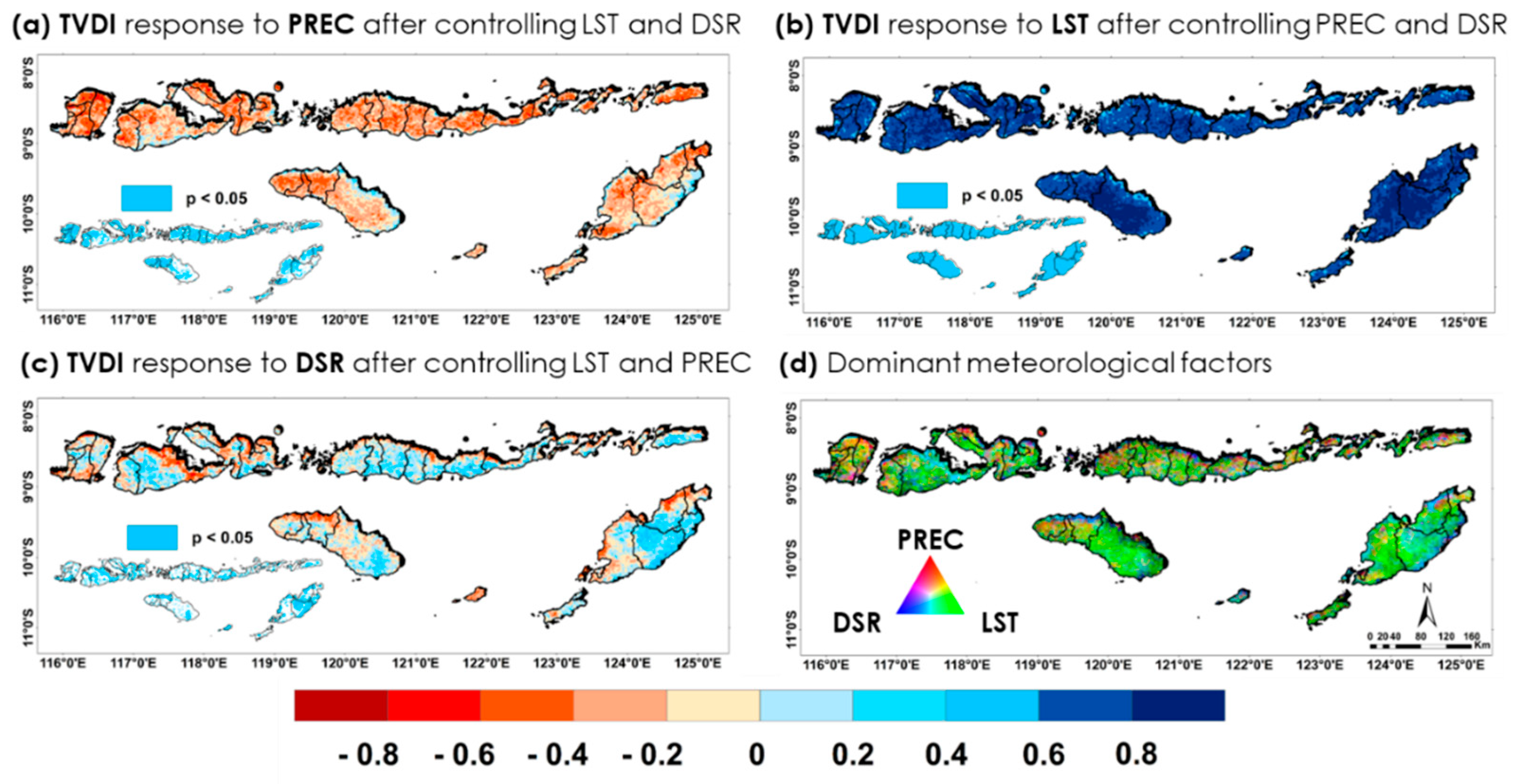
3.3.2. Agricultural Drought Response to Meteorological Factors
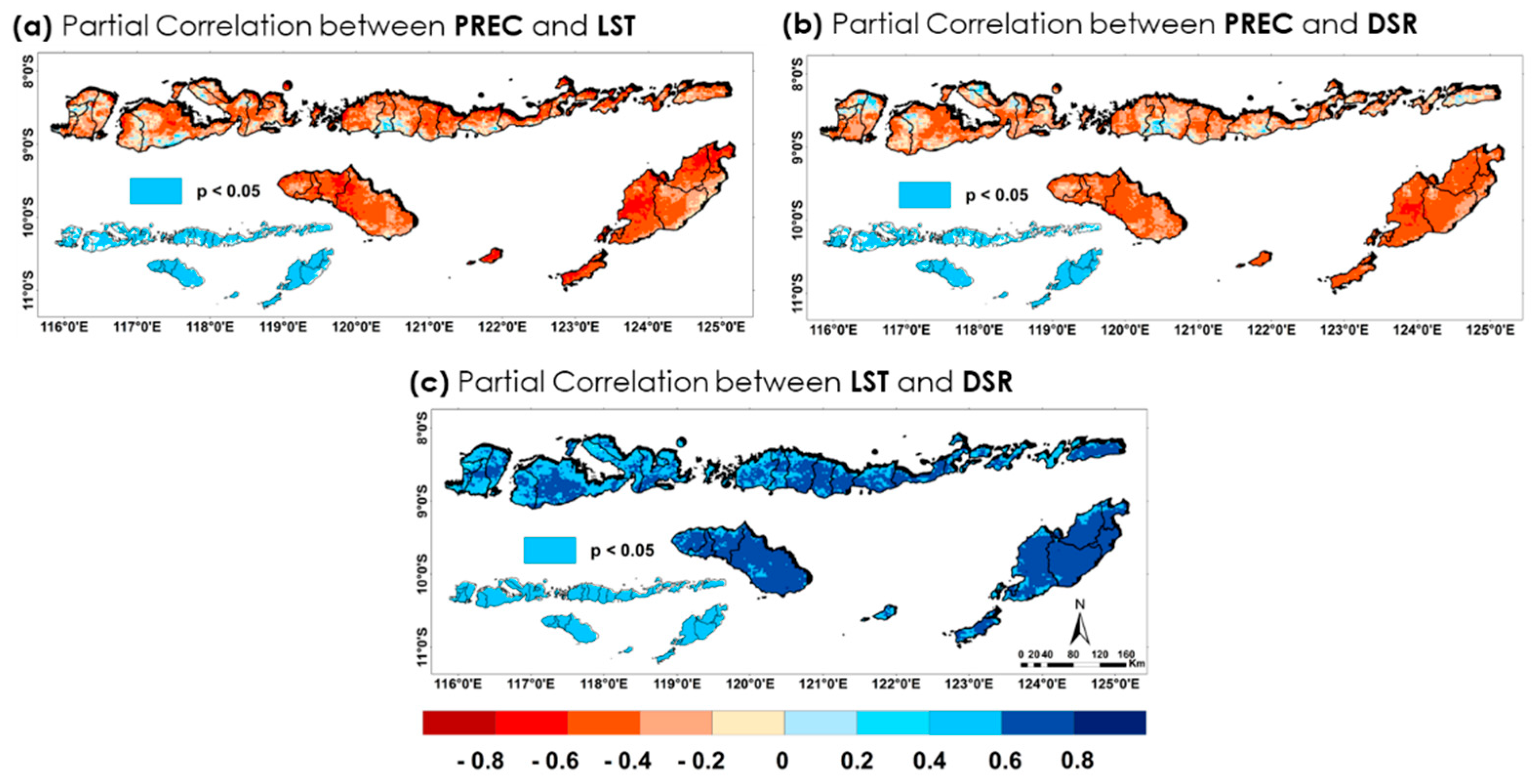
3.3.3. Relationship Between Meteorological Variables
3.4. Agricultural Drought Prediction
4. Discussion
5. Conclusions
- (1)
- A comparative analysis of Himawari-8 rainfall estimation (HRE) data and gauge observations over the NTIs shows that HRE is valuable for regional rainfall monitoring, especially for agricultural drought-related applications. Although daily scale data are affected by short-term disturbances and retrieval limitations, aggregation to 8-day and monthly scales significantly improves the reliability of rainfall estimates. The improved accuracy of continuous and categorical assessment at these timescales supports their application in drought monitoring. Therefore, this study uses HRE at 8-day and monthly intervals as a suitable satellite-based rainfall source to assess and predict agricultural drought dynamics in the NTIs.
- (2)
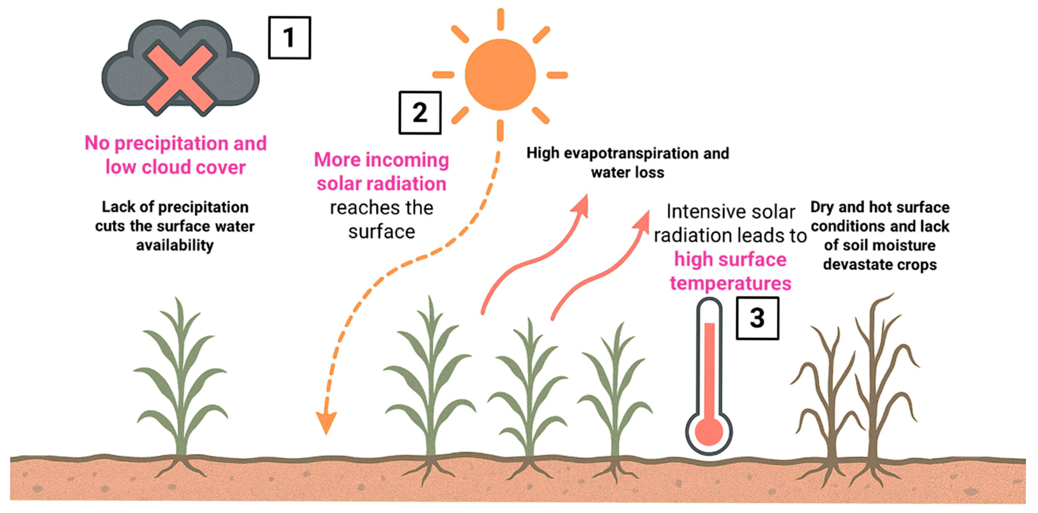
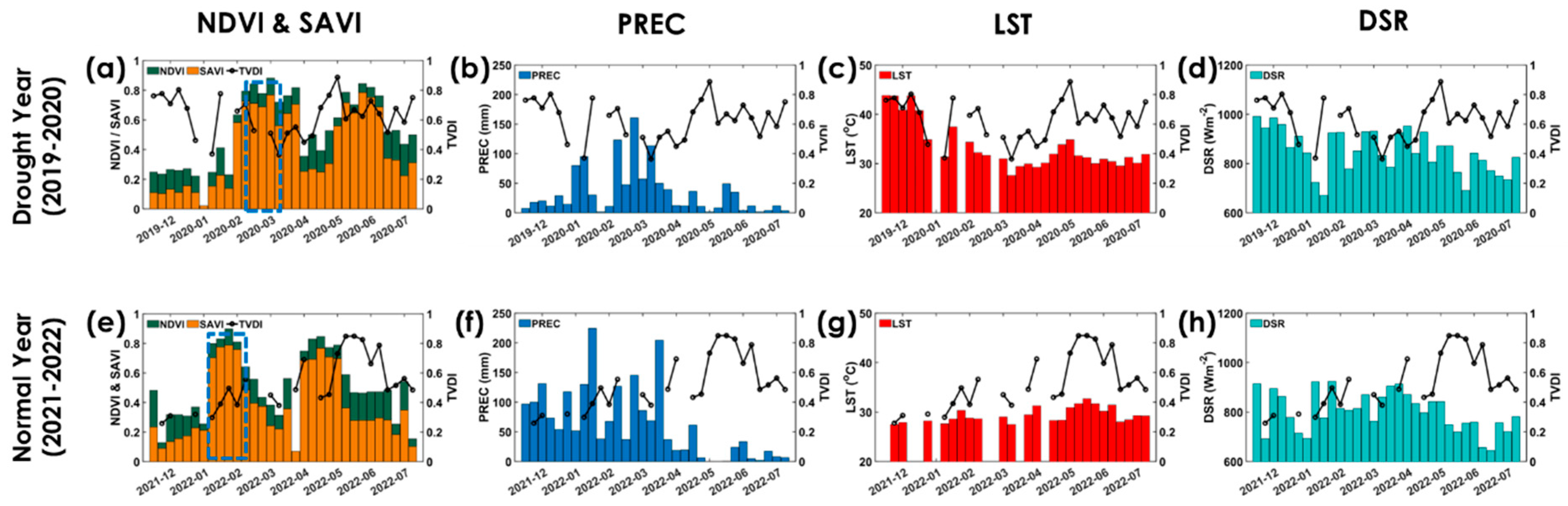
- Agricultural drought in the NTIs is frequent; droughts are generally categorized as being mild to moderate in intensity. In terms of vegetation type, cropland is the most vulnerable to drought, followed by grassland and savannah. In contrast, forest areas show resilience to the impacts of drought. Meteorological factors, such as insufficient rainfall, increased land surface temperature, and radiation, indicate the severity of the drought, as evidenced by the 2019–2020 drought case study. These extreme conditions not only increased the TVDI but also disrupted the cropping cycle of rice, leading to a negative vegetation anomaly due to delays in planting and harvesting.
- (3)
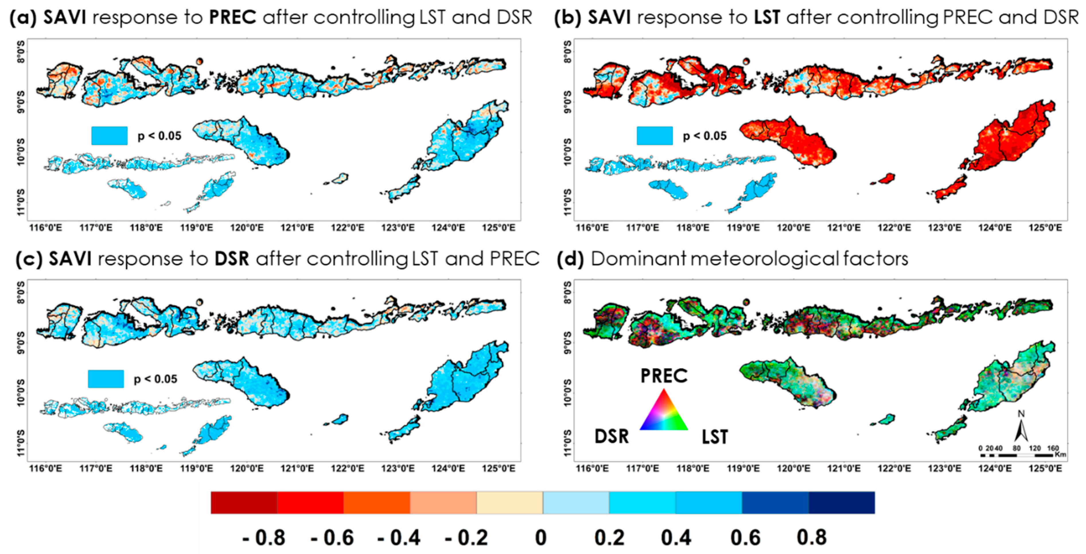
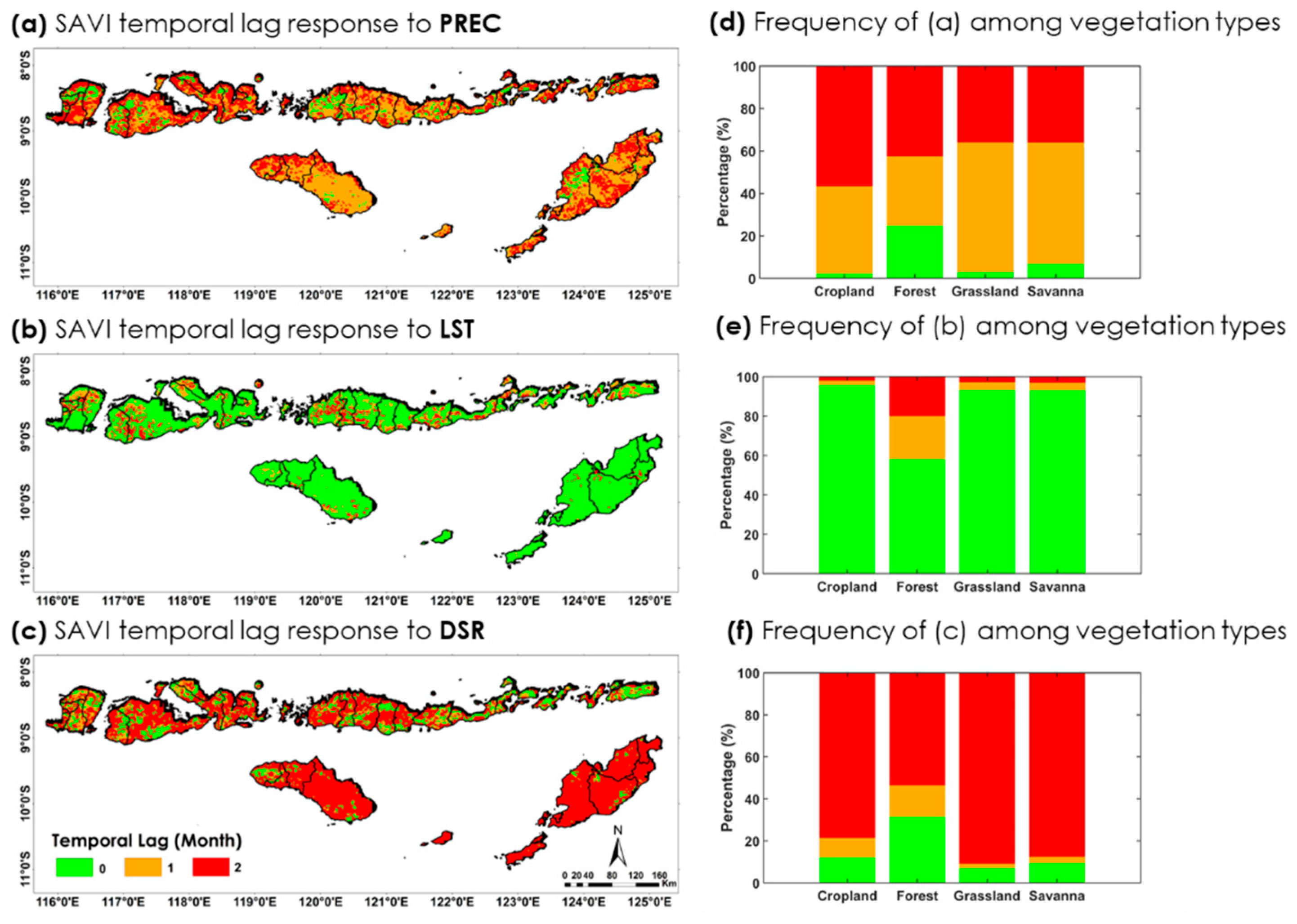
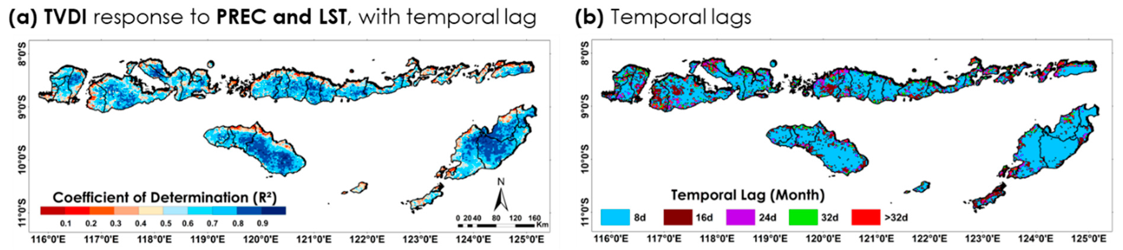
- Partial correlation and time-lag analyses show that LST is the dominant factor affecting the SAVI, with cropland, savanna, and grassland showing the highest sensitivity. In forested areas, however, the influence of meteorological factors was less pronounced, suggesting that other factors may play a greater role in these areas. The factors explained 36−66% of the vegetation variation. Additionally, vegetation shows a rapid response to LST and a 1–2-month time lag in terms of precipitation and DSR. Thus, incorporating the time-lag effect significantly improves the predictive relationship between meteorological factors and changes in vegetation.
- (4)
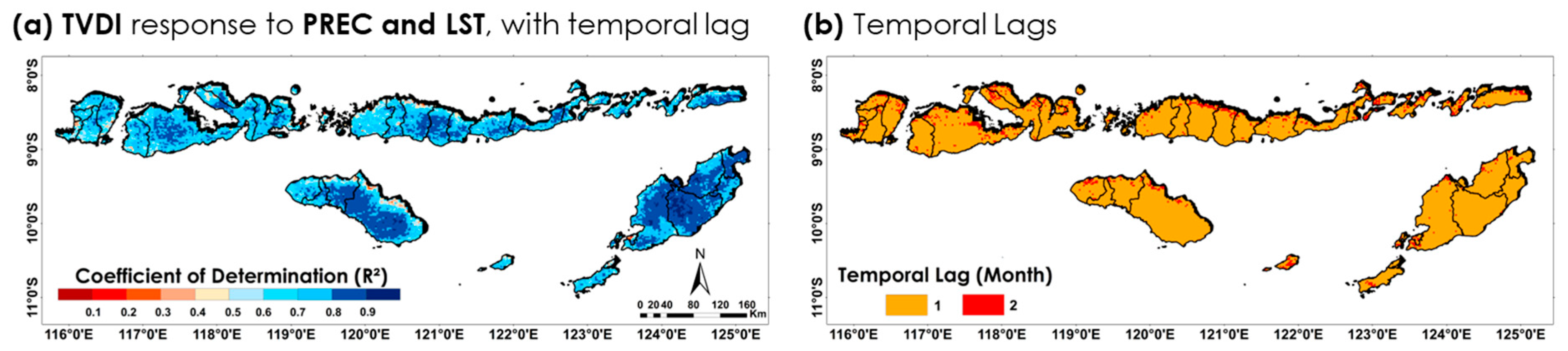
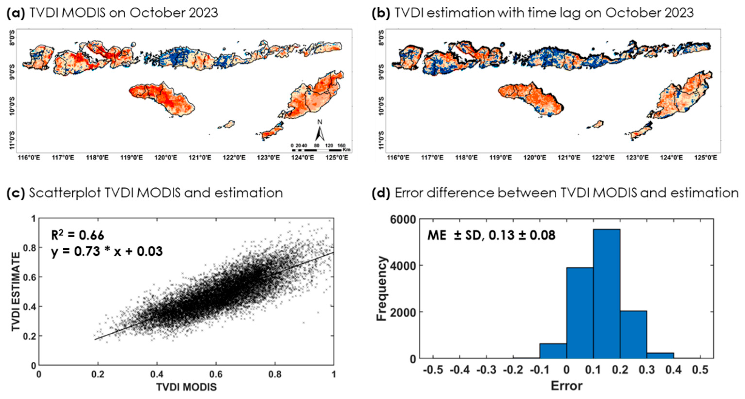
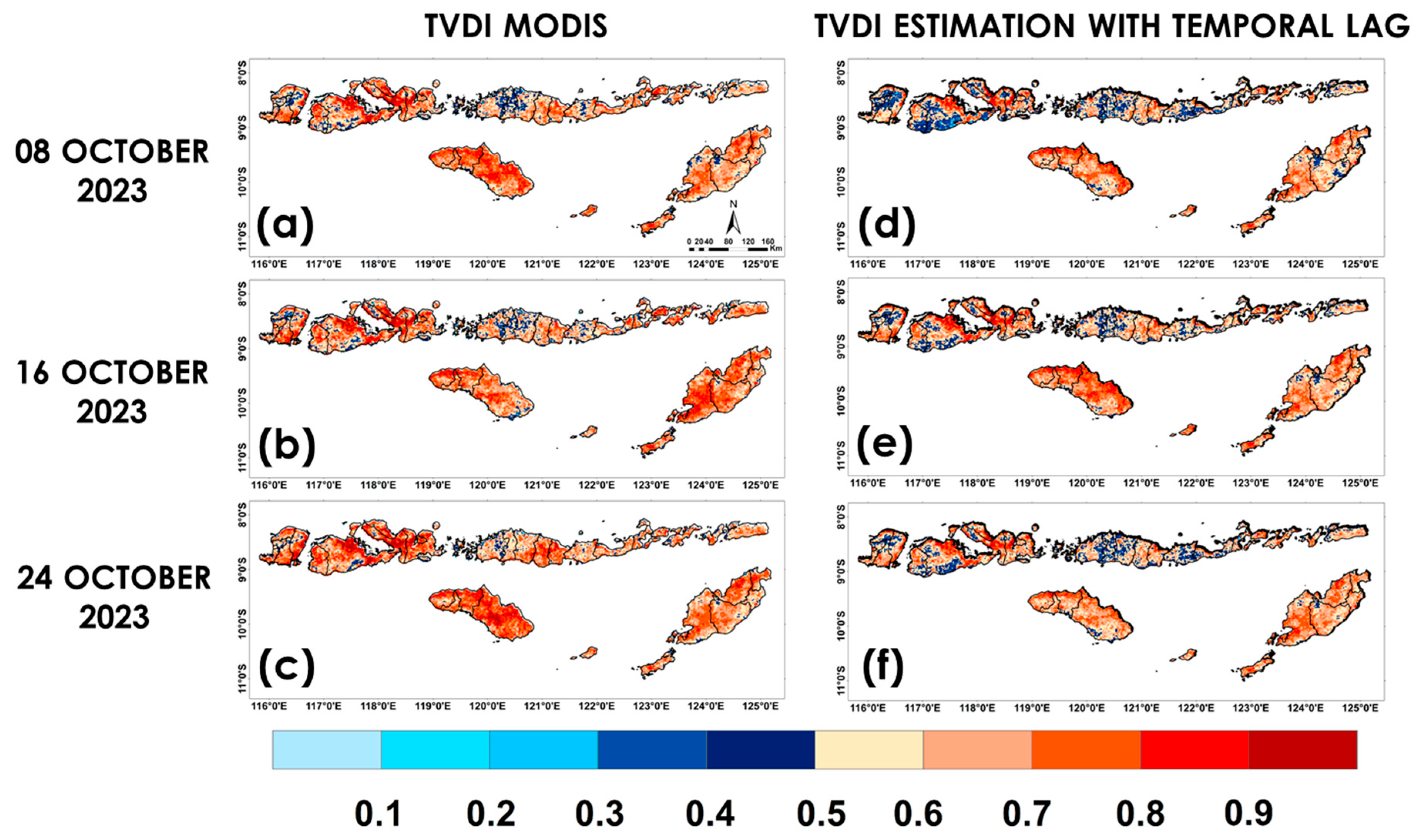
- Regarding agricultural drought estimation, applying MLR models incorporating lagged meteorological inputs proved effective in estimating the TVDI across the NTIs. By selecting PREC and LST as predictors, the monthly and 8-day estimation models could capture spatial drought patterns consistent with MODIS data, with R2 values above 0.64. The low error rates and strong spatial consistency highlight the potential of these models to be accessible tools for predicting agricultural drought.
Author Contributions
Funding
Data Availability Statement
Acknowledgments
Conflicts of Interest
Abbreviations
| NTIs | Nusa Tenggara Islands |
| PREC | Precipitation |
| LST | Land Surface Temperature |
| DSR | Downward Shortwave Radiation |
| NDVI | Normalized-Difference Vegetation Index |
| SAVI | Soil-Adjusted Vegetation Index |
| TVDI | Temperature Vegetation Dryness Index |
| HRE | Himawari-8 rainfall estimation |
| IR | Infrared |
| MVC | Maximum value composite |
| IMSRA | Indian Satellite Multi-Spectral Rainfall Algorithm |
| MLR | Multiple linear regression |
References
- Naveendrakumar, G.; Vithanage, M.; Kwon, H.H.; Chandrasekara, S.S.K.; Iqbal, M.C.M.; Pathmarajah, S.; Fernando, W.C.D.K.; Obeysekera, J. South Asian Perspective on Temperature and Rainfall Extremes: A Review. Atmos. Res. 2019, 225, 110–120. [Google Scholar] [CrossRef]
- Rafiq, M.; Li, Y.C.; Cheng, Y.; Rahman, G.; Ullah, I.; Ali, A. Spatial and Temporal Fluctuation of Rainfall and Drought in Balochistan Province, Pakistan. Arab. J. Geosci. 2022, 15, 214. [Google Scholar] [CrossRef]
- Rahman, G.; Jung, M.K.; Kim, T.W.; Kwon, H.H. Drought Impact, Vulnerability, Risk Assessment, Management and Mitigation under Climate Change: A Comprehensive Review. KSCE J. Civ. Eng. 2025, 29, 100120. [Google Scholar] [CrossRef]
- Xu, C.; McDowell, N.G.; Fisher, R.A.; Wei, L.; Sevanto, S.; Christoffersen, B.O.; Weng, E.; Middleton, R.S. Increasing Impacts of Extreme Droughts on Vegetation Productivity under Climate Change. Nat. Clim. Change 2019, 9, 948–953. [Google Scholar] [CrossRef]
- Orimoloye, I.R. Agricultural Drought and Its Potential Impacts: Enabling Decision-Support for Food Security in Vulnerable Regions. Front. Sustain. Food Syst. 2022, 6, 838824. [Google Scholar] [CrossRef]
- Fang, Y.; Xiong, L. General Mechanisms of Drought Response and Their Application in Drought Resistance Improvement in Plants. Cell. Mol. Life Sci. 2015, 72, 673–689. [Google Scholar] [CrossRef] [PubMed]
- BPS. Statistik Pertanian Provinsi Nusa Tenggara Timur 2023 (Agricultural Statistics of East Nusa Tenggara Province 2023). Available online: https://ntt.bps.go.id/id/publication/2024/09/20/e571dcc6145f7795887626fd/statistik-pertanian-provinsi-nusa-tenggara-timur-2023.html (accessed on 5 April 2025).
- Saidah, H.; Sulistiyono, H.; Negara, I.D.G.J. Comparison of Suitable Drought Indices for Over West Nusa Tenggara. In International Conference on Rehabilitation and Maintenance in Civil Engineering; Lecture Notes in Civil Engineering; Springer: Singapore, 2023; Volume 225, pp. 587–600. [Google Scholar] [CrossRef]
- Adhyani, N.L.; June, T.; Sopaheluwakan, A. Exposure to Drought: Duration, Severity and Intensity (Java, Bali and Nusa Tenggara). IOP Conf. Ser. Earth Environ. Sci. 2017, 58, 012040. [Google Scholar] [CrossRef]
- Kuswanto, H.; Hibatullah, F.; Soedjono, E.S. Perception of Weather and Seasonal Drought Forecasts and Its Impact on Livelihood in East Nusa Tenggara, Indonesia. Heliyon 2019, 5, e02360. [Google Scholar] [CrossRef] [PubMed]
- Tjasyono, B.H.; Gernowo, R.; Sri Woro, B.H. The Character of Rainfall in the Indonesian Monsoon. In Proceedings of the International Symposium on Equatorial Monsoon System, Yogyakarta, Indonesia, 16–18 September 2008. [Google Scholar]
- Ardi, R.D.W.; Aswan; Maryunani, K.A.; Yulianto, E.; Putra, P.S.; Nugroho, S.H.; Istiana. Last Deglaciation—Holocene Australian-Indonesian Monsoon Rainfall Changes Off Southwest Sumba, Indonesia. Atmosphere 2020, 11, 932. [Google Scholar] [CrossRef]
- Wheeler, M.C.; McBride, J.L. Australian-Indonesian Monsoon. In Intraseasonal Variability in the Atmosphere-Ocean Climate System; Springer: Berlin/Heidelberg, Germany, 2005; pp. 125–173. [Google Scholar] [CrossRef]
- Giarno; Hadi, M.P.; Suprayogi, S.; Herumurti, S. Impact of Rainfall Intensity, Monsoon and MJO to Rainfall Merging in the Indonesian Maritime Continent. J. Earth Syst. Sci. 2020, 129, 164. [Google Scholar] [CrossRef]
- Matsumoto, J.; Wang, B.; Wu, G.; Li, J.; Wu, P.; Hattori, M.; Mori, S.; Yamanaka, M.D.; Ogino, S.Y.; Jun-Ichi, H.; et al. An Overview of the Asian Monsoon Years 2007–2012 (AMY) and Multi-Scale Interactions in the Extreme Rainfall Events over the Indonesian Maritime Continent. World Sci. Ser. Asia-Pac. Weather Clim. 2017, 9, 365–385. [Google Scholar] [CrossRef]
- Kirono, D.G.C. Principal Component Analysis for Identifying Period of Seasons in Indonesia. Indones. J. Geogr. 2004, 36, 109–121. [Google Scholar] [CrossRef]
- Kirono, D.G.C.; Butler, J.R.A.; McGregor, J.L.; Ripaldi, A.; Katzfey, J.; Nguyen, K. Historical and Future Seasonal Rainfall Variability in Nusa Tenggara Barat Province, Indonesia: Implications for the Agriculture and Water Sectors. Clim. Risk Manag. 2016, 12, 45–58. [Google Scholar] [CrossRef]
- Sanit, M.S.; Rachmawati, T.A.; Firdausiyah, N. Impact of Climate Change on Meteorological Drought in Insana Barat District, Timor Tengah Utara, East Nusa Tenggara. J. Syntax. Lit. 2023, 8, 417–425. [Google Scholar] [CrossRef]
- Kusmiyarti, T.B.; Adnyana, W.S.; Nuarsa, W.; Sudarma, M.; Antara, M.O.G. Drought Monitoring Using Remote Sensing Data in Nusa Tenggara Timur Province, Indonesia in Between 2018 and 2023. Ecol. Eng. Environ. Technol. 2024, 25, 134–145. [Google Scholar] [CrossRef]
- Setiawan, A.M.; Lee, W.S.; Rhee, J. Spatio-Temporal Characteristics of Indonesian Drought Related to El Niño Events and Its Predictability Using the Multi-Model Ensemble. Int. J. Climatol. 2017, 37, 4700–4719. [Google Scholar] [CrossRef]
- Rahman As-syakur, A.; Wayan Sandi Adnyana, I.; Sudiana Mahendra, M.; Wayan Arthana, I.; Nyoman Merit, I.; Wayan Kasa, I.; Wayan Ekayanti, N.; Wayan Nuarsa, I.; Nyoman Sunarta, I. Observation of Spatial Patterns on the Rainfall Response to ENSO and IOD over Indonesia Using TRMM Multisatellite Precipitation Analysis (TMPA). Int. J. Climatol. 2014, 34, 3825–3839. [Google Scholar] [CrossRef]
- Karuniasa, M.; Pambudi, P.A. The Analysis of the El Niño Phenomenon in the East Nusa Tenggara Province, Indonesia. J. Water Land. Dev. 2022, 52, 180–185. [Google Scholar] [CrossRef]
- Nemani, R.R.; Keeling, C.D.; Hashimoto, H.; Jolly, W.M.; Piper, S.C.; Tucker, C.J.; Myneni, R.B.; Running, S.W. Climate-Driven Increases in Global Terrestrial Net Primary Production from 1982 to 1999. Science 2003, 300, 1500–1563. [Google Scholar] [CrossRef] [PubMed]
- Matuszko, D.; Library, W.O. Influence of the Extent and Genera of Cloud Cover on Solar Radiation Intensity. Int. J. Climatol. 2012, 32, 2403–2414. [Google Scholar] [CrossRef]
- Zhao, M.; A, G.; Liu, Y.; Konings, A.G. Evapotranspiration Frequently Increases during Droughts. Nat. Clim. Change 2022, 12, 1024–1030. [Google Scholar] [CrossRef]
- Chen, Z.; Wang, W.; Fu, J. Vegetation Response to Precipitation Anomalies under Different Climatic and Biogeographical Conditions in China. Sci. Rep. 2020, 10, 830. [Google Scholar] [CrossRef] [PubMed]
- Wu, D.; Zhao, X.; Zhao, W.; Tang, B.; Xu, W. Response of Vegetation to Temperature, Precipitation and Solar Radiation Time-Scales: A Case Study over Mainland Australia. In Proceedings of the International Geoscience and Remote Sensing Symposium (IGARSS), Quebec City, QC, Canada, 13–18 July 2014; pp. 855–858. [Google Scholar] [CrossRef]
- Ren, H.; Wen, Z.; Liu, Y.; Lin, Z.; Han, P.; Shi, H.; Wang, Z.; Su, T. Vegetation Response to Changes in Climate across Different Climate Zones in China. Ecol. Indic. 2023, 155, 110932. [Google Scholar] [CrossRef]
- Li, X.; Qu, Y. Evaluation of Vegetation Responses to Climatic Factors and Global Vegetation Trends Using GLASS LAI from 1982 to 2010. Can. J. Remote Sens. 2018, 44, 357–372. [Google Scholar] [CrossRef]
- Ma’Rufah, U.; Hidayat, R.; Prasasti, I. Analysis of Relationship between Meteorological and Agricultural Drought Using Standardized Precipitation Index and Vegetation Health Index. IOP Conf. Ser. Earth Environ. Sci. 2017, 54, 012008. [Google Scholar] [CrossRef]
- Piao, S.; Cui, M.; Chen, A.; Wang, X.; Ciais, P.; Liu, J.; Tang, Y. Altitude and Temperature Dependence of Change in the Spring Vegetation Green-up Date from 1982 to 2006 in the Qinghai-Xizang Plateau. Agric. For. Meteorol. 2011, 151, 1599–1608. [Google Scholar] [CrossRef]
- Tao, Z.; Wang, H.; Liu, Y.; Xu, Y.; Dai, J. Phenological Response of Different Vegetation Types to Temperature and Precipitation Variations in Northern China during 1982–2012. Int. J. Remote Sens. 2017, 38, 3236–3252. [Google Scholar] [CrossRef]
- Varma, A.K. Measurement of Precipitation from Satellite Radiometers (Visible, Infrared, and Microwave): Physical Basis, Methods, and Limitations. In Remote Sensing of Aerosols, Clouds, and Precipitation; Elsevier: Amsterdam, The Netherlands, 2018; pp. 223–248. [Google Scholar] [CrossRef]
- Wan, Z.; Li, Z.L. Radiance-based Validation of the V5 MODIS Land-surface Temperature Product. Int. J. Remote Sens. 2008, 29, 5373–5395. [Google Scholar] [CrossRef]
- Wan, Z.; Zhang, Y.; Zhang, Q.; Li, Z. liang Validation of the Land-Surface Temperature Products Retrieved from Terra Moderate Resolution Imaging Spectroradiometer Data. Remote Sens. Environ. 2002, 83, 163–180. [Google Scholar] [CrossRef]
- Wang, D.; Liang, S.; Zhang, Y.; Gao, X.; Brown, M.G.L.; Jia, A. A New Set of Modis Land Products (Mcd18): Downward Shortwave Radiation and Photosynthetically Active Radiation. Remote Sens. 2020, 12, 168. [Google Scholar] [CrossRef]
- Wan, Z. New Refinements and Validation of the MODIS Land-Surface Temperature/Emissivity Products. Remote Sens. Environ. 2008, 112, 59–74. [Google Scholar] [CrossRef]
- Sharma, R.C.; Hara, K.; Hirayama, H. Improvement of Countrywide Vegetation Mapping over Japan and Comparison to Existing Maps. Adv. Remote Sens. 2018, 7, 163–170. [Google Scholar] [CrossRef]
- Liang, D.; Zuo, Y.; Huang, L.; Zhao, J.; Teng, L.; Yang, F. Evaluation of the Consistency of MODIS Land Cover Product (MCD12Q1) Based on Chinese 30 m GlobeLand30 Datasets: A Case Study in Anhui Province, China. ISPRS Int. J. Geo-Inf. 2015, 4, 2519–2541. [Google Scholar] [CrossRef]
- Kumparan Kondisi Geografis Pulau Bali dan Nusa Tenggara Berdasarkan Peta|kumparan.com. Available online: https://kumparan.com/kabar-harian/kondisi-geografis-pulau-bali-dan-nusa-tenggara-berdasarkan-peta-22d0HEcXhkq (accessed on 7 April 2025).
- Silaen, M.; Yuwono, Y.; Ismail, C.; Ramadhani, A.; Takama, T. Vulnerability Assessment on Agriculture in East Nusa Tenggara. In Climate Change Management; Springer: Cham, Switzerland, 2023; Part F5; pp. 109–134. [Google Scholar] [CrossRef]
- Kuswanto, H.; Puspa, A.W.; Ahmad, I.S.; Hibatullah, F. Drought Analysis in East Nusa Tenggara (Indonesia) Using Regional Frequency Analysis. Sci. World J. 2021, 2021, 6626102. [Google Scholar] [CrossRef] [PubMed]
- Schneider, U.; Becker, A.; Finger, P.; Meyer-Christoffer, A.; Rudolf, B.; Ziese, M. GPCC’s new land surface precipitation climatology based on quality-controlled in situ data and its role in quantifying the global water cycle. Theor. Appl. Climatol. 2014, 115, 15–40. [Google Scholar] [CrossRef]
- Bessho, K.; Date, K.; Hayashi, M.; Ikeda, A.; Imai, T.; Inoue, H.; Kumagai, Y.; Miyakawa, T.; Murata, H.; Ohno, T.; et al. An Introduction to Himawari-8/9—Japan’s New-Generation Geostationary Meteorological Satellites. J. Meteorol. Soc. Jpn. 2016, 94, 151–183. [Google Scholar] [CrossRef]
- Wan, Z. Collection-6 MODIS Land Surface Temperature Products Users’ Guide. 2013. Available online: https://lpdaac.usgs.gov/documents/118/MOD11_User_Guide_V6.pdf (accessed on 10 April 2025).
- Roger, J.C.; Ray, J.P.; Vermote, E.F. MODIS Surface Reflectance User’s Guide. 2023. Available online: https://ladsweb.modaps.eosdis.nasa.gov/archive/Document%20Archive/Science%20Data%20Product%20Documentation/MOD09_C61_UserGuide_v1.7.pdf (accessed on 10 April 2025).
- Sulla-Menashe, D.; Friedl, M.A. User Guide to Collection 6 MODIS Land Cover (MCD12Q1 and MCD12C1) Product. 2018. Available online: https://modis-land.gsfc.nasa.gov/pdf/MCD12Q1_C6_Userguide04042018.pdf (accessed on 10 April 2025).
- Holben, B.N. Characteristics of Maximum-Value Composite Images from Temporal AVHRR Data. Int. J. Remote Sens. 1986, 7, 1417–1434. [Google Scholar] [CrossRef]
- Prakash, S.; Mishra, A.; Gairola, R.; Varma, A.; Pal, P. Combined Use of Microwave and IR Data for The Study of Indian Monsoon Rainfall-2009. In Proceedings of the ISPRS Archives XXXVIII-8/W3 Workshop Proceedings: Impact of Climate Change on Agriculture, Ahmedabad, India, 17–18 December 2009. [Google Scholar]
- Sobajima, A. Rapidly Developing Cumulus Areas Derivation Algorithm Theoretical Basis Document. 2012. Available online: https://cwg.eumetsat.int/2013/01/jmas-rapidly-developing-cumulus-areas-algorithm/ (accessed on 5 March 2025).
- Huete, A.R. A Soil-Adjusted Vegetation Index (SAVI). Remote Sens. Environ. 1988, 25, 295–309. [Google Scholar] [CrossRef]
- Sandholt, I.; Rasmussen, K.; Andersen, J. A Simple Interpretation of the Surface Temperature/Vegetation Index Space for Assessment of Surface Moisture Status. Remote Sens. Environ. 2002, 79, 213–224. [Google Scholar] [CrossRef]
- He, Y.; Chen, F.; Jia, H.; Wang, L.; Bondur, V.G. Different Drought Legacies of Rain-Fed and Irrigated Croplands in a Typical Russian Agricultural Region. Remote Sens. 2020, 12, 1700. [Google Scholar] [CrossRef]
- Li, W. Classification of Drought Grades Based on Temperature Vegetation Drought Index Using the MODIS Data. Res. Soil Water Conserv. 2017, 24, 130–135. [Google Scholar]
- McKee, T.B.; Doesken, N.J.; Kleist, J. The relationship of drought frequency and duration to time scales. In Proceedings of the Eighth Conference on Applied Climatology, Anaheim, CA, USA, 17–22 January 1993; pp. 17–22. [Google Scholar]
- Liu, C.; Yang, C.; Yang, Q.; Wang, J. Spatiotemporal Drought Analysis by the Standardized Precipitation Index (SPI) and Standardized Precipitation Evapotranspiration Index (SPEI) in Sichuan Province, China. Sci. Rep. 2021, 11, 1280. [Google Scholar] [CrossRef] [PubMed]
- Kendall, M.G. Partial Rank Correlation. Biometrika 1942, 32, 277–283. [Google Scholar] [CrossRef]
- Niu, Y.S.; Hao, N.; Zhang, H.H. Interaction Screening by Partial Correlation. Stat. Interface 2018, 11, 317–325. [Google Scholar] [CrossRef]
- Wu, D.; Zhao, X.; Liang, S.; Zhou, T.; Huang, K.; Tang, B.; Zhao, W. Time-Lag Effects of Global Vegetation Responses to Climate Change. Glob. Change Biol. 2015, 21, 3520–3531. [Google Scholar] [CrossRef] [PubMed]
- Apriyana, Y.; Surmaini, E.; Estiningtyas, W.; Pramudia, A.; Ramadhani, F.; Suciantini, S.; Susanti, E.; Purnamayani, R.; Syahbuddin, H. The Integrated Cropping Calendar Information System: A Coping Mechanism to Climate Variability for Sustainable Agriculture in Indonesia. Sustainability 2021, 13, 6495. [Google Scholar] [CrossRef]
- Hayashi, K.; Bugayong, I.; Siregar, I.H.; Jonharnas; Wirajaswadi, L.; Hadiawati, L.; Agustiani, N.; Orden, M.E. Appraisal of Rainfed Rice Production and Management Practices through Case Studies in North Sumatera and West Nusa Tenggara, Indonesia. Trop. Agric. Dev. 2018, 62, 43–54. [Google Scholar] [CrossRef]
- Meliani, F.; Sulistyowati, R.; Permata, Z.D.O.; Sumargana, L.; Amaliyah, R.; Purwandani, A.; Putrantijo, N.; Ramadhan, A.R. Preliminary Study on Validation of HIMAWARI-8 Data with Ground Based Rainfall Data at South Sumatera, Indonesia. IOP Conf. Ser. Earth Environ. Sci. 2020, 500, 012031. [Google Scholar] [CrossRef]
- Ismanto, R.D.; Prasasti, I.; Fitriana, H.L. Comparison Analysis of Himawari 8, CHIRPS and GSMaP Data to Detect Rain in Indonesia. J. Meteorol. Dan. Geofis. 2023, 24, 9–17. [Google Scholar] [CrossRef]
- Mishra, A.; Gairola, R.; Varma, A.; Agarwal, V.K. Study of Intense Rainfall Events over India Using Kalpana-IR and TRMM-Precipitation Radar Observations. Curr. Sci. 2009, 97, 689–695. Available online: https://www.jstor.org/stable/24112165 (accessed on 5 March 2025).
- Lei, H.; Li, H.; Zhao, H.; Ao, T.; Li, X. Comprehensive Evaluation of Satellite and Reanalysis Precipitation Products over the Eastern Tibetan Plateau Characterized by a High Diversity of Topographies. Atmos. Res. 2021, 259, 105661. [Google Scholar] [CrossRef]
- Bhattarai, S.; Talchabhadel, R. Comparative Analysis of Satellite-Based Precipitation Data across the CONUS and Hawaii: Identifying Optimal Satellite Performance. Remote Sens. 2024, 16, 3058. [Google Scholar] [CrossRef]
- Nasrollahi, N. Reducing False Rain in Satellite Precipitation Products Using Cloudsat Cloud Classification Maps and Modis Multi-Spectral Images. In Improving Infrared-Based Precipitation Retrieval Algorithms Using Multi-Spectral Satellite Imagery; Springer Theses; Springer: Cham, Switzerland, 2015; pp. 21–32. [Google Scholar] [CrossRef]
- Vicente-Serrano, S.M.; Gouveia, C.; Camarero, J.J.; Beguería, S.; Trigo, R.; López-Moreno, J.I.; Azorín-Molina, C.; Pasho, E.; Lorenzo-Lacruz, J.; Revuelto, J.; et al. Response of Vegetation to Drought Time-Scales across Global Land Biomes. Proc. Natl. Acad. Sci. USA 2013, 110, 52–57. [Google Scholar] [CrossRef] [PubMed]
- Wang, C.; Chen, J.; Lee, S.C.; Xiong, L.; Su, T.; Lin, Q.; Xu, C.Y. Response and Recovery Times of Vegetation Productivity under Drought Stress: Dominant Factors and Relationships. J. Hydrol. 2025, 655, 132945. [Google Scholar] [CrossRef]
- Huffman, G.J.; Bolvin, D.T.; Braithwaite, D.; Hsu, K.L.; Joyce, R.J.; Kidd, C.; Nelkin, E.J.; Sorooshian, S.; Stocker, E.F.; Tan, J.; et al. Integrated Multi-Satellite Retrievals for the Global Precipitation Measurement (GPM) Mission (IMERG). In Satellite Precipitation Measurement; Advances in Global Change Research; Springer: Cham, Switzerland, 2020; Volume 67, pp. 343–353. [Google Scholar] [CrossRef]
- Funk, C.; Peterson, P.; Landsfeld, M.; Pedreros, D.; Verdin, J.; Shukla, S.; Husak, G.; Rowland, J.; Harrison, L.; Hoell, A.; et al. The Climate Hazards Infrared Precipitation with Stations—A New Environmental Record for Monitoring Extremes. Sci. Data 2015, 2, 150066. [Google Scholar] [CrossRef] [PubMed]
- Ashouri, H.; Hsu, K.L.; Sorooshian, S.; Braithwaite, D.K.; Knapp, K.R.; Cecil, L.D.; Nelson, B.R.; Prat, O.P. PERSIANN-CDR: Daily Precipitation Climate Data Record from Multisatellite Observations for Hydrological and Climate Studies. Bull. Am. Meteorol. Soc. 2015, 96, 69–83. [Google Scholar] [CrossRef]
- Suriadi, A.; Mulyani, A.; Hadiawati, L.; Suratman. Biophysical Characteristics of Dry-Climate Upland and Agriculture Development Challenges in West Nusa Tenggara and East Nusa Tenggara Provinces. IOP Conf. Ser. Earth Environ. Sci. 2021, 648, 012014. [Google Scholar] [CrossRef]
- Selvaraj, J.; Marimuthu, P.D. Modeling Vegetation Dynamics: Insights from Distributed Lag Model and Spatial Interpolation of Satellite Derived Environmental Data. In International Conference on Mathematics and Computing; Lecture Notes in Networks and Systems; Springer: Singapore, 2024; Volume 963, pp. 41–51. [Google Scholar] [CrossRef]

| Dataset | Temporal Resolution | Spatial Resolution | Input Parameter | Data Source |
|---|---|---|---|---|
| Himawari-8 (AHI 1) | 10 min | 2 km | Thermal infrared: B13 (10.4 µm), B15 (12.4 µm) | JAXA 3 (https://www.eorc.jaxa.jp/ptree/index.html, accessed on 15 September 2024) |
| Rain Gauge | 1 day | - | Surface precipitation observation | Indonesia Meteorological Agency (https://dataonline.bmkg.go.id/, accessed on 15 September 2024) |
| MODIS 2: MOD11A2.061 | 8 days | 1 km | Land surface temperature | NASA 4 (https://lpdaac.usgs.gov/, accessed on 15 September 2024) |
| MODIS: MOD09A1.061 | 8 days | 0.5 km | Surface reflectance bands 1 and 2 | |
| MODIS: MCD18A1.061 | 1 day | 1 km | Downward Surface Radiation | |
| MODIS: MCD12Q1.061 | Yearly | 0.5 km | Land-cover classification |
| TVDI | Drought Class | Soil Moisture Status |
|---|---|---|
| 0 < TVDI < 0.46 | No drought | Surface water is sufficient or normal |
| 0.46 < TVDI < 0.57 | Mild drought | Small amount of surface evaporation and dry air near the surface |
| 0.57 < TVDI < 0.76 | Moderate drought | The soil surface is dry, and vegetation leaves are wilting |
| 0.76 < TVDI < 0.86 | Severe drought | Thicker dry soil layers appear, and vegetation is withered |
| 0.86 < TVDI < 1 | Extreme drought | Surface vegetation is dry or dead |
| Metrics | Formula | Range | Optimum |
|---|---|---|---|
| Critical success index (CSI) | [0, 1] | 1 | |
| Probability of detection (POD) | [0, 1] | 1 | |
| False-alarm ratio (FAR) | [0, 1] | 0 | |
| Coefficient of determination (R2) | [0, 1] | 1 | |
| Normalized root mean square error (NRMSE) | [0, 1] | 0 | |
| Normalized mean bias error (NMBE) | [−1, 1] | 0 |
| Partial Corr. (Mean ± 95% CI) | Vegetation Types | |||
|---|---|---|---|---|
| Cropland | Forest | Grassland | Savanna | |
| SAVI-PREC | 0.14 ± 0.0136 | 0.04 ± 0.0099 | 0.30 ± 0.0155 | 0.23 ± 0.0080 |
| SAVI-LST | (−0.71) ± 0.0108 | (−0.23) ± 0.0113 | (−0.67) ± 0.0114 | (−0.65) ± 0.0060 |
| SAVI-DSR | 0.38 ± 0.0100 | 0.13 ± 0.0063 | 0.33 ± 0.0130 | 0.34 ± 0.0055 |
| Corr. (Mean ± 95% CI) | Vegetation Types | |||
|---|---|---|---|---|
| Cropland | Forest | Grassland | Savanna | |
| SAVI-SPI-1 | 0.45 ± 0.0105 | 0.17 ± 0.0115 | 0.53 ± 0.0109 | 0.51 ± 0.0069 |
| SAVI-SPI-3 | 0.64 ± 0.0111 | 0.31 ± 0.0117 | 0.71 ± 0.0100 | 0.68 ± 0.0067 |
| Partial Corr. (Mean ± 95% CI) | Vegetation Types | |||
|---|---|---|---|---|
| Cropland | Forest | Grassland | Savanna | |
| TVDI-PREC | (−0.20) ± 0.0112 | (−0.29) ± 0.0065 | (−0.10) ± 0.0137 | (−0.23) ± 0.0062 |
| TVDI-LST | 0.75 ± 0.0052 | 0.74 ± 0.0029 | 0.71 ± 0.0076 | 0.78 ± 0.0026 |
| TVDI-DSR | (−0.21) ± 0.0145 | 0.07 ± 0.0073 | (−0.11) ± 0.0154 | 0.02 ± 0.0084 |
| Partial Corr. (Mean ± 95% CI) | Vegetation Types | |||
|---|---|---|---|---|
| Cropland | Forest | Grassland | Savanna | |
| TVDI-SPI-1 | (−0.39) ± 0.0113 | (−0.29) ± 0.0076 | (−0.33) ± 0.0140 | (−0.39) ± 0.0070 |
| TVDI-SPI-3 | (−0.53) ± 0.0110 | (−0.37) ± 0.0071 | (−0.44) ± 0.0132 | (−0.54) ± 0.0060 |
| LST-SPI-1 | (−0.33) ± 0.0088 | (−0.20) ± 0.0068 | (−0.33) ± 0.0090 | (−0.34) ± 0.0055 |
| LST-SPI-3 | (−0.57) ± 0.0081 | (−0.39) ± 0.0067 | (−0.55) ± 0.0074 | (−0.57) ± 0.0044 |
| Date | Metrics Evaluation | |||
|---|---|---|---|---|
| Regression | R2 | NRMSE | NMBE | |
| 8 October 2023 | y = 0.85 * x + 0.04 | 0.69 | 0.09 | 0.05 |
| 16 October 2023 | y = 0.78 * x + 0.11 | 0.67 | 0.07 | 0.03 |
| 24 October 2023 | y = 0.77 * x + 0.09 | 0.64 | 0.09 | 0.07 |
Disclaimer/Publisher’s Note: The statements, opinions and data contained in all publications are solely those of the individual author(s) and contributor(s) and not of MDPI and/or the editor(s). MDPI and/or the editor(s) disclaim responsibility for any injury to people or property resulting from any ideas, methods, instructions or products referred to in the content. |
© 2025 by the authors. Licensee MDPI, Basel, Switzerland. This article is an open access article distributed under the terms and conditions of the Creative Commons Attribution (CC BY) license (https://creativecommons.org/licenses/by/4.0/).
Share and Cite
Krisnawan, G.D.; Chang, Y.-L.; Tsai, F.; Tseng, K.-H.; Lin, T.-H. Meteorological Drivers and Agricultural Drought Diagnosis Based on Surface Information and Precipitation from Satellite Observations in Nusa Tenggara Islands, Indonesia. Remote Sens. 2025, 17, 2460. https://doi.org/10.3390/rs17142460
Krisnawan GD, Chang Y-L, Tsai F, Tseng K-H, Lin T-H. Meteorological Drivers and Agricultural Drought Diagnosis Based on Surface Information and Precipitation from Satellite Observations in Nusa Tenggara Islands, Indonesia. Remote Sensing. 2025; 17(14):2460. https://doi.org/10.3390/rs17142460
Chicago/Turabian StyleKrisnawan, Gede Dedy, Yi-Ling Chang, Fuan Tsai, Kuo-Hsin Tseng, and Tang-Huang Lin. 2025. "Meteorological Drivers and Agricultural Drought Diagnosis Based on Surface Information and Precipitation from Satellite Observations in Nusa Tenggara Islands, Indonesia" Remote Sensing 17, no. 14: 2460. https://doi.org/10.3390/rs17142460
APA StyleKrisnawan, G. D., Chang, Y.-L., Tsai, F., Tseng, K.-H., & Lin, T.-H. (2025). Meteorological Drivers and Agricultural Drought Diagnosis Based on Surface Information and Precipitation from Satellite Observations in Nusa Tenggara Islands, Indonesia. Remote Sensing, 17(14), 2460. https://doi.org/10.3390/rs17142460