Laser-Induced Breakdown Spectroscopy Quantitative Analysis Using a Bayesian Optimization-Based Tunable Softplus Backpropagation Neural Network

Abstract

Laser-induced breakdown spectroscopy (LIBS) has played a critical role in Mars exploration missions, substantially contributing to the geochemical analysis of Martian surface substances. However, the complex nonlinearity of LIBS processes can considerably limit the quantification accuracy of conventional LIBS chemometric methods. Hence chemometrics based on artificial neural network (ANN) algorithms have become increasingly popular in LIBS analysis due to their extraordinary ability in nonlinear feature modeling. The hidden layer activation functions are key to ANN model performance, yet common activation functions usually suffer from problems such as gradient vanishing (e.g., Sigmoid and Tanh) and dying neurons (e.g., ReLU). In this study, we propose a novel LIBS quantification method, named the Bayesian optimization-based tunable Softplus backpropagation neural network (BOTS-BPNN). Based on a dataset comprising 1800 LIBS spectra collected by a laboratory duplicate of the MarSCoDe instrument onboard the Zhurong Mars rover, we have revealed that a BPNN model adopting a tunable Softplus activation function can achieve higher prediction accuracy than BPNN models adopting other common activation functions if the tunable Softplus parameter β is properly selected. Moreover, the way to find the proper β value has also been investigated. We demonstrate that the Bayesian optimization method surpasses the traditional grid search method regarding both performance and efficiency. The BOTS-BPNN model also shows superior performance over other common machine learning models like random forest (RF). This work indicates the potential of BOTS-BPNN as an effective chemometric method for analyzing Mars in situ LIBS data and sheds light on the use of chemometrics for data analysis in future planetary explorations.

1. Introduction

During China’s Tianwen-1 Mars mission, the Zhurong rover successfully landed in the Utopia Planitia region on Mars to investigate the planet’s environment, including geomorphological features, the chemical composition of surface materials, etc. On the Zhurong rover, the major scientific payload for material composition detection is MarSCoDe, an instrument that utilizes the laser-induced breakdown spectroscopy (LIBS) technique [1].

As a kind of atomic emission spectroscopic technique, LIBS uses high-energy laser pulses to induce material melting, vaporization, atomic ionization, and plasma generation. The spectral signal originating from plasma radiation, consisting of fingerprint information of the elements, allows researchers to perform both qualitative and quantitative analyses of the material composition. In comparison to conventional elemental analysis methods like atomic absorption spectroscopy (AAS) and X-ray fluorescence spectroscopy (XRF) [2,3], LIBS offers several special merits, including minimal sample preparation requirements, the ability to perform stand-off field detection, and the capability to clear surface dust and realize depth profiling, just to name a few. The synergistic combination of these advantages makes LIBS an outstanding analytical tool for Mars surface composition detection. Following NASA’s ChemCam and SuperCam instruments [4,5,6], MarSCoDe has become the third LIBS-powered payload effectively deployed for Mars exploration. Through the interpretation of the chemical composition of Martian rocks and soils, a series of scientific achievements have been made based on the MarSCoDe LIBS data [7,8].

Despite the strong detection capability of the LIBS technique, it can be a challenging task to realize high accuracy in LIBS data analysis, especially quantitative analysis. In principle, the unsatisfactory accuracy is caused by one or more of three key factors: (i) physical and/or chemical matrix effects [9,10], (ii) saturation effects manifested by self-absorption [11,12], and (iii) the relatively low stability and repeatability of LIBS signals due to their sensitivity to fluctuations in experimental conditions [13,14,15]. These nonlinear interfering effects can largely limit the power of conventional linear chemometrics, such as the calibration curve [16], principal component regression (PCR) [17,18], and partial least squares regression (PLSR) [19,20,21]. Hence, nowadays, many LIBS researchers draw support from nonlinear chemometrics, including support vector machine (SVM) [22,23], random forest (RF) [24,25], artificial neural networks (ANNs) [26,27,28], and so on. Specifically, with the boom of deep learning technology in the past decade, ANNs have become increasingly attractive in a broad range of technical communities, including the LIBS community. Since an ANN is suitable for solving problems that are complex, ill-defined, or highly nonlinear, have many different variables, and/or are stochastic, it is veritably a powerful tool for LIBS data analysis [29].

One of the most important ANN paradigms is the so-called backpropagation neural network (BPNN). The BPNN is so far the most widely used ANN scheme in LIBS studies, although there are also several other types of neural networks appreciated by the LIBS community, e.g., radial basis function neural networks (RBFNNs) [30], convolutional neural networks (CNNs) [31,32], self-organizing maps (SOMs) [33], etc. A typical BPNN has an input layer, a hidden layer, and an output layer. One of the most crucial hyperparameters that can affect BPNN model performance is the activation function of the hidden layer. Common activation functions include Tanh, Sigmoid, ReLU, Softplus, and so forth. The Sigmoid and Tanh functions are prone to suffering from the gradient vanishing problem, the ReLU function and its variants may suffer from the gradient explosion problem, and the ReLU function is particularly notorious for the dying neuron problem. Although the Softplus function has a relatively low risk of encountering the above three problems, its form is also fixed and has poor flexibility and adaptability. These problems may hinder the convergence efficiency and prediction accuracy of the BPNN model when analyzing complicated LIBS data.

In this study, we propose a novel BPNN model for LIBS quantification, named the Bayesian optimization-based tunable Softplus backpropagation neural network (BOTS-BPNN). The activation function of the BPNN model is a tunable Softplus function, which differs from the ordinary Softplus function by incorporating a tunable hyperparameter β. While maintaining the merits of the ordinary Softplus function, this tunable Softplus function enables the BPNN model to have stronger flexibility and adaptability. Moreover, we utilize the Bayesian optimization method, instead of the traditional grid search method, to search for the optimal β value in an efficient way.

In order to demonstrate the effectiveness of the proposed methodology, we employ a dataset comprising 1800 LIBS spectra from 30 geochemical samples collected by a laboratory duplicate of the MarSCoDe instrument and take the quantification of the Mg (in the form of MgO within the geochemical samples) concentration as an example. Mg is a key element in the Martian crust, widely distributed in surface and near-surface geological formations, and MgO commonly occurs in primary igneous minerals like olivine and pyroxene, with an average abundance of approximately 8.93 ± 0.45 wt.% in Martian soils [34,35]. In the warm, humid environments hypothesized for early Mars, Mg may have reacted with water to form secondary minerals such as carbonates and sulfates [36]. As such, the Mg abundance may not only reflect crustal composition but also indicate past hydrological processes and climate evolution. Therefore, selecting Mg (MgO) as the illustrative component for quantification is scientifically valuable in the geological and geochemical research of Mars.

In the following text, the LIBS experiment, dataset, and BOTS-BPNN methodology are described in Section 2. In Section 3, we present and explain the results, followed by a detailed discussion in Section 4. The conclusion can be found in Section 5.

2. Materials and Methods

2.1. Experimental Setup

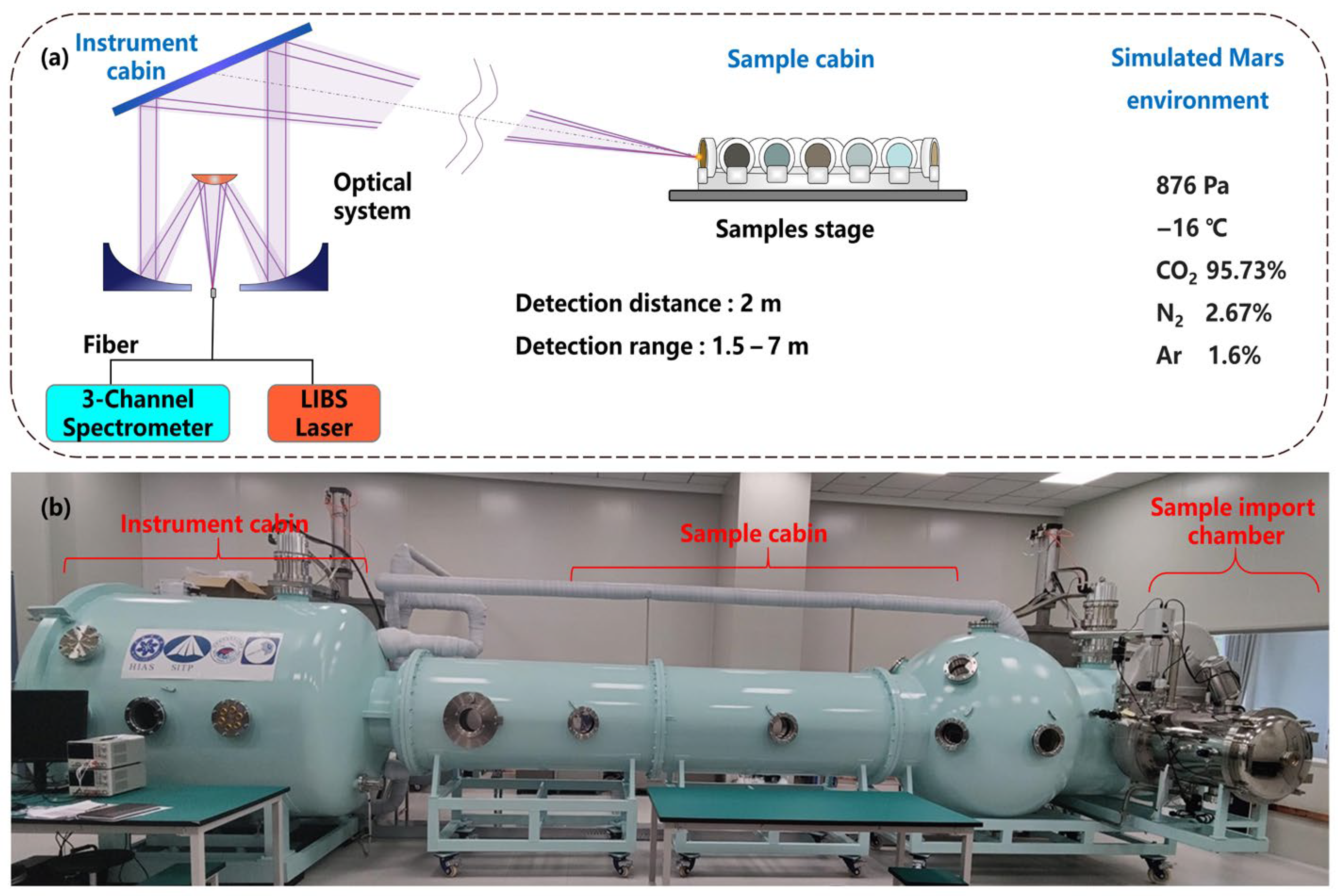
The LIBS instrument used in this study is a laboratory duplicate of the MarSCoDe payload onboard the Zhurong Mars rover. All the LIBS spectra were collected in an environment simulating the Martian atmosphere, based on a specially customized facility called Mars-Simulated Detection Environment Experiment Platform (MarSDEEP). The structure of the MarSCoDe LIBS system and the layout of the MarSDEEP facility are illustrated in Figure 1.

Figure 1a illustrates the key components of the MarSCoDe laboratory duplicate LIBS setup, along with a schematic of the target samples placed inside the Martian atmosphere simulation chamber. In our experimental setup (i.e., the MarSDEEP facility), the target samples are placed on a motorized stage inside the sealed sample cabin. The stage can move along a linear track, allowing the LIBS detection distance to be varied from 1.5 m to 7 m. Once the detection distance is determined, the laser beam is focused onto the target sample via a 2D pointing mirror, which can move in two dimensions (i.e., left–right rotation and up–down tilting) to precisely direct the beam at the sample. The MarSCoDe instrument can realize autofocus of the laser beam through the telescope system in the optical head unit. The telescope system consists of a primary mirror, a secondary mirror, and a Schmidt corrector plate. The essence of the autofocus lies in finding the optimal position of the movable secondary mirror to achieve the best focusing on the target sample. When the 2D pointing mirror is aimed at a selected target, a two-procedure methodology to search for the optimal secondary mirror position will be implemented, including a rough search procedure and a subsequent fine search procedure. More details about the search methodology can be found in Section 3.3.2 in Ref. [1]. It is worth noting that in this work, the LIBS detection distance was fixed at 2 m, and it was unnecessary to implement the focusing process multiple times.

In our experiment, the laser energy was 23 mJ, the laser pulse energy upon the target sample was about 9 mJ, and the laser pulse width was about 4 ns. When the distance is within the range of 1.6 m to 5 m, the diameter of the focused spot on the target can be kept at less than 0.2 mm. Therefore, the power density upon the target can reach approximately 64 MW/mm², well exceeding the threshold for plasma generation (usually 10 MW/mm² for most solid materials). It is worth noting that in this work, the LIBS detection distance was fixed at 2 m, and it was unnecessary to implement the focusing process multiple times.

The laser-induced plasma emission is collected through the same telescope system, and the emission is routed to the LIBS spectrometer system via optical fibers. The LIBS spectrometer system is equipped with three spectral channels covering the UV, visible, and near-infrared ranges. Each channel contains 1800 pixels; hence an entire spectrum contains 5400 pixel data points, with the spectral range spanning from 240 to 850 nm. The LIBS instrument used in the laboratory follows the technical specifications of the MarSCoDe instrument aboard the Zhurong Mars rover, with detailed parameters provided in

Table 1. Main technical specifications of the MarSCoDe instrument.

Parameter Type	Parameter	Value
Laser parameters	Laser wavelength	1064 nm
	Laser repetition rate	1 Hz, 2 Hz,3 Hz
	Laser energy	23 mJ
	Pulse energy upon target	9 mJ
	Pulse width	4 ns
	Power density upon target	~64 MW/mm2
Spectrometer parameters	Spectral range	240–850 nm
	SSI of each channel	0.1 nm at 240–340 nm
		0.2 nm at 340–540 nm
		0.3 nm at 540–850 nm
	Gate delay	0 µs
	Integration time	1 ms
Others	Stand-off distance	1.6–7 m

.

As shown in Figure 1b, the MarSDEEP facility primarily consists of an instrument cabin, a sample cabin, and a sample import chamber. The vacuum system and the temperature control system of the facility can create a high-vacuum environment with a pressure as low as 10⁻⁵ Pa and an average temperature ranging from –190 °C to +180 °C.

In this experiment, the MarSCoDe duplicate instrument was operated within a simulated Martian atmosphere composed of 95.73% CO₂, 2.67% N₂, and 1.6% Ar (in terms of volume). This gas composition can be considered as almost identical to that of the real Martian atmosphere [37]. The chamber pressure was stabilized at 876 Pa, and the temperature was maintained at –16 °C. These parameters were selected based on the data measured by the Mars Climate Station (MCS) instrument onboard the Zhurong rover [38]. The MCS is a payload designed to monitor surface-level environmental variables, including temperature, pressure, wind field, and acoustic data. According to the pressure and temperature values measured during the first few sols since the Zhurong rover’s landing, we calculated the average values and adopted them as the pressure and temperature parameters in our experiment. While the simulation cannot fully reproduce the complex and ever-changing Martian surface environment, it may provide a practical framework for evaluating LIBS performance in the Martian atmosphere environment.

2.2. LIBS Target Samples and Data Acquisition

This work has employed 30 certified reference materials (CRMs) as the LIBS target samples, covering rocks, soils, sediments, and ores. Since the investigation aims to quantify the MgO concentration (weight percentage, wt.%), the selected samples span a relatively wide MgO concentration range (0.069–6.76 wt.%), crossing nearly two orders of magnitude. In most samples, the MgO concentration values are less than 2 wt.%, and the values in six samples exceed this threshold. Notably, no concentration value falls within the 3–5 wt.% range.

To enhance the spectral signal-to-noise ratio (SNR), the powdered CRMs were processed into dense pellets. Specifically, 3 g of powder of each sample was weighed and pressed into a pellet under 30 MPa for 90 s. For each pellet, the diameter is approximately 40 mm, and the thickness is approximately 6 mm. In Figure 2, four representative samples (pressed powder pellets) are illustrated. This pressing process improved surface flatness and mechanical integrity, reducing plasma instability and sample splattering during laser ablation, which, in turn, enhanced spectral stability and repeatability. The targets were fixed in a vacuum chamber using spring-loaded clamps mounted on a 3D translation and rotation stage, allowing for laser scanning across each sample’s surface and minimizing environmental contamination.

The MgO concentration values of all 30 target samples are displayed in

Table 2. The MgO concentration values (wt.%) of the 30 samples.

Sample No.	Name	Serial Number	MgO Concentration (wt.%)
1	Andesite	GBW07104(GSR-2)	1.72
2	Kaolin	GBW03121a	0.069
3	Soft clay	GBW03115	0.3
4	Copper-rich ore	GBW07164(GSO-3)	2.33
5	Lead ore type-I	GBW07235	1.62
6	Carbonate rock	GBW07127	6.76
7	Yellow-red soil	GBW07405(GSS-5)	0.61
8	Latosol	GBW07407(GSS-7)	0.26
9	Stream sediment type-I	GBW07309(GSD-9)	2.39
10	Stream sediment type-VII	GBW07311(GSD11)	0.62
11	Granitic gneiss	GBW07121(GSR-14)	1.63
12	Clay	GBW03101a	0.46
13	Shale type-I	GBW03104	0.67
14	Argillaceous limestone	GBW07108(GSR-6)	5.19
15	Polymetallic ore	GBW07163(GSO-2)	1.39
16	Floodplain sediment	GBW07390(GSS-34)	2.66
17	Shale type-II	GBW07107(GSR-5)	2.01
18	Polymetallic lean ore	GBW07162(GSO-1)	1.55
19	Lead ore type-II	GBW07236	2.06
20	Molybdenum ore	GBW07239	1.83
21	Stream sediment type-III	GBW07305a(GSD5a)	1.29
22	Stream sediment type-II	GBW07307a(GSD7a)	2.5
23	Stream sediment type-V	GBW07308a(GSD8a)	0.47
24	Saline-alkali soil type-I	GBW07447(GSS-18)	2.58
25	Sierozem	GBW07450(GSS-21)	2.04
26	Quartz sandstone	GBW07106(GSR-4)	0.082
27	Stream sediment type-II	GBW07377(GSD-26)	1.73
28	Lead–zinc-rich ore	GBW07165(GSO-4)	0.59
29	Granite	GBW07103(GSR-1)	0.42
30	Stream sediment type-VI	GBW07310(GSD10)	0.12

. Upon each target sample, 60 successive laser pulses were shot, and hence, 60 LIBS spectra were collected under identical conditions. For each sample, after the 60 laser shots, three dark spectra were recorded, with the laser turned off and detector parameters unchanged. These dark spectra would be used for the subsequent background subtraction preprocessing.

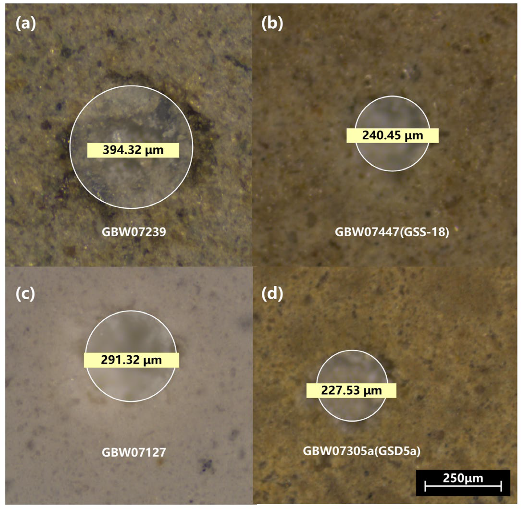
Besides spectra acquisition, we also examined the dimension information of the ablation craters via an optical metallurgical microscope (Leica DM2700 M, Leica Microsystems, Wetzlar, Germany). As shown in Figure 3, the diameters of the craters (after 60 laser shots) can vary from approximately 220 µm to 400 µm, depending on the optical and thermal properties of the materials.

2.3. Spectral Preprocessing

In this work, a series of preprocessing steps were applied to the raw spectral data, including dark subtraction, wavelength calibration and drift correction, invalid pixel screening, and channel splicing. The spectral preprocessing pipeline is expected to improve data quality and hence enhance the accuracy of the quantitative analysis.

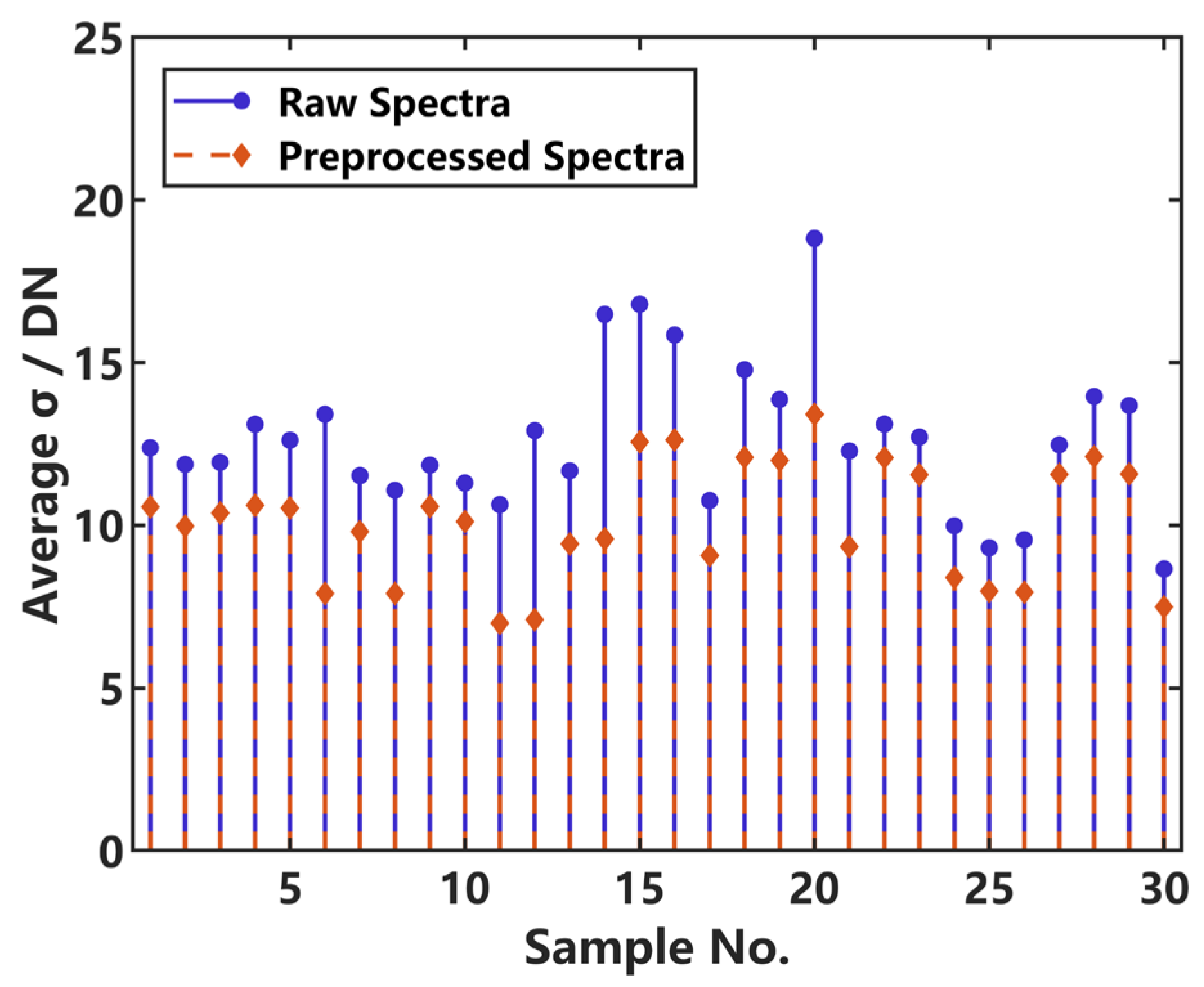
One of the most crucial indices for evaluating the LIBS data quality is spectral reproducibility. In order to validate the effectiveness of the preprocessing, we computed the average standard deviation (σ) of the 60 spectra for each of the 30 target samples. For each sample, we first calculated the standard deviation σ value at each pixel point across the 60 spectra. Since each spectrum consists of 4506 pixel points (with the spectral intensity values represented by a digital number, DN), we could obtain 4506 individual σ values per sample. Then we calculated the average of the 4506 values and acquired the average σ value of each sample. The sample-level average σ value serves as a metric of the shot-to-shot fluctuation, with a lower average σ indicating better spectral reproducibility.

As shown in Figure 4, the average σ value of every sample can more or less decrease after spectral preprocessing, demonstrating the effectiveness of preprocessing in reducing shot-to-shot fluctuation.

Table 3. Statistics of the sample-level average σ values over the 30 samples, including the mean, median, maximum, and minimum, from raw spectra vs. preprocessed spectra.

Spectra Data	Mean	Median	Maximum	Minimum
Raw Spectra	12.65	12.43	18.82	8.66
Preprocessed Spectra	10.11	10.25	13.41	7.00

summarizes the overall statistics of the sample-level average σ values across all 30 target samples. All statistical indicators, including the mean, median, maximum, and minimum, consistently decrease after spectral preprocessing.

These results confirm that the preprocessing work can effectively improve the LIBS data quality, thus providing a solid foundation for promoting the accuracy and reliability of the subsequent quantification results.

2.4. Methods

In this study, we propose a novel LIBS chemometric method, namely BOTS-BPNN, which employs a tunable Softplus function as the hidden layer activation function of the BPNN and utilizes Bayesian optimization to search for the proper tunable hyperparameter β. The overall diagram of the BOTS-BPNN method is exhibited in Figure 5.

As described above, we collected 60 raw LIBS spectra from each of the 30 samples, obtaining a total of 1800 LIBS spectra, and these raw spectra underwent a series of preprocessing steps. Notably, we employed the full data of every LIBS spectrum (comprising 4506 pixel data points) as the input of the BPNN model. In other words, the MgO content is predicted by comprehensively utilizing the entire spectrum rather than a few individual Mg characteristic lines. Such an operation can maximize the utilization of spectral data without missing any valuable information.

To train and test the model, an 80/20 data partition scheme was adopted for the operation of the BOTS-BPNN model. Specifically, 1440 spectra of 24 samples were used as the training set, and 360 spectra of 6 samples were employed as the test set.

The following sections provide more details of the BPNN model with a tunable Softplus activation function and the Bayesian optimization procedure. Additionally, we will briefly introduce the RF method, which has been used for model performance comparison.

2.4.1. Backpropagation Neural Network (BPNN)

Figure 6a illustrates a typical BPNN, which comprises an input layer, a hidden layer, and an output layer. The hidden layer serves as the core computational component, leveraging its activation function to realize complex nonlinear feature mapping between the input and output variables. Common activation functions include Sigmoid, Tanh, ReLU, Softplus (specifically referring to ordinary Softplus), etc. The Sigmoid function, which maps inputs to the (0, 1) range, has historically been widely used in neural networks. However, it suffers from gradient saturation when inputs are large or small, leading to vanishing gradients and reduced training efficiency [39]. Additionally, its non-zero-centered output can slow convergence in gradient-based optimization. The Tanh function, which maps inputs to the (–1, 1) range, addresses the zero-centered issue but still experiences saturation-related problems [40]. The ReLU function mitigates the gradient vanishing phenomenon in the positive domain with a constant gradient, but its zero gradient in the negative domain can lead to the notorious problem of dying neurons. In addition, ReLU and its variants (e.g., PReLU and Leaky ReLU) may suffer from the gradient explosion problem [41]. The ordinary Softplus function provides a smooth and differentiable approximation of ReLU and hence can address the “dead neuron” issue, but its function form is rigid and the model flexibility is low [42].

In the BPNN model, the hidden layer adopts a tunable Softplus (abbreviated as “T-Softplus” hereafter) function as the activation function. While retaining the advantages of the ordinary Softplus function, the T-Softplus function has better flexibility since it introduces a tunable β parameter, as defined by Equation (1).

$$\mathrm{T}\text{-}\mathrm{S}\mathrm{o}\mathrm{f}\mathrm{t}\mathrm{p}\mathrm{l}\mathrm{u}\mathrm{s}\left(x\right)={\displaystyle \frac{1}{\beta }}\mathrm{l}\mathrm{o}\mathrm{g}\left(1+{\mathrm{e}}^{\beta x}\right)$$

(1)

As shown in Figure 6b, different β values can obviously lead to different curvatures of the T-Softplus function. It is noteworthy that when β = 1, the curve corresponds to the ordinary Softplus function. The tunable β value brings high flexibility, thereby enhancing the BOTS-BPNN model’s ability to fit complex patterns and extract nonlinear features. When a proper β parameter is adopted, the model can achieve high quantitative accuracy, as demonstrated in Section 3.

2.4.2. Bayesian Optimization Strategy

Since the β parameter may considerably impact the performance of the BOTS-BPNN model, it is important to search for the optimal β value. While traditional optimization methods such as grid search (GS) and stochastic search are straightforward and easy to implement, they are computationally inefficient, particularly when the parameter space is large and complex. To find a proper parameter value for a certain LIBS dataset, these searching strategies may need to bear extraordinarily high time costs, and the result may not be satisfactory even if a lot of time is spent. In contrast, Bayesian optimization (BO) offers a more efficient approach by constructing a probability distribution of the objective function through a surrogate model, which enables the approximation of the global optimal solution. The BO method allows for automatic searching for the optimal parameter and only needs a few search iterations.

In this work, the specific scheme used to implement BO is the tree-structured Parzen estimator (TPE), which can leverage non-parametric density estimation via Parzen windows to model the parameter-searching space. The TPE scheme is suitable for hyperparameter optimization in ANN-type models, supporting mixed variable types, including categorical (e.g., activation function type), discrete (e.g., kernel size), and continuous (e.g., learning rate) parameters [43].

TPE constructs two separate probability density models: one for hyperparameter configurations associated with good-performance outcomes, and the other for those associated with poor-performance outcomes. As described in Equations (2) and (3), β represents the hyperparameter to be optimized, while γ is the threshold used to distinguish between good and poor performance. The conditional probability density functions l(β) and g(β), constructed via kernel density estimation under the assumption of independence among hyperparameters, characterize the distribution of β in the good- and poor-performance regions in the whole hyperparameter space B, respectively.

$$l\left(\beta \right)=p\left(\beta \mid f\left(\beta \right)\le \gamma \right)$$

(2)

$$g\left(\beta \right)=p\left(\beta \mid f\left(\beta \right)>\gamma \right)$$

(3)

Based on a random initial trial hyperparameter value, the TPE algorithm selects the next trial value by maximizing the so-called expected improvement (EI), as described in Equations (4) and (5). By iteratively updating, the hyperparameter efficiently converges toward the optimal value.

$$\mathrm{E}\mathrm{I}\left(\beta \right)={\displaystyle \frac{p\left(\beta \mid f\left(\beta \right)\le \gamma \right)}{p\left(\beta \mid f\left(\beta \right)>\gamma \right)}}$$

(4)

$${\beta }_{new}=arg\underset{\beta \in \mathcal{B}}{max}\mathrm{E}\mathrm{I}\left(\beta \right)$$

(5)

In this study, both the TPE-based BO method and the traditional GS method have been adopted to search for the proper β parameter for the BPNN model’s T-Softplus activation function. The BPNN model performance comparison between the two searching methods is displayed in Section 3.

2.4.3. Random Forest (RF)

Besides investigating the BPNN model, this work has also introduced RF as an alternative model for performance comparison. The RF method constructs an ensemble of weak learners—typically decision trees—and aggregates their outputs through majority voting or averaging. Its predictive strength relies on two core techniques, bootstrap aggregation (bagging) and random feature selection, which jointly improve generalization and mitigate the overfitting typically observed in individual decision trees. These mechanisms also contribute to RF’s advantages in modeling efficiency and overfitting control, making it a popular LIBS chemometric method [44].

3. Results

3.1. Model Performance on Test Set

In order to assess the predictive performance of the proposed BOTS-BPNN model on the LIBS dataset, we calculated two metrics from the testing set samples, i.e., root mean square error (RMSE) and relative error (RE), as defined by Equations (6) and (7), respectively.

$$\mathrm{R}\mathrm{M}\mathrm{S}\mathrm{E}=\sqrt{{\displaystyle \frac{1}{n}}\sum _{i=1}^n{\left(y_i-{\widehat{y}}_i\right)}^2}$$

(6)

$$\mathrm{R}\mathrm{E}={\displaystyle \frac{1}{n}}\sum _{i=1}^n{\displaystyle \frac{\left|y_i-{\widehat{y}}_i\right|}{y_i}}\times 100\mathrm{\%}$$

(7)

Here n represents the total number of spectra for the given test sample, y_i represents the real concentration value corresponding to the i-th spectrum, and ŷ_i denotes the predicted concentration value for that spectrum.

3.2. BOTS-BPNN Prediction Accuracy and Confidence Interval Analysis

As mentioned before, there are six testing set samples (corresponding to 360 LIBS spectra) in this study. The six testing samples are andesite (GBW07104(GSR-2)), lead ore type-I (GBW07235), copper-rich ore (GBW07164(GSO-3)), argillaceous limestone (GBW07108(GSR-6)), polymetallic lean ore (GBW07162(GSO-1)), and stream sediment type-II (GBW07377(GSD-26)). And they are denoted as Test Sample 1, Test Sample 2, … and Test Sample 6, respectively.

The prediction accuracy of the BOTS-BPNN model is evaluated by the RMSE and RE values on the testing set, as displayed in

Table 4. RMSE and RE values obtained by the BOTS-BPNN model on the testing samples.

Test Sample No.	RMSE (wt.%)	RE (%)
1	0.2829	14.19
2	0.3279	16.67
3	0.3524	12.84
4	1.1794	18.72
5	0.1648	7.67
6	0.4140	21.28
Average	0.4536	15.35

. These results are achieved based on the optimal β value (denoted as β_opt) obtained by the BO method, and β_opt = 8.35 here.

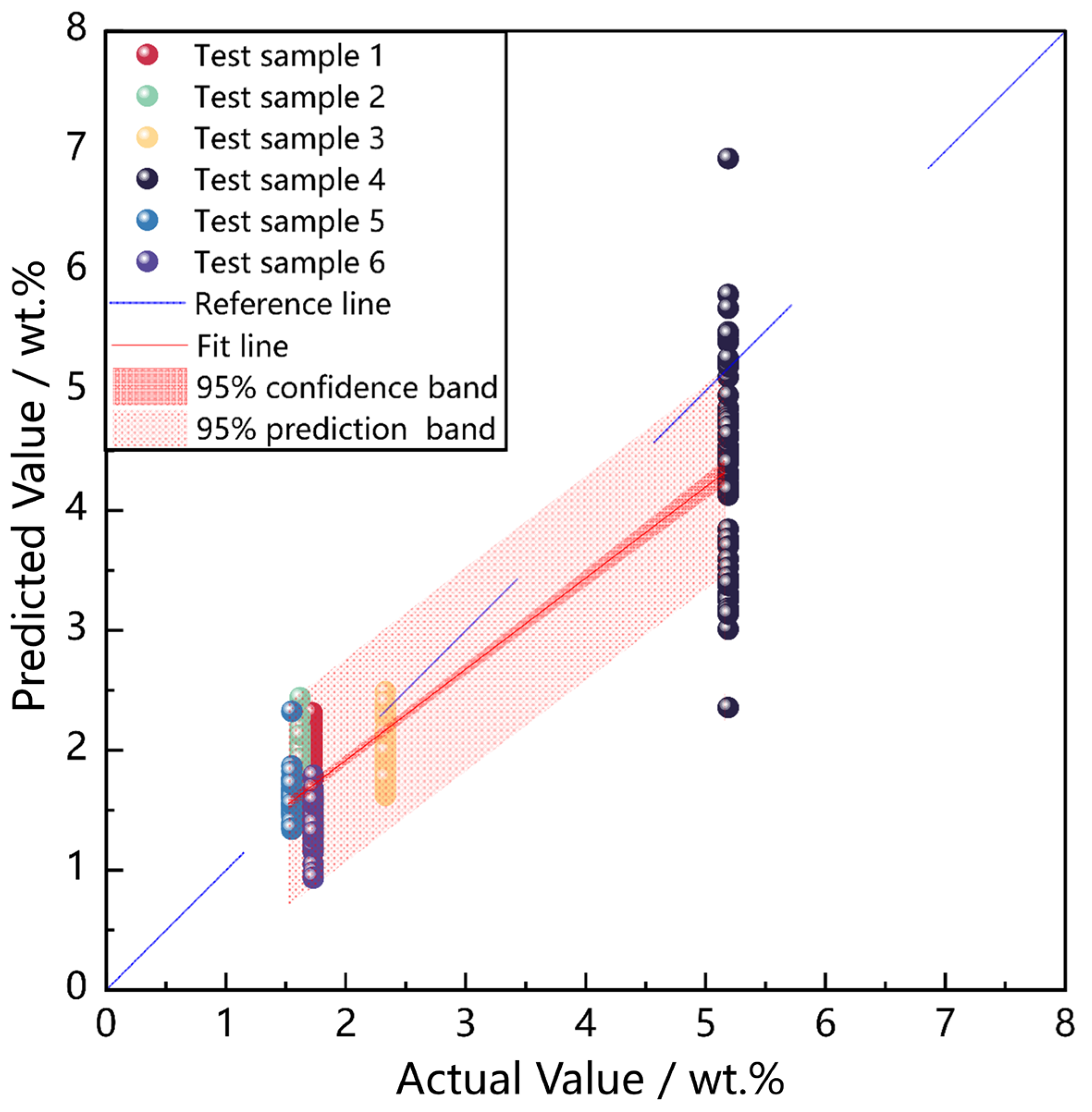
Figure 7 presents the regression results for six test samples, each comprising 60 independent LIBS spectra. The blue dashed line denotes the ideal y = x reference line, while the red solid line represents the model’s fitted regression line. The dark-red-shaded area indicates the 95% confidence interval, while the light-red-shaded area represents the 95% prediction interval. Both were calculated based on the linear regression between actual and predicted values across all test samples, using the residual standard error and the t-distribution to estimate uncertainty in the fitted mean response and the expected range of individual predictions, respectively.

The 95% confidence interval provides a range of values within which we can be 95% confident that the true regression line lies. The light-red-shaded area represents the prediction interval, which indicates the expected range of future individual predictions for new data points. Each scatter marker corresponds to one of the six test samples. The confidence and prediction intervals offer valuable insights into the uncertainty of the model’s predictions and its ability to generalize to new data, thereby enhancing the reliability and robustness of the quantitative analysis.

As presented in Figure 7, for most of the test samples, the predicted MgO concentration values are tightly clustered around the reference line, indicating high prediction accuracy. Additionally, the majority of predictions fall within the 95% confidence interval, showcasing the robustness of the BOTS-BPNN model. However, noticeable deviations can be observed in Test Sample 4, with quite a few predictions falling outside the light red 95% prediction interval.

This is attributed to the fact that Test Sample 4 has a significantly higher MgO concentration than most of the target samples. As mentioned in Section 2.2, the MgO concentration values in most samples are less than 2 wt.%. Due to the lack of high-MgO-concentration samples in the training set, the model’s prediction accuracy and stability in the high-concentration region are not so good. Despite the relatively low performance for this particular sample, the BOTS-BPNN model generally behaves well on the testing sample set, demonstrating its potential for complicated LIBS quantitative analysis.

3.3. Search Method Comparison

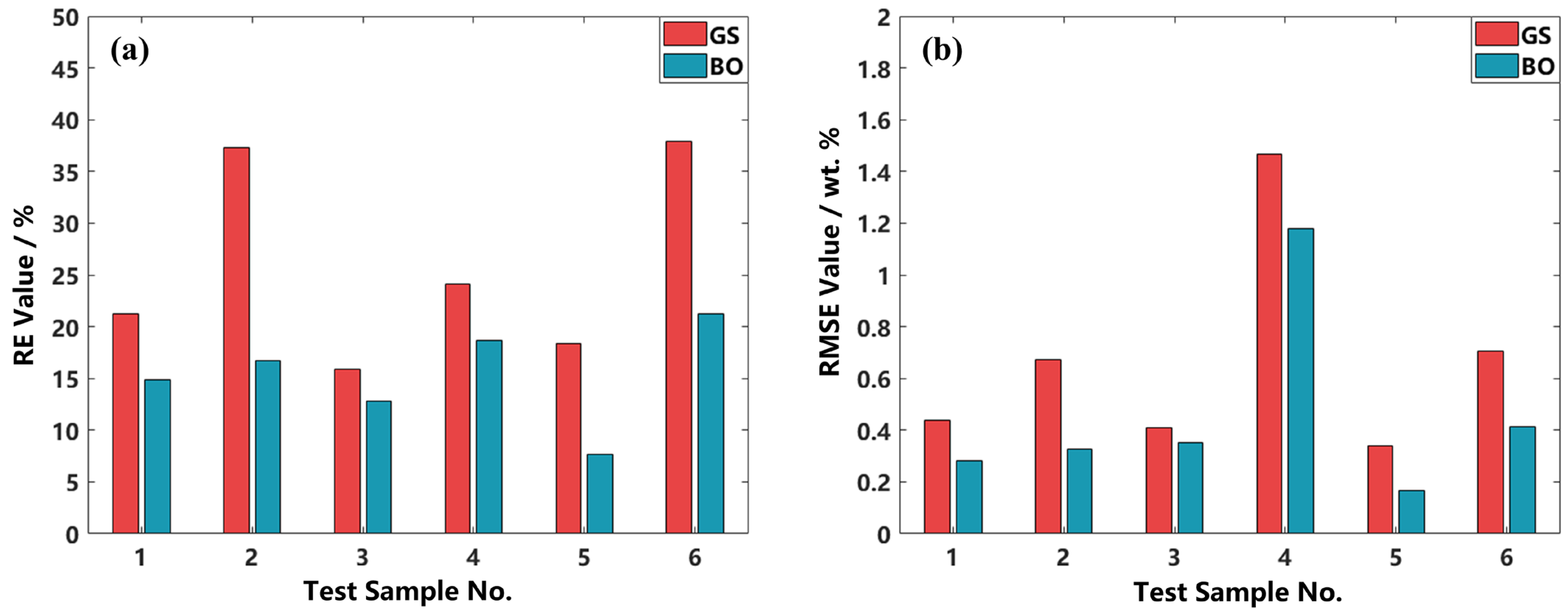
The above results were achieved on the basis of the TPE-based BO searching method. To demonstrate its superiority, we compare the error levels of the BO method with those of the traditional GS method, as illustrated in Figure 8a (RE values) and Figure 8b (RMSE values), respectively.

Based on the RE and RMSE results, it is evident that the BO method is superior to the traditional GS method since it yields both lower RE values and lower RMSE values on all the test samples. Specifically, the mean RE value of the BO method is 15.35%, while that of the GS method is 25.79%, and the mean RMSE value of the BO method is 0.4536 wt.%, while that of the GS method is 0.6723 wt.%. Statistical analysis further indicates that the standard deviation of RE obtained using BO is 4.35%, markedly lower than the 8.71% observed with GS. The lower standard deviation implies the better stability and robustness of the BO search method.

Notably, the performance gap between BO and GS is substantially reduced for Test Sample 3, with the corresponding differences in RE and RMSE being markedly smaller than those observed for the other samples. This is likely due to the dense representation of this concentration range in the training set, allowing the model to achieve good accuracy regardless of the tuning method. This suggests that when the training data sufficiently cover the target concentration range, model performance may become less sensitive to hyperparameter tuning, with the dominant influence potentially shifting to the intrinsic architecture design.

Beyond predictive accuracy, BO offers notable advantages in terms of computational efficiency and convergence speed. While GS exhaustively explores the discrete parameter space, it remains inefficient even when optimizing a single hyperparameter, as it requires evaluating a broad range of potential values. In contrast, BO constructs a surrogate probabilistic model and uses an acquisition function to dynamically guide the search process, allowing it to identify the optimal parameter with fewer iterations. This approach improves optimization efficiency, as previously demonstrated [43].

In summary, BO demonstrates superior convergence efficiency and enhanced predictive reliability when modeling high-dimensional LIBS spectra. By framing hyperparameter tuning as a probabilistic optimization task, BO improves model performance without increasing structural complexity. This approach is particularly well-suited for LIBS applications involving wide concentration ranges and complex spectral noise. The results further underscore the critical role of both the optimization strategy and training data distribution in defining the upper limits of model performance.

3.4. Robustness Validation of BOTS-BPNN Model

Besides accuracy, robustness is also a critical factor for evaluating model performance in real-world applications. Therefore, we have inspected the robustness of the BOTS-BPNN model from three aspects.

Firstly, the model’s sensitivity to perturbations in the key hyperparameter β is explored. To be more specific, the sensitivity is assessed by introducing minor variations (±0.001) to the optimized value of β (all other parameters, e.g., network architecture and training protocol, remain identical to the main experiments).

As shown in

Table 5. Comparison of BOTS-BPNN model performance under perturbations around the optimized β value β_opt (β_opt − 0.001/β_opt/β_opt + 0.001). The model performance is evaluated by the RMSE value (wt.%) on the six test samples.

Test Sample No.	RMSE (βopt − 0.001)	RMSE (βopt)	RMSE (βopt + 0.001)
1	0.3012	0.2829	0.3074
2	0.3511	0.3279	0.3567
3	0.3683	0.3524	0.3692
4	1.3144	1.1794	1.1821
5	0.1748	0.1648	0.1663
6	0.4378	0.4140	0.4207
Average	0.4913	0.4536	0.4671

, minor variations are observed in the RMSE values under perturbations around the optimized β value, and the overall prediction performance remains largely consistent. These small fluctuations suggest that the model’s predictive performance is relatively stable with respect to small changes in this key hyperparameter.

Secondly, the model robustness is examined from the perspective of input data, including two aspects, namely, information loss and random noise.

Regarding information loss, we fabricated partial loss by randomly removing two, four, and six spectra from the training set. Apart from the reduced training set size, all other parameters remain unchanged.

As shown in

Table 6. Comparison of the BOTS-BPNN model performance under different training set conditions (0/2/4/6 spectra randomly removed). The model performance is evaluated by the RMSE value (wt.%) on the six test samples.

Test Sample No.	RMSE (0 rmv)	RMSE (2 rmv)	RMSE (4 rmv)	RMSE (6 rmv)
1	0.2829	0.2972	0.3136	0.3307
2	0.3279	0.3810	0.3680	0.3408
3	0.3524	0.3462	0.3497	0.3760
4	1.1794	1.1936	1.1998	1.2006
5	0.1648	0.1687	0.1784	0.1837
6	0.4140	0.4256	0.4446	0.4555
Average	0.4536	0.4687	0.4757	0.4812

, the overall trend exhibits a slight rise in RMSE values with the increasing number of removed training spectra. However, the performance degradation is within a rather limited range. This observation suggests that the model can maintain a relatively stable performance when training set information is partially lost.

As for random noise, we designed three groups of Gaussian noise perturbation examinations. Specifically, in each examination, six spectra are randomly selected from the training set and subjected to additive Gaussian noise. For each spectrum, the introduced Gaussian noise data has a zero mean and a standard deviation set to 0.5% of the maximum intensity value within the spectrum. Aside from the difference in the specific selected spectra, the three groups of examinations are identical in terms of the noise model, number of perturbed spectra, and training strategy. The results of these noise-perturbed examinations are compared with those obtained under the baseline condition in which no noise is added, as summarized in

Table 7. Comparison of BOTS-BPNN model performance with and without Gaussian random noise added to the training set spectra (no noise/noise group 1/noise group 2/noise group 3). The model performance is evaluated by the RMSE values (wt.%) on the six test samples.

Test Sample No.	RMSE (No Noise)	RMSE (Noise 1)	RMSE (Noise 2)	RMSE (Noise 3)
1	0.2829	0.3183	0.3013	0.3107
2	0.3279	0.3603	0.3502	0.3511
3	0.3524	0.3602	0.3721	0.3601
4	1.1794	1.2241	1.2644	1.2418
5	0.1648	0.1632	0.1784	0.1601
6	0.4140	0.4465	0.4514	0.4455
Average	0.4536	0.4788	0.4863	0.4782

.

The model exhibits relatively consistent performance in the presence of noise, suggesting that it is able to withstand a certain level of random noise in the training spectra.

Building upon the training set noise perturbation examinations, we further introduce the same type of Gaussian noise into the test set. Specifically, six spectra are randomly selected from the test set and subjected to noise perturbation, simulating potential fluctuations in spectral quality during field detection. The results of the test set noise examinations are displayed in

Table 8. Comparison of the BOTS-BPNN model with and without Gaussian random noise added to the test set spectra. The model performance is evaluated by the RMSE values (wt.%) on the six test samples.

Test Sample No.	RMSE (No Noise)	RMSE (With Noise)
1	0.2829	0.3058
2	0.3279	0.3809
3	0.3524	0.2876
4	1.1794	1.8615
5	0.1648	0.1792
6	0.4140	0.4447
Average	0.4536	0.5766

.

Generally speaking, the model performance does not significantly decay when the test spectra are perturbed by random noise. However, one exception is observed for Test Sample 4, with the RMSE value noticeably rising under the noise. This might be due to the sample’s inherent large spectral variability and the high noise amplitude, and the exact reason needs to be further investigated.

The three aspects of examinations mentioned above suggest that the BOTS-BPNN model can withstand a certain level of perturbations in model hyperparameters and input data, and hence, the model robustness has been validated to some extent.

3.5. Comparative Analysis of BOTS-BPNN and Traditional BPNN Models with Classical Activation Functions

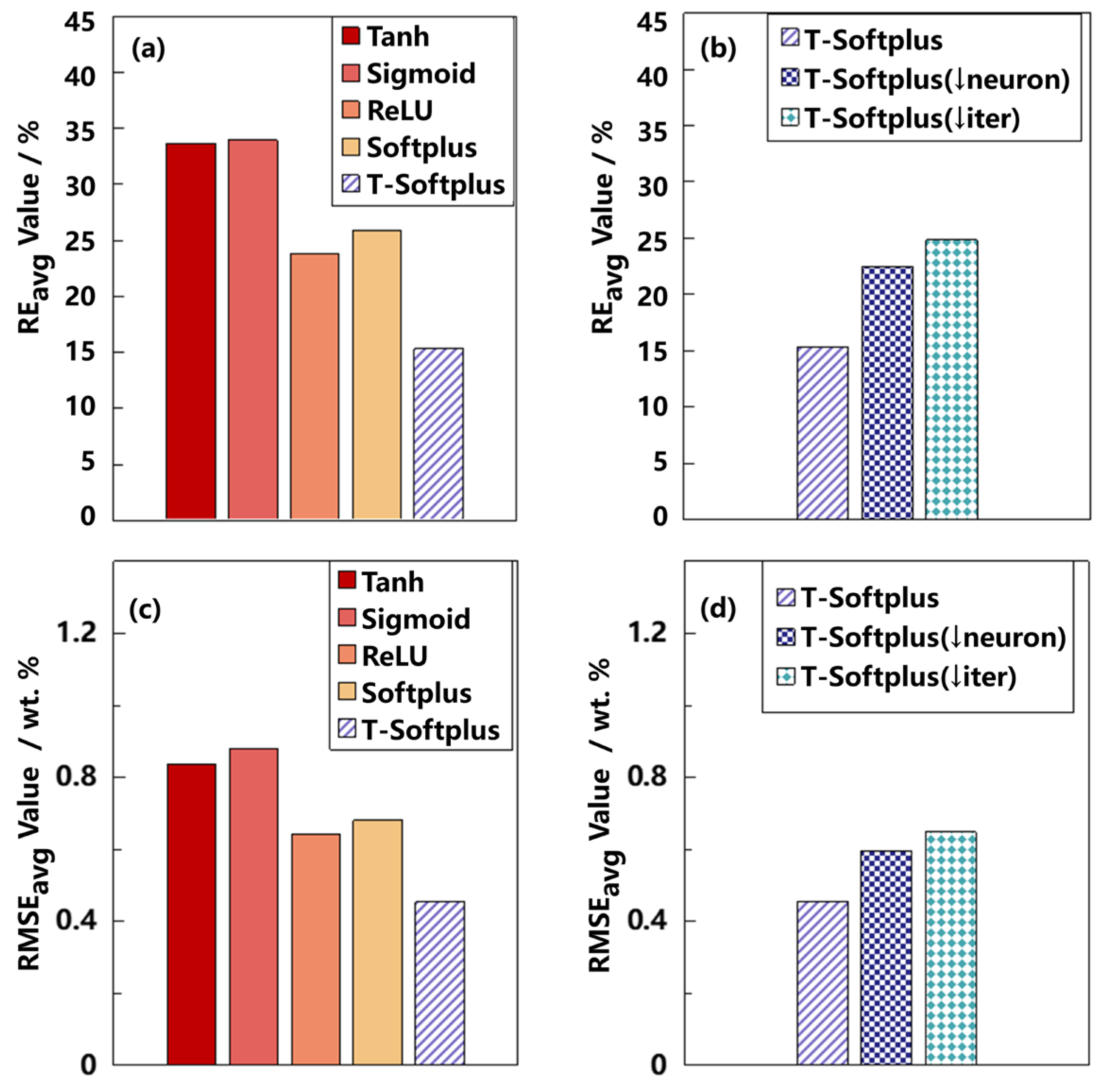
To systematically evaluate the impact of activation functions on the performance of BPNN models in LIBS-based quantitative analysis, we compared five activation functions—Tanh, Sigmoid, ReLU, Softplus, and T-Softplus—under identical network configurations.

Table 9. Performance comparison of different activation functions (bold: best; underlined: second best).

Test Sample No.	Activation Function	RMSE (wt.%)	RE (%)
1	Tanh	0.4735	21.18
	Sigmoid	0.4182	22.25
	ReLU	0.4106	19.28
	Softplus	0.5385	25.01
	T-Softplus	0.2829	14.91
2	Tanh	1.1017	64.18
	Sigmoid	0.7725	44.86
	ReLU	0.7185	40.58
	Softplus	0.8046	45.83
	T-Softplus	0.3279	16.67
3	Tanh	0.8760	36.34
	Sigmoid	1.1234	48.05
	ReLU	0.3683	13.67
	Softplus	0.5023	20.09
	T-Softplus	0.3524	12.84
4	Tanh	1.6031	29.09
	Sigmoid	2.1063	40.38
	ReLU	1.5146	25.22
	Softplus	1.5410	28.01
	T-Softplus	1.1794	18.72
5	Tanh	0.2570	13.83
	Sigmoid	0.2656	15.10
	ReLU	0.2443	13.10
	Softplus	0.2098	10.32
	T-Softplus	0.1648	7.67
6	Tanh	0.6951	37.19
	Sigmoid	0.5972	33.15
	ReLU	0.5923	31.00
	Softplus	0.4884	25.82
	T-Softplus	0.4536	21.28

presents the RMSE and RE values obtained for MgO concentration predictions on the test set. For clarity, the best and second-best values of each metric are highlighted in bold and underlined, respectively.

The results show that the model employing the T-Softplus activation function consistently achieves the lowest RMSE across the test set, with marked advantages in samples 1, 2, 4, and 5. In terms of RE, T-Softplus also outperforms all other functions. For instance, in Sample 2, it reduces RE from 64.18% (using Tanh) to just 16.67%; similarly, for Sample 3, RE drops from 48.05% (using Sigmoid) to 12.84%, reflecting the model’s superior accuracy and stability.

While ReLU and Softplus show competitive performance in specific cases (e.g., Samples 2 and 6), they fail to match the overall accuracy and robustness of T-Softplus. In contrast, Tanh and Sigmoid yield significantly higher RMSE and RE values, with greater variability across samples. Tanh, for example, produces RE values ranging from 13.83% to 64.18%, while Sigmoid ranges from 15.10% to 48.05%. Their standard deviations in RE are 15.92% and 11.92%, respectively—substantially higher than the 4.99% observed with T-Softplus.

These findings suggest that T-Softplus provides better adaptability for capturing the nonlinear spectral features inherent in LIBS data. Even when trained on limited or unevenly distributed datasets, it maintains strong predictive performance and stability across samples. Its tunable parameter β enables dynamic adjustment of the activation curve shape, improving model expressiveness without increasing structural complexity.

3.6. Comparative Performance Evaluation of BOTS-BPNN and RF for LIBS Quantification

In addition to evaluating the influence of activation functions, we compared the proposed BOTS-BPNN model with the traditional RF algorithm to assess its relative performance in LIBS-based elemental analysis. The results for all evaluation metrics are summarized in

Table 10. Performance comparison of RF model with BOTS-BPNN model.

Test Sample No.	Model	RMSE (wt.%)	RE (%)
1	RF	0.3046	16.09
	BOTS-BPNN	0.2829	14.91
2	RF	0.3243	19.76
	BOTS-BPNN	0.3279	16.67
3	RF	0.4964	18.56
	BOTS-BPNN	0.3524	12.84
4	RF	2.1094	37.30
	BOTS-BPNN	1.1794	18.72
5	RF	0.4027	21.60
	BOTS-BPNN	0.1648	7.67
6	RF	0.5007	27.70
	BOTS-BPNN	0.4140	21.28

.

For test samples 1, 2, and 3, although the BOTS-BPNN model does not show a pronounced reduction in RMSE compared to the RF model, it achieves significantly lower RE. For Test Samples 4, 5, and 6, the BOTS-BPNN model outperforms RF in both RMSE and RE, indicating stronger predictive accuracy and robustness across a broader range of concentrations.

These results reflect fundamental differences in the feature learning capabilities of the two models. RF, as an ensemble method, has limited capacity to model complex nonlinear interactions among high-dimensional spectral features. Its decision-tree-based partitioning strategy may restrict its expressiveness when dealing with subtle spectral variations. In contrast, the BOTS-BPNN model—built upon a backpropagation neural network enhanced with the tunable T-Softplus activation function—demonstrates superior adaptability in extracting nonlinear and latent patterns from LIBS spectra. This leads to improved quantitative prediction across diverse test conditions.

Notably, the enhanced RE performance of BOTS-BPNN suggests superior generalization in low-concentration samples, a critical capability in practical LIBS applications where detecting trace elements is often required. Precise modeling of small concentration fluctuations is essential for accurate elemental quantification under Martian conditions.

In summary, the BOTS-BPNN model not only surpasses the RF model in overall prediction accuracy but also offers greater interpretability and generalization, making it well-suited for LIBS-based quantitative analysis of complex, high-dimensional, and imbalanced datasets.

4. Discussion

Beyond the results presented in Section 3, this section further discusses the underlying superiority of the proposed BOTS-BPNN model and the potential generalization scenarios of the BOTS-BPNN method.

4.1. The Underlying Superiority of the BOTS-BPNN Model

Having demonstrated that the T-Softplus activation function outperforms conventional activation functions in the standard BPNN configuration, we further show the underlying superiority of the BOTS-BPNN model, i.e., its high performance even when the number of hidden layer neurons or the number of training epochs is considerably reduced.

To be more specific, in the standard BPNN configuration described in Section 2, the number of hidden layer neurons and the number of training epochs are 100 and 250, respectively (identical for all the activation functions), while herein, two new BPNN models (with T-Softplus activation function) have been tried, one with only 50 neurons (still 250 epochs), and the other with only 125 epochs (still 100 neurons).

Figure 9a compares the RE_avg values for the five activation functions in the full network configuration (100 hidden layer neurons and 250 training epochs). Figure 9b compares the RE_avg values for the two BPNN models (with T-Softplus activation), one using 50 neurons (250 epochs) and the other using 125 epochs (100 neurons). Figure 9c compares the RMSE_avg values for the five activation functions in the full network configuration (100 hidden layer neurons and 250 training epochs). Figure 9d compares the RMSE_avg values for the two BPNN models (with T-Softplus activation), one using 50 neurons (250 epochs) and the other using 125 epochs (100 neurons).

Figure 9 demonstrates that the BPNN model with the T-Softplus activation function performs optimally in the full network configuration (100 hidden layer neurons and 250 training epochs), achieving the lowest RE_avg and RMSE_avg values (see Figure 9a,c). As the model complexity decreases, with BPNN models using T-Softplus activation—one with only 50 neurons (maintaining 250 epochs), and the other with only 125 epochs (maintaining 100 neurons)—the RE_avg and RMSE_avg values slightly increase (see Figure 9b,d), though these changes are modest and acceptable. Even with a reduction in the number of neurons and training epochs, T-Softplus still outperforms Tanh and Sigmoid in terms of quantitative performance. In comparison with the full network configurations using ReLU and Softplus, T-Softplus provides slightly better quantitative results with fewer neurons, and comparable results in terms of the overall network configuration when fewer epochs are used.

These findings highlight that T-Softplus provides a better balance between modeling capability and computational complexity. Its adaptive β parameter allows the activation curve to dynamically adjust according to the distribution of training samples. This enhances the network’s ability to capture high-dimensional sparsity and local nonlinearities, even in more compressed architectures. Furthermore, the results confirm that T-Softplus offers strong robustness and predictive reliability while reducing computational requirements. This makes it especially valuable for field applications like Mars exploration, where efficiency and the model’s ability to flexibly adapt to harsh planetary environments are crucial. The BOTS-BPNN model, with its adaptive activation mechanism, provides a balanced solution between performance and resource constraints, serving as a reference framework for LIBS chemometrics in planetary missions.

4.2. Future Prospects

The BOTS-BPNN method is expected to be generalized in several aspects, as discussed below.

• Although the superiority of the T-Softplus activation function has been validated within a BPNN framework in this work, its strong nonlinearity fitting ability and high adaptability are expected to be generalized to other ANN architectures, such as the CNN, another popular algorithm in LIBS studies [45,46]. Embedding the T-Softplus activation function in convolutional layers and/or dense layers might improve the CNN’s prediction performance without adding to the number of layers of the model.
• The LIBS detection distance in this experiment was maintained at a fixed value, namely, 2 m. In Mars field detection, however, the LIBS detection distance would naturally vary from time to time. It is necessary to analyze a dataset consisting of multi-distance mixed spectra, which can be a challenging task for both classification and quantification. The BOTS-BPNN method is expected to analyze not only uni-distance spectra but also multi-distance spectra. This may be effective especially when the T-Softplus activation function is adopted in a CNN model, since previous work has demonstrated that a CNN is a powerful chemometric method for tackling multi-distance LIBS spectra [47].
• In this work, all the target samples were placed in a vacuum cabin and had clean surfaces. But in the real in situ detection on Mars, the target samples are prone to being contaminated on their surfaces by Martian dust. Among the LIBS spectra collected from a certain target sample, some of them may be the spectra of the surface dust rather than those of the underlying actual sample. Since the BPNN can perform both qualitative and quantitative analysis, the BOTS-BPNN method can be utilized in two aspects. On the one hand, it may benefit data identification, distinguishing the actual-sample spectra from the surface-dust spectra. On the other hand, based on the selected actual-sample spectra, the BOTS-BPNN method may help to improve the accuracy of the subsequent concentration quantification, just like the analysis shown in this research.
• Besides the Martian dust problem, the environment on Mars can differ from that of an Earth laboratory in many other aspects, such as the gas composition, pressure, and temperature. The environmental differences can lead to considerable discrepancies in LIBS spectra profiles, even for the same target sample. The spectral discrepancies can make the chemometric model trained on Earth laboratory data ineffective when analyzing Mars in situ data. To address this issue, we have proposed a novel methodology based on transfer learning in one of our recent studies, with the specific pattern being pretrained-model-based transfer learning and the pretrained model being a CNN [48]. The effectiveness of this methodology has been demonstrated on the ChemCam dataset. It is worth emphasizing that this methodology may not focus on the discrepancy caused by any one specific factor (e.g., environment), but is oriented to the overall discrepancy effect caused by all the relevant factors. By the way, there has been work focusing on the spectral discrepancy caused by matrix effects, which include chemical matrix effects (the spectral features influenced by chemical properties of the sample matrix) and physical effects (the spectral features influenced by physical properties of the sample matrix). For instance, a method to address the issues of physical effects has been reported in [49]. The method is also based on transfer learning, but the specific patterns are instance-based transfer learning and feature-based transfer learning. In our future research, more transfer-learning-based schemes will be developed. The BOTS-BPNN may serve as a pretrained model if the pretrained-model-based pattern is adopted, and may serve as a feature extraction tool if the feature-based pattern is adopted. Moreover, we will enlarge the training dataset by introducing samples that span a far broader spectrum of chemical and physical properties—for example, adding diverse lithologies such as evaporitic and hydrothermally altered rocks, as well as various soils, ores, and sediment types. Physically, we will cover a controlled range of surface roughnesses, particle size distributions, moisture contents, and porosities or compaction states. This systematic diversification is expected to enhance model generalizability across heterogeneous planetary and terrestrial scenarios.
• Nowadays a development trend of LIBS analysis is to integrate LIBS spectra and other relevant physical parameters as the input of the chemometrics model, e.g., the plasma temperature and density, the images of plasma, the images of laser ablation crater, etc. [50,51]. It is expected that the additional physical parameter data can help the BOTS-BPNN model extract more useful features. Other ways to leverage physical knowledge include embedding physical constraints (e.g., plasma dynamics) into the neural network, usually called a physics-informed neural network (PINN) [52], and integrating physical descriptors (e.g., electron density gradients and temperature decay rates) as optimization objectives [53]. The designed BOTS-BPNN model may also be generalized to such a physics-informed methodology.

The potential generalization scenarios of the BOTS-BPNN method proposed in this study imply that this method may practically contribute to the analysis of Mars in situ LIBS data.

5. Conclusions

In this study, we have proposed a novel BOTS-BPNN method for LIBS quantitative analysis. The experimental dataset comprises 1800 LIBS spectra collected from 30 geochemical samples by a MarSCoDe laboratory duplicate in a Mars-simulated environment. The MgO component has been taken as an example for concentration quantification.

To ensure the spectral data quality, a series of spectral preprocessing steps have been carried out. This preprocessing work has been demonstrated to enhance shot-to-shot spectral reproducibility, thereby helping improve the accuracy and reliability of the subsequent quantitative analysis.

With the LIBS dataset, the BOTS-BPNN model can exhibit better accuracy performance than BPNN models employing conventional activation functions (e.g., Tanh, Sigmoid, ReLU, and ordinary Softplus), as long as the proper β parameter is adopted in the T-Softplus function. The BOTS-BPNN model can also surpass other popular machine learning algorithms, such as the RF algorithm.

Moreover, the proposed BOTS-BPNN model has the potential to perform well with a simplified version. Specifically, when a reduced number of hidden layer neurons or a reduced number of training epochs is used in the BOTS-BPNN model, it can still demonstrate superiority over BPNN models with conventional activation functions, although the superiority gap will be a bit narrower. Therefore, one of the underlying advantages of the BOTS-BPNN method is its effectiveness under limited computing resources. For the T-Softplus function, besides the accuracy aspect, this work has also inspected the efficiency of the β-searching process. Compared with the traditional GS method, the proposed TPE-based BO method can find the proper β parameter in a significantly more efficient way.

Furthermore, model performance examinations under different perturbation conditions (including hyperparameter alteration, information loss, and random noise) demonstrate the good robustness of the BOTS-BPNN model. This highlights its reliability in field detection, demonstrating its applicability to in situ LIBS analysis in planetary exploration missions.

The results in this study indicate the effectiveness of the proposed BOTS-BPNN model for LIBS analysis. In future work, this methodology may be generalized to other ANN algorithms, like the CNN and PINN, and be utilized to address the challenging issues associated with Mars in situ LIBS detection, such as the varying-distance effect, the surface-dust effect, environmental effects, chemical/physical matrix effects, etc. Since this research has adopted a MarSCoDe duplicate instrument and a Mars-simulated environment, the achievements of this work are expected to offer technical support for analyzing in situ LIBS data from Mars exploration and other planetary exploration missions in the future.