Correction of ASCAT, ESA–CCI, and SMAP Soil Moisture Products Using the Multi-Source Long Short-Term Memory (MLSTM)

Abstract

The Advanced Scatterometer (ASCAT), Soil Moisture Active Passive (SMAP), and European Space Agency-Climate Change Initiative (ESA–CCI) soil moisture (SM) products are widely used in agricultural drought monitoring, water resource management, and climate analysis applications. However, the performance of these SM products varies significantly across regions and environmental conditions, due to in sensor characteristics, retrieval algorithms, and the lack of localized calibration. This study proposes a multi-source long short-term memory (MLSTM) for improving ASCAT, ESA–CCI, and SMAP SM products by combining in-situ SM measurements and four key auxiliary variables: precipitation (PRE), land surface temperature (LST), fractional vegetation cover (FVC), and evapotranspiration (ET). First, the in-situ measured data from four in-situ observation networks were corrected using the LSTM method to match the grid sizes of ASCAT (0.1°), ESA–CCI (0.25°), and SMAP (0.1°) SM products. The RPE, LST, FVC, and ET were used as inputs to the LSTM to obtain loss data against in-situ SM measurements. Second, the ASCAT, ESA–CCI, and SMAP SM datasets were used as inputs to the LSTM to generate loss data, which were subsequently corrected using LSTM-derived loss data based on in-situ SM measurements. When the mean squared error (MSE) loss values were minimized, the improvement for ASCAT, ESA–CCI, and SMAP products was considered the best. Finally, the improved ASCAT, ESA–CCI, and SMAP were produced and evaluated by the correlation coefficient (R), root mean square error (RMSE), and standard deviation (SD). The results showed that the RMSE values of the improved ASCAT, ESA–CCI, and SMAP products against the corrected in-situ SM data in the OZNET network were lower, i.e., 0.014 cm³/cm³, 0.019 cm³/cm³, and 0.034 cm³/cm³, respectively. Compared with the ESA–CCI and SMAP products, the ASCAT product was greatly improved, e.g., in the SNOTEL network, the Root Mean-Square Deviation (RMSD) values of 0.1049 cm³/cm³ (ASCAT) and 0.0662 cm³/cm³ (improved ASCAT). Overall, the MLSTM-based algorithm has the potential to improve the global satellite SM product.

1. Introduction

SM is a critical variable in the terrestrial hydrological cycle [1]. It holds significant importance not only for agricultural production and ecosystem management but also plays an indispensable role in climate change research [2]. Currently, active/passive microwave satellite remote sensing monitoring technology is increasingly applied to SM monitoring at regional and even global scales because of its higher penetration capability compared to optical remote sensing.

Over the past decades, numerous earth observation active/passive microwave satellites have been launched. Based on active/passive microwave SM retrieval algorithms, a variety of microwave satellite SM products have been developed [3,4]. Examples include the ASCAT active microwave SM product using the SWI (Soil Water Index) SM retrieval algorithm [3,4], the AMSR-E (Advanced Microwave Scanning Radiometer for Earth Observation System), the SMAP passive microwave SM product using the LPRM (Land Parameter Retrieval Model), and the SCA-V (Single Channel Algorithm–Vertical polarization) SM retrieval algorithms. The ESA–CCI merged SM products by combining active and passive microwave satellite observations [5,6]. With the development of satellite SM products, many evaluation studies of satellite SM products were conducted through comparisons with in-situ networks, other remote sensing retrievals, or model-based products [7,8,9,10,11,12]. Xu et al. (2021) [13] found that the SMAP product had the highest median R and the lowest median RMSE with in-situ SM measurements in North America using the SM evaluation algorithm based on station data. Zhang et al. (2015) [14] demonstrated that ASCAT can effectively characterize drought conditions across different stations. Moreover, ASCAT showed superior performance in densely vegetated areas compared to products like SMAP [15]. Dorigo et al. (2015) [6] found that ESA–CCI was superior to other single satellite input SM products, e.g., the LPRM-based AMSR-E SM product, particularly in densely vegetated areas. Although some research has shown that the ASCAT, ESA–CCI, and SMAP SM products perform well in arid or semi-arid areas, the accuracy of these satellite SM products varies significantly across different regions due to multiple factors such as sensor band limitations, surface heterogeneity, vegetation water content (VWC), and surface cover types [16,17]. In low vegetation coverage areas, SMAP performs the best, while in high vegetation areas, ASCAT performs even better [15]. In comparisons of overall accuracy and temporal and spatial coverage, the ESA–CCI fused SM product performs best. This shows the advantages of multi-source data fusion in further improving global satellite SM products [16,17].

Many researchers have investigated the influencing factors (e.g., vegetation, land cover, evapotranspiration, etc.) on satellite SM retrieval [18]. Meng et al. (2017) [19] evaluated the consistency between the ESA–CCI SM product and observed precipitation in the Tibetan Plateau area. They found that the positive anomaly in ESA–CCI SM products could well reflect the occurrence of precipitation, but precipitation did not necessarily lead to SM anomalies. Wang et al. (2021) [20] proposed a SM reconstruction algorithm based on an artificial neural network (ANN) introducing auxiliary variables such as surface temperature and precipitation. This model has high accuracy. Berg et al. (2017) [21] found that the impact of evapotranspiration on SM showed a gradient change. That is, evapotranspiration would preferentially extract water from the upper dozens of centimeters of the soil column, and the deeper layers were less affected by transpiration. Mao et al. (2024) [22] explored the response of vegetative cover to climate change in arid regions in the Heihe River Basin and found that there were complex interactions among vegetative cover, temperature, precipitation, and SM. Rasheed et al. (2022) [23] summarized the factors affecting SM dynamics. Climate factors such as temperature affect SM indirectly or directly. Evapotranspiration and precipitation directly affect SM, and vegetation is the main factor during the rainy period. Therefore, four variables, i.e., FVC, LST, PRE, and ET, are considered to be the dominant factors affecting satellite SM retrieval.

Currently, most of the improvement research mainly focuses on optimizing the active/passive microwave SM retrieval algorithm and the fusion of the multi-source SM product datasets [24,25,26,27,28,29]. Jin et al. (2017) [30] optimized the soil dielectric model for the forested region of Yichun, China, where the soil organic matter content was high, thereby improving the accuracy of SMAP and SMOS SM retrieval. Guo et al. (2022) [31] proposed a penalized least squares regression based on a discrete cosine transform (DCT-PLS) that integrated in-situ station data to reconstruct ESA–CCI SM data in the Xiliaohe River Basin. However, most of the microwave SM retrieval algorithm improvements were usually optimized for single region-specific conditions such as soil, vegetation, or temperature [32]. Regarding the multi-source SM fusion, Cui et al. (2020) [33] effectively enhanced the abilities of the ESA–CCI and FY (Feng Yun) SM products to capture the SM variability across seasons. They also improved the products’ accuracy using the CDF (Cumulative Distribution Function) matching method. However, the traditional fusion method is usually limited by the number of observations, and it struggles to capture the nonlinear coupling relationships between SM and multi-physical factors [34]. In recent years, the multi-source SM data fusion algorithm based on the nonlinear modeling capabilities of machine learning has been more widely applied, offering new pathways for improving satellite SM product datasets [35,36,37,38]. Cui et al. (2016) [39] utilized a Backpropagation Neural Network (BP-NN) to consider the relationships among SM, NDVI (Normalized Difference Vegetation Index), LST, albedo, latitude and longitude, elevation, and DOY (Day of the Year), and effectively reconstructed FY-3B data in both frozen and non-frozen seasons. Fang et al. (2017) first applied LSTM (Long Short-Term Memory) to hydrology, addressing the issues of short temporal span and irregular revisit times of the SMAP SM product, and showed that this deep learning method was robust in both temporal and spatial extrapolation tests [40,41,42,43,44]. Zhang et al. (2021) [45] reconstructed the missing records in ESA–CCI daily SM data based on the ANN, and their reconstructed SM was in good agreement with the in-situ SM. Hu et al. (2023) [46] used the Convolutional Neural Network (CNN) method to reconstruct a global long-term satellite SM product without missing values, and the comparison with 12 in-situ measurement networks showed good reconstruction results. However, machine learning-based approaches still face notable limitations in SM retrieval. First, the models often operate as “black boxes,” lacking physical interpretability, which hinders the understanding of the underlying mechanisms and the generalization of results. Second, most existing studies are region-specific and rely on single-satellite datasets, limiting their applicability across broader spatial and sensor domains [47].

In this study, we propose an MLSTM framework using the LSTM deep learning method to fuse multivariate factors and fit the nonlinear relationship with SM. (1) A pretemporal assessment and correlation analysis were conducted on the four auxiliary variables (FVC, LST, PRE, and ET) and in-situ SM measurements. (2) By taking four auxiliary variables as the input data of LSTM and the in-situ SM data as the target output data, the corrected in-situ SM data that could be matched with satellite SMAP, ESA–CCI, and ASCAT SM product grids (i.e., 0.1°, 0.25°, and 0.1°) using the same LSTM was generated. (3) The obtained loss data from in-situ SM measurements were used to correct the loss data from the SMAP, ESA–CCI, and ASCAT SM data estimated using LSTM and yielded the final improved SMAP, ESA–CCI, and ASCAT SM products. (4) The improved SMAP, ESA–CCI, and ASCAT SM products were evaluated using the in-situ SM measurements (Figure 1).

2. Datasets and Preprocessing

2.1. In-Situ Soil Moisture Measurements

The ISMN (International Soil Moisture Network) is a platform established by organizations worldwide to facilitate the dissemination and sharing of quality-controlled and harmonized SM measurement data, serving multiple disciplines. Increasingly, more SM networks are joining this initiative. This study selected four multi-scale dense observation networks, including OZNET in Australia, HOBE in Denmark, SNOTEL in the United States, and CTP–SMTMN in China (Download link: https://ismn.earth/en/ (accessed on 20 June 2025)) (Figure 2).

The CTP–SMTMN network on the Tibetan Plateau represents an extremely high-altitude environment with pronounced seasonal contrasts: annual precipitation of 400–500 mm, a daily mean temperature range of 20 °C, and fragile alpine meadow ecosystems [48]. It can be used to evaluate the adaptability of satellite SM products in ecologically sensitive areas. In contrast, the HOBE network in Denmark exemplifies a temperate maritime climate with stable year-round moisture (mean annual precipitation: 1050 mm, temperature: 8.2°C) but notable interannual precipitation variability [49]. Dominated by rain-fed croplands (24 of 32 stations), it provides a benchmark for assessing product performance in key agricultural midlatitude regions. The OZNET network is located in the Murrumbidgee catchment area of Australia, where climate diversity primarily depends on altitude. It spans arid western plains (300 mm/year) to humid eastern highlands (1900 mm/year) [50]. Most of the sites of OZNET are distributed in plain areas, with 20 out of 38 sites classified as shrubland. This network enables the comparison of the practicality of satellite SM products under different climatic conditions in the Northern and Southern Hemispheres. The SNOTEL network in the mountainous western U.S. has an extremely long time series. Its forest coverage is relatively high (319 of 460 sites with >15% canopy cover), forming a sharp contrast with CTP–SMTMN’s alpine meadows, HOBE’s farmland, and OZNET’s shrubland. The OZNET, HOBE, SNOTEL, and CTP–SMTMN observation networks exhibit unique geographical, climatic, and ecological features, enabling complementary insights into SM product validation across diverse environments.

2.2. Remote Sensing Datasets

This study used the multi-source remote sensing datasets, including the satellite SM products (ASCAT, SMAP, and ESA–CCI), and four key auxiliary variables datasets, i.e., FVC, LST, PRE, and ET (

Table 1. Details of the remote sensing product datasets used in this study.

Products	Temporal Resolution	Spatial Resolution	Temporal Coverage	Unit	Format	Main References
ASCAT	Daily	0.1° × 0.1°	2007–2017	%	netCDF4	Wagner et al., 1999
SMAP	Daily	9 km × 9 km	2015–2020	cm3/cm3	HDF5	Jackson 1993
ESA–CCI	Daily	0.25° × 0.25°	2002–2017	cm3/cm3	NetCDF-4	Gruber et al., 2017
FVC	8 days	0.5 km × 0.5 km	2002–2017	a.u.	HDF–EOS	Jia et al., 2019
LST	Daily	0.05° × 0.05°	2002–2017	K	HDF5	Tianjie and Pei 2021
PRE	Daily	0.1° × 0.1°	2002–2017	mm/day	netCDF	Huffman et al., 2024
ET	Daily	0.25° × 0.25°	2002–2017	mm	netCDF	Jiao et al., 2021

).

2.2.1. Soil Moisture Data Products

ASCAT is a next-generation active microwave instrument carried by the MetOp (Meteorological Operational) satellites. It operates in the C-band (5.3 GHz) with vertical polarization and plays a crucial role in weather forecasting and climate research [3]. The SWI is derived from the SM obtained using the MetOp ASCAT sensors (including MetOp-A and MetOp-B) and calculated using a two-layer water balance model [51,52]. These data are available from the CGLS (Copernicus Global Land Service) website (https://land.copernicus.eu/en (accessed on 10 June 2025)). In this study, we used the daily ASCAT version 3 SM product with a resolution of 0.1°, which is provided in multi-band Network Common Data Form version 4 (netCDF4) file format.

SMAP is an active/passive microwave remote sensing satellite launched by NASA (National Aeronautics and Space Administration) in 2015 and designed to provide high-quality global SM observation data. It is equipped with two instruments; SAR (Synthetic Aperture Radar) and a radiometer to map SM and determine the frozen or thawed state of the observed areas [53]. This study used the daily SMAP L3 (Level 3) SM product released by the NSIDC (National Snow and Ice Data Center) (https://nsidc.org/home (accessed on 10 June 2025)). This product is derived from the daily composite data of the SMAP Level 2 (L2) SM product, which in turn is based on the interpolated brightness temperature from SMAP L1C (Level 1C). The product has a temporal resolution of one day and a spatial resolution of 9 km × 9 km, with data stored in Hierarchical Data Format 5 (HDF5) format.

ESA–CCI was developed by the European Space Agency (ESA) to provide long-term, continuous global SM data for climate change research at a 0.25° resolution. ESA–CCI can be obtained at the ESA Climate Office (https://climate.esa.int/en/ (accessed on 10 June 2025)). The ESA–CCI dataset includes three harmonized products: (1) a merged ACTIVE product (1991 to 2023); (2) a merged PASSIVE product (1978 to 2023); (3) a COMBINED active-passive microwave product (1978 to 2023) [54]. In this study, the COMBINED product produced by the ESA Climate Change Initiative was selected. The processing level is “L3S” (super-collated), wherein observations from multiple instruments are combined into a spatiotemporal grid. The data type is “SSMV” (Surface Soil Moisture Volumetric absolute), and the dataset is stored in the netCDF4 classic format.

2.2.2. Four Auxiliary Variable Datasets

Fractional Vegetation Cover: The GLASS–FVC (Global Land Surface Satellite–Fractional Vegetation Cover) product was based on the GRNN (Generalized Regression Neural Network) that trains a model of the relationship between high spatial resolution FVC samples and surface reflectance from both the AVHRR (Advanced Very High-Resolution Radiometer) and MODIS (Moderate-resolution Imaging Spectroradiometer) (Download link: https://glass.bnu.edu.cn/index.html (accessed on 10 June 2025)) [55]. The GLASS–FVC product has a temporal resolution of 8 days and a total of 46 monitoring times throughout the year. The high spatial resolution FVC data was taken from global sampling points through Landsat TM/ETM+ data. This training process resulted in the MODIS-based (2000 to 2021, with spatial resolutions of 500 m, 0.05°, and 0.5°) and AVHRR-based (1981 to 2020, with a spatial resolution of 5 km × 5 km) FVC product datasets. In this study, the MODIS-based FVC product with the higher spatial resolution of 0.5 km × 0.5 km was selected. The GLASS–FVC product was originally output in the Hierarchical Data Format–Earth Observing System (HDF–EOS) standard format.

Land Surface Temperature: We used the Global Daily 0.05° Spatiotemporal Continuous LST dataset developed by Zhao et al. (2021) to explore the impact of surface temperature on LSTM SM prediction models (Download link: https://www.tpdc.ac.cn/home (accessed on 10 June 2025)) [56]. This dataset reconstructed LST under ideal clear-sky conditions using the Terra/Aqua MODIS LST products and then employed a cumulative distribution function matching method to integrate ERA5-Land (ECMWF Reanalysis v5) reanalysis data to obtain LST under all-weather conditions.

Precipitation: The GPM IMERG (Integrated Multi-satellite Retrievals for Global Precipitation Measurement) product dataset was released by NASA of the United States (Download link: https://disc.gsfc.nasa.gov/ (accessed on 10 June 2025)) [57]. The temporal coverage of this dataset is from 1 June 2000 to 1 February 2024. The GPM_3IMERGDF (GPM IMERG Final Precipitation L3 Half Hourly 0.1-degree × 0.1-degree V07) provides daily mean precipitation rates in mm/day, derived from the half-hourly GPM_3IMERGHH data. The final estimate is calculated by averaging the precipitation rates in mm/hour for each grid cell and then multiplying by 24 to obtain the daily rate.

Evapotranspiration: The ET dataset used in this study was developed by Lu Jiao et al. (2021) using ERA5, MERRA2 (Modern-Era Retrospective Analysis for Research and Applications), and GLDAS2 (Global Land Data Assimilation System) Noah reanalysis data, using the coefficient of variation to select fusion regions with high consistency (Download link: https://www.tpdc.ac.cn/home (accessed on 10 June 2025)) [58]. Based on the reliability set averaging method, a long sequence (1980–2017) of global daily ET products with a spatial resolution of 0.25° was fused in this ET dataset. The dataset is in millimeter units.

2.3. DATA Preprocessing

The used in-situ SM measurements in this study were derived from four ISMN networks (CTP–SMTMN, HOBE, SNOTEL, OZNET) that are subject to strict quality control. This study systematically preprocessed the in-situ measurement data based on quality documents to ensure its quality and applicability. Specifically, the in-situ measurement data available on ISMN does not remove outliers but flags them [59]. Based on the overview flagging methods, the in-situ measurement data with the C01 series (SM < 0.0 cm³/cm³) were removed. The in-situ SM measurement dataset taken in 2 cm or 5 cm soil depths (similar to the observation soil depth) with satellite ASCAT, SMAP, and ESA–CCI SM products was selected for this study. Furthermore, the average SM value of all the in-situ sites within a satellite pixel is calculated as the “true SM”. When the multiple in-situ sites were within the same grid pixel of the SM product (ASCAT, SMAP, or ESA–CCI), if any in-site site had a missing value, the corresponding date was directly marked as a null value. Finally, the in-situ SM measurement data with one hour temporal resolution was averaged over 24 h to obtain the daily in-situ SM measurement data at the same temporal resolution as the satellite SM products (ASCAT, SMAP, and ESA–CCI).

In this study, the preprocessing of the ASCAT, ESA–CCI, and SMAP SM products primarily comprised three steps: (1) The ASCAT (netCDF4), SMAP (HDF5), and ESA–CCI (netCDF4), GLASS–FVC (HDF–EOS), LST (H5), FVC (netCDF), and ET (NetCDF) file formats were standardized to the TIFF (Tagged Image File Format) format. (2) The four auxiliary variables were resampled to 0.1° and 0.25° to align with the ASCAT (0.1°) and ESA–CCI (0.25°) SM products. The SMAP data was resampled to a 0.1° grid resolution to align with ASCAT, thereby comparing the differences between the ASCAT and SMAP SM products. The process involves transforming each dataset into the World Geodetic System 1984 (WGS84) geographic coordinate system, followed by resampling via bilinear interpolation and snapping grids to align pixel grids across datasets. Bilinear interpolation determines new pixel values based on the weighted average distance of the four nearest input pixel centers, which is effective for continuous data as it introduces moderate smoothing while maintaining computational efficiency. (3) Specific scaling factors are applied according to the data user manuals to convert data units, such as transforming ASCAT raw values (0–200) into volumetric water content (cm³/cm³) [60].

3. Methodology

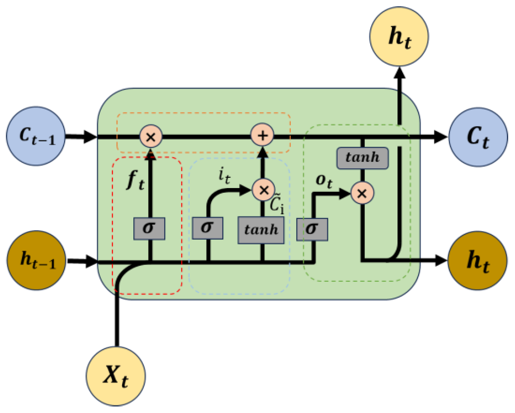
3.1. LSTM Deep Learning Method

LSTM was proposed by Sepp Hochreiter and Jurgen Schmidhuber in 1997 [61]. As a special type of recurrent neural network (RNN), LSTM not only features the external RNN recurrence but also an internal “LSTM cell” recurrence (self-loop). Its unique gating structure (Figure 3) allows it to capture temporal relationships and more easily learn long-term dependencies. The gating structure of LSTM at time t includes the input gate ($i_t$), forget gate ($f_t$), and output gate ($o_t$).

The forget gate ($f_t$) is responsible for controlling the self-loop weight of the state unit ($C_{t-1}$) by setting the weight to a value between 0 and 1 using a sigmoid unit, thus allowing flexible control of state retention and forgetting:

$$f_t=\sigma \left(W_f·\left[h_{t-1},x_t\right]+b_f\right),$$

(1)

where $x_t$ is the current input vector at the t time; $h_{t-1}$ is the output signal of the LSTM at the t − 1 time; and $W_f$ and $b_f$ indicate the weight and bias of the forgetting gate. The role of the input gate ($i_t$) is opposite to that of $f_t$; it determines which information from the new inputs $x_t$ and $h_{t-1}$ should be retained:

$$i_t=\sigma \left(W_i·\left[h_{t-1},x_t\right]+b_i\right),$$

(2)

$${\tilde{C}}_i=tanh\left(W_C·\left[h_{t-1},x_t\right]+b_C\right),$$

(3)

where ${\tilde{C}}_i$ is the candidate cell state; the $W_i$ and $W_C$ are the weight matrixes for the input gate and candidate state, respectively; the $b_i$ and $b_C$ are bias terms for the input gate and candidate state, respectively; the $\sigma$ represents the sigmoid activation function; and the tanh represents the hyperbolic tangent function.

The update mechanism of $i_t$ is similar to that of $f_t$ (obtaining values between 0 and 1 through a sigmoid neural network layer), but it has independent parameters, as shown in Figure 3. The output of $i_t$ is determined by the outputs of the two neural network layers: (1) the $\sigma$ neural network layer (with neural network parameters $W_i$ and $b_i$) and (2) the $tanh$ neural network layer (with neural network parameters $W_C$ and $b_C$). $i_t$ is multiplied by ${\tilde{C}}_i$ to select what information will be added to the cell state $C_t$ at the $t$ time. After completing $f_t$ and $i_t$, the cell status ($C_t$) at the t time will be updated:

$$C_t=f_t\ast C_{t-1}+i_t\ast {\tilde{C}}_i,$$

(4)

$$o_t=\sigma \left(W_O·\left[h_{t-1},x_t\right]+b_O\right),$$

(5)

$$h_t=o_t\ast tanh\left(C_t\right).$$

(6)

where $b_O$ is the bias term for the output gate and $o_t$ is the output gate output. The $f_t$ is multiplied with the $C_{t-1}$, When $f_t$ is 0, it means that the information will be forgotten. After the information selected by $f_t$ is added to the output of $i_t$, a new $C_t$ is obtained (Equation (4)) and $C_t$ will continue to be transmitted to the LSTM network at the $t+1$ moment as a new cell state, i.e., $C_{t+1}$. The output gate $o_t$ is jointly determined by the hidden state $h_{t-1}$ at the previous moment and the current input $x_t$ (Equation (5)). The gating signal $o_t$ is then element-wise multiplied with the cell state $tanh\left(C_t\right)$ processed by the hyperbolic tangent function, obtaining the network output $h_t$ at the current time step (Equation (6)). $h_t$ is also passed to the next stage as the input signal at the next moment.

3.2. SHAP Interpretability Method

In the research on the interpretability of machine learning models, the Shapley Additive Explanations (SHAP) method, as a cooperative game framework based on game theory, provides a theoretically rigorous, intuitive, and effective analytical tool for understanding the prediction mechanism of complex models [62]. The core idea of this method originates from the Shapley value theory. By quantifying the marginal contribution of each feature in a specific prediction scenario, a causal correlation explanation system between the features and the model output is constructed. The weighted average of the marginal contributions of features in all subset combinations is called the SHAP value, and the specific formula is as follows:

$${\varnothing }_i={\sum }_{S\subseteq F\setminus \left\{i\right\}}{\displaystyle \frac{\left|S\right|!\left(\left|F\right|-\left|S\right|-1\right)!}{\left|F\right|!}}\left[f_{S\cup \left\{i\right\}}\left(x_{S\cup \left\{i\right\}}\right)-f_S\left(x_S\right)\right]$$

(7)

where $i$ refers to variables (FVC, PRE, LST, and ET); ${\varnothing }_i$ refers to the SHAP value of the variable $i$; $F$ refers to the set of variables such as FVC, PRE, LST, and ET; $S$ is a subset that does not contain variable $i$ (for example, when calculating the SHAP value of FVC, $S$ can be an empty set, {PRE},{LST},{ET},{PRE, LST},{PRE, ET},{LST, ET}); $x_S$ represents the values of the input features in the set $S$; $F\setminus \left\{i\right\}$ excludes the set of $\left\{i\right\}$; ${\displaystyle \frac{\left|S\right|!\left(\left|F\right|-\left|S\right|-1\right)!}{\left|F\right|!}}$ is a weight term; and $f_{S\cup \left\{i\right\}}\left(x_{S\cup \left\{i\right\}}\right)-f_S\left(x_S\right)$ is the marginal contribution of variable $i$ to subset $S$.

In terms of result presentation, the SHAP method provides a variety of multi-dimensional visualization solutions to support interpretability requirements at different levels. This study adopts a Summary Plot to present the ranking of feature importance in the form of a scatter matrix. The horizontal axis represents the distribution of SHAP values, and the vertical axis represents the feature ranking. The size of the feature values is color-coded, which can simultaneously reveal the global influence and local heterogeneity of the features.

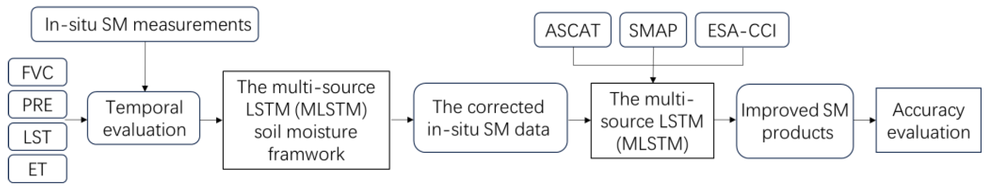
3.3. MLSTM Soil Moisture Calibration Algorithm

To improve the ASCAT, ESA–CCI, and SMAP SM product datasets, this study proposes a MLSTM SM framework by combining satellite remote sensing product data (i.e., the satellite SM, FVC, ET, PRE, and LST) with in-situ SM measurement data. The framework consists of two main steps, (a) and (b), as shown in Figure 4.

Step (a): Considering that the in-situ SM measurements are point-scale data and the satellite product data are pixel-scale data, there exists a scale difference between the two. To obtain the “true” SM values in the grid scale of the ASCAT, ESA–CCI, and SMAP SM products, this study first used the average value of the in-situ SM measurement data within the same grid of the satellite SM product as this grid’s SM. Then, this study used the PRE, LST, FVC, ET, and the grid’s SM data as inputs of LSTM to train the LSTM for the correction of the point-scale in-situ SM dataset in SMAP 0.1°, ASCAT 0.1°, and ESA–CCI 0.25° grid scales, respectively. At the same time, the in-situ SM loss data in the SMAP 0.1°, ASCAT 0.1°, and ESA–CCI 0.25° grid scales after training, compared with the original in-situ SM measurements in point scale, were also obtained.

When executing the LSTM deep learning method, the setting of its hyperparameters was involved. During manual tuning, parameters were iteratively optimized by systematically observing training dynamics and model performance. The hyperparameters of the LSTM models used in this study were listed based on ASCAT grid data for full-variable station-scale SM estimation (

Table 2. The setting strategy of the LSTM’s hyperparameters.

	Hyperparameters	CTP–SMTMN	HOBE	OZNET	SNOTEL
1	Learning Rate	0.001	0.001	0.01	0.001
2	Hidden Size	100	100	100	100
3	Batch Size	1	4	2	3
4	Epochs	100	100	110	130
5	Sequence Length	180	90	180	50
6	Dropout	0.2	/	0.2	0.2
7	optimizer	Adam	Adam	Adam	Adam
8	activation	sigmoid	ReLU	sigmoid	sigmoid

).

The adjustment strategy for the LSTM’s hyperparameters in this study was as follows: (1) the learning rate was typically adjusted based on the convergence speed and stability of the training loss. Specifically, when the loss exhibited significant fluctuations or failed to decrease consistently, the learning rate was reduced. Conversely, if convergence was excessively slow, the learning rate was increased. In this study, a learning rate of 0.001 was adopted for the CTP–SMTMN, HOBE, and SNOTEL datasets, while a relatively larger value of 0.01 was used for OZNET to accelerate training. (2) The hidden size was selected by balancing model complexity and task difficulty. A consistent hidden size of 100 units was used across all datasets (CTP–SMTMN, HOBE, OZNET, and SNOTEL) to ensure sufficient representational capacity. When validation performance was suboptimal, the number of neurons could be increased incrementally, with the validation loss closely monitored to avoid overfitting. (3) Batch size was tuned to achieve an appropriate trade-off between training efficiency and gradient stability. Larger batch sizes typically accelerate the training process, but they might reduce the model’s generalization ability. A small batch size of 1 was used for CTP–SMTMN, while batch sizes of 4, 2, and 3 were employed for HOBE, OZNET, and SNOTEL, respectively, based on dataset size and memory constraints. Smaller batch sizes may improve generalization, but often require more careful tuning of the learning rate. (4) The number of training epochs was determined using early stopping criteria. Specifically, 100 epochs were used for CTP–SMTMN and HOBE, 110 for OZNET, and 130 for SNOTEL, allowing for sufficient model convergence while preventing overfitting. (5) Sequence length was optimized according to the characteristics of the input data and the limitation of computational resources. A sequence length of 180 was applied for CTP–SMTMN and OZNET, whereas shorter lengths of 90 and 50 were used for HOBE and SNOTEL, respectively, to reduce memory usage and mitigate redundancy. (6) The dropout rate was adjusted based on the model’s capacity. A higher dropout rate (e.g., 0.3–0.5) was employed to prevent overfitting, while a lower rate was adopted in scenarios indicating underfitting. A dropout of 0.2 was applied to CTP–SMTMN, OZNET, and SNOTEL, but omitted for HOBE, possibly due to a smaller model or reduced risk of overfitting in that context. (7) Optimizer selection was task-dependent, with Adam employed as the default. (8) The choice of activation function had a direct impact on the model’s ability to learn nonlinear connections. For example, in situations where vanishing gradients arose from saturated outputs from sigmoid or tanh functions, ReLU activation was adopted as a more effective alternative. Therefore, the sigmoid was employed for CTP–SMTMN, OZNET, and SNOTEL while ReLU was used for HOBE because of the vanishing gradient issues. Throughout the training process, both model accuracy and convergence behavior were monitored to achieve an optimal synergy among hyperparameters. The overarching goal was to attain the best possible generalization performance within the constraints of available computational resources.

Step (b): Three SM product datasets (i.e., ASCAT, SMAP, and ESA–CCI) were used as input for the LSTM with the same hyperparameters (i.e., Table 2) used to train the LSTM and obtain the loss data of the ASCAT, SMAP, and ESA–CCI SM products, respectively. Then, the loss data of ASCAT, SMAP and ESA–CCI SM products were compared and adjusted with the SM loss data obtained in Step (a) using the MSE (Equation (8)):

$$L={\displaystyle \frac{1}{N}}{\sum }_{i=1}^N{\left(y_i-\widehat{y_i}\right)}^2$$

(8)

where $N$ is the total number of samples; $y_i$ represents the SM loss data obtained in Step (a) of $i$ samples; and $\widehat{y_i}$ represents the loss data of the ASCAT (or SMAP or ESA–CCI) SM product of $i$ samples. When the MSE value reached its minimum, we considered the improved ASCAT, SMAP, and ESA–CCI SM products to be the optimal SM products.

Additionally, to explore the impacts of key auxiliary variables i.e., FVC, PRE, LST, and ET on the improved ASCAT, SMAP and ESA–CCI obtained in Step (b), these four key auxiliary variables were combined and divided into five cases: (1) FVC, PRE, LST, and ET (called FPLE); (2) LST, ET, and FVC (called LEF); (3) LST, ET, and PRE (called LEP); (4) LST, PRE, and FVC (called LPF); (5) PRE, ET, and FVC (called PEF). The three or four variables were used as the inputs to LSTM in Step (a) to train the LSTM model and obtain the SM loss data under five cases, which were then compared with the loss data of the ASCAT (or SMAP or ESA–CCI) SM product obtained in Step (b). We also considered the construction of MLSTM models under single variable and bivariate combinations, but found that the results were not ideal. Therefore, we chose three-variable and four-variable combinations. In addition, in order to quantitatively analyze the impact of different variables on the MLSTM model, the combinations of three and four variables make it easier to compare which of the four variables, PRE, ET, FVC, and LST, is the dominant factor affecting the MLSTM model.

3.4. Evaluation Metrics

The six metrics, i.e., MAE (Mean Absolute Error, cm³/cm³), RMSE (cm³/cm³), ubRMSE (unbiased Root Mean Square Error, cm³/cm³), Bias (cm³/cm³), SD (cm³/cm³), and R were used to evaluate the corrected in-situ SM data in the ASCAT 0.1°, SMAP 0.1°, and ESA–CCI 0.25° grid scales and the final improved ASCAT, SMAP, and ESA–CCI SM product datasets (Equations (9)–(14)):

$$MAE={\displaystyle \frac{1}{n}}{\sum }_{i=1}^n\left|y_i-\widehat{y_i}\right|$$

(9)

$$RMSE=\sqrt{{\displaystyle \frac{1}{n}}{\sum }_{i=1}^n{(y_i-\widehat{y_i})}^2 }$$

(10)

$$ubRMSE=\sqrt{{\displaystyle \frac{1}{n-1}}{\sum }_{i=1}^n{(y_i-\widehat{y_i})}^2 }$$

(11)

$$Bias={\displaystyle \frac{1}{n}}{\sum }_{i=1}^n\left(y_i-\widehat{y_i}\right)$$

(12)

$$SD=ubRMSE=\sqrt{{\displaystyle \frac{1}{n-1}}{\sum }_{i=1}^n{(y_i-\overline{y})}^2 }$$

(13)

$$R={\displaystyle \frac{{\sum }_{n-1}^n\left(y_i-\overline{y}\right)\left(\widehat{y_i}-\overline{\widehat{y}}\right)}{\sqrt{{\sum }_{i=1}^n{\left(y_i-\overline{y}\right)}^2}\sqrt{{\sum }_{i-1}^n{\left(\widehat{y_i}-\overline{\widehat{y}}\right)}^2}}}$$

(14)

where $y_{obs,i}$ is the in-situ SM value at the i-th point; $y_{pred,i}$ is the predicted SM value at the i-th point; $n$ is the total number of samples; $y_i$ is the in-situ SM value (raw and predicted satellite data) at the i-th point; $\overline{y}$ is the mean of in-situ SM value (raw and predicted satellite data); $\overline{y_{obs}}$ is the mean of the in-situ SM values; and $\overline{y_{pred}}$ is the mean of the predicted SM values.

4. Results

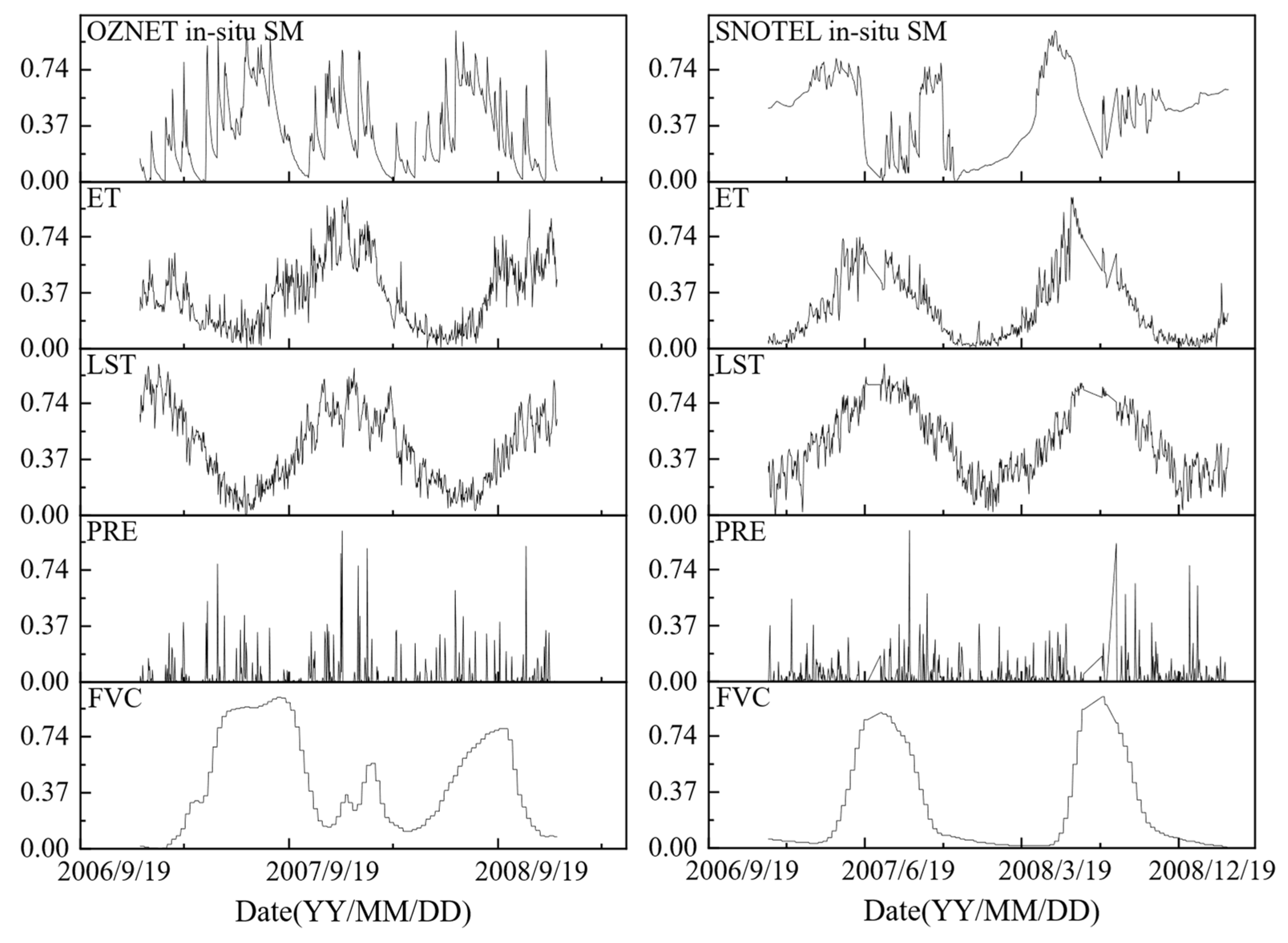
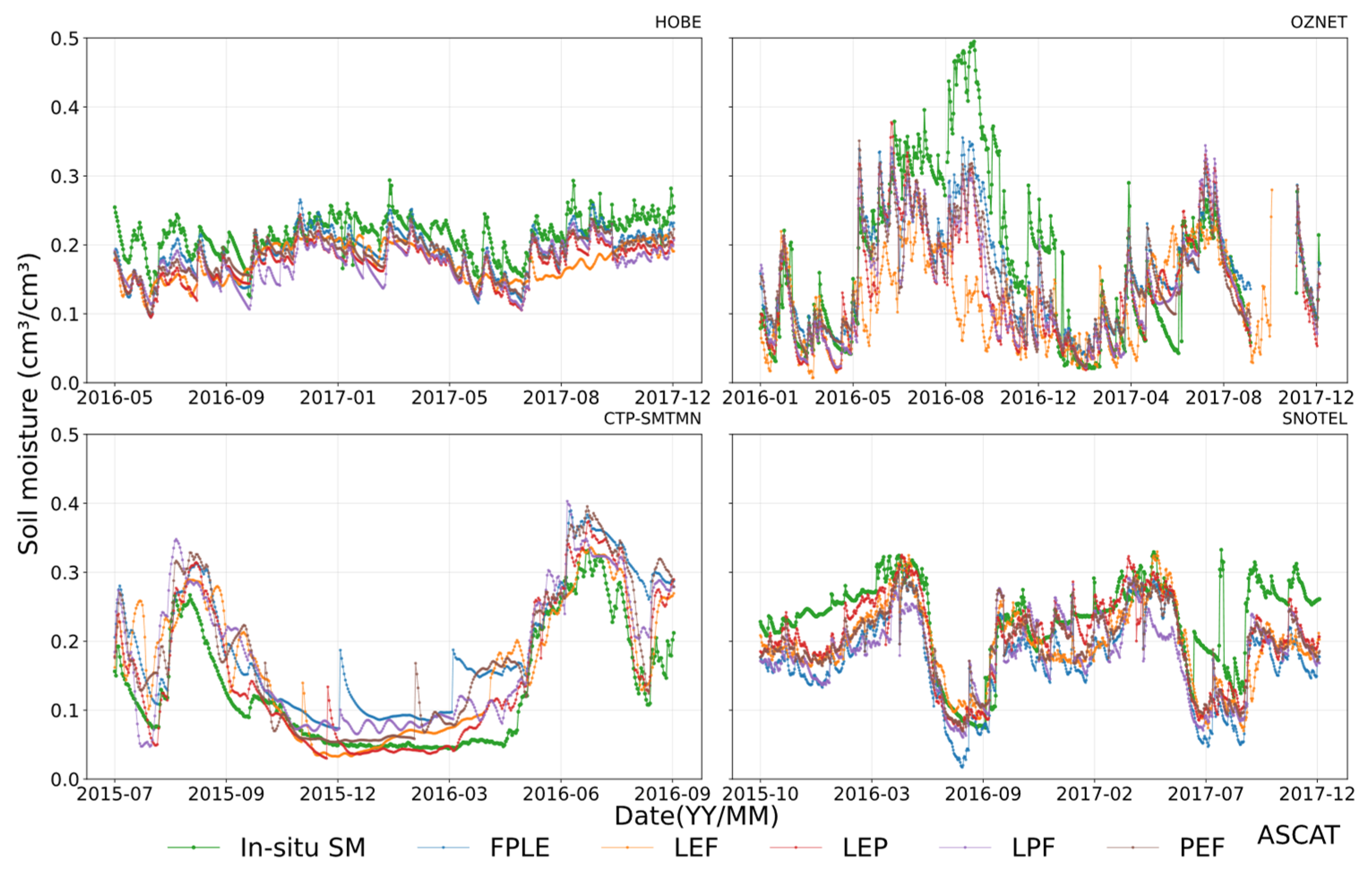
4.1. Temporal Evolutions of FVC, PRE, LST, ET, and In-Situ SM Measurements

Due to the inconsistent units of the in-situ SM measurements FVC, LST, ET, and PRE, for comparing their temporal evolution characteristics, the temporal evolutions of the normalized in-situ SM measurements FVC, LST, ET, and PRE are shown in Figure 5. The normalization calculation formula is $X^{\prime }=(X-X_{min})/(X_{max}-X_{min})$, where $X^{\prime }$, $X$, $X_{min}$ and $X_{max}$ are the normalized value, original value, the minimum and maximum of in-situ SM measurements (FVC, LST, ET, or PRE), respectively.

The change rule of in-situ SM measurement data was almost synchronous with the PRE of the CTP–SMTMN, HOBE, OZNET, and SNOTEL observation networks. Whenever there was an increase or decrease in PRE, the in-situ SM measurement data also increased or decreased, indicating that PRE was a primary driving factor directly influencing SM variability, a key force in the data directly affecting the SM. In contrast, the FVC and ET exhibited more gradual temporal changes and tended to impact SM and LST with a noticeable time lag. This delayed response to SM likely reflects the physical process underlying vegetation growth and water transfer, which require time to manifest after changes in SM availability and surface energy balance. Despite this lag, the seasonal trends of FVC and ET still remained consistent with SM. For example, during winter (November to March of the next year), the normalized SM values of the CTP–SMTMN network dropped below 0.1, accompanied by normalized FVC and ET values below 0.05 and 0.1. In summer (June to September), the normalized SM exceeded 0.8, and both the normalized FVC and ET values rose accordingly, reaching values above 0.8 and 0.6. These patterns emphasize the strong coupling between PRE, FVC, ET, LST, and SM, although their temporal responses vary due to differing physical mechanisms.

In addition, this study conducted a correlation analysis by calculating the R value (Equation (14)) between FVC, ET, LST, PRE, and the in-situ SM measurements at the CTP–SMTMN, HOBE, OZNET, and SNOTEL observation networks (

Table 3. Correlation coefficients between the precipitation (PRE), surface temperature (LST), vegetation coverage (FVC), evapotranspiration (ET), and in-situ SM measurements at the CTP–SMTMN, HOBE, OZNET, and SNOTEL observation networks.

Variables\Networks	CTP–SMTMN	OZNET	HOBE	SNOTEL
FVC	0.720 **	0.501 **	0.089 *	−0.162 **
PRE	0.419 **	0.217 **	0.195 **	0.086 *
LST	0.559 **	−0.536 **	0.214 **	0.090 *
ET	0.746 **	−0.060	0.030	0.367 **

** At the level of 0.01 (double-tailed), the correlation is significant. * At the level of 0.05 (two-tailed), the correlation is significant.

).

4.2. Correction of In-Situ Soil Moisture Measurements

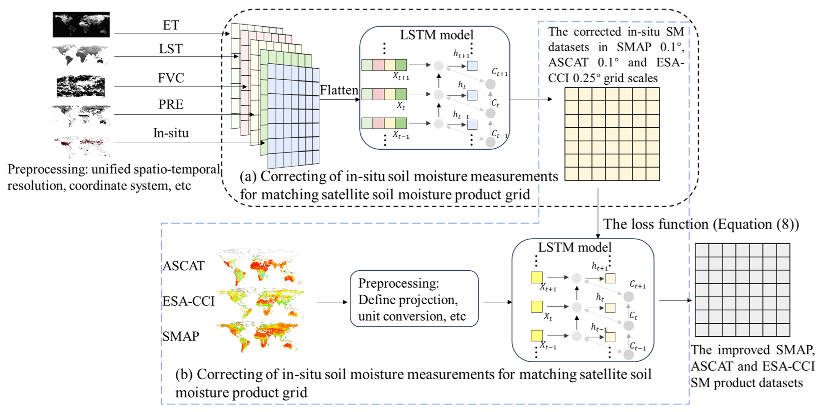
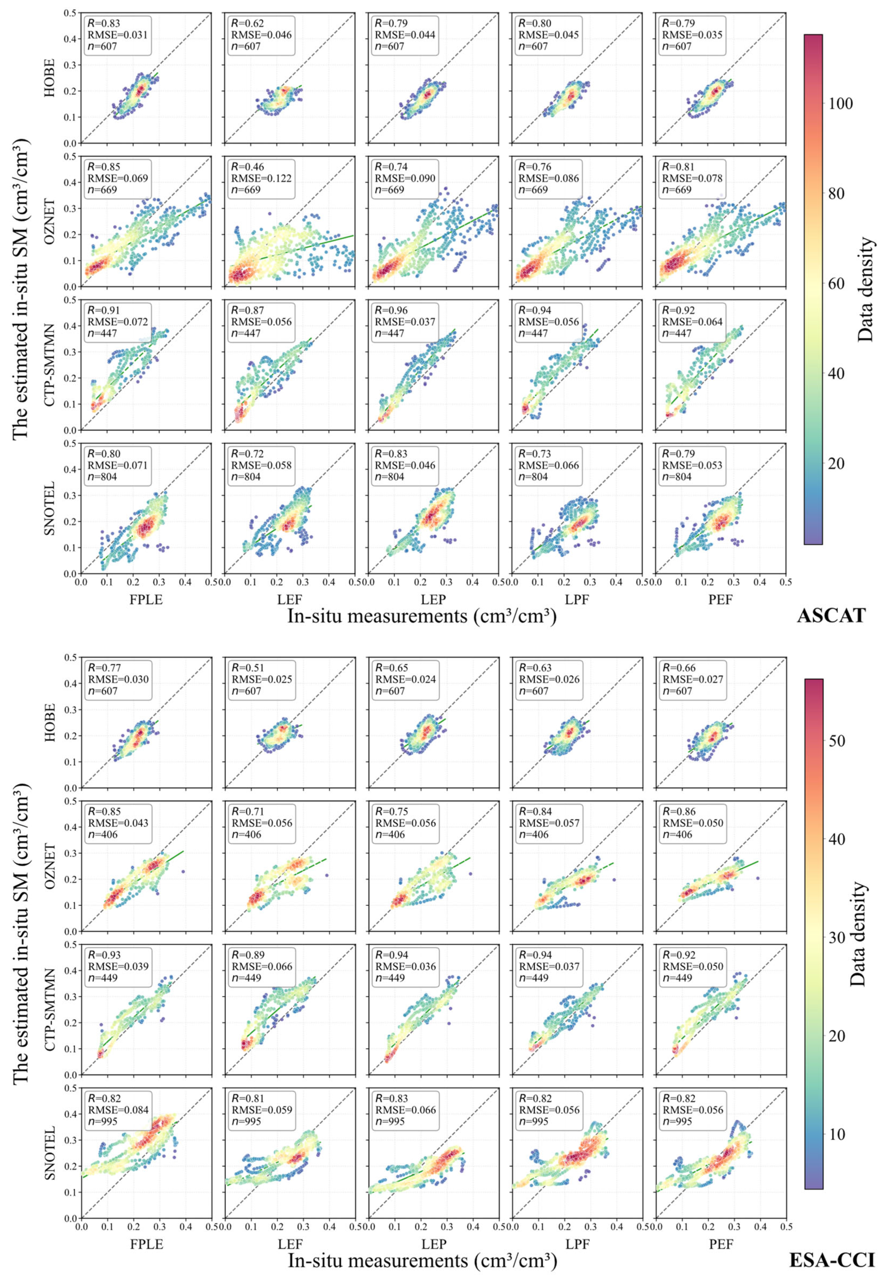
4.2.1. Correction of In-Situ SM Measurements for Matching Satellite SM Product Grid

To obtain the “true” SM values matching the grid sizes of the ASCAT (0.1°), ESA–CCI (0.25°), and SMAP (0.1°) SM products, this study corrected in-situ SM measurements and obtained the loss SM data using the LSTM model. In addition, the corrected in-situ SM data under five variable combinations, i.e., FPLE (FVC, PRE, LST, and ET), LEF (LST, ET, and FVC), LEP (LST, ET, and PRE), LPF (LST, PRE, and FVC), and PEF (PRE, ET, and FVC), were compared with original in-situ SM measurements using five evaluation metrics, i.e., R, MAE, RMSE, ubRMSE, and Bias (Equations (9)–(14)). The calculated metric values were shown in

Table 4. The calculated R, MAE (cm³/cm³), RMSE (cm³/cm³), ubRMSE (cm³/cm³), and Bias (cm³/cm³) values between the estimated in-situ SM data matching satellite SM product grids (i.e., ASCAT 0.1°, SMAP 0.1°, ESA–CCI 0.25°) against original in-situ SM measurements at the HOBE, OZNET, CTP–SMTMN, and SNOTEL observation network.

Network	Variable Combination	ASCAT 0.1°Grid					ESA–CCI 0.25°Grid					SMAP 0.1° Grid
		R	MAE	RMSE	ubRMSE	Bias	R	MAE	RMSE	ubRMSE	Bias	R	MAE	RMSE	ubRMSE	Bias
HOBE	FPLE	0.831	0.027	0.031	0.018	0.025	0.767	0.025	0.030	0.019	0.023	/	/	/	/	/
	LEF	0.618	0.040	0.046	0.024	0.039	0.515	0.020	0.025	0.025	0.003	/	/	/	/	/
	LEP	0.794	0.041	0.044	0.016	0.041	0.650	0.019	0.024	0.024	0.001	/	/	/	/	/
	LPF	0.795	0.041	0.045	0.019	0.041	0.630	0.021	0.026	0.025	0.008	/	/	/	/	/
	PEF	0.787	0.031	0.035	0.020	0.029	0.656	0.022	0.027	0.022	0.015	/	/	/	/	/
OZNET	FPLE	0.845	0.053	0.069	0.067	0.017	0.854	0.053	0.043	0.037	0.052	0.821	0.055	0.070	0.040	−0.051
	LEF	0.464	0.084	0.122	0.106	0.061	0.711	0.043	0.056	0.052	0.021	0.725	0.035	0.044	0.043	−0.010
	LEP	0.745	0.059	0.090	0.078	0.036	0.754	0.040	0.056	0.048	0.028	0.767	0.032	0.039	0.036	−0.016
	LPF	0.764	0.059	0.086	0.077	0.038	0.842	0.045	0.057	0.043	0.037	0.843	0.033	0.040	0.032	−0.024
	PEF	0.807	0.057	0.078	0.073	0.027	0.865	0.042	0.050	0.045	0.021	0.814	0.027	0.032	0.031	−0.009
CTP–SMTMN	FPLE	0.909	0.061	0.072	0.038	−0.061	0.931	0.030	0.039	0.031	−0.023	/	/	/	/	/
	LEF	0.872	0.041	0.056	0.046	−0.032	0.889	0.056	0.066	0.030	−0.053	/	/	/	/	/
	LEP	0.964	0.028	0.037	0.030	−0.021	0.941	0.027	0.036	0.031	−0.019	/	/	/	/	/
	LPF	0.939	0.047	0.056	0.033	−0.045	0.942	0.031	0.037	0.028	−0.024	/	/	/	/	/
	PEF	0.916	0.050	0.064	0.042	−0.048	0.920	0.040	0.050	0.035	−0.036	/	/	/	/	/
SNOTEL	FPLE	0.800	0.061	0.071	0.039	0.059	0.824	0.071	0.084	0.054	−0.064	0.866	0.026	0.033	0.031	−0.010
	LEF	0.724	0.047	0.058	0.045	0.037	0.809	0.047	0.059	0.059	−0.006	0.850	0.032	0.041	0.032	−0.026
	LEP	0.825	0.035	0.046	0.037	0.027	0.835	0.058	0.066	0.058	0.031	0.867	0.027	0.031	0.030	0.006
	LPF	0.728	0.059	0.066	0.042	0.051	0.820	0.044	0.056	0.055	−0.010	0.876	0.030	0.039	0.030	−0.025
	PEF	0.786	0.044	0.053	0.039	0.036	0.819	0.044	0.056	0.056	0.002	0.777	0.033	0.044	0.038	−0.022

FPLE is the combination of FVC, PRE, LST, and ET; LEF is the combination of LST, ET, and FVC; LEP is the combination of LST, ET, and PRE; LPF is the combination of LST, PRE, and FVC, and PEF is the combination of PRE, ET, and FVC.

. The number of in-situ sites used for LSTM training and validation are as follows: CTP–SMTMN (19 training and 31 validation), HOBE (9 training and 20 validation), OZNET (5 training and 10 validation), and SNOTEL (6 training and 23 validation).

At the CTP–SMTMN network, the LEP combination yielded the best performance across both the ASCAT (0.1°) and ESA–CCI (0.25°) grids, with the highest R values (0.946 and 0.941), and the lowest MAE, RMSE, ubRMSE, and Bias values compared to the FPLE, LEF, LPF, and PEF combinations. This suggests that the FVC contributed little to SM estimation at this site, possibly due to either its low relevance or poor data quality, which may have introduced noise into the LSTM. Similarly, for the SMAP (0.1°) grid, the PEF combination showed superior performance in the OZNET and SNOTEL networks, with significantly lower error metrics (e.g., MAE = 0.027 cm³/cm³, RMSE = 0.032 cm³/cm³, ubRMSE = 0.045 cm³/cm^3,, and Bias = −0.009 cm³/cm³) compared to the FPLE combination (MAE = 0.055 cm³/cm³, RMSE = 0.070 cm³/cm³, ubRMSE = 0.119 cm³/cm³, and Bias = −0.051 cm³/cm³). However, in the HOBE and OZNET networks, the FPLE combination achieved the best results under the ASCAT (0.1°) and ESA–CCI (0.25°) grids, with R values of 0.831 and 0.845, respectively, indicating the FVC, ET, LST, and PRE as inputs of LSTM contributed meaningfully to LSTM.

Overall, LSTM performance varied significantly with different variable combinations and grids of ASCAT (0.1°), ESA–CCI (0.25°), and SMAP (0.1°) products. Notably, ESA–CCI (0.25°) and SMAP (0.1°) consistently outperformed ASCAT (0.1°) in terms of lower MAE and RMSE values. For instance, under the LEF combination in the HOBE, the MAE from ESA–CCI (0.020 cm³/cm³) was significantly lower than ASCAT (0.040 cm³/cm³), suggesting closer alignment with the in-situ SM measurements.

In addition, the scatter and temporal evolution plots (Figure 6 and Figure 7) were drawn to further show the differences between the estimated in-situ SM data using LSTM and original in-situ SM measurements under the FPLE, LEF, LPF, and PEF combinations in the ASCAT (0.1°), SMAP (0.1°), and ESA–CCI (0.25°) grids in the HOBE, OZNET, CTP–SMTMN, and SNOTEL observation networks.

At the ASCAT (0.1°) grid, under the FPLE combination, the estimated in-situ SM was more consistent with the original in-situ SM measurements. However, in the LEF combination (excluding PRE), the estimated in-situ SM showed poorer consistency with the original in-situ SM measurements, particularly in the OZNET network, where a significant disadvantage is evident (R = 0.464 and RMSE = 0.122 cm³/cm³). This underscores the importance of PRE for SM estimation. The temporal evolutions indicate consistent deviations during the crop irrigation period (July to September). Under the SMAP (0.1°) grid, in the OZNET network under the LEF combination, the temporal evolution curve is the flattest. In the SNOTEL network, most of the temporal evolution curves are overestimated, especially in the low SM values around August 2020, with the LEF combination being the most severely overestimated. Comparative analysis using ESA–CCI (0.25°) revealed that reduced spatial resolution and increased regional heterogeneity impaired model accuracy in HOBE, where the average R-values across variable combination to 0.644–0.765. Conversely, OZNET showed the improvement under ESA–CCI, with the average R-values increasing to 0.725–0.808, potentially due to reduced SM variability at coarser scales.

4.2.2. Contribution Analysis of Auxiliary Variables to MLSTM Using the SHAP Method

We applied the SHAP to interpret the MLSTM predictions by calculating the marginal contribution of each variable (PRE, FVC, ET, or LST). SHAP values were calculated and visualized for all SM estimates in the ASCAT (Figure 8). The plot ranks variable importance from top to bottom, the color indicating the original variable value, and the X axis showing the SHAP value, i.e., its influence on the prediction.

In the HOBE network, the LST consistently shows the highest contribution across most combinations. For example, under the FPLE and LEF combinations (Figure 8(a1,a2)), LST not only ranks highest in importance but also shows a strong gradient in SHAP value distribution, indicating a stable and interpretable influence. In the OZNET network, FVC has the greatest influence (Figure 8(b1–b5)) and PRE has the least influence. In the CTP network, the influence of FVC and ET is close and the influence of PRE is the smallest (Figure 8(c1–c5)). ET has a great influence on the SNOTEL network (Figure 8(d1,d4)).

SHAP values are widely scattered, and high-value (red) and low-value (blue) points appear intermixed along the X-axis under the LEF combination. For instance, in HOBE (Figure 8(a2)) and OZNET (Figure 8(b2)), this chaotic distribution suggests that regardless of the original values of LST, ET, or FVC, their influence on SM estimation is unpredictable—highlighting poor model interpretability. This aligns with the poor performance of the LEF combination reported earlier (e.g., R = 0.464 for OZNET in Figure 6). Overall, although PRE often appears less important in SHAP rankings, models that exclude it tend to yield inferior results. The PRE is one of the most direct influencing factors of SM; it can effectively fit the overall trend. The LST, ET, and FVC factors can optimize the details. Omitting PRE leads to unstable contributions and weaker generalization, especially in networks with pronounced climatic variability or anthropogenic impacts (e.g., irrigation in OZNET).

4.3. The Improved ASCAT, SMAP, and ESA–CCI Products

4.3.1. Violin Plots of the Improved ASCAT, SMAP, and ESA–CCI Products

Based on the corrected in-situ SM datasets in Section 4.2, which could match the ASCAT (0.1°), SMAP (0.1°), and ESA–CCI (0.25°) grids, the ASCAT, ESA–CCI, and SMAP SM products were improved using the loss SM data obtained from in-situ SM measurements (Figure 6 and Figure 7 and Equation (4)). The RMSE and R violin plots of the improved ASCAT, ESA–CCI, and SMAP SM products against the corrected in-situ SM data were shown in Figure 9.

In the SNOTEL network, the ASCAT LEP combination had the best performance, with a mean R value close to 0.8 with a mean RMSE near 0.030 cm³/cm³, accompanied by a tight distribution, indicating both accuracy and stability. Conversely, the LEF combination showed the poorest performance, with the largest R-value dispersion (interquartile range reaching 0.5) and higher RMSE variability (approximately 0.025 cm³/cm³), indicating notable instability. For SMAP and ESA–CCI, the LEP combination also yielded solid results, with a mean R-value around 0.7 and mean RMSE values of 0.060 and 0.045 cm³/cm³, respectively. In the OZNET network representing Australian plains environments, the ASCAT’s LEF combination again underperformed, with a mean R value of approximately 0.7 and RMSE around 0.045 cm³/cm³, while SMAP’s FPLE combination showed an elevated RMSE (0.045 cm³/cm³), suggesting that excessive auxiliary variables may introduce redundant information or noise. In contrast, the LEF combination showed superior performance, with an R-value exceeding 0.8 and RMSE around 0.030 cm³/cm³. In the CTP–SMTMN network, ESA–CCI performed best, with a mean R value around 0.85 and RMSE below 0.030 cm³/cm³, followed by ASCAT with a mean R value around 0.80. In the HOBE network, the results mirrored OZNET: ASCAT’s LEF combination performed poorly (mean R ~ 0.5), while ESA–CCI maintained stable performance (mean R ~ 0.8 and RMSE ~ 0.02 cm³/cm³).

Overall, the LEP combination consistently outperformed the others, while LEF combinations lacking PRE led to unstable and less accurate estimates, reinforcing the pivotal role of PRE. Additionally, SNOTEL exhibited larger uncertainties due to geographic heterogeneity, emphasizing the importance of accuracy in in-situ SM data that can match the grids of satellite SM products.

4.3.2. Spatial Distributions of the Improved ASCAT, SMAP, and ESA–CCI Products

The spatial comparison of the original and improved ASCAT, ESA–CCI, and SMAP SM products on 9 September 2016, across CTP–SMTMN (China), OZNET (Australia), HOBE (Denmark), and SNOTEL (USA) networks is shown in Figure 10.

The improved ASCAT, ESA–CCI, and SMAP SM products can capture more detailed SM and better reflect spatial variations of SM. For example, in the CTP–SMTMN and OZNET regions, the improved ASCAT and SMAP products exhibit a clearer gradient and better continuity. In the SNOTEL region, the improved ASCAT, ESA–CCI, and SMAP SM products retain more realistic spatial heterogeneity (Figure 10). These results suggest that the MLSTM-based algorithm effectively refines satellite ASCAT, ESA–CCI, and SMAP SM products, particularly in heterogeneous areas.

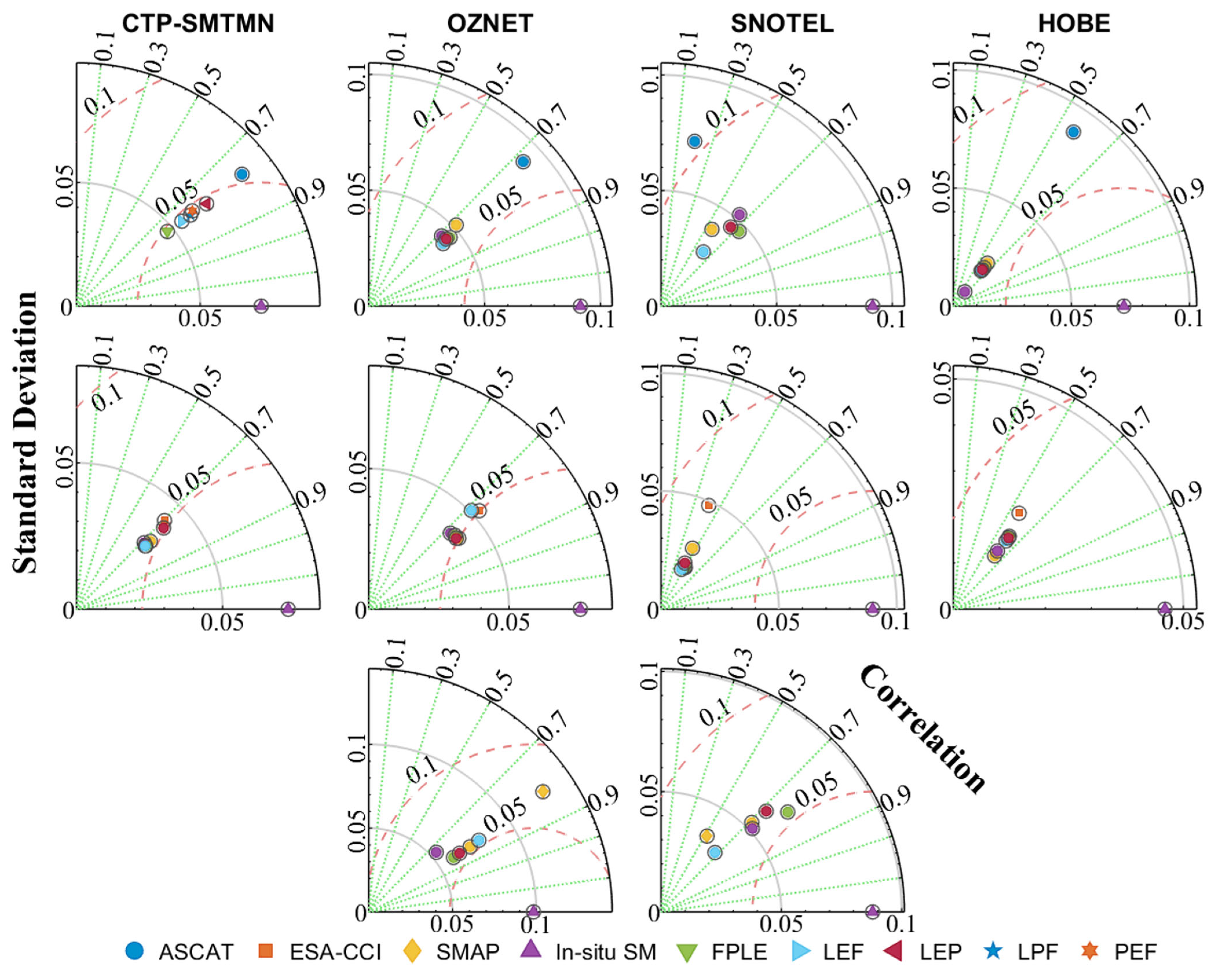
4.4. Evaluation of the Improved ASCAT, ESA–CCI, and SMAP Products

To quantitatively evaluate the improved ASCAT, ESA–CCI, and SMAP SM products, this study employed the Taylor Diagram, which comprehensively displays the differences of improved and original ASCAT, ESA–CCI, and SMAP products with in-situ SM measurements (i.e., reference data) through a combination of SD, R, and RMSD (Figure 11).

The optimal variable combinations for an MLSTM framework vary across satellite SM products and in-situ observation networks. For example, the best variable combinations are LEP in ASCAT’s OZNET and SNOTEL, FPLE in HOBE, and LPF in CTP–SMTMN. In ESA–CCI, FPLE performs best in OZNET and SNOTEL, while LEP, and PEF are optimal in HOBE and CTP–SMTMN, respectively. For SMAP, LPF and LEP yield the best results in OZNET and SNOTEL, respectively. Although the R values among improved ASCAT, ESA–CCI, and SMAP SM products are similar (e.g., 0.77 in ASCAT’s CTP-STMN), the SD and RMSD vary significantly. For example, in CTP–SMTMN and HOBE networks, under the LEP combination, the improved ASCAT SM values align better with in-situ measurements in terms of SD. Similar improvements are seen in ESA–CCI’s HOBE and SNOTEL and SMAP’s OZNET networks. Overall, the improved ASCAT and SMAP SM products were more consistent with in-situ SM measurements, while the ESA–CCI product shows limited room for improvement due to the influence of surface heterogeneity.

In addition, this study calculated the RMSD of the improved ASCAT, ESA–CCI, and SMAP SM products against in-situ SM measurements (

Table 5. The calculated RMSD (Root Mean-Square Deviation, cm³/cm³) values between improved ASCAT, ESA–CCI, SMAP SM data, and in-situ SM measurements of CTP–SMTMN, HOBE, OZNET, and SNOTEL networks under five variable combinations i.e., FPLE (FVC, PRE, LST, and ET), LEF (LST, ET, and FVC), LEP (LST, ET, and PER), LPF (LST, PRE, and FVC), PEF (PRE, ET, and FVC).

Satellite	Network	Original	FPLE	LEF	LEP	LPF	PEF
ASCAT	HOBE	0.0768	0.0606	0.0677	0.0614	0.0623	0.0619
	OZNET	0.0670	0.0640	0.0671	0.0635	0.0651	0.0647
	CTP–SMTMN	0.0539	0.0485	0.0470	0.0469	0.0466	0.0475
	SNOTEL	0.1049	0.0770	0.0698	0.0662	0.0769	0.0702
ESA–CCI	HOBE	0.0379	0.0388	0.0385	0.0373	0.0376	0.0373
	OZNET	0.0502	0.0501	0.0537	0.0518	0.0523	0.0509
	CTP–SMTMN	0.0520	0.0526	0.0543	0.0533	0.0535	0.0509
	SNOTEL	0.0822	0.0806	0.0817	0.0814	0.0828	0.0820
SMAP	OZNET	0.0720	0.0543	0.0681	0.0578	0.0537	0.0563
	SNOTEL	0.0757	0.0625	0.0608	0.0545	0.0700	0.0609

). The following is a detailed description of the calculation formula of RMSD in Taylor’s chart and its related indicators:

$$RMSD=\sqrt{{\sigma }_{model}^2+{\sigma }_{obs}^2-2{\sigma }_{model}{\sigma }_{obs}R}$$

(15)

where ${\sigma }_{model}$ is the SD of the predicted SM value of MLSTM; ${\sigma }_{obs}$ is the SD of in-situ SM measurements; and $R$ is the correlation coefficient between the predicted SM values of MLSTM and the in-situ SM measurements. A lower RMSD indicates a closer match between the predicted SM values of MLSTM and in-situ SM measurements and is consistent with improved model performance in Taylor diagrams.

For the improved ASCAT, all variable combinations yielded substantial improvements over the original ASCAT SM product, with the LEP combinations in the SNOTEL network showing the most notable reduction of RMSD values from 0.1049 to 0.0662 cm³/cm³, corresponding to a 36.89% improvement. Similarly, the SMAP showed significant gains, especially in the OZNET network, where the FPLE and LPF combinations reduced RMSD by more than 20%, and in the SNOTEL network, where the LEP achieved a 28.01% improvement (RMSD values from 0.0757 to 0.0545 cm³/cm³). In contrast, original ESA–CCI, which already had relatively low RMSD values, exhibited more modest improvements. For example, FPLE in the SNOTEL network reduced RMSD by 1.95% and PEF in the CTP–SMTMN network achieved a 2.12% decrease. These results indicate the potential for improvement is limited when the accuracy of original satellite SM product is already high. Overall, the ASCAT and SMAP products benefit more significantly from MLSTM correction, particularly under LEP, FPLE, and LEF combinations, whereas ESA–CCI shows only marginal gains.

5. Discussion

The impact of spatial grid resolution and variable combinations on in-situ SM correction performance varied across satellite SM products and networks. Results for the corrected in-situ SM datasets matched to the grids of ASCAT (0.1°), ESA–CCI (0.25°), and SMAP (0.1°) SM products showed that in the HOBE network, the ASCAT (0.1°) product grid yielded slightly better correction accuracy than ESA–CCI (0.25°). This may be attributed to increased surface heterogeneity at coarse grid resolution (0.25°), which reduces the representativeness of point-scale in-situ SM measurements [63]. For the SMAP grid (0.1°), the performance across variable combinations was more balanced compared to the ASCAT grid (0.1°), potentially due to differences between satellite transit time and in-situ measurement synchronization [64]. Among the tested variable combinations, the LEF combination consistently performed the worst. For example, in ASCAT-based estimations, the R value under LEF in the OZNET network dropped to 0.464, far below other combinations. This confirms precipitation’s critical role in SM modeling [65]. Notably, in the CTP network, the MLSTM SM framework performed well and stably, followed by the SNOTEL network. The in-situ SM values corrected by MLSTM in the CTP–SMTMN network region are often overestimated. One of the reasons for this may be the special climate conditions of cold arid and semi-arid [48] terrain. For instance, under the ASCAT grid (0.1°), the Bias values for FPLE and PEF reached −0.061 and −0.048 cm³/cm³, respectively, compared to −0.021 and −0.045 cm³/cm³ under the LEP and LPF combinations. LST plays a significant role in this cold environment, suggesting that the surface temperature in the cold region controls the freezing and thawing of permafrost [66].

Specific landscape and climate characteristics influenced MLSTM uncertainty and estimation accuracy. The OZNET and HOBE networks performed poorly and were unstable, with the maximum difference in R values between different variable combinations within the same satellite grid reaching 0.381 (OZNET) and 0.252 (HOBE). The speculated reason was as follows: OZNET was located in a rain-fed farmland area, and due to human water resource management, SM fluctuates violently (for example, abnormally high observed values from July to December 2016) [50]. Due to the MLSTM not incorporating irrigation parameters, the improved ASCAT, ESA–CCI, and SM products were often underestimated and did not capture sudden peaks, indicating insufficient characterization of human intervention in existing data [67]. HOBE was located in Denmark and had a temperate maritime climate with stable humidity levels (approximately 0.2 cm³/cm³ throughout the year). However, due to the high heterogeneity of land cover types such as farmland, coniferous forests, grasslands, and forests, the representativeness of the sites may be poor, leading to unstable estimation results [63]. Overall, the results of SM estimation at the site can be used as benchmark data for subsequent experiments. However, although four in-situ observation regions were selected as study areas to construct the MLSTM and analyze the influence of PRE, ET, LST, and FVC for SM estimation, it cannot be guaranteed that the MLSTM can achieve the optimization correction results of ASCAT, SMAP, and ESA–CCI SM products. In the follow-up, more application evaluations of MLSTM need to be conducted according to land cover type and climate zone.

Different variables have specific effects on the improved ASCAT, ESA–CCI, and SMAP SM products, but their respective contributions to the MLSTM were not clear. In the HOBE network, the dominant role of LST was most prominent. The OZNET farmland area was driven by FVC as the core driving factor, with PRE having the lowest marginal contribution. In CTP–SMTMN networks, FVC and ET had similar effects, while PRE had the weakest impact. In the SNOTEL network, the crucial role of ET was highlighted, which may be related to the high forest coverage in the region. Although PRE had a low SHAP value in most scenarios, as a direct moisture input source, it had irreplaceability in trend fitting, that is, removing PRE would significantly reduce the overall performance of the MLSTM. This phenomenon reveals the complexity of variable contributions [68]. Based on the aforementioned analysis, when estimating SM at sites, PRE data is an indispensable auxiliary variable. Additionally, in irrigated areas such as farmlands (for example, the OZNET network), where human water resource management has a substantial impact, the role of PRE data is diminished. In such cases, introducing irrigation parameters can better fit the variations in SM. In regions with high forest coverage (such as the SNOTEL network), the transpiration of forest vegetation is significant, and ET makes a prominent contribution. In cold regions (such as the CTP–SMTMN network), surface temperature governs the freeze-thaw processes of frozen soil, making it an essential variable. In highland heterogeneous areas (such as HOBE) with multiple land cover types, including farmland, grassland, and forest, multiple variables such as FPLE can be input to fully utilize multivariate variables and capture SM changes under different land cover types.

6. Conclusions

This study proposes an MLSTM SM framework to improve satellite ASCAT, ESA–CCI, and SMAP SM products using four key auxiliary variables (PRE, LST, FVC, and ET) and in-situ SM measurements. The main conclusions are as follows:

(1)

The improved ESA–CCI had a relatively high overall accuracy and performed the best. The R-values of SMAP (OZNET: 0.80, SNOTEL: 0.68) were superior to those of ESA–CCI (OZNET: 0.78, SNOTEL: 0.46), indicating that the temporal evolution change trend of SMAP was more consistent with the in-situ SM measurements. The performance of ASCAT was poor, and its disadvantage was especially prominent with reference to the SNOTEL network. It was worth noting, however, that although the accuracy of ASCAT itself was low, the improvement effect achieved through MLSTM was the most significant among the ASCAT, ESA–CCI, and SMAP SM products.

(2)

The sensitivity of key auxiliary variables to input variables of MLSTM was significantly different. PRE, as a core driver of SM dynamics, showed indispensability across all networks. Notably, in the HOBE network—characterized by year-round humidity and high vegetation coverage—the FPLE variable combination achieved optimal predictive performance (R = 0.83). In contrast, for the CTP–SMTMN network with lower vegetation coverage, removing the FVC variable in the LEP combination enhanced prediction accuracy by 5.5% in ASCAT grids and 1% in ESA–CCI grids, suggesting that excessive reliance on vegetation parameters might introduce noise. These regional sensitivity differences showed the scientific value of the multivariate combination experimental framework, which not only identified dominant drivers but also quantified context-dependent optimization strategies for satellite product calibration.

(3)

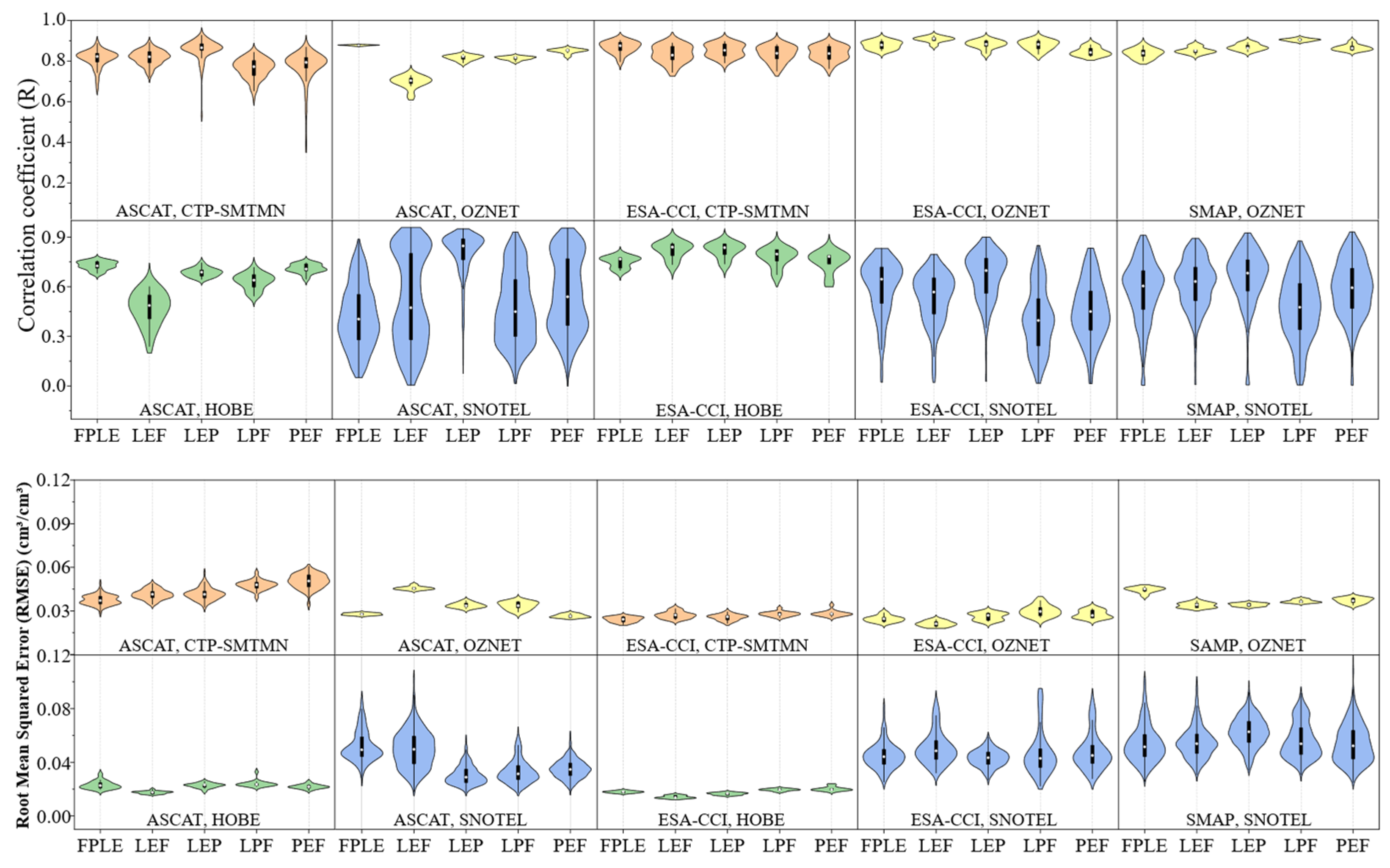
Analysis of the SM improvement effect based on different satellite data showed that the performance of the MLSTM SM framework was affected by the network space range of the site and the combination of variables. In the violin plots of RMSE and R values for different combinations of networks and variables (Figure 9), the SNOTEL network performs poorly in key indicators of model evaluation, with the largest interquartile range between the RMSE and R values (RMSE up to 0.02 cm³/cm³ and R up to 0.5), indicating that the model’s performance is not yet very stable over a large spatial range. In the estimation at the site scale, there are significant differences in the performance of different variable combination models. The FPLE variable combination, as an estimation model with all variables input, performs the most stably and performs the best in both the OZNET and HOBE networks. In the CTP–SMTMN and SNOTEL networks, after removing the vegetation coverage variable from the FPLE variable combination, the R values of the estimation model based on the ASCAT grid increased by 0.055 and 0.025, respectively, and the R values of the estimation model based on the ESA–CCI grid increased by 0.010 and 0.011, respectively, indicating that the variable combinations adapted to different regions are different.

Overall, the MLSTM proposed in this study showed significant improvement on the ASCAT, ESA–CCI, and SMAP SM products in different observation network regions, and the optimization results were more prominent in the ASCAT product, demonstrating a certain degree of universality and providing a potential way for the optimization of satellite SM products.

References

1. Zhang, Q.; Fan, K.; Singh, V.P.; Song, C.; Xu, C.Y.; Sun, P. Is Himalayan-Tibetan Plateau “drying”? Historical estimations and future trends of surface soil moisture. Sci. Total Environ. 2019, 658, 374–384. [Google Scholar] [CrossRef] [PubMed]
2. Bormann, H. Assessing the soil texture-specific sensitivity of simulated soil moisture to projected climate change by SVAT modelling. Geoderma 2012, 185–186, 73–83. [Google Scholar] [CrossRef]
3. Wagner, W.; Hahn, S.; Kidd, R.; Melzer, T.; Bartalis, Z.; Hasenauer, S.; Figa-Saldaña, J.; de Rosnay, P.; Jann, A.; Schneider, S.; et al. The ASCAT Soil Moisture Product: A Review of its Specifications, Validation Results, and Emerging Applications. Meteorol. Z. 2013, 22, 5–33. [Google Scholar] [CrossRef]
4. Dostálová, A.; Doubková, M.; Sabel, D.; Bauer-Marschallinger, B.; Wagner, W. Seven Years of Advanced Synthetic Aperture Radar (ASAR) Global Monitoring (GM) of Surface Soil Moisture over Africa. Remote Sens. 2014, 6, 7683–7707. [Google Scholar] [CrossRef]
5. Entekhabi, D.; Njoku, E.G.; O’Neill, P.E.; Kellogg, K.H.; Crow, W.T.; Edelstein, W.N.; Entin, J.K.; Goodman, S.D.; Jackson, T.J.; Johnson, J.; et al. The Soil Moisture Active Passive (SMAP) Mission. Proc. IEEE 2010, 98, 704–716. [Google Scholar] [CrossRef]
6. Dorigo, W.A.; Gruber, A.; De Jeu, R.A.M.; Wagner, W.; Stacke, T.; Loew, A.; Albergel, C.; Brocca, L.; Chung, D.; Parinussa, R.M.; et al. Evaluation of the ESA CCI soil moisture product using ground-based observations. Remote Sens. Environ. 2015, 162, 380–395. [Google Scholar] [CrossRef]
7. Gruber, A.; Su, C.H.; Zwieback, S.; Crow, W.; Dorigo, W.; Wagner, W. Recent advances in (soil moisture) triple collocation analysis. Int. J. Appl. Earth Obs. Geoinf. 2016, 45, 200–211. [Google Scholar] [CrossRef]
8. Colliander, A.; Jackson, T.J.; Bindlish, R.; Chan, S.; Das, N.; Kim, S.B.; Cosh, M.H.; Dunbar, R.S.; Dang, L.; Pashaian, L.; et al. Validation of SMAP surface soil moisture products with core validation sites. Remote Sens. Environ. 2017, 191, 215–231. [Google Scholar] [CrossRef]
9. Al-Yaari, A.; Wigneron, J.P.; Dorigo, W.; Colliander, A.; Pellarin, T.; Hahn, S.; Mialon, A.; Richaume, P.; Fernandez-Moran, R.; Fan, L.; et al. Assessment and inter-comparison of recently developed/reprocessed microwave satellite soil moisture products using ISMN ground-based measurements. Remote Sens. Environ. 2019, 224, 289–303. [Google Scholar] [CrossRef]
10. Colliander, A.; Reichle, R.H.; Crow, W.T.; Cosh, M.H.; Chen, F.; Chan, S.; Das, N.N.; Bindlish, R.; Chaubell, J.; Kim, S.; et al. Validation of Soil Moisture Data Products From the NASA SMAP Mission. IEEE J. Sel. Top. Appl. Earth Obs. Remote Sens. 2022, 15, 364–392. [Google Scholar] [CrossRef]
11. Zheng, J.; Zhao, T.; Lü, H.; Shi, J.; Cosh, M.H.; Ji, D.; Jiang, L.; Cui, Q.; Lu, H.; Yang, K.; et al. Assessment of 24 soil moisture datasets using a new in situ network in the Shandian River Basin of China. Remote Sens. Environ. 2022, 271, 112891. [Google Scholar] [CrossRef]
12. Kim, H.; Crow, W.; Li, X.; Wagner, W.; Hahn, S.; Lakshmi, V. True global error maps for SMAP, SMOS, and ASCAT soil moisture data based on machine learning and triple collocation analysis. Remote Sens. Environ. 2023, 298, 113776. [Google Scholar] [CrossRef]
13. Xu, L.; Chen, N.; Zhang, X.; Moradkhani, H.; Zhang, C.; Hu, C. In-situ and triple-collocation based evaluations of eight global root zone soil moisture products. Remote Sens. Environ. 2021, 254, 112248. [Google Scholar] [CrossRef]
14. Zhang, J.; Becker-Reshef, I.; Justice, C. Evaluation of the ASCAT surface soil moisture product for agricultural drought monitoring in USA. In Proceedings of the 2015 IEEE International Geoscience and Remote Sensing Symposium (IGARSS), Milan, Italy, 26–31 July 2015; pp. 669–672. [Google Scholar]
15. Kim, H.; Parinussa, R.; Konings, A.G.; Wagner, W.; Cosh, M.H.; Lakshmi, V.; Zohaib, M.; Choi, M. Global-scale assessment and combination of SMAP with ASCAT (active) and AMSR2 (passive) soil moisture products. Remote Sens. Environ. 2018, 204, 260–275. [Google Scholar] [CrossRef]
16. Ding, T.; Zhao, W.; Yang, Y. Addressing spatial gaps in ESA CCI soil moisture product: A hierarchical reconstruction approach using deep learning model. Int. J. Appl. Earth Obs. Geoinf. 2024, 132, 104003. [Google Scholar] [CrossRef]
17. Liu, P.W.; Judge, J.; Roo, R.D.D.; England, A.W.; Bongiovanni, T. Uncertainty in Soil Moisture Retrievals Using the SMAP Combined Active–Passive Algorithm for Growing Sweet Corn. IEEE J. Sel. Top. Appl. Earth Obs. Remote Sens. 2016, 9, 3326–3339. [Google Scholar] [CrossRef]
18. Crow, W.T.; Berg, A.A.; Cosh, M.H.; Loew, A.; Mohanty, B.P.; Panciera, R.; de Rosnay, P.; Ryu, D.; Walker, J.P. Upscaling sparse ground-based soil moisture observations for the validation of coarse-resolution satellite soil moisture products. Rev. Geophys. 2012, 50, RG2002. [Google Scholar] [CrossRef]
19. Meng, X.; Li, R.; Luan, L.; Lyu, S.; Zhang, T.; Ao, Y.; Han, B.; Zhao, L.; Ma, Y. Detecting hydrological consistency between soil moisture and precipitation and changes of soil moisture in summer over the Tibetan Plateau. Clim. Dyn. 2017, 51, 4157–4168. [Google Scholar] [CrossRef]
20. Wang, J.; Xu, D. Artificial Neural Network-Based Microwave Satellite Soil Moisture Reconstruction over the Qinghai–Tibet Plateau, China. Remote Sens. 2021, 13, 5156. [Google Scholar] [CrossRef]
21. Berg, A.; Sheffield, J.; Milly, P.C.D. Divergent surface and total soil moisture projections under global warming. Geophys. Res. Lett. 2017, 44, 236–244. [Google Scholar] [CrossRef]
22. Mao, L.; Pei, X.; He, C.; Bian, P.; Song, D.; Fang, M.; Wu, W.; Zhan, H.; Zhou, W.; Tian, G. Spatiotemporal Changes in Vegetation Cover and Soil Moisture in the Lower Reaches of the Heihe River Under Climate Change. Forests 2024, 15, 1921. [Google Scholar] [CrossRef]
23. Rasheed, M.W.; Tang, J.; Sarwar, A.; Shah, S.; Saddique, N.; Khan, M.U.; Imran Khan, M.; Nawaz, S.; Shamshiri, R.R.; Aziz, M.; et al. Soil Moisture Measuring Techniques and Factors Affecting the Moisture Dynamics: A Comprehensive Review. Sustainability 2022, 14, 11538. [Google Scholar] [CrossRef]
24. Kwon, M.; Han, D. Assessment of remotely sensed soil moisture products and their quality improvement: A case study in South Korea. J. Hydro-Environ. Res. 2019, 24, 14–27. [Google Scholar] [CrossRef]
25. Zhu, Q.; Wang, Y.; Luo, Y. Improvement of multi-layer soil moisture prediction using support vector machines and ensemble Kalman filter coupled with remote sensing soil moisture datasets over an agriculture dominant basin in China. Hydrol. Process. 2021, 35, e14154. [Google Scholar] [CrossRef]
26. Cui, K.; Xing, M.; Shang, J.; Zhou, X.; Wang, J. Enhanced L-MEB Model for Soil Moisture Retrieval Over Soybean Fields During the Growing Season. IEEE Trans. Geosci. Remote Sens. 2025, 63, 4409216. [Google Scholar] [CrossRef]
27. Hagan, D.F.T.; Kim, S.; Wang, G.; Ma, X.; Hu, Y.; Liu, Y.Y.; Barth, A.; Liu, H.; Ullah, W.; Nooni, I.K.; et al. Seamless finer-resolution soil moisture from the synergistic merging of the FengYun-3 satellite series. Sci. Data 2025, 12, 983. [Google Scholar] [CrossRef] [PubMed]
28. Li, S.; Xing, M.; Dong, T. An Apparent Thermal Inertia Based Trapezoid Model for Downscaling ESA CCI Soil Moisture Products. IEEE J. Sel. Top. Appl. Earth Obs. Remote Sens. 2025, 18, 4473–4486. [Google Scholar] [CrossRef]
29. Zhao, H.; Zhao, H.; Zhang, C. Validating Data Interpolation Empirical Orthogonal Functions Interpolated Soil Moisture Data in the Contiguous United States. Agriculture 2025, 15, 1212. [Google Scholar] [CrossRef]
30. Jin, M.; Zheng, X.; Jiang, T.; Li, X.; Li, X.-J.; Zhao, K. Evaluation and Improvement of SMOS and SMAP Soil Moisture Products for Soils with High Organic Matter over a Forested Area in Northeast China. Remote Sens. 2017, 9, 387. [Google Scholar] [CrossRef]
31. Guo, X.; Fang, X.; Cao, Y.; Yang, L.; Ren, L.; Chen, Y.; Zhang, X. Reconstruction of ESA CCI soil moisture based on DCT-PLS and in situ soil moisture. Hydrol. Res. 2022, 53, 1221–1236. [Google Scholar] [CrossRef]
32. Yin, J.; Zhan, X.; Barlage, M.; Liu, J.; Meng, H.; Ferraro, R.R. Refinement of NOAA AMSR-2 Soil Moisture Data Product—Part 2: Development With the Optimal Machine Learning Model. IEEE Trans. Geosci. Remote Sens. 2023, 61, 4405311. [Google Scholar] [CrossRef]
33. Cui, Y.; Yang, X.; Chen, X.; Fan, W.; Zeng, C.; Xiong, W.; Hong, Y. A two-step fusion framework for quality improvement of a remotely sensed soil moisture product: A case study for the ECV product over the Tibetan Plateau. J. Hydrol. 2020, 587, 124993. [Google Scholar] [CrossRef]
34. Liu, Y.Y.; Parinussa, R.M.; Dorigo, W.A.; De Jeu, R.A.M.; Wagner, W.; van Dijk, A.I.J.M.; McCabe, M.F.; Evans, J.P. Developing an improved soil moisture dataset by blending passive and active microwave satellite-based retrievals. Hydrol. Earth Syst. Sci. 2011, 15, 425–436. [Google Scholar] [CrossRef]
35. Jordan, M.I.; Mitchell, T.M. Machine learning: Trends, perspectives, and prospects. Science 2015, 349, 255–260. [Google Scholar] [CrossRef] [PubMed]
36. Jiang, M.; Qiu, T.; Wang, T.; Zeng, C.; Zhang, B.; Shen, H. Seamless global daily soil moisture mapping using deep learning based spatiotemporal fusion. Int. J. Appl. Earth Obs. Geoinf. 2025, 139, 104517. [Google Scholar] [CrossRef]
37. Nasiri Khiavi, A. Application of remote sensing indicators and deep learning algorithms to model the spatial distribution of soil moisture. Earth Sci. Inform. 2025, 18, 404. [Google Scholar] [CrossRef]
38. Xu, N.; Andre, D.; Arman, A.; Derek, H.; Perez-Barquero, F.P. Soil moisture estimation with microwave remote sensing: A systematic review and meta-analysis. Int. J. Digit. Earth 2025, 18, 1–27. [Google Scholar] [CrossRef]
39. Cui, Y.; Long, D.; Hong, Y.; Zeng, C.; Zhou, J.; Han, Z.; Liu, R.; Wan, W. Validation and reconstruction of FY-3B/MWRI soil moisture using an artificial neural network based on reconstructed MODIS optical products over the Tibetan Plateau. J. Hydrol. 2016, 543, 242–254. [Google Scholar] [CrossRef]
40. Fang, K.; Shen, C.; Kifer, D.; Yang, X. Prolongation of SMAP to Spatiotemporally Seamless Coverage of Continental U.S. Using a Deep Learning Neural Network. Geophys. Res. Lett. 2017, 44, 11030–11039. [Google Scholar] [CrossRef]
41. Fang, K.; Pan, M.; Shen, C. The Value of SMAP for Long-Term Soil Moisture Estimation With the Help of Deep Learning. IEEE Trans. Geosci. Remote Sens. 2019, 57, 2221–2233. [Google Scholar] [CrossRef]
42. Roberts, T.M.; Colwell, I.; Chew, C.; Lowe, S.; Shah, R. A Deep-Learning Approach to Soil Moisture Estimation with GNSS-R. Remote Sens. 2022, 14, 3299. [Google Scholar] [CrossRef]
43. Abebe, A.K.; Zhou, X.; Lv, T.; Tao, Z.; Elnashar, A.; Kebede, A.; Wang, C.; Zhang, H. Spatial Downscaling of Soil Moisture Product to Generate High-Resolution Data: A Multi-Source Approach over Heterogeneous Landscapes in Kenya. Remote Sens. 2025, 17, 1763. [Google Scholar] [CrossRef]
44. Taheri, M.; Bigdeli, M.; Imanian, H.; Mohammadian, A. An Overview of Machine-Learning Methods for Soil Moisture Estimation. Water 2025, 17, 1638. [Google Scholar] [CrossRef]
45. Zhang, L.; Liu, Y.; Ren, L.; Teuling, A.J.; Zhang, X.; Jiang, S.; Yang, X.; Wei, L.; Zhong, F.; Zheng, L. Reconstruction of ESA CCI satellite-derived soil moisture using an artificial neural network technology. Sci. Total Environ. 2021, 782, 146602. [Google Scholar] [CrossRef]
46. Hu, Y.; Wang, G.; Wei, X.; Zhou, F.; Kattel, G.; Amankwah, S.O.Y.; Hagan, D.F.T.; Duan, Z. Reconstructing long-term global satellite-based soil moisture data using deep learning method. Front. Earth Sci. 2023, 11, 1130853. [Google Scholar] [CrossRef]
47. Cai, G.; Xue, Y.; Hu, Y.; Wang, Y.; Guo, J.; Luo, Y.; Wu, C.; Zhong, S.; Qi, S. Soil moisture retrieval from MODIS data in Northern China Plain using thermal inertia model. Int. J. Remote Sens. 2007, 28, 3567–3581. [Google Scholar] [CrossRef]
48. Yang, K.; Qin, J.; Zhao, L.; Chen, Y.; Tang, W.; Han, M.; Lazhu; Chen, Z.; Lv, N.; Ding, B.; et al. A Multiscale Soil Moisture and Freeze–Thaw Monitoring Network on the Third Pole. Bull. Am. Meteorol. Soc. 2013, 94, 1907–1916. [Google Scholar] [CrossRef]
49. Jensen, K.H.; Refsgaard, J.C. HOBE: The Danish Hydrological Observatory. Vadose Zone J. 2018, 17, 1–24. [Google Scholar] [CrossRef]
50. Smith, A.B.; Walker, J.P.; Western, A.W.; Young, R.I.; Ellett, K.M.; Pipunic, R.C.; Grayson, R.B.; Siriwardena, L.; Chiew, F.H.S.; Richter, H. The Murrumbidgee soil moisture monitoring network data set. Water Resour. Res. 2012, 48, W07701. [Google Scholar] [CrossRef]
51. Albergel, C.; Rüdiger, C.; Pellarin, T.; Calvet, J.C.; Fritz, N.; Froissard, F.; Suquia, D.; Petitpa, A.; Piguet, B.; Martin, E. From near-surface to root-zone soil moisture using an exponential filter: An assessment of the method based on in-situ observations and model simulations. Hydrol. Earth Syst. Sci. 2008, 12, 1323–1337. [Google Scholar] [CrossRef]
52. Wagner, W.; Lemoine, G.; Rott, H. A Method for Estimating Soil Moisture from ERS Scatterometer and Soil Data. Remote Sens. Environ. 1999, 70, 191–207. [Google Scholar] [CrossRef]
53. Entekhabi, D.; Reichle, R.H.; Koster, R.D.; Crow, W.T. Performance Metrics for Soil Moisture Retrievals and Application Requirements. J. Hydrometeorol. 2010, 11, 832–840. [Google Scholar] [CrossRef]
54. Dorigo, W.; Wagner, W.; Albergel, C.; Albrecht, F.; Balsamo, G.; Brocca, L.; Chung, D.; Ertl, M.; Forkel, M.; Gruber, A.; et al. ESA CCI Soil Moisture for improved Earth system understanding: State-of-the art and future directions. Remote Sens. Environ. 2017, 203, 185–215. [Google Scholar] [CrossRef]
55. Jia, K.; Yang, L.; Liang, S.; Xiao, Z.; Zhao, X.; Yao, Y.; Zhang, X.; Jiang, B.; Liu, D. Long-Term Global Land Surface Satellite (GLASS) Fractional Vegetation Cover Product Derived From MODIS and AVHRR Data. IEEE J. Sel. Top. Appl. Earth Obs. Remote Sens. 2019, 12, 508–518. [Google Scholar] [CrossRef]
56. Zhao, T.; Yu, P. Global Daily 0.05° Spatiotemporal Continuous Land Surface Temperature Dataset (2002–2020). 2021. Available online: https://cstr.cn/18406.11.Meteoro.tpdc.271663 (accessed on 21 March 2025).
57. Huffman, G.J.; Stocker, E.F.; Bolvin, D.T.; Nelkin, E.J.; Tan, J. GPM IMERG Final Precipitation L3 1 Day 0.1 Degree × 0.1 Degree V07. 2024. Available online: https://rda.ucar.edu/datasets/d734000/ (accessed on 23 March 2025).
58. Jiao, L.; Guojie, W.; Tiexi, C.; Shijie, L.; Daniel, H.; Giri, K.; Jian, P.; Tong, J.; Buda, S. A Harmonized Global Land Evaporation Dataset from Model-Based Products Covering 1980–2017. 2021. Available online: https://zenodo.org/records/4595941 (accessed on 23 March 2025).
59. Dorigo, W.A.; Xaver, A.; Vreugdenhil, M.; Gruber, A.; Hegyiová, A.; Sanchis-Dufau, A.D.; Zamojski, D.; Cordes, C.; Wagner, W.; Drusch, M. Global Automated Quality Control of In Situ Soil Moisture Data from the International Soil Moisture Network. Vadose Zone J. 2013, 12, 918–924. [Google Scholar] [CrossRef]
60. Xie, Q.; Jia, L.; Menenti, M.; Chen, Q.; Bi, J.; Chen, Y.; Wang, C.; Yu, X. Evaluation of remote sensing soil moisture data products with a new approach to analyse footprint mismatch with in-situ measurements. Int. J. Digit. Earth 2024, 17, 2437051. [Google Scholar] [CrossRef]
61. Hochreiter, S.; Schmidhuber, J. Long Short-Term Memory. Neural Comput. 1997, 9, 1735–1780. [Google Scholar] [CrossRef] [PubMed]
62. Lundberg, S.M.; Lee, S.-I. A unified approach to interpreting model predictions. In Proceedings of the 31st International Conference on Neural Information Processing Systems, Long Beach, CA, USA, 4–9 December 2017; pp. 4768–4777. [Google Scholar]
63. Fathololoumi, S.; Vaezi, A.R.; Firozjaei, M.K.; Biswas, A. Quantifying the effect of surface heterogeneity on soil moisture across regions and surface characteristic. J. Hydrol. 2021, 596, 126132. [Google Scholar] [CrossRef]
64. Yongqiang, C.; Na, Y.; Xin, H.; Mingyuan, T. Study on Stability of Surface Soil Moisture during SMOS and SMAP Transit period. Remote Sens. Technol. Appl. 2020, 35, 58–64. [Google Scholar] [CrossRef]
65. Deng, Q.; Yang, J.; Zhang, L.; Sun, Z.; Sun, G.; Chen, Q.; Dou, F. Analysis of Seasonal Driving Factors and Inversion Model Optimization of Soil Moisture in the Qinghai Tibet Plateau Based on Machine Learning. Water 2023, 15, 2859. [Google Scholar] [CrossRef]
66. Rooney, E.C.; Bailey, V.L.; Patel, K.F.; Possinger, A.R.; Gallo, A.C.; Bergmann, M.; Lybrand, R. The Impact of Freeze-Thaw History on Soil Carbon Response to Experimental Freeze-Thaw Cycles. J. Geophys. Res. Biogeosci. 2022, 127, e2022JG006889. [Google Scholar] [CrossRef]
67. Kumar, S.V.; Peters-Lidard, C.D.; Santanello, J.A.; Reichle, R.H.; Draper, C.S.; Koster, R.D.; Nearing, G.; Jasinski, M.F. Evaluating the utility of satellite soil moisture retrievals over irrigated areas and the ability of land data assimilation methods to correct for unmodeled processes. Hydrol. Earth Syst. Sci. 2015, 19, 4463–4478. [Google Scholar] [CrossRef]
68. Xiong, Z.; Zhang, Z.; Gui, H.; Chen, X.; Hu, S.; Gao, L.; Yang, H.; Qiu, J.; Xin, Q. A Meteorology-Driven Transformer Network to Predict Soil Moisture for Agriculture Drought Forecasting. IEEE Trans. Geosci. Remote Sens. 2025, 63, 4405818. [Google Scholar] [CrossRef]
Figure 1. Flowchart for correction of global-scale ASCAT, SMAP, and ESA–CCI SM datasets.
Remotesensing 17 02456 g001
Figure 2. Distribution of in-situ measurement networks (HOBE, CTP–SMTMN, OZNET, and SNOTEL).
Remotesensing 17 02456 g002
Figure 3. LSTM hidden layer unit diagram ( x t : input vector at timestep t; C t 1 and C t : previous moment and updated cell state; h t 1 and h t : previous moment and updated hidden state; f t : forget gate output; i t : input gate output; C ~ i : candidate cell state; o t : output gate output; σ : sigmoid activation function; t a n h : hyperbolic tangent activation function; ⊗: element-wise multiplication; ⊕: element-wise summation).
Remotesensing 17 02456 g003
Figure 4. The multi-source long short-term memory (MLSTM) algorithm for the correction of ASCAT, SMAP and ESA–CCI soil moisture products soil moisture (ET: Evapotranspiration; LST: Land Surface Temperature; FVC: Fractional Vegetation Cover; RPE: Precipitation; x t 1 , x t and x t + 1 : input vector at timestep t 1 , t and t + 1 ; h t 1 , h t and h t + 1 : output at timestep t 1 , t and t + 1 ; C t 1 , C t and C t + 1 : cell state at timestep t 1 , t and t + 1 ).
Remotesensing 17 02456 g004
Figure 5. Temporal evolutions of precipitation (PRE), surface temperature (LST), vegetation coverage (FVC), evapotranspiration (ET), and in-site SM measurements of the CTP–SMTMN, HOBE, OZNET, and SNOTEL observation networks.
Remotesensing 17 02456 g005aRemotesensing 17 02456 g005b
Figure 6. Scatter plots of the estimated in-situ SM matching ASCAT, ESA–CCI, and SMAP product grids at five variable combinations (i.e., FPLE, LEF, LEP, LPF and PEF), and in-site measured SM data of HOBE, OZNET, CTP–SMTMN, and SNOTEL networks. ( n represents the number of samples used for drawing the scatter plot).
Remotesensing 17 02456 g006aRemotesensing 17 02456 g006b
Figure 7. Temporal evolution plots of the estimated in-situ SM matching ASCAT (0.1°), ESA–CCI (0.25°), and SMAP (0.1°) product grids at five variable combinations (i.e., FPLE, LEF, LEP, LPF, and PEF), and in-situ measured SM data of HOBE, OZNET, CTP–SMTMN, and SNOTEL networks.
Remotesensing 17 02456 g007aRemotesensing 17 02456 g007b
Figure 8. SHAP summary plots (ad) represent HOBE, OZNET, CTP–SMTMN, and SNOTEL networks, respectively, and (15) represent combinations: FVC, PRE, LST, and ET, respectively; LST, ET, FVC; LST, ET, PRE; LST, PRE, FVC; and PRE, ET, FVC).
Remotesensing 17 02456 g008
Figure 9. RMSE and R violin plots of ASCAT, ESA–CCI, SAMP, and estimated in-situ SM data under five variable combinations (FPLE: FVC, PRE, LST, and ET; LEF: LST, ET, and FVC; LEP: LST, ET, and PER; LPF: LST, PRE, and FVC; PEF: PRE, ET, and FVC) in four in-situ observation networks (HOBE, OZNET, CTP–SMTMN, and SNOTEL).
Remotesensing 17 02456 g009
Figure 10. Comparison of original and improved ASCAT, ESA–CCI, and SMAP products (9 September 2016) in areas of CTP–SMTMN, OZNET, HOBE, and SNOTEL observation networks.
Remotesensing 17 02456 g010
Figure 11. Taylor diagrams of the improved and original ASCAT, ESA–CCI, and SMAP SM data products against in-situ SM measurements of CTP–SMTMN, HOBE, OZNET, and SNOTEL networks under five variable combinations i.e., FPLE (FVC, PRE, LST, and ET), LEF (LST, ET, and FVC), LEP (LST, ET, and PER), LPF (LST, PRE, and FVC), PEF (PRE, ET, and FVC). The red dotted line represents the indicator Root Mean-Square Deviation (RMSD).
Remotesensing 17 02456 g011