Soil Moisture Prediction Using the VIC Model Coupled with LSTMseq2seq

Abstract

Soil moisture (SM) is a key variable in agricultural ecosystems and is crucial for drought prevention and control management. However, SM is influenced by underlying surface and meteorological conditions, and it changes rapidly in time and space. To capture the changes in SM and improve the accuracy of short-term and medium-to-long-term predictions on a daily scale, an LSTMseq2seq model driven by both observational data and mechanism models was constructed. This framework combines historical meteorological elements and SM, as well as the SM change characteristics output by the VIC model, to predict SM over a 90-day period. The model was validated using SMAP SM. The proposed model can accurately predict the spatiotemporal variations in SM in Jiangxi Province. Compared with classical machine learning (ML) models, traditional LSTM models, and advanced transformer models, the LSTMseq2seq model achieved R² values of 0.949, 0.9322, 0.8839, 0.8042, and 0.7451 for the prediction of surface SM over 3 days, 7 days, 30 days, 60 days, and 90 days, respectively. The mean absolute error (MAE) ranged from 0.0118 m³/m³ to 0.0285 m³/m³. This study also analyzed the contributions of meteorological features and simulated future SM state changes to SM prediction from two perspectives: time importance and feature importance. The results indicated that meteorological and SM changes within a certain time range prior to the prediction have an impact on SM prediction. The dual-driven LSTMseq2seq model has unique advantages in predicting SM and is conducive to the integration of physical mechanism models with data-driven models for handling input features of different lengths, providing support for daily-scale SM time series prediction and drought dynamics prediction.

1. Introduction

Drought has been one of the most negatively impactful natural disasters in the past few decades, often triggering food crises and irreversible damage to ecosystems and causing huge socio-economic losses [1]. Against the backdrop of global warming, extreme climate phenomena have intensified, further exacerbating these negative impacts, and the defense against drought has received widespread attention. Soil moisture (SM) is an important component of the global water cycle system [2] and is widely used in drought assessment, playing a key role in it [3]. Large-scale, long-term series and high-precision SM prediction has significant scientific value and strategic significance for regional and even global climate change research, water cycle analysis, vegetation status monitoring, and drought and flood early warning [4,5]. Accurate SM prediction has played a significant role in formulating irrigation systems and drought prevention and resistance measures [6]. In soil and environmental management applications, it is usually necessary to conduct SM prediction one month in advance. SM is affected by various factors such as precipitation, soil properties and topography [7,8], making SM prediction both deterministic and obviously nonlinear, and making accurate prediction complex. The commonly used SM simulation methods mainly include remote sensing technology, mechanism model simulation, and machine learning (ML) models.

Remote sensing technology makes up for shortcomings in the spatial coverage of site monitoring, can provide a wide range of SM results, and has a high temporal and spatial resolution. In recent years, multiple SM observation satellites have been launched successively, for example the Advanced Microwave Scanning Radiometer for Earth Observing System (AMSR-E), Soil Moisture Ocean Salinity (SMOS), and Soil Moisture Active and Passive (SMAP). These satellites provide long-term and global SM, offering significant support for global agricultural drought prediction [9,10]. Among these data, the SMAP SM product has excellent performance and a high temporal resolution, providing reliable SM information worldwide [11]. Its superiority has been widely validated [10,12]. In real-world application, the overall accuracy of SMAP products is superior to that of AMSR2 products. The SM state is jointly affected by dynamic surface parameters and static underlying surfaces. However, remote sensing technology is still limited to surface measurement (<5 cm), is hindered by vegetation interference, and is mainly focused on monitoring.

The mechanism model is a method used to predict the changes in SM. Over the past few decades, many scholars have attempted to predict SM using control equations based on complex hydrological processes [13,14]. With the development of technology, the use of hydrological models has become widespread, and the reliability of these models has been confirmed [15]. The VIC model can take into account factors such as soil texture, vegetation coverage and climatic conditions, and can obtain continuous spatiotemporal sequences of SM. It is widely used in SM simulation [16,17]. Other models used to simulate SM also include SWAP, SWAT, and HYDRUS. The selection of a model depends on the simulation’s purpose, spatial resolution, model complexity and available parameter information [18]. However, due to the unclear mechanisms of each link from rainfall to SM transport, a large number of parameters of the model need to be generalized, reducing the accuracy of simulation [19,20].

In recent years, ML has developed rapidly. Some studies have evaluated the performance and limitations of physical models and explored ML models as alternatives [21,22]. Research shows that models based on artificial intelligence can outperform those based on physics, demonstrating significant value [23,24]. ML methods are widely used to estimate SM [25,26]. Traditional ML methods, such as random forest (RF), multiple linear regression (MLR), support vector machine (SVM), and gradient boosting regression tree (GBRT), provide effective approaches for SM prediction, fully demonstrating the application potential of ML in this field [27,28]. The hourly SM in Taichung area, Taiwan, was predicted using the RF by Chen et al. [29]. Li et al., in 2024 [30], improved global SM prediction based on the meta-learning model using the Koppen–Geigel climate classification. This rapidly developing deep learning (DL) technology also provides an effective approach for understanding data-driven Earth system science [31] and establishing nonlinear relationships between model inputs and outputs. A large number of studies have shown that the correlation between the predictions and measured values of artificial neural network (ANN) models is good [32]. The DL models can take dynamic climate variables and surface features as inputs to predict SM [33]. DL models commonly used for predicting SM include ANNs, deep neural networks (DNNs), recurrent neural networks (RNNs), and long short-term memory (LSTM) [34]. ANNs provide new opportunities to estimate global SM through learning a generative model from a series of available SM products. In recent years, the classic shallow ANN has been successfully applied for SMOS and SMAP SM retrievals. Gao et al., in 2022 [33], presented a DNN that combines the advantages of a suite of existing satellite and reanalysis products to produce a new SM product with minimum (maximum) bias (correlation), using NASA’s SMAP data and ERA5 reanalysis. In 2024, Zhao et al. [35] compared the performance of an RNN and a CNN in hydrological prediction. Transformer-based models have shown remarkable capabilities in improving the accuracy of SM prediction [36]. Furthermore, studies have shown that LSTM demonstrates superior performance [37]. LSTM is a type of time-recurrent neural network specifically designed to address the long-term dependency issue that exists in general RNNs. All RNNs have a chain-like form of repetitive neural network modules. The improved and derived methods based on LSTM have effectively enhanced the accuracy in SM simulation and prediction [38]. They can predict the SM changes in the next month and perform well in predicting meteorological droughts in the next three months; they are also capable of issuing drought warnings 5 to 7 days in advance.

The memory characteristics of SM at different time scales have different influences on long-term SM prediction in data-driven models [39]. Although LSTM excels in capturing long-term correlations [21], its original design is mainly based on historical information rather than the overall time series when predicting individual future time points, which may make it difficult for the model to fully mine or appropriately allocate key information in long-term data analysis. Encoder–decoder architecture and location coding can effectively handle complex patterns in meteorological data, thereby improving the accuracy of deterministic prediction and extreme weather prediction. The encoder–decoder model shows significant potential in predicting Earth system processes such as SM time series and agricultural drought. Li et al. [40] proposed a multi-step SM prediction model based on spatio-temporal deep encoder–decoder networks, demonstrating its adaptability to different climate regions. Li et al. [41] proposed a novel SM prediction model, REDF-LSTM, and enhanced the model’s ability to capture complex nonlinear relationships.

SM is influenced by multiple factors such as precipitation, radiation, temperature, humidity, wind speed, land cover, and soil properties, and has memory for historical data. These relationships are usually nonlinear, so predicting SM is particularly challenging. The selection of both models and data is very important. Some achievements have been made in this area of research. The research suggests that meteorological factors have the greatest impact on SM prediction [42], and that previous and current SM has an influence on estimating future SM [43]. Yu et al. [44] established the ResBiLSTM SM prediction model using grid meteorological data and SM. Multiple variables, including soil temperature, relative humidity, temperature, total radiation and evapotranspiration, were used as ML inputs to improve the accuracy of SM prediction at different depths. Considering historical and meteorological data for SM prediction in the ML model can better improve the accuracy of SM prediction. Fedasyuk and Kostiuk [45] used historical data and weather forecast data to develop ML models for SM prediction. This coupled modeling method combines process-based models with AI-based ML techniques, providing enhanced predictive performance [46]. Coupling mechanism models with ML has become a research hotspot. A large number of studies have shown that the coupling of mechanism models with ML has significant advantages for mining and capturing complex meteorological, hydrological and underlying surface features to improve the prediction ability of SM, providing a new technical path for hydrological simulation. Zhao et al. [47] significantly improved the accuracy of SM simulation by enhancing the parameterization scheme of the land surface process model (LSM) and combining it with ML techniques.

Remote sensing, mechanism models and ML each have their advantages in SM monitoring and prediction, but they also have limitations. At present, there are relatively few studies on SM prediction models that combine these three methods. Commonly used DL models (such as LSTM) and ML models require regular matrix input and are often constructed by data dimensionality reduction or feature information reduction. There are relatively few studies on multi-step prediction models of daily-scale SM with time dependence, different feature lengths and different quantities. In this study, a VIC-LSTMseq2seq model was constructed. The input included the meteorological and SM from the past N days, as well as the meteorological data and VIC model simulation results for the next M days. The SM on the M day in the future was predicted, and it was compared with that of classical ML models, classic DL models such as the LSTM model, and the advanced transformer model. The key points of innovation in this research include the following: (1) we integrated physical mechanisms and DL, comprehensively considering the characteristics of the past and the future; (2) the model we constructed can handle feature inputs of different lengths and quantities, taking into account the SM memory; (3) this research explains the model’s behavior through feature importance analysis and identifies the main influencing factors. This research is innovative in its design of the coupled model and performance validation, and contributes to improving prediction accuracy.

2. Materials and Methods

2.1. Study Area

The study area is located in Jiangxi province (Figure 1), which is situated on the south bank of the middle and lower reaches of the Yangtze River and encompasses the Poyang Lake Basin. Poyang Lake Basin covers 94% of Jiangxi’s area and forms a relatively complete basin. As the largest freshwater lake basin in China and an important ecological functional area, the Poyang Lake Basin, as a typical representative of the subtropical monsoon climate zone, has unique SM dynamics that are of significant research value, which is mainly reflected by the following: (1) as a key hydrological node in the middle reaches of the Yangtze River, changes in SM within the basin directly affect the water level fluctuations of Poyang Lake and the wetland ecosystem; (2) the complex topography (elevation ranging from approximately −20 to 2157 m) forms a complete SM gradient belt from the lakeside plain to the hilly and mountainous areas; (3) the distinct seasonal alternation of wet and dry periods provides an ideal setting for studying SM responses under climate change. As an important water regulator in the middle reaches of the Yangtze River, changes in SM in the Poyang Lake Basin are directly related to regional water resource security, the maintenance of the Poyang Lake wetland ecosystem, and the carbon cycling process. The unique “river–lake relationship” and its impact on SM dynamics make it a typical representative for studying SM cycling in monsoon regions. Under the background of global change, SM simulation research in this basin is not only of great significance for regional agricultural drought resistance and disaster reduction but also provides a scientific basis for ecological security early warning in the Yangtze River economic belt.

Jiangxi Province has distinct topographical features, with a complete landscape sequence from lakeside plains and ridges to surrounding hilly and mountainous areas. This gradient variation leads to the significant spatial heterogeneity of SM. The climate is characterized by warm and rainy springs, hot and humid summers, cool and less rainy autumns, and cold and dry winters. The average annual precipitation is 1638 mm, and the average annual terrestrial evaporation in most areas ranges from 700 to 800 mm, while the average annual water surface evaporation ranges from 800 to 1200 mm. The climatic characteristics are as follows: spring (March–May) is the rapid recovery period for SM (average temperature 17.3 °C), summer (June–August) is the period of intense fluctuations in SM (average temperature: 27.6 °C), autumn (September–November) is the stable consumption period for SM (average temperature: 19 °C), and winter (December–February) is the slow change period for SM (average temperature: 7.2 °C). The soil dryness index shows a clear spatial gradient variation, with significant spatial differences in the average annual SM of the basin. There are significant interannual and seasonal variations in SM, with alternating wet and dry periods.

2.2. Data

2.2.1. Soil Moisture

The SMAP Level 4 surface SM dataset (https://nsidc.org/data/spl4smgp/versions/7 (accessed on 2 March 2025)) was adopted as the primary data source. This SMAP L4 SM product, a key achievement of the SMAP satellite mission, provides global surface and root-zone SM. It employs advanced land surface modeling and data assimilation techniques to integrate L-band radiometer brightness temperature observations with model simulations, generating high-precision spatiotemporal continuous SM.

2.2.2. Meteorological Data

The variable infiltration capacity (VIC) model requires daily meteorological inputs, including precipitation, maximum temperature, minimum temperature, wind speed, and relative humidity. Meteorological data spanning 1970–2022 were obtained from the China Meteorological Data Service Centre (http://data.cma.cn/ (accessed on 2 March 2025)). A model spin-up period (1970–1980) was implemented to achieve hydrological equilibrium. Station data were spatially interpolated into 0.0625° resolution-gridded datasets using inverse distance weighting.

2.2.3. DEM

Digital Elevation Models (DEMs) at 30 m and 90 m resolutions were acquired from the Geospatial Cloud platform (http://www.gscloud.cn/ (accessed on 2 March 2025)) to characterize terrain features.

2.2.4. Vegetation Parameters

Vegetation datasets defined the number of vegetation types, fractional coverage, and associated biophysical parameters. These parameters include root distribution and leaf area index (LAI). The LAI refers to the total amount of vegetation leaves per unit area. It reflects the density and growth status of the vegetation canopy and has an impact on the evapotranspiration process. The LAI is derived from the GLASS-LAI, which is obtained by inversion based on MOD09A1. The spatial resolution is 1 km and the temporal resolution is 8 d. The vegetation library file directly uses the one that comes with the VIC model.

2.2.5. Land Use

The 1 km resolution dataset from the National Earth System Science Data Center (http://www.geodata.cn/ (accessed on 2 March 2025)), which classifies 12 vegetation/land cover types derived from Landsat TM imagery, was utilized.

2.2.6. Soil Properties

The soil data used in this study were all obtained from the Chinese Soil dataset and originated from the research group of Professor Dai Yongjiu of Beijing Normal University. The soil data included four influential soil parameters (withering moisture content, field capacity, soil saturated water conductivity, and soil volumetric density). Another soil parameter, such as thermal damping depth, was derived from the Global Soil dataset of the Food and Agriculture Organization (FAO) of the United Nations. The physical and chemical properties of the soil datasets from 30 rad resolution land surface simulation oriented Chinese soil dataset (https://data.tpdc.ac.cn/zh-hans/data/11573187-fd64-47b1-81a6-0c7c224112a0/ (accessed on 2 March 2025)).

2.3. Methods

2.3.1. VIC Model

The VIC model, a physics-based distributed hydrological framework, integrates energy–water coupling simulations for analyzing land–atmosphere interactions across diverse spatiotemporal scales. Its input data can be divided into three major categories: meteorological data, geospatial data, and parameterization files defining grid-specific soil attributes (saturated water content, hydraulic conductivity), vegetation dynamics (root distribution, LAI variations), and simulation controls (time steps, output frequency). The model employs a multi-layer SM scheme (VIC-3L) with subgrid infiltration variability and nonlinear baseflow relationships to resolve spatial heterogeneity in hydrological processes. Validated across continental-scale basins, its parameterization strategy utilizes multivariate regression to correlate soil-climatic factors with hydrological parameters, enabling robust extrapolation to ungauged basins. This framework supports dual energy–water balance simulations, precipitation spatial disaggregation, and dynamic vegetation feedbacks, making it adaptable for flood/drought forecasting and climate impact assessments.

2.3.2. Classic Deep Learning and Machine Learning Models

This study employed a variety of advanced ML and DL models for comparison to comprehensively evaluate the performance of the proposed model. These models include a long short-term memory network (LSTM), support vector machine (SVM), a one-dimensional convolutional neural network (1D-CNN), random forest (RF), and transformer.

LSTM is a type of recurrent neural network specifically designed for processing sequential data, being capable of effectively capturing long-term dependencies in time series and widely used in natural language processing and time series prediction. SVM is a classic ML algorithm that achieves data classification or regression by finding the optimal hyperplane, with good generalization ability and stability. The 1D-CNN uses convolutional kernels to slide along the time dimension, being capable of extracting local temporal features and suitable for processing sequential data with local correlations. RF is an ensemble learning algorithm based on decision trees; it improves model accuracy and stability by constructing multiple decision trees and combining their prediction results. Transformer, on the other hand, adopts a self-attention mechanism, enabling the parallel processing of sequential data and capturing dependencies between any positions in the sequence. It has achieved remarkable results in fields such as natural language processing and computer vision in recent years.

2.3.3. LSTM Seq2Seq Model

The LSTM Seq2Seq (Sequence-to-Sequence) model is a DL architecture designed for sequence-to-sequence tasks such as machine translation, text summarization, and time series prediction. It consists of an encoder and a decoder. The encoder encodes the input sequence into a fixed-length context vector, and the decoder generates the output sequence based on this context vector.

The encoder is an LSTM network which receives the input sequence x = (x₁, x₂,..., x_T) and process the input of each time step by step. At each time step t, the encoder updates its hidden state h_t and cell state c_t.

$$h_t,c_t=\mathrm{LSTM}(x_t,h_{t-1},c_{t-1})$$

(1)

The decoder is also an LSTM network. It receives the context vectors (h_t, c_t) passed by the encoder and gradually generates the output sequence y = (y₁, y₂,…, y_T). At each time step t, the decoder updates the current state based on the hidden state h_t−1 and the cell state c_t−1 of the previous time step, as well as the output y_t−1 of the previous time step.

$$h_t,c_t=\mathrm{LSTM}(y_{t-1},h_{t-1},c_{t-1})$$

(2)

This study takes historical time series meteorological data, future time series meteorological data, and the simulated future multi-layer SM change data based on the mechanism model as the inputs, and its takes the SM on the M day in the future as the target. The VIC-LSTM Seq2Seq architecture is illustrated in Figure 2.

2.3.4. Evaluation Metrics

Multiple statistical metrics are employed to comprehensively evaluate the prediction performance, including the coefficient of determination (R²), mean absolute error (MAE), Nash–Sutcliffe efficiency coefficient (NSE), and correlation coefficient (R). These metrics assess the model’s accuracy, error magnitude, and agreement with observations from different perspectives.

R² quantifies the proportion of variance in observed data explained by the model. Its values range from 0 to 1; values closer to 1 indicate better model fit, implying greater ability to capture observed variability. MAE measures the average absolute deviation between predicted and actual values. Unlike RMSE, it is less sensitive to outliers. Smaller MAEs reflect lower prediction errors. NSE evaluates predictive performance, with values ranging from −∞ to 1. An NSE of 1 denotes perfect prediction, while values below 0 indicate that the model performs worse than a simple mean-based prediction. Higher NSEs (closer to 1) signify superior model performance.

R assesses the linear correlation between predicted and observed values, ranging from −1 to 1. Values near ±1 indicate strong linear relationships, while values near 0 suggest weak linearity. An R value closer to 1 implies better consistency between predictions and observations.

$$R^2=1-{\displaystyle \frac{{\displaystyle {\sum }_{n=1}^n{(y_i-{\widehat{y}}_i)}^2}}{{\displaystyle {\sum }_{n=1}^n{(y_i-\overline{y})}^2}}}$$

(3)

$$MAE={\displaystyle \frac{1}{n}}{\displaystyle \sum _{i=1}^n\left|y_i-{\widehat{y}}_i\right|}$$

(4)

$$NSE=1-{\displaystyle \frac{{\displaystyle {\sum }_{n=1}^n{(y_i-{\widehat{y}}_i)}^2}}{{\displaystyle {\sum }_{n=1}^n{(y_i-\overline{y})}^2}}}$$

(5)

$$R={\displaystyle \frac{{\displaystyle {\sum }_{i=1}^n(y_i-\overline{y})\left({\widehat{y}}_i-{\overline{y}}_{sim}\right)}}{\sqrt{{\displaystyle {\sum }_{i=1}^n{(y_i-\overline{y})}^2{{\displaystyle {\sum }_{i=1}^n\left({\widehat{y}}_i-{\overline{y}}_{sim}\right)}}^2}}}}$$

(6)

where y_i denotes the observed SM; $\overline{y}$ represents the mean of the observed SM; ${\widehat{y}}_i$ refers to the model-predicted SM; ${\overline{y}}_{sim}$ is the mean of the predicted SM; n indicates the total number of observations.

2.3.5. Feature Importance Evaluation Method

To obtained in-depth insights into the mechanisms by which different input variables influence the output generation of the coupled VIC-LSTMseq2seq model, we employed SHAP (Shapley additive explanations), an interpretability method rooted in game-theoretic Shapley values. This approach quantifies each feature’s marginal contribution to model predictions by assigning Shapley values, enabling both global and local interpretations of feature importance. The SHAP framework ensures the equitable attribution of predictive influence among features, regardless of their complex interdependencies. Our SHAP analysis elucidates the model’s decision-making process by identifying the most influential features and characterizing their directional impacts (positive/negative) on predictions, thereby enhancing model interpretability while informing feature selection and optimization strategies.

To comprehensively assess the importance of features, we conducted three-dimensional analyses, feature contribution values, time sensitivity analysis, and feature importance analysis, without considering time factors. Feature contribution analysis visually presents the influence of each feature through value diagrams, enabling quantitative assessment of the predictive relevance of each feature. In time sensitivity analysis, features are grouped by time steps to calculate the importance score at specific times. Feature importance analysis without considering time factors aggregates the importance scores into feature categories (such as precipitation, wind speed), providing a comprehensive assessment of the category contributions independent of the time effect. These complementary analytical perspectives jointly identify the key predictive features throughout the time series, the time-sensitive patterns of feature importance, and the most influential feature categories in terms of ranking. These findings not only guide the best feature selection for model optimization but also establish a benchmark for interpretability in subsequent model development.

2.3.6. Method of Uncertainty Analysis

In ML and DL models, the confidence interval (CI) is used to quantify the uncertainty of predictions. In the context of SM simulation and prediction, model predictions are not absolutely accurate, and uncertainty analysis provides a range of possible fluctuations for the predicted values (such as the confidence interval). Confidence intervals help us understand the range of prediction errors and assess the reliability of the model. The basic principle for calculating the confidence interval based on the standard deviation of residuals is to assume that the residuals follow a normal distribution. The confidence interval can be constructed by calculating the standard deviation of the residuals. The calculation process is divided into three steps:

(1) Calculation of the residuals:

$$\mathrm{Re} {sidual}_i=y_i-\widehat{y}$$

(7)

where y_i is the observed value and $\widehat{y}$ is the predicted value.

(2) Calculation of the standard deviation of the residuals:

$${\sigma }_{res}=\sqrt{{\displaystyle \frac{1}{n-1}}\sum _{i=1}^n{\left(\mathrm{Re} {sidual}_i-\overline{\mathrm{Re} sidual}\right)}^2}$$

(8)

where n is the number of residuals, and $\overline{\mathrm{Re} sidual}$ is the mean of the residuals.

(3) Calculation of the 95% confidence interval:

Under the normal distribution, the Z-score corresponding to a 95% confidence interval is 1.96 (for a two-tailed test). The range of confidence intervals is as follows:

$${CI}_{95\%}=\widehat{y}\pm 1.96{\sigma }_{res}$$

(9)

where $\widehat{y}$ is the predicted value and ${\sigma }_{res}$ is the standard deviation of the residuals. By visually presenting the uncertainty of predictions through confidence intervals and probability distributions, we were able to enhance users’ understanding and trust in the model. Quantile regression and Bayesian methods were used to provide quantile predictions or probabilistic outputs.

In addition, we conducted uncertainty analysis in combination with p5roducing probability distribution plots, including uncertainty plots for 95% confidence interval predictions, distribution plots of predicted values versus true values, residual distribution plots, and visualizations of probabilistic distribution predictions. These visualizations provide a comprehensive understanding of the uncertainty associated with the model predictions.

3. Results

3.1. Construction of the Hybrid Data-Driven Model

We developed a hybrid data-driven model based on the VIC-LSTMseq2seq architecture, incorporating both past and future simulated features. The past observational data included meteorological and SM, while the future simulated data were based on potential future meteorological conditions, using the VIC model to simulate future hydrological states. SMAP SM served as the target variable. To evaluate the model’s performance in simulating SM, the meteorological driving data required by the VIC model during training were sourced from actual future meteorological data to minimize model error uncertainty arising from meteorological forecast inaccuracies.

The model integrates multiple meteorological elements and antecedent SM over a past time period, rather than relying solely on current meteorological and hydrological conditions. This approach considers the collective influence of meteorological elements over a given time span on SM. The meteorological elements primarily included precipitation, air temperature, wind speed, and relative humidity. Precipitation, being the primary source of SM, directly affects its increase, with the amount and frequency of precipitation playing a crucial role in SM dynamics. Higher temperatures accelerate evaporation, thereby reducing SM. Average temperatures reflect diurnal and nocturnal temperature variations, significantly influencing SM evaporation and plant transpiration. Maximum temperatures affect the evaporation rate from the soil surface and plant transpiration. Wind speed influences the evaporation rate from the soil surface, with higher wind speeds accelerating SM evaporation and reducing SM. Relative humidity, indicating the moisture content in the atmosphere, affects the evaporation rate from the soil surface, with higher relative humidity reducing evaporation and helping to maintain SM. Current SM, as a direct measurement, reflects changes in SM and serves as a crucial benchmark for predicting future SM levels. Each past feature was structured as (T_hist, S_hist), where T_hist represents the number of past days and S_hist denotes the number of features.

Outputs from the VIC model, including future evaporation, surface runoff, baseflow, canopy interception, the SM of the first layer (FLSWC), and the SM of the second layer (SLSWC), were used as input variables for the VIC-LSTMseq2seq model. FLSWC reflects the moisture conditions in the soil surface layer, a key indicator of SM that directly affects plant growth and soil evaporation rates. SLSWC reflects SM conditions at greater depths, significantly influencing long-term SM changes, groundwater recharge, and SM retention capacity. In this study, the FLSWC and the SLSWC were not directly utilized. Instead, the absolute values of the model simulations for the current day and the previous day were considered. This approach was adopted to better capture the dynamic changes in SM, reduce redundant information, enhance prediction capabilities, and minimize the impact of absolute value errors in the VIC model simulation. Simulated features were also organized into “feature blocks,” with each feature shaped as (T_forcast, S_forcast), where T_forcast represents the number of future days and S_forcast denotes the number of features. We used eight types of features (precipitation, maximum temperature, minimum temperature, average temperature, wind speed, relative humidity, difference in FLSWC, difference in SLSWC) over the next 7 days, with S_forcast = 8 and T_forcast = 7.

The combination of past observational features and simulated future hydrological features provides comprehensive input information for SM prediction. The selection of these features was based on their direct correlation with SM and their significance in climatology and soil science. For the target variable, we utilized the SMAP L4 SM observational dataset as the primary data source, reflecting SM at a depth of 0–10 cm. This daily dataset has a high temporal resolution, with an acquisition delay of approximately 2–3 days.

Data from 1 January 2016 to 31 December 2022 were selected. To prevent data leakage, the first 60% is used for model training, followed by 20% for validation, and the remaining 20% for testing. That is, the data from 2016 to March 2020, approximately, were used for training, the data from March 2020 to August 2021 were used for validation, and the data from August 2021 to December 2022 were not used for training but used to test the performance of the model. The time range of the SMAP also spanned 2016–2022. We preprocessed the collected datasets to ensure data quality, removing missing and outlier values. The target variable retained its original units, and the SMAP data were resampled to match the 0.0625 resolution of the VIC model output. The validation set was used to tune the model’s hyperparameters. Given the temporal nature of the data, the dataset was split chronologically to prevent data leakage, ensuring that the training set always preceded the validation set. The testing set was employed to assess the model’s performance on unseen data. This structure ensured the model’s robustness and generalizability, enabling it to effectively handle real-world scenarios. The model framework is illustrated in Figure 3.

3.2. Ablation Experiment

The performance of the LSTMseq2seq model is significantly influenced by the setting of hyperparameters. By adjusting the learning rate, the size of the hidden layer, the batch size, and the number of training iterations, the accuracy and generalization ability of the model can be optimized. Through the analysis of the optimal parameters, it was determined that when the learning rate is 0.0001, the hidden layer size is 32, the batch size is 8, and the Epoch is 500, the R² is the highest; these factors are used as the hyperparameters of the model in this paper. The experiment was executed on a computer with an Intel(R) Core(TM) i5-9400F CPU @ 2.90GHz, and the operating system used was Windows. The DL framework selected was PyTorch 1.13.0, which utilizes NVIDIA’s CUDA backend to enhance computational efficiency and performance. To reduce the random fluctuations in the experimental results, the experiment was repeated 5 times and the average value was taken to ensure the stability and reliability of the results. Additionally, all comparative experiments adopted the same random seed value to ensure the consistency of the experimental conditions. Through the design of the experimental process and strict condition control, the scientific nature of the experimental results and the credibility of the model’s predictive ability were ensured.

To compare the effect of incorporating the VIC model and using the seq2seq framework, this study conducted ablation experiments. The LSTMseq2seq model with the difference in FLSWC and the difference in SLSWC from the VIC output was set as the baseline. Data feature ablation experiments and model structure ablation experiments were carried out to compare and analyze the impact of VIC output data parameters and the removal of VIC output data on SM prediction, respectively, as well as to compare and analyze the effects of removing the LSTM encoder and the LSTM decoder. Taking the predictions for the next 90 days as an example, the results are shown in

Table 1. Different ablation experiments of the LSTMseq2seq model (taking the simulation of SM on the 90th day in the future as an example).

Number	Test	R2	MSE	MAE	NSE	R
1	Benchmark model	0.7451	0.0014	0.0285	0.7451	0.8636
2	Remove all VIC outputs	0.7200	0.0015	0.0303	0.72	0.8583
3	Remove the difference in FLSWC	0.6838	0.0029	0.0415	0.6838	0.8286
4	Remove the difference in SLSWC	0.7085	0.0015	0.03	0.7085	0.8452
5	Remove encoder	0.7242	0.0017	0.0306	0.7242	0.8589
6	Remove decoder	0.4576	0.0014	0.0285	0.4576	0.6818

. Overall, the accuracy of the baseline model is higher, and the accuracy of removing the decoder is the lowest.

3.3. Comparison of Prediction Accuracy for Soil Moisture Across Multiple Time Steps Using Different Models

To systematically assess the impact mechanism of simulation step length on SM prediction accuracy, this study designed comparative experiments across multiple time scales. Using 30 days of historical meteorological data and SMAP SM, as well as future hydrological states simulated by the VIC model, we selected five typical step lengths—3 days, 7 days, 30 days, 60 days, and 90 days—as the subjects of our study. The experimental data presented in

Table 2. Comparison of multiple-step-length SM simulation accuracy of the VIC-LSTMseq2seq hybrid model with other models.

Simulation Step Size	Model	Accuracy Evaluation
		R2	MSE	MAE	NSE	R
3 d	LSTMseq2seq	0.9490	0.0003	0.0118	0.949	0.9744
	LSTM	0.9476	0.0003	0.0119	0.9476	0.9735
	SVM	0.9386	0.0003	0.0126	0.9386	0.9691
	1D-CNN	0.8908	0.0006	0.0182	0.8908	0.944
	RF	0.9352	0.0003	0.0134	0.9352	0.9674
	transformer	0.9375	0.0003	0.0134	0.9375	0.9689
7 d	LSTMseq2seq	0.9322	0.0004	0.0140	0.9323	0.9666
	LSTM	0.9310	0.0004	0.0140	0.931	0.9652
	SVM	0.9241	0.0004	0.0144	0.9241	0.9614
	1D-CNN	0.8686	0.0007	0.0194	0.8686	0.9483
	RF	0.9196	0.0004	0.0153	0.9196	0.9594
	transformer	0.9191	0.0004	0.0156	0.9191	0.96
30 d	LSTMseq2seq	0.8839	0.0006	0.0189	0.8839	0.9414
	LSTM	0.8721	0.0007	0.0199	0.8721	0.9376
	SVM	0.8596	0.0008	0.0202	0.8597	0.9275
	1D-CNN	0.7967	0.0011	0.0252	0.7967	0.8934
	RF	0.8385	0.0009	0.0229	0.8385	0.9173
	transformer	0.8443	0.0008	0.022	0.8443	0.9285
60 d	LSTMseq2seq	0.8042	0.0011	0.025	0.8042	0.9032
	LSTM	0.7674	0.0013	0.0272	0.7674	0.8861
	SVM	0.7549	0.0013	0.0268	0.7556	0.8705
	1D-CNN	0.7195	0.0015	0.03	0.7195	0.8487
	RF	0.7491	0.0014	0.0285	0.7491	0.8695
	transformer	0.7190	0.0015	0.0304	0.719	0.8813
90 d	LSTMseq2seq	0.7451	0.0014	0.0285	0.7451	0.8636
	LSTM	0.6897	0.0017	0.0306	0.6897	0.8382
	SVM	0.6591	0.0018	0.0321	0.6615	0.8168
	1D-CNN	0.5877	0.0022	0.0374	0.5877	0.7681
	RF	0.6698	0.0018	0.033	0.6698	0.8253
	transformer	0.6387	0.002	0.034	0.6387	0.8297

reveal a clear pattern: model accuracy decreases nonlinearly with increasing step length. Specifically, under the optimal 3-day step length condition, the model demonstrated exceptional predictive capability (R² = 0.9490, MSE = 0.0003). When the step length was extended to 30 days, although the R remained at a high level of 0.9414, the metrics showed significant degradation. By the 90-day step length, R² plummeted to 0.7451, and the MSE surged to 0.0014. By establishing the step size–accuracy response curve, it was found that the accuracy was better when the step size changed within 7 days, but it decreased rapidly when the step size changed after 30 days. This research result not only verified the basic rule of “short step size for high accuracy”, but also precisely quantified the accuracy loss characteristics at different time scales. For scenarios such as drought warning, it is recommended to use a step size of ≤7 days. For medium- and long-term water resource planning, a step size of ≤30 days can be selected. For predictions longer than 60 days, it is recommended to combine the model with other auxiliary methods to improve reliability.

To compare the superiority of the model, the hybrid data-driven LSTMseq2seq model was compared with classical ML models such as the support vector machine (SVM), the 1D convolutional neural network (1D-CNN), random forest (RF), as well as the classic DL model, LSTM, and the advanced transformer model. Among these methods, the meteorological elements from the past N days were used as feature blocks and applied to the future SM simulation results, rather than just using the current t₀ moment’s meteorological data. In the LSTMseq2seq model, the simulation features for the future M days were also used as feature blocks, jointly simulating the SM on the M day in the future with the past observed data. The Figure 4 shows the scatter plots and step length–accuracy response curves for SM predictions.The accuracy comparison is shown in Table 2. The results indicate that the R² (0.9490) of the LSTMseq2seq model is significantly higher than that of the traditional ML models, the classic DL model (LSTM), and the advanced transformer model. This fully proves that the LSTMseq2seq model, by integrating physical mechanisms with DL methods, has significant advantages in terms of the accuracy (MSE significantly reduced), stability (MAE improved), and interpretability (R² improvement) of SM simulation. When compared with other models, it can be seen that in terms of soil prediction ability, for prediction steps shorter than 30 days (<30 days), the performance ranking is LSTMseq2seq > LSTM > SVM > transformer > RF > 1D-CNN. For prediction steps longer than 60 days (>60 days), the performance ranking is LSTMseq2seq > LSTM > RF > SVM > transformer > 1D-CNN. This provides a new technical approach for developing SM prediction models that integrate physical mechanisms and data-driven methods.

3.4. Feature Importance Evaluation

The input variable system selected in this study comprehensively considers the synergistic mechanisms of meteorological forcing factors and hydrological process variables. Taking the simulation of SM on the 7 future day as an example, 30 days of historical meteorological observations, SMAP SM, future meteorological data, and differences in FLSWC and SLSWC output by the VIC model were selected. The selected variables cover two major dimensions: (1) the historical 30-day dynamic feature group, with the following parameters: precipitation (direct water input source, with significant cumulative daily effects), wind speed (which regulates surface evaporation through turbulent exchange, with evaporation losses exacerbated at critical wind speeds ≥ 3 m/s), maximum/minimum/average air temperature (which jointly constrain surface energy balance), relative humidity (which regulates soil–atmosphere vapor exchange through vapor pressure deficit), and SMAP SM (which provides initial moisture field observational constraints); (2) the future meteorology and VIC model output group, with the following parameters: precipitation, wind speed, maximum/minimum/average air temperature, and the difference in FLSWC (0–30 cm) and SLSWC (30–100 cm) (characterizing the vertical movement of water).

To systematically evaluate the relative importance of different time scales and feature types in the SM prediction model, this study employed the SHAP feature importance analysis method. We quantitatively analyzed the impacts of 30-day historical meteorological factors and SM (from t0 − 29 to t0), as well as future meteorological data and VIC-simulated differences in SM between the FLSWC and SLSWC for the subsequent 7 days (from t0 + 1 to t0 + 7), on the model’s prediction accuracy. The results are presented in Figure 5. The findings reveal a significant “recency effect” across the entire time dimension in the time sensitivity analysis. Specifically, precipitation on day 7 (precipitation_t0 + 7, accounting for 5.66%) and the minimum air temperature on day 7 (min_temp_t0 + 7, accounting for 4.34%) exhibit the most prominent contributions to the model. Meanwhile, the importance of historical features decreases with time, while the observed historical SM status demonstrates considerable predictive value. The contribution of same-day precipitation (5.66%) to SM likely reflects its direct driving effect on abrupt changes in SM. As the primary input source of SM, precipitation particularly influences surface soil, with its impact typically manifesting on hourly to daily scales. The same-day minimum air temperature may indirectly regulate SM by affecting evapotranspiration or vegetation water use efficiency—for instance, low temperatures suppress evaporation, prolonging SM retention time.

In the feature contribution analysis without considering temporal factors (Figure 6a), historical SM features dominated (SMAP hist, accounting for 28.4%), followed by meteorological factors such as average air temperature (avg temp, 19.28%), observed minimum temperature (min temp, 15.5%), and precipitation (precipitation, 13.39%). The importance of past SM features (28.4%) far exceeds that of meteorological factors (e.g., air temperature, precipitation), possibly due to the following: (1) the memory effect of SM, where changes exhibit hysteresis and the current state is the result of cumulative past meteorological conditions; (2) nonlinear hydrological responses, where SM changes are influenced by the complex interactions of the soil–vegetation–atmosphere continuum; (3) the impact of vertical heterogeneity, where SM at great depths changes slowly but affects surface moisture through upward replenishment.

In the time sensitivity analysis, as shown in Figure 6b, the importance of the prediction day typically exceeds that of historical features. The closer the feature is to the prediction date, the greater its contribution, and the cumulative contribution of historical features in the most recent three days is particularly prominent, exhibiting a “recency effect”: (1) features closer to the prediction date contribute more, consistent with the “Markov property” of SM changes; (2) the significant cumulative contribution of historical features in the most recent three days reflects the time scale of SM redistribution.

The SHAP importance analysis revealed results that are highly consistent with classic theories in hydrometeorology, supporting the following optimization recommendations for SM prediction models: (1) retain 30-day historical SM data, consistent with the memory time scale of SM; (2) simplify meteorological inputs and focus on key periods (e.g., the 7 days before prediction) because the contribution of meteorological factors decays with time. Based on the above findings, this study draws the following conclusions: (1) the dynamic changes in SM exhibit a significant temporal memory effect, and a 30-day time window can effectively support predictions; (2) the predictive value of vertical heterogeneity information on SM exceeds that of meteorological driving data; (3) model optimization should prioritize retaining 30-day historical SM observation data while appropriately simplifying meteorological inputs to improve computational efficiency.

Through SHAP analysis, we further validated the importance of these input variables for the SM. The selection of these features was not only based on their physical signifi-cance but also validated through data analysis, ensuring the accuracy and reliability of the model.

3.5. Uncertainty Analysis

To analyze the uncertainty of the model, we utilized the VIC-LSTMseq2seq model to conduct confidence interval and probability distribution analyses for SM predictions over future 3-, 7-, 30-, 60-, and 90-day time steps, based on 30 days of historical meteorological data and future hydrological states simulated by the VIC model. The results are presented in

Table 3. Comparison of uncertainty analysis for SM predictions by the VIC-LSTMseq2seq model across multiple time steps.

Step Length	Residual Standard Deviation	95% Confidence Interval	Prediction Range	Coverage Probability
3 d	0.0169	±0.0332	[0.1084, 0.4619]	94.33%
7 d	0.0188	±0.0368	[0.1040, 0.4670]	94.54%
30 d	0.0248	±0.0486	[0.1040, 0.4744]	94.92%
60 d	0.0317	±0.0621	[0.0957, 0.4495]	93.21%
90 d	0.0371	±0.0727	[0.0925, 0.4470]	93.46%

, Figure 7 and Figure 8.

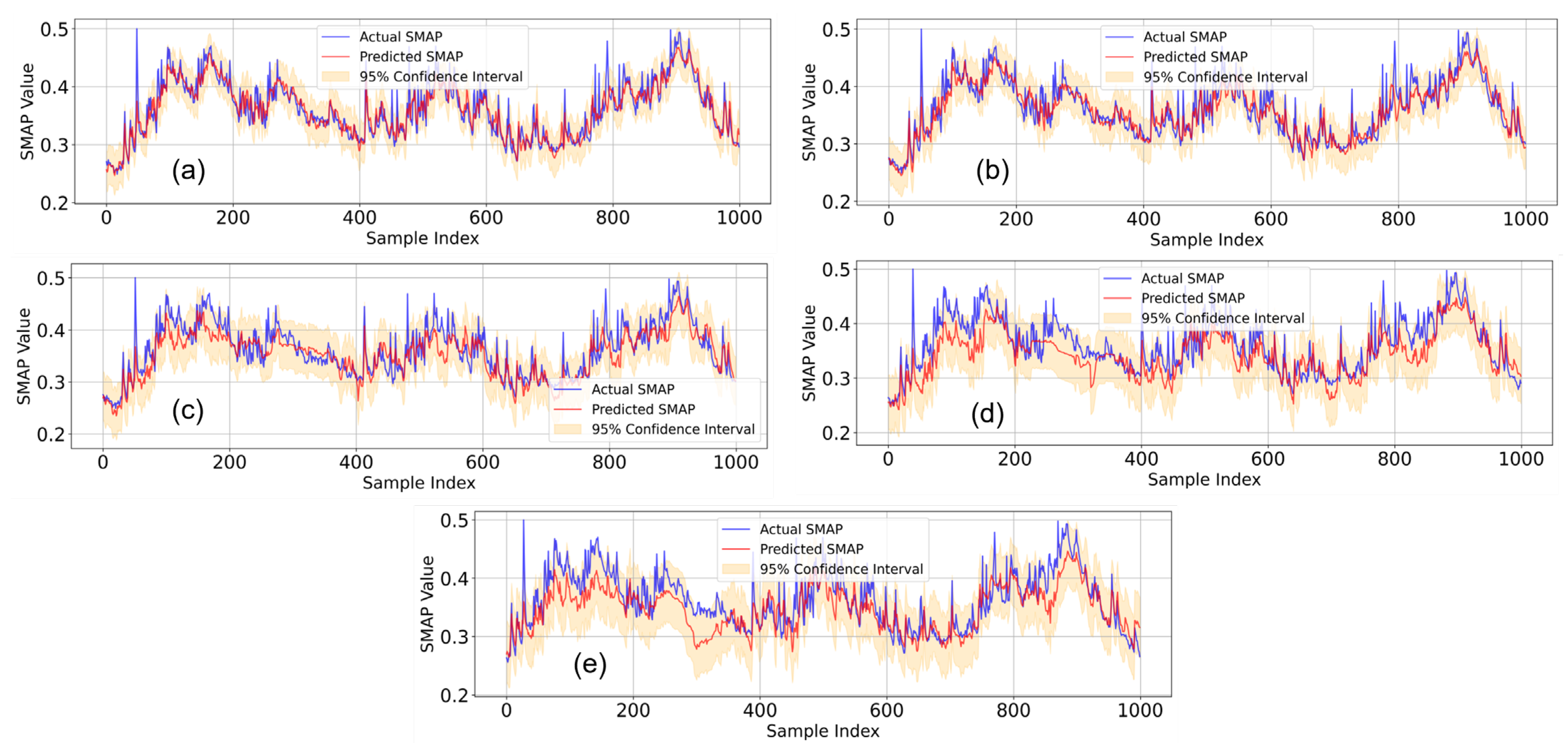
The standard deviation of residuals is an indicator of the dispersion of model prediction errors, reflecting the magnitude of fluctuations in the differences between actual and predicted values. As shown in Table 3, the residual standard deviation of our model ranges from 0.0169 to 0.0371, indicating relatively small and stable prediction errors. The 95% confidence interval of the model generally spans from 0.0332 to 0.0727, with a slight increase as the prediction step length increases. This implies that for any given prediction, we are 95% confident that the actual value will fall within the range defined by the confidence interval around the predicted value. The prediction range, calculated based on the standard deviation of residuals, provides the possible minimum and maximum values of the predictions. This range helps us understand the overall distribution of model predictions and identify any extreme or outlier values. The coverage probability (95% CI) indicates that the actual proportion of true values falling within the 95% confidence interval is greater than 94%, approaching or exceeding 95%. A high coverage probability suggests that the model’s uncertainty estimates are relatively accurate, meaning that the model can effectively capture the variations in actual values in most cases. Overall, the small residual standard deviation and narrow width of the 95% confidence interval indicate that the model has small and stable prediction errors, suggesting a good fit to the data and that high reliability of the prediction results. The prediction range (0.09–0.48) is consistent with the data range in practical applications, indicating that the model’s prediction range is reasonable.

Figure 7 presents a comparison between the actual SM values and the predicted values for the first 1000 validation samples, along with the uncertainty range of the 95% confidence interval predictions. The majority of the data points fall within the 95% confidence interval, indicating that the model’s predictions are well calibrated and reliable.

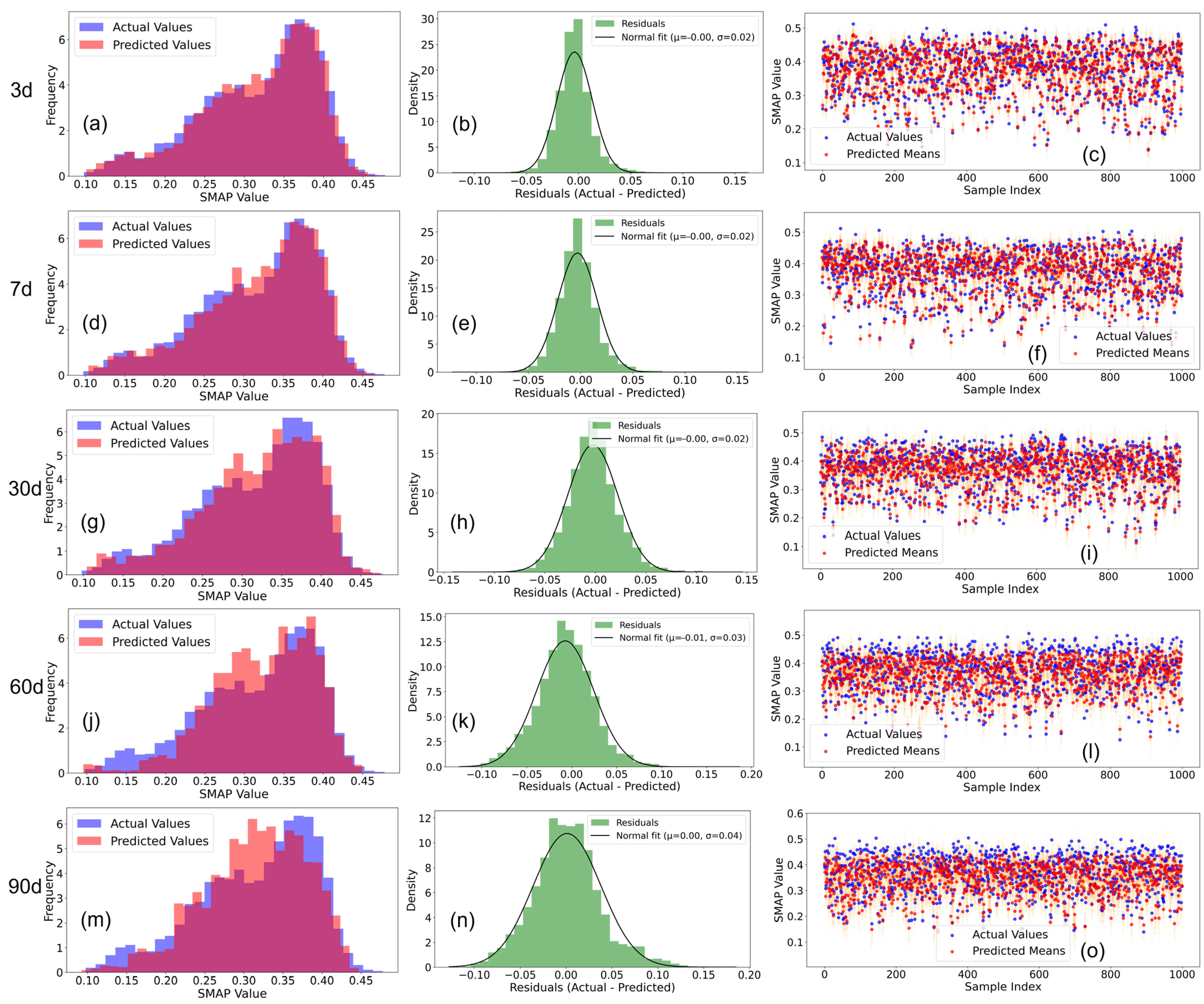
Figure 8 displays the distribution of predicted and actual SM using SMAP across different prediction steps. The overlap between the frequency distributions of predicted values and actual values is substantial, suggesting high prediction accuracy and minimal differences between predicted and actual values. The similarity in the tails of the distributions indicates that the model performs well in predicting extreme values. The ability of the predicted distribution to cover most of the actual distribution demonstrates that the model effectively captures the uncertainty in the data, with reasonable prediction intervals. The high coverage probability and narrow confidence intervals of the model indicate superior predictive performance and low uncertainty.

Residuals are listed in Table 2 for various prediction steps (3, 7, 30, 60, and 90 days). The distribution centers of the residuals range from 0.0169 to 0.0371, close to zero, indicating minimal deviation between predicted and actual values. The second column in Figure 8, showing the residual deviations, reveals that the residuals are approximately normally distributed, suggesting that the prediction errors are random and lack systematic bias. Although the standard deviation of the residuals increases slightly with longer prediction steps, the overall variability remains low, indicating stable model predictions. The bell-shaped distribution of residuals, close to a normal distribution, further confirms the random nature of prediction errors and the absence of systematic bias. The symmetry of the residual distribution indicates balanced prediction capabilities for positive and negative errors, while the short tails suggest few extreme errors, enhancing the reliability of the model’s predictions.

The third column in Figure 8 shows that the actual values and predicted values are closely aligned, indicating high prediction accuracy and minimal differences between predicted and actual values. The concentration of predicted values suggests stable model predictions with low variability. The model’s ability to predict extreme values, particularly within 30 days, demonstrates its robustness in handling anomalies.

3.6. Soil Moisture Simulation Distribution Maps

We conducted simulation predictions for SM on the 7, 30, 60, and 90 future days and compared the spatiotemporal distribution of SM predicted by the VIC-LSTMseq2seq model with the observations from the SMAP. As shown in Figure 9, the temporal and spatial variations in the observed values from SMAP and the simulation results for the 7, 30, 60, and 90 days are highly consistent. The predicted results closely match the observed results from SMAP in terms of both temporal trends and spatial patterns. In terms of temporal trends, the variations in SM across different prediction steps align well with the observed changes in 2022. In early August 2022, some regions experienced mild SM deficits, while other areas faced moderate deficits. As time progressed, the drought conditions continued to intensify, reaching their peak in October and November, when severe drought conditions were observed across almost the entire province. In mid-to-late November, rainfall alleviated the drought conditions, and the SM status improved significantly by December. Spatially, the distribution of mild, moderate, and severe SM deficits predicted by the model closely matches the observed patterns. These results that confirm the VIC-LSTMseq2seq model demonstrates strong simulation and predictive capabilities for SM on days 3, 7, 30, and 60 into the future, highlighting its exceptional forecasting performance.

4. Discussion

4.1. Soil Moisture Autocorrelation Analysis

To investigate the improvement effects of DL in SM simulation and prediction, we used the SMAP SM as the true value and conducted an analysis of the temporal autocorrelation characteristics of SM. In this study, we calculated the autocorrelation coefficients for individual sites and the entire dataset at different lag days (0–1000 days) to analyze the temporal memory effect of SM, as shown in Figure 10. The experimental results indicate that the data exhibit similar autocorrelation characteristics. Specifically, the most significant changes in the autocorrelation coefficients occur at lags below 10 days. At a lag of 2 days, the R is within 0.9, indicating extremely strong short-term correlation. Within 6 days, the R remains above 0.8, and it decreases as the lag time increases. Around a lag of 40 days, the autocorrelation of the sequence data drop to the level of 0.5, further reflecting the strong correlation between current drought conditions and previous droughts. Data from the past 40 days still have a certain predictive effect on current SM. Around a lag of 100 days, the autocorrelation of the sequence data drop to the level of 0–0.1. After a lag of 180 days, the data show fluctuating changes, which have distinct interannual variation characteristics. For short-term predictions (<10 days), relying solely on the autocorrelation of historical data can still yield relatively good simulation and prediction results. For medium-term predictions (10–40 days), the use of historical data still has some effect. However, for long-term predictions (>100 days), the effectiveness is less suitable. These findings provide a theoretical basis for the time-specific design of SM prediction models, confirming the important guiding role of temporal-scale characteristics in model architecture selection and feature engineering.

4.2. Comparison of Prediction Performance

By comparing the LSTM Seq2Seq model with traditional ML models such as the CNN and SVM, as well as with the LSTM model and advanced transformer model, it was found that the LSTM model outperformed other models in terms of prediction accuracy among the traditional models. In the field of SM prediction, although the LSTM model based on historical statistical methods can capture the autocorrelation characteristics of time series, its prediction accuracy decreases rapidly with the increase in the prediction step size. This is mainly because the LSTM model does not consider the “future” element and lacks constraints on future and physical processes, resulting in its prediction ability being limited by tis correlation with historical data and making it difficult to accurately represent the evolution characteristics of SM. For instance, Kratzert et al. [48] pointed out that the LSTM model performs well when dealing with nonlinear dynamic systems, but its performance is significantly limited when facing the prediction of long time series. To overcome this limitation, the coupled modeling method has gradually drawn attention. Some studies have combined the physical model with the LSTM model to construct a physical-guided ML model which performs better than the traditional historical data-driven LSTM model in hydrological simulation. Similarly, another study combined the meteorological forecast data from the European Centre for Medium-Range Weather Forecasts (ECMWFs) with the LSTM model to create a hybrid dynamic LSTM model, effectively predicting drought. This physical constraint mechanism enables the model to have a stronger error correction ability, thereby improving the stability of the prediction. Providing regularization constraints for the LSTM network using physical prior knowledge can significantly improve the error control ability of the model. Furthermore, through integrating physical laws and the advantages of ML, progress can be made in this field of research.

The LSTM Seq2Seq method is a novel method for SM prediction. Through the encoder–decoder architecture, it solves the problems of gradient disappearance and insufficient feature capture in traditional hybrid models when modeling long sequences. Compared with traditional LSTM or SVM and other classic ML models, Seq2Seq can better capture long-term dependencies, support multi-step predictions, and effectively integrate temporal and spatial features. This makes it perform better in SM prediction and means that it can more accurately reflect the trend of SM changes. The VIC-LSTMseq2seq model combines the physical mechanism with data learning by introducing the hydrological state simulation data generated by the VIC model, allowing for the ability to predict future scenarios. This coupling method not only retains the autocorrelation characteristics of the time series, but also introduces the predictive ability of the physical model for future scenarios. Models that introduce physical mechanisms can still maintain high simulation and prediction accuracy within a relatively long prediction step size. The innovation of the VIC-LSTMseq2seq model in this paper lies in its integration of the hydrological state simulation data generated by the VIC physical model, achieving a dual coupling of the physical mechanism and data learning. Meanwhile, this model takes into account the overall dependence of SM on historical meteorological and hydrological conditions. The features input into the model include historical features and simulated “future” hydrological state features. Moreover, the lengths and quantities of these features in the time series are different, facilitating efforts to solve the problem associated with the overall input of features of different lengths and allowing for the screening and selection of feature information related to soil to be avoided. The VIC-LSTMseq2seq model has achieved significant improvements in both prediction accuracy and physical rationality.

The coupled modeling method, combining physical models and DL techniques, can effectively improve the accuracy and stability of SM prediction. Future research can further explore how to optimize the interaction mechanism between physical models and DL models to achieve more efficient prediction performance.

4.3. Model Efficiency and Transferability

The LSTM Seq2Seq model structure in this study is relatively complex, and it requires a long training time due to its level of computational efficiency, requiring high-performance hardware support such as GPU acceleration. This experiment was executed on a computer with an Intel(R) Core(TM) i5-9400F CPU @ 2.90 GHz. One training process lasted for over half an hour. The model training costs were relatively high. However, by optimizing the architecture and parameters, the computational burden could be reduced to a certain extent. At the same time, this experiment included the features output by the VIC model, which also increased the complexity of the model. Due to the increase in running time and training costs, higher requirements were also imposed on the used hardware. Future research can further explore the adaptability of the model in different environments and optimize the computational efficiency.

The transferability of this research method is also worth discussing. Under different hydrological or climatic conditions, such as in arid or snow-covered areas, the differences in SM dynamics and processes such as precipitation and evaporation may affect model performance. For example, SM in arid areas is more sensitive to precipitation, while in snow-covered areas, the melting of snow needs to be considered with regards to the replenishment of moisture. In addition, the availability of the VIC model and SMAP data is limited, posing certain limitations to this research, and missing data or insufficient accuracy of the model may affect the model’s training and prediction results.

4.4. Impact of the Datasets Used

To analyze the effectiveness of the proposed model in simulating daily-scale SM and to construct a SM prediction model with high accuracy and applicability for daily operational use, this study utilized the SMAP L4 SM. Although SMAP L4 data have an acquisition delay of 2–3 days, the correlation coefficient for simulating and predicting SM up to 7 days in the future still exceeds 0.96. Therefore, it can be considered the primary data source for SM simulation, offering high spatiotemporal continuity and accuracy. Despite the advantages of its temporal resolution its complete spatial coverage of SMAP data, the process of downscaling it to a 0.0625° resolution may have introduced scale errors. To improve data quality, future work could involve integrating multi-source satellite data (e.g., Sentinel-1) for joint calibration and for developing dynamic bias correction algorithms that account for soil texture and vegetation cover. Additionally, optimizing the layout of ground-based observation stations can enhance the spatial representativeness and temporal continuity of in situ data. In terms of feature engineering, this study innovatively combined 30 days of historical meteorological observations (seven features, including precipitation, wind speed, and temperature) with hydrological elements simulated by the VIC model for the next M days (six features, including evaporation and runoff). Although this combination of features at different temporal scales can characterize SM dynamics, errors in meteorological observations and uncertainties in VIC model parameterization may propagate through the features and affect prediction results. Future work could introduce data assimilation techniques to reduce initial condition errors and employ ensemble forecasting methods to quantify model uncertainty, thereby further enhancing the robustness of the prediction system.

4.5. Future Directions for Improving Explainability of Deep Learning Models

This study innovatively constructed a DL model based on a fusion of multi-source data, proposing a multimodal fusion architecture that integrates past meteorological observations with future hydrological simulations. It effectively addressed the issue of insufficient feature utilization in traditional methods, developed a heterogeneous feature encoding mechanism for SM prediction, and established a joint calibration framework between SMAP satellite data and ground observations. These advancements significantly improved the quality and reliability of the input data, enabling the high-precision temporal prediction of SM. This not only provides a new technical means for regional SM monitoring but also offers a paradigm for multi-source data fusion modeling in the field of hydro-meteorology.

In terms of model explainability, future research will focus on three important trends: first, the development of physics-informed explainable AI (XAI) techniques, which embed hydrological process equations as differential constraints within neural networks to achieve bidirectional validation between prediction results and physical mechanisms; second, the innovation value of dynamic explainability methods, which develop time-aware feature importance analysis tools to reveal the temporal variations in SM memory effects; third, the refinement of multimodal explanation frameworks, which establish a unified evaluation system capable of parsing the contributions of multi-source data, including remote sensing observations, ground monitoring data, and model simulations. Developing this field on research in these directions will further enhance the credibility and application value of DL models in the field of hydrology, providing more reliable decision support for smart agriculture and water resource management.

5. Conclusions

This study introduced an SM simulation model, VIC-LSTMseq2seq, which couples the VIC land surface hydrological model with DL. The model considers both past SM states and historical time series dependencies, as well as future states simulated by the VIC model. By integrating an encoder–decoder architecture with feature attention mechanisms (AMs) and LSTM networks, the model can handle inputs with varying temporal steps and feature counts. Comprehensive evaluations demonstrate that the VIC-LSTMseq2seq model outperforms traditional statistical LSTM models in SM simulation and prediction tasks, particularly in terms of accuracy and reliability. It shows great potential for drought simulation and prediction.

It should be noted that although the VIC-LSTMseq2seq model achieved satisfactory prediction results in this study, its performance may be influenced by regional geographical characteristics, soil type differences, and climate change factors. The model’s generalizability across different regions needs to be validated through the use of a broader range of geographical samples. Additionally, the current study mainly focused on improving prediction performance, with relatively limited research on the explainability of the model’s internal mechanisms being conducted.

Future research can follow the following three recommendations in depth. Firstly, researchers should conduct multi-scale validation experiments to systematically assess this model’s applicability in different climatic zones and soil types. Secondly, they should develop hybrid modeling methods that incorporate physical mechanisms by embedding hydrological process equations as constraints within neural networks to enhance the model’s physical explainability. Finally, they should explore strategies for implementing the model in practical applications such as smart agriculture and water resource management, particularly focusing on how to effectively integrate model predictions into existing decision support systems. These studies will not only help further refine the VIC-LSTMseq2seq model but also provide new ideas for the development of intelligent prediction methods in the field of hydro-meteorology.