Article

Precipitation Governs Terrestrial Water Storage Anomaly Decline in the Hengduan Mountains Region, China, Amid Climate Change

1
School of Geographical Sciences, China West Normal University, Nanchong 637009, China
2
Sichuan Provincial Engineering Research Center of Monitoring and Control for Soil Erosion in Dry Valleys, China West Normal University, Nanchong 637009, China
3
College of Geography and Remote Sensing Science, Xinjiang University, Urumqi 830046, China
4
Xinjiang Key Laboratory of Oasis Ecology, Xinjiang University, Urumqi 830046, China
*
Author to whom correspondence should be addressed.
Remote Sens. 2025, 17(14), 2447; https://doi.org/10.3390/rs17142447
Submission received: 12 June 2025 / Revised: 6 July 2025 / Accepted: 11 July 2025 / Published: 15 July 2025

Abstract

Climate change intensifies hydrological cycles, leading to an increased variability in terrestrial water storage anomalies (TWSAs) and a heightened drought risk. Understanding the spatiotemporal dynamics of TWSAs and their driving factors is crucial for sustainable water management. While previous studies have primarily attributed TWSAs to regional factors, this study employs wavelet coherence, partial correlation analysis, and multiple linear regression to comprehensively analyze TWSA dynamics and their drivers in the Hengduan Mountains (HDM) region from 2003 to 2022, incorporating both regional and global influences. Additionally, dry–wet variations were quantified using the GRACE-based Drought Severity Index (GRACE-DSI). Key findings include the following: The annual mean TWSA showed a non-significant decreasing trend (−2.83 mm/y, p > 0.05), accompanied by increased interannual variability. Notably, approximately 36.22% of the pixels in the western HDM region exhibited a significantly decreasing trend. The Nujiang River Basin (NRB) (−17.17 mm/y, p < 0.01) and the Lancang (−17.17 mm/y, p < 0.01) River Basin experienced the most pronounced declines. Regional factors—particularly precipitation (PRE)—drove TWSA in 59% of the HDM region, followed by potential evapotranspiration (PET, 28%) and vegetation dynamics (13%). Among global factors, the North Atlantic Oscillation showed a weak correlation with TWSAs (r = −0.19), indirectly affecting it via winter PET (r = −0.56, p < 0.05). The decline in TWSAs corresponds to an elevated drought risk, notably in the NRB, which recorded the largest GRACE-DSI decline (slope = −0.011, p < 0.05). This study links TWSAs to climate drivers and drought risk, offering a framework for improving water resource management and drought preparedness in climate-sensitive mountain regions.

1. Introduction

Global warming has accelerated the water cycle in recent decades, exacerbating the global water scarcity crisis. Approximately 80% of the world’s population faces water insecurity or severe water scarcity, driven by climate variability and human activities, which is deepening under ongoing climate change [1,2]. Terrestrial water storage (TWS), mainly composed of surface waters (rivers, lakes, reservoirs, swamps, and wetlands), soil moisture, ice, snow water equivalent and groundwater, serves as a critical indicator of water resource availability and climate change, playing a pivotal role in irrigation, domestic water supply, and industrial production [3,4,5]. TWS anomalies (TWSAs) serve as a critical indicator for monitoring climate change and water-related disasters, such as floods and droughts, owing to their strong correlation with various components of the water budget [6,7]. However, TWSAs exhibit complex spatiotemporal variability with nonlinear and lagged impacts on ecosystem processes and water resource management [5,8]. Therefore, accurately quantifying long-term TWSAs and exploring their attribution response to climate change will benefit scientific decision-making and sustainable water resource management.
TWSA acquisition has traditionally relied on land surface or global hydrological models that calculate the sum of all related TWSA components, or the water balance method that measures all related hydrological fluxes, including precipitation, evaporation, and river discharge [5,9,10,11]. However, due to the high spatiotemporal variations in TWSAs and the lack of long-term and intensive in situ observations, it is difficult to accurately estimate long-term TWSAs at large spatial scales [12,13]. Since its launch in 2002 by the National Aeronautics and Space Administration (NASA) and the German Aerospace Centre, the Gravity Recovery and Climate Experiment (GRACE) satellites have revolutionized TWSA evaluation, providing an effective tool for assessing hydrological changes [1,14]. GRACE data have been widely used to evaluate the groundwater potential, storage capacity, drought, and river runoff [11,15]. Despite its advantages, GRACE-derived products are constrained by their coarse spatial resolution (the effective resolution is approximately 300–500 km in terms of a half-wavelength (which is equivalent to a surface area of ~90,000–250,000 km2)) and an 11-month data gap (July 2017 to May 2018), limiting their application in regional studies [14]. To address these limitations, researchers have increasingly turned to machine learning techniques (ML) and statistical models to reconstruct TWSAs by establishing empirical relationships between GRACE TWSAs and climatic, hydrological, and underlying surface parameters [11,16,17,18]. For example, Zhang et al. (2024) [19] developed a TWSA dataset with a spatial resolution of 0.1° using a Bayesian approach, demonstrating high and continuous spatial accuracy.
TWSAs arise from the intricate interactions between climate variability and human activities [13,20]. They are shaped by the dynamic interplay of fluctuating water supply and demand, and exhibit significant complexity across different regional and global scales, with varying dominant factors in different latitudes [5,8,13]. At the regional level, factors such as climate, topography, land cover, and human activities significantly shape the TWSA dynamics [8,21,22]. However, the exact causes of observed TWSAs remain elusive, with regional factors such as human-induced water withdrawals, atmospheric demand (potential evapotranspiration, PET), PRE variability, and vegetation greening (increasing the normalized difference vegetation index (NDVI)) contributing to the complexity [20,23,24]. While PRE is often identified as the primary factor [21], vegetation greening has also been highlighted as a significant driver. Chen et al. (2024) [25] reported that vegetation restoration is more significant than climate factors in the TWSA decline hotspots within the Three-North region of China. Meanwhile, Meng et al. (2019) [26] indicated that TWSAs in the entire Tibetan Plateau from 2003 to 2014 are attributed largely to variations in PRE and evapotranspiration (ET). TWSA studies in China have focused on regions sensitive to climate change and vegetation restoration, such as, the Three-North region [25], the Yangtze River Catchment [27], the Taihang Mountain Region [4], the Karst Plateau in Southwest China [15], Mu Us Sandyland [28], and the Tibetan Plateau [29]. These studies have explored the spatiotemporal patterns and drivers of TWSAs, including groundwater depletion, glacier loss, drought and flood dynamics, and ecosystem responses [20,25,30,31,32]. However, spatial heterogeneity in dominant drivers further complicates the understanding of TWSA dynamics.
Global, atmospheric oscillations, including the North Atlantic Oscillation (NAO), Pacific Decadal Oscillation (PDO), Arctic Oscillation (AO), and El Niño-Southern Oscillation (ENSO), also play a pivotal role in driving TWS [9,33,34]. Recent studies [7,35] have explored the relationship between TWSAs and climate teleconnection factors on both global and continental scales. For instance, several studies have shown a strong correlation between the interannual variations in TWSAs between 15°S and 15°N [16,34]. Scanlon et al. (2023) [35] demonstrated that the interannual TWSA variability in eastern and southern Africa is predominantly influenced by extreme climate events, with teleconnections, such as ENSO and the Indian Ocean Dipole (IOD), playing a significant role in drought and flood occurrences. While extensive research has been conducted on the impacts of large-scale atmospheric circulations on climatic factors, such as PRE, runoff, PET, and drought conditions [36,37,38], studies focusing specifically on the direct effects of global teleconnection factors on TWSAs remain limited. Additionally, the combined effects of multiple factors across multiple timescales have not been fully explored [39].
TWSAs drive significant spatiotemporal shifts in surface dry–wet conditions, thereby amplifying the risks of hydrological extremes, including droughts and floods [40]. GRACE-derived drought indices have proven to be effective tools for quantifying these hydrological imbalances. Thomas et al. (2017) [41] demonstrated that GRACE-based indices reliably capture the onset, duration, and severity of droughts, showing strong alignment with established meteorological drought databases. In China’s exorheic basins, GRACE-based indices exhibit robust agreement with the drought indices derived from meteorological datasets [40]. This underscores the utility of TWSAs in quantifying water deficits and analyzing the dry–wet characteristics in specific regions, providing a valuable framework for further exploring their broader impacts on hydrological systems.
The Hengduan Mountains (HDM) region, located in the southeastern Tibetan Plateau, is characterized by a series of high, north–south oriented mountain ranges. It is recognized as one of the world’s most ecologically sensitive regions, distinguished by its complex topography, diverse ecosystems, and unique climatic influences [42,43,44]. As the source of major branches of the upper Yangtze and Pearl Rivers, as well as several transboundary rivers (e.g., the Mekong and Salween), the HDM region plays a critical role in regional and downstream water security [42,44]. Furthermore, the region’s topography creates a ‘foehn’ effect, resulting in the formation of the well-known ‘arid valley’ and thereby intensifying the threat of drought. In recent decades, the HDM region has experienced increasing water stress due to the combined effects of climate change and human activities. For instance, the region suffered severe “autumn–winter–spring” droughts from 2009 to 2012, during which the river flows declined by 30–80% of their normal volumes, with some rivers completely drying up [45]. These highlight the region’s vulnerability to climatic variability and the urgent need for effective water resource management. However, hydrological complexity induces pronounced spatiotemporal variability in TWSAs across the HDM region. Few studies have comprehensively quantified the combined impacts of multiple drivers on TWSAs. Therefore, it is imperative to understand the spatiotemporal patterns of TWSAs and, particularly, their impacting factors in the HDM region.
Despite the above-mentioned studies, the complex interplay of regional and global factors influencing TWSAs is yet to be quantitatively characterized. This can be achieved by following a framework of “patterns-drivers-impacts”. The primary objectives of this study are as follows: (1) To determine the spatiotemporal characteristics of TWSAs in the HDM from 2003 to 2022. (2) To correlate the TWSA changes with regional and global climate variables. (3) To understand the relationship between TWSAs and dry–wet characteristics. This study provides valuable insights for sustainable water resource management in high-altitude mountainous areas with complex terrain worldwide. These findings will support the development of more effective and targeted water resource management strategies, providing a crucial foundation for mitigating drought risks and enhancing regional water security in these vulnerable environments.

2. Materials and Methods

2.1. Study Area

The HDM region is situated in southwest China, bordering the Qinghai–Tibet Plateau in the west and connecting the Sichuan Basin and the Yunnan–Guizhou Plateau in the east. It serves as a transitional zone between China’s first and second topographic terraces. Its lowest point is at 326 m while its highest peak is at 6580 m. The region includes the upper reaches of several major rivers in China and Southeast Asia and features a well-developed drainage network, with high mountains and deep valleys shaped by numerous north–south flowing rivers. The HDM region is influenced by the high-altitude westerly circulation, as well as the Indian Ocean and Pacific Ocean monsoons. Its PRE patterns differ significantly from those of other regions of the country that lie at the same latitude. The distinction between wet and dry seasons is pronounced: the wet season typically lasts from mid-May to mid-October, accounting for ≥85% of the annual PRE, while the dry season spans from mid-October to mid-May of the following year, characterized by minimal rainfall, prolonged sunshine, high evaporation rates, and dry air [43]. The vegetation cover is dominated by forest and grassland (Figure 1e). The complex natural environment and abundant plant resources make it one of the world’s most biodiverse areas and a priority for ecological conservation [44].
The river and basin boundaries in this study were delineated based on hydrological divisions, spanning from west to east as follows (Figure 1b): the Nujiang River Basin (NRB) (Upper Salween River catchment within China’s territory), the Lancang River Basin (LRB) (Headwaters of the Mekong River), the Yalong River Basin (YRB), and the Minjiang River Basin (MRB) (Data source: Resource and Environment Science and Data Center).

2.2. Methodology and Data Sources

2.2.1. Datasets

TWSA data were obtained from the GRACE mission and its successor, GRACE Follow-On (GRACE-FO). The GRACE mission was launched in March 2002 and concluded in June 2017. GRACE-FO was launched in May 2018 and is providing continuous observations. GRACE monitors temporal variations in Earth’s gravity field, which are used to infer changes in TWSAs, expressed as equivalent water thickness [46]. A GRACE-derived TWSA represents the integrated changes in all forms of water storage anomalies, including surface and subsurface components [21,32], and can be expressed as:
T W S A = G W S + S W S + S W E + C W S + S M S
where G W S , S W S , S M S , S W E , and C W S   denote the anomalies in groundwater storage, surface water storage, soil moisture storage, snow water equivalent, and canopy water storage, respectively.
The monthly TWSA data used in this study were generated by Zhang et al. (2024) [19] using a Bayesian-based triple collocation method, which fused GRACE-derived TWSA/GWSA products with low uncertainty at a coarse resolution of 0.5°. They developed a physically constrained sliding-window ML downscaling framework to integrate the fused TWSA/GWSA products with multi-source datasets, producing a high-resolution (0.05°), gap-free global product known as High-Resolution Water Storage Anomalies (HWSA v1.0) (data available at https://data.tpdc.ac.cn/en/data/42176bad-0d38-4a84-9f87-3c2c06eb19b8, accessed on 10 November 2024) [19]. This study focuses on TWSA data spanning from January 2003 to December 2022.
Recently, the Goddard Space Flight Center (GSFC; https://earth.gsfc.nasa.gov/geo/data/grace-mascons, accessed on 12 December 2024), the Center for Space Research (CSR; https://www2.csr.utexas.edu/grace, accessed on 12 December 2024), and the Jet Propulsion Laboratory (JPL; https://grace.jpl.nasa.gov, accessed on 12 December 2024) have released a new generation of GRACE/GRACE-FO observation products, known as Mascon products [47], which incorporate regularization techniques in data processing, enabling direct computation of TWSAs from Level 1B data [48]. This study employed GRACE Level 3 products based on spherical harmonic solutions (Release 5, RL05). These data are primarily used for comparative evaluations of the accuracy of HWSA results.
We attributed TWSAs to various factors, including meteorological and vegetation variables, as well as global teleconnection indices. Specifically, we considered two meteorological variables—the monthly PRE and the PET—and one vegetation variable (the NDVI) [8]. Climate factors were obtained from the TerraClimate dataset (available at: https://climate.northwestknowledge.net/TERRACLIMATE/, accessed on 12 December 2024), which employs a climate-aided interpolation method, combining the high spatial resolution of the WorldClim dataset with the temporal variability of CRU Ts4.0 and the Japanese 55-year Reanalysis (JRA-55, 1958–2012) [49]. The final dataset has a spatial resolution of 0.1° × 0.1°. Further details on these datasets are provided in Table 1.
The NDVI, a key vegetation indicator, is calculated as the normalized ratio of near-infrared radiation to red reflectance, providing a quantitative measure of vegetation greenness. NDVI data were obtained from the Aqua/Terra-Moderate Resolution Imaging Spectroradiometer satellite sensor (MOD13Q1), with an original spatial resolution of 250 m. The data processing workflow included a reconstruction of similar feature noise pixels, application of a Savitzky–Golay filter to long-term series images, quality control, and monthly compositing and mosaicking [50]. The dataset is available at https://data.tpdc.ac.cn/zh-hans/data/10535b0b-8502-4465-bc53-78bcf24387b3, accessed on 12 December 2024. To align with the spatial resolution of GRACE-derived TWSAs, all data were resampled using a bilinear interpolation method to a resolution of 0.05° × 0.05°.
To account for the influence of large-scale atmospheric circulation, four key global climate indices were selected: the NAO, AO, PDO, and ENSO [51,52]. The NAO, defined by the pressure difference between the Icelandic Low and Azores High, strongly influences winter temperatures in northern China, with stronger NAOs linked to milder winters [53]. The AO, the dominant mode of winter sea-level pressure variability, affects westerly winds and the East Asian winter monsoon, shaping China’s winter climate. Monthly AO and NAO indices were sourced from NOAA (https://www.cpc.ncep.noaa.gov/products/precip/CWlink/daily_ao_index/ao.shtml, accessed on 12 November 2024). The PDO, derived from North Pacific Sea surface temperature anomalies, indicates decadal climate variability [54]. The ENSO, measured by the Niño 3.4 index (equatorial Pacific SST anomalies), drives tropical PRE and global climate patterns. Niño 3.4 and PDO data were obtained from the National Center for Atmospheric Research (https://climatedataguide.ucar.edu/climate-data, accessed on 12 November 2024). The seasons are categorized as follows: spring (March–May), summer (June–August), autumn (September–November), and winter (December–February).
Table 1. Overview of datasets employed in this research.
CategoriesIndices and AggregationNameResolutionSources
Water storageTerrestrial water storage (TWSA)HWSAMonthly, 0.05°, covered period: 2002.04–2022.12[19]
CSRMonthly; 1°
covered period: 2002.04–2022.12
[48]
JPLMonthly; 0.5° covered period: 2002.04–2022.12[55]
GSFCMonthly; 0.5° covered period: 2002.04–2022.12[47]
VegetationNormalized difference vegetation index (NDVI)Monthly, 250 mMOD13Q1
[50]
ClimatePrecipitation (PRE)Monthly, 0.1°TerraClimate
[49]
Potential Evapotranspiration (PET)

2.2.2. Theil–Sen Median Trend Analysis and Mann–Kendall (M–K) Test Statistics

To analyze the long-term trends in TWSAs and their driving factors in the HDM region, the Theil–Sen median trend and MK trend test method [56,57] were employed. The MK method is commonly employed to evaluate the significance of trends in hydro-meteorological time series [58,59]. Sen’s slope can be expressed by the following equation:
β = M e d i a n x i x j i j , j < i
where β presents a robust estimate of the trend magnitude, while xi and xj donate the ith and jth observations, respectively (where ij < ≤ n). A positive value of β signifies an increasing trend and vice versa.
The test statistic K is calculated as follows:
S = i = 1 n 1 · j = i + 1 n s g n ( x j x i )
where xj and xi are the data results at times j and i (j > i), sgn (xjxi) is the sign function, and n is the number of data points. The sign function is defined as:
s g n x j x i = 0 ,   + 1 ,     i f x j x i > 0                 i f x j x i = 0 1 ,           i f   x j x i < 0
For sample sizes n > 10, the variance V is calculated as:
V = n n 1 2 n + 5 k = 1 p t k ( t k 1 ) ( 2 t k + 5 ) 18
where tk is the number of ties in the kth group, and p is the number of ties. The test statistic S is approximately normally distributed and can be transformed into a standard normal distribution using the Z-score:
Z = 0 ,   S 1 V ( S ) ,     i f   S > 0                 i f   S = 0 S + 1 V ( S ) ,           i f   S < 0
Positive and negative values of Z indicate increasing and decreasing trends, respectively. A 5% significance level was used, and the null hypothesis of no trend was rejected if |Zs| > 1.96.

2.2.3. Partial Correlation Coefficient

To better understand the correlation of TWSAs and climatic variables, partial correlation analysis was conducted, which measures the degree of association between two variables while controlling the influence of other variables. For example, the formula for the first-order partial correlation coefficient is as follows:
r 123 = r 12 r 13 r 23 1 r 13 2 1 r 23 2
where r 123 is the partial correlation coefficient between factors 1 and 2 after removing the effect of variable 3. Similarly, r 12 ,   r 13 and r 23 are the pairwise correlation coefficients between the respective variables.

2.2.4. Attribution Analysis

To identify the dominant factors driving the spatiotemporal variations in monthly TWSAs at the grid-cell level, a multiple linear regression (MLR) model was applied. This approach quantifies both the relative influence (normalized contribution) and absolute contribution (magnitude of effect) of individual explanatory variables on TWSA dynamics. The model is expressed as follows:
T W S A = β 0 + β 1 X 1 + β 2 X 2 + + β n X n + ε
where β 0 is the intercept variable, β 1 ,   β 2 ,   , β n are the regression coefficients corresponding to the explanatory variables, X 1 ,   X 2 , , X n   and ε is the residual error, and n denotes the number of independent variables. Model performance was assessed using the coefficient of determination (R2) and significance testing (p < 0.05).
Each dataset was normalized to ensure comparability across variables with different units:
X m = x m i n ( x ) max x m i n ( x )
where Xm is the normalized data of TWSAs and their driving factors, including PET, PRE, and the NDVI.
The relative and absolute contributions of each factor to a TWSA were quantified using the regression coefficients and standardized trends of the respective driving factors:
η c 1 = a 1 × X 1 s _ t r e n d
where η c 1 is the contribution of a driving factor to TWSAs.
Relative contribution measures the proportion of the total variability in TWSAs explained by a specific factor:
η r c 1 = η c 1 i = 1 n η c i
The actual contribution quantifies the magnitude of the effect of a specific factor on TWSAs:
η a c = η c 1 Y n _ t r e n d × Y t r e n d
where η r c 1 and η a c   are the relative contribution of driving factors, and the absolute contribution amounts, respectively.

2.2.5. Wavelet Coherence Analysis (WCA)

WCA was employed to investigate the temporal correlations between TWSAs and the ENSO, PDO, NAO, and AO over the period 2003–2022. WCA is a coherence analysis technique based on wavelet analysis, which provides insights into the coherence of signals across different scales [60].
The wavelet coherence R n 2 s is defined as:
R n 2 s = S s 1 W n X Y s 2 S s 1 W n X ( s ) 2 × s 1 W n Y ( s ) 2
where s is the scale, S is the smoothing operator, W n X ( s ) and W n Y ( s ) are the wavelet coefficients of the X and Y series, respectively, and W n X Y s is the reciprocal spectrum of the X and Y series. The analysis was performed using the “WaveletComp” and “biwavelet” packages in R version 4.4.2.

2.2.6. GRACE-Drought Severity Index (GRACE-DSI)

The GRACE-DSI was used to assess dry–wet characteristics based on TWS variations. It enables the comparison of drought severity across regions and time intervals without being influenced by uncertainties associated with soil moisture balance models or meteorological data [61]. The GRACE-DSI (dimensionless) is calculated as:
G R A C E D S I i , j = T W S i , j T W S j ¯ σ j
where i and j are the year (ranging from 2003 to 2022) and month (January–December), respectively; T W S j ¯ and σ j are the mean and standard deviation of month anomalies, respectively. Following Zhao et al. (2017) [61], its values can be classified into different drought severity categories (Table 2).

3. Results

3.1. Evaluation of TWSA Dataset Accuracy in the HDM Region

To evaluate the accuracy of the HWSA product, we compared its temporal trend of monthly values with multi-source TWSA products (CSR, JPL, and GSFC) (Figure 2). The correlation coefficients between HWSA and the three mascon products were high (0.94–0.98, p < 0.001) in the HDM region during 2003–2022. Notably, the correlation coefficient between HWSA and JPL reached 0.98, and the RMSE ranged from 1.30 to 2.69 cm/month. The high correlation and low RMSE observed between HWSA and JPL indicate strong agreement between the HWSA product and GRACE mascon TWSA products.
In summary, the results show that the differences are relatively small, suggesting that the HWSA product effectively captures TWSA trends across the HDM region and demonstrates utility for subsequent quantitative assessments of hydrological dynamics.

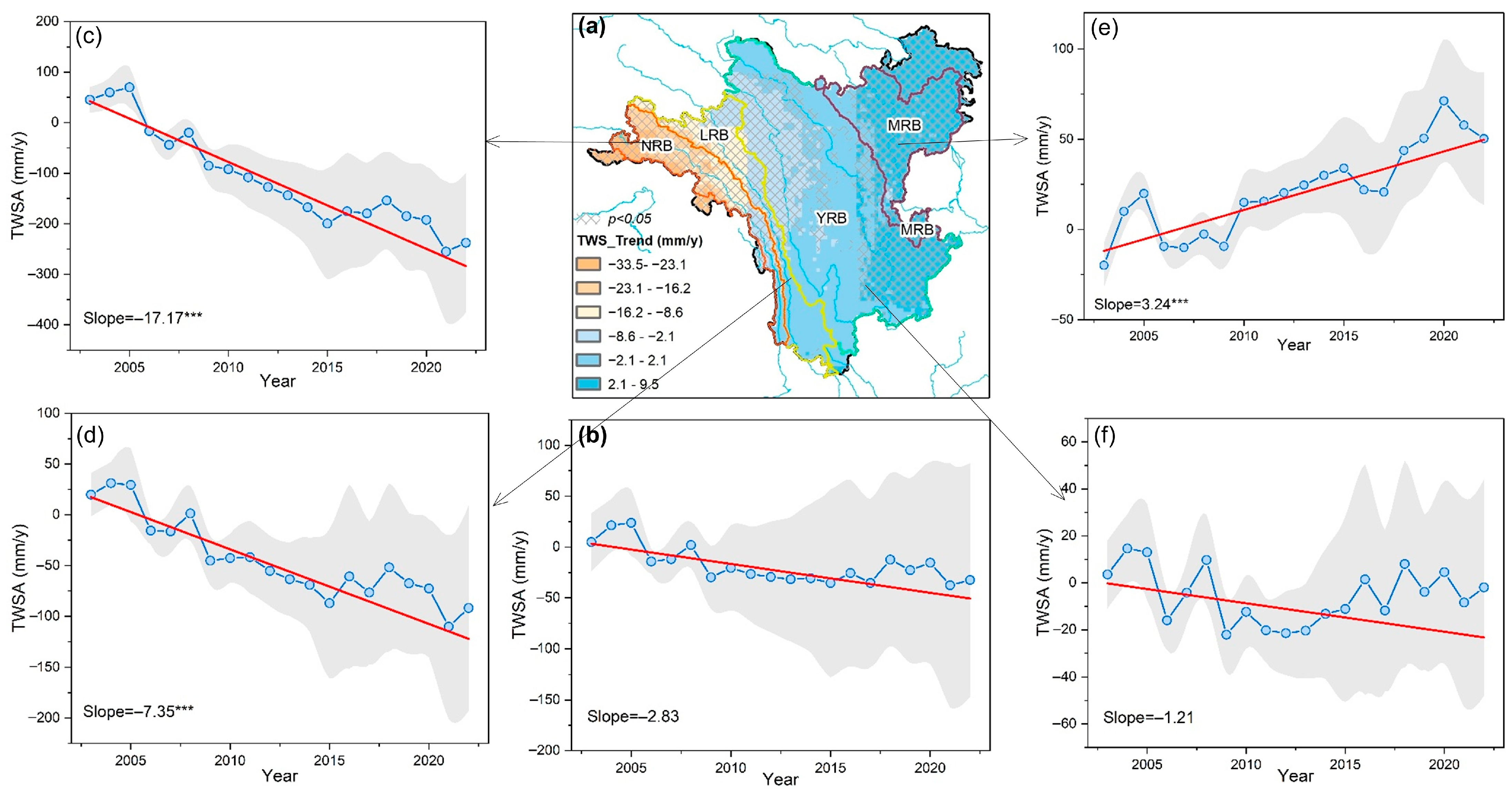
3.2. Spatiotemporal Changes in TWSA in the HDM Region

To explore the spatiotemporal characteristics of the TWSA, the seasonal and annual average variations are presented in Figure 3 and Figure 4. The linear trends of TWSAs across the HDM region were analyzed for each watershed from 2003 to 2022 (Figure 3). Significant negative trends (p < 0.05, M–K test) were observed in the eastern and western parts of the HDM region. From 2003 to 2007, ~33.85% of the TWSAs exhibited a significantly increasing trend, primarily concentrated in the eastern HDM region, including the MRB and parts of the TRB. In contrast, ~36.22% of the TWSAs showed a significant decreasing trend, mainly in the western portion of the study area, particularly in the NRB and parts of the LRB. Additionally, 17.36% and 12.57% of the area displayed non-significant increasing and decreasing trends, respectively.
In terms of interannual variation, the TWSAs in the HDM region exhibited a non-significant decreasing trend of −2.83 mm/y (p > 0.05). The average annual TWSAs declined to a range of approximately −12.39 to −32.44 mm/y. The TWSAs showed a significant downward shift, indicating a substantial reduction in TWSAs within the HDM region. Notably, the standard deviation of TWSAs has increased each year, suggesting more pronounced fluctuations in TWSAs, likely driven by multiple influencing factors.
Among the river basins, the NRB experienced the most significant decline in TWSAs, with a trend of −17.17 mm/y (p < 0.05), followed by the LRB with a trend of −7.35 mm/y. In contrast, the MRB exhibited a significant increasing trend in TWSAs, with a rate of 3.24 mm/y (p < 0.001), while the YRB showed a non-significant decreasing trend (slope =−1.21 mm/y, p > 0.05). These findings highlight that the spatial variations in TWSAs are governed by diverse factors.
To further elucidate the multi-scale temporal characteristics of TWSAs, we analyzed their monthly and seasonal variations from 2003 to 2022. The results (Figure 4) reveal that TWSAs exhibited an increasing trend from March to September and a decreasing trend during the remaining months. Monthly TWSAs fluctuated between −110.69 and 97.47 mm, with the maximum value observed in September 2004 and the minimum value recorded in April 2021. On average, August showed the largest value of TWSAs at 40.68 mm/month, whereas March exhibited the strongest decrease at −66.41 mm/month. On a seasonal scale, the multi-year mean indicated an increasing trend in summer and autumn. The fastest rate of decline occurred in spring (−2.52 mm, p < 0.01), followed by summer (−2.28 mm, p < 0.01). Although TWSAs declined the most in winter, the trend was relatively small (−1.51 mm, p < 0.01).
The spatial distribution of the average and trend of TWSAs in the HDM region was analyzed for each season (Figure 5). In spring (Figure 5a), TWSAs exhibited a significant decreasing trend (up to −20 mm/y, p < 0.01) in the western portion of the study area, contrasting with an increasing trend in the eastern region. This spatial pattern suggests a distinct east-west gradient in TWSA dynamics during spring. During summer (Figure 5b), the spatial distribution of TWSAs resembled that of spring, but the area characterized by increasing TWSAs expanded further. In autumn (Figure 5c) and winter (Figure 5d), the spatial patterns of TWSAs were generally similar to those observed in spring and summer. However, the trends in some regions did not reach statistical significance, indicating a potential weakening of the driving factors or increased variability in TWSAs during these seasons. This seasonal variability highlights the complex interplay of climatic, hydrological, and anthropogenic factors influencing TWSA dynamics in the region.

3.3. Spatiotemporal Variability of Driving Factors

The availability and demand for atmospheric moisture serve as key climatic factors affecting TWSAs [20]. Their impacts are further modulated by vegetation variations [25]. Figure 6 and Figure S2 show the spatial patterns of the three environmental factors (PRE, PET, and NDVI) in the HDM region. PRE displayed a significant increasing trend in 3.19% of the total grid cells across the HDM region; these significant increases were primarily concentrated in the southeastern part of the HDM region, where the trend exceeded 6.6 mm/y. Among all identified increases, 59.65% were not statistically significant increases (p > 0.05), and these mainly occurred in the northern part of the study area. Conversely, decreasing but insignificant trends in PRE were mainly observed in the southwestern part of the HDM region. For PET, most grid cells showed an increasing trend, though these trends did not pass the significance test. Only 5.36% of the grid cells exhibited a statistically significant increasing trend, primarily located in the northern part of the HDM. Additionally, PET showed no significant increase in 49.50% of the study area, while a small fraction (1.22%) exhibited a significant decreasing trend. The NDVI displayed an increasing trend in 26.26% of the grid cells within the southeastern part of the HDM, with 53.94% of these trends being statistically non-significant and concentrated in the eastern part. In contrast, NDVI showed a significant decreasing trend in 2.46% of the region.
Temporally, the PRE, PET, and NDVI all exhibited increasing trends across the entire HDM region (Figure S1). At the sub-basin level, the MRB showed a significant increase in PRE with an interannual trend of 3 mm/y, while the YRB exhibited a non-significant trend. In contrast, the LRB and NRB showed non-significant decreasing trends in PRE. For PET, the NRB displayed a significantly increasing trend of 1 mm/y, followed by the MRB with a trend of 0.4 mm/y. In contrast, the LRB and YRB showed non-significant decreasing trends. The NDVI showed significant increasing trends in all sub-basins of the HDM region (p < 0.001), with the YRB exhibiting the most pronounced increase (slope: 0.0018 per year, p < 0.001).

3.4. Contribution of Each Driver to TWSAs and Dominant Factors

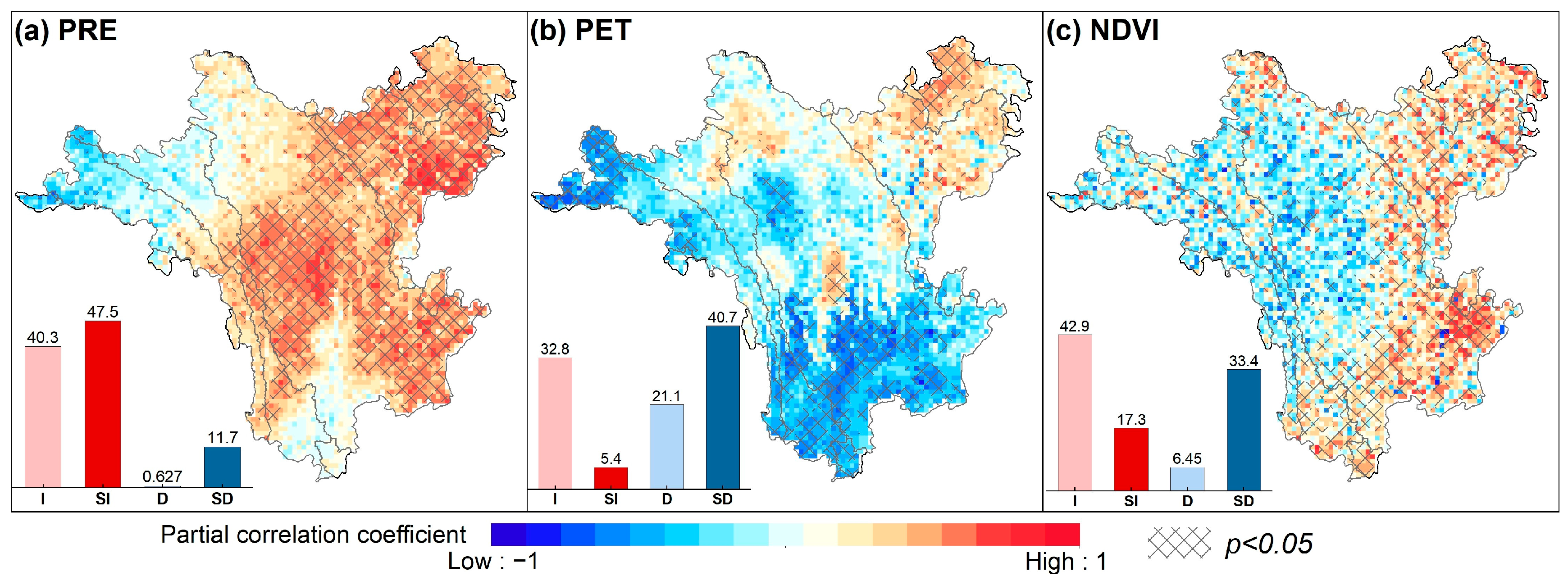
3.4.1. Correlation Analysis Between TWSAs and Regional Factors

Figure 7 presents the spatial distribution of the correlation coefficients calculated between TWSAs and PRE, PET, and the NDVI. TWSAs exhibited a positive correlation with variations in PRE across the HDM region. Specifically, significant positive and negative correlation areas covered 50.19% and 2.89% of the region, respectively. Approximately 47.5% of the area showed a non-significant positive correlation between PRE and TWSAs, while 11.7% exhibited a non-significant negative correlation. Spatially, the positive correlations between TWSAs and PRE were primarily concentrated in the central and eastern parts of the study area, whereas the negative correlations were mainly observed in the western part.
In general, PET and TWSAs showed significant negative correlations, concentrated in the northwest and south of the study area, accounting for 40.7% of the total area. In contrast, positive correlations were observed in the northeast of the HDM region, accounting for only 5.4% of the area.
The NDVI and TWSAs displayed a significant positive correlation in the southeastern part of the study area, accounting for ~17.3% of the total area, while a significant negative correlation was observed in the western part, covering ~33.4% of the area.
Overall, the correlation between climate factors (PRE and PET) and TWSAs was stronger than that of the NDVI.

3.4.2. Wavelet Coherence Between TWSAs and Global Environmental Factors

To investigate the impact of global environmental factors on TWSAs, we employed the WCA method (Figure 8). The coherence between TWSAs and the ENSO (Figure 8a) is intermittent but significant across multiple time scales. Strong coherence was observed at periods of 26–34 years, particularly during the El Niño events of 2005–2011, suggesting that ENSO exerts a notable influence on TWSAs during these periods. However, the coherence is not consistently significant throughout the study period, indicating that ENSO’s impact on TWSAs is phase-dependent and modulated by other climatic factors. The coherence between TWSAs and the PDO (Figure 8b) exhibits a more complex pattern, with significant correlations appearing at decadal scales (8–12 years). This suggests that PDO may play a role in modulating long-term TWSA variability. The analysis of TWSAs and the NAO (Figure 8c) shows significant coherence at shorter time scales (1–3 years), particularly during the mid-2010s. The coherence between TWSAs and the AO (Figure 8d) is relatively weak and sporadic, with significant correlations appearing only at specific time intervals and scales. This further underscores the limited and likely indirect influence of AO on TWSAs.
These findings suggest that the influence of global environmental factors on TWSAs is limited and likely indirect, with regional factors playing a more dominant role in shaping TWSA variability.

3.4.3. Relationships Between TWSAs and Regional and Global Drivers at Yearly and Seasonal Scales

Pearson correlation heatmaps illustrating the relationships between TWSAs and various driving factors are presented in Figure 9. The annual correlation matrix reveals that TWSAs are significantly positively correlated with PRE (r = 0.59, p < 0.001), PET (r = 0.44, p < 0.001), and the NDVI (r = 0.77, p < 0.001). In contrast, among the examined global environmental factors, only the NAO showed a statistically significant correlation with TWSAs (r = −0.19, p < 0.01). Among all global factors, NAO exhibited significant negative correlations with PET (r = −0.32, p < 0.001), PRE (r = −0.29, p < 0.001), and the NDVI (r = −0.25, p < 0.001), highlighting its potential to indirectly influence TWSAs through teleconnections by modulating regional-scale factors.
Seasonal correlation patterns differ from the annual patterns, indicating the influence of seasonal climate variability on these relationships. For example, in spring, the TWSAs show a stronger positive correlation with the NDVI (r = 0.40, p < 0.05) compared to the annual average, while during summer, they exhibit a significant negative correlation with PRE (r = −0.47, p < 0.05), which is not observed annual scale. The relationship between TWSAs and the ENSO, which is insignificant on an annual scale, becomes significantly positive in summer (r = 0.63, p < 0.01). NAO and AO appear to exert significant indirect effects on TWSA during winter by modulating PRE and PET. These findings highlight the complex interactions between climate variability and TWSAs.

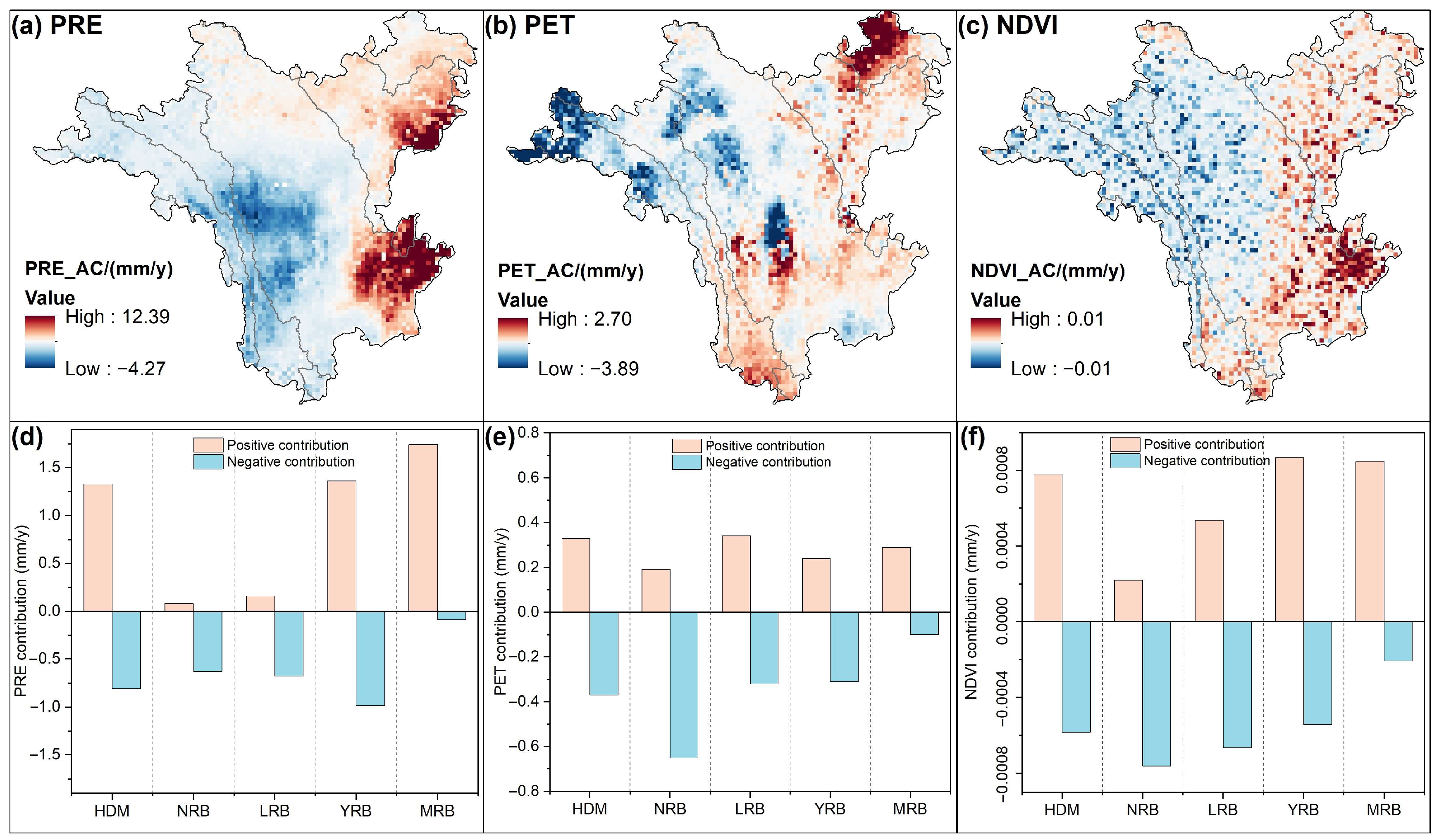
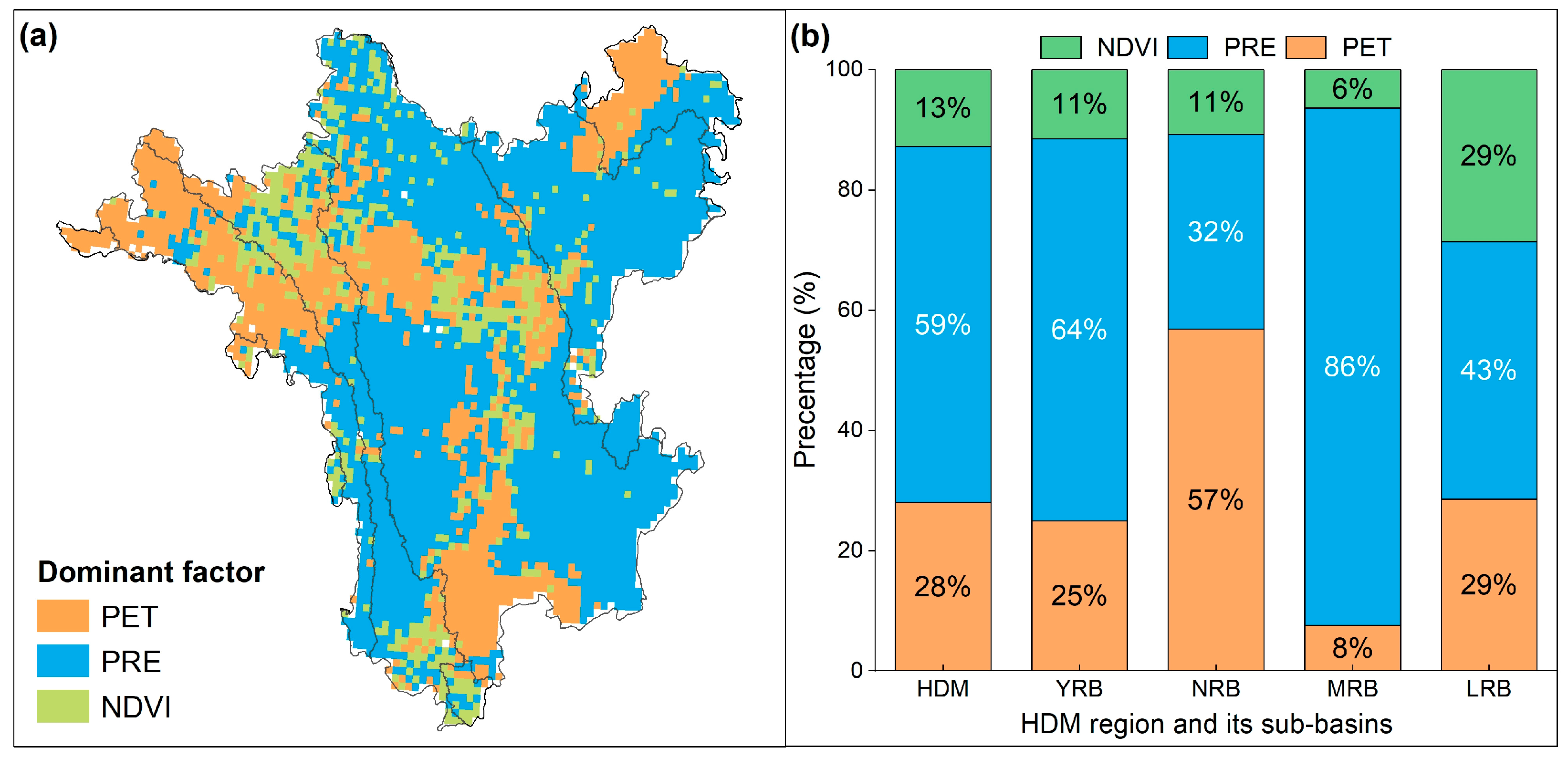
3.4.4. Contribution of Driving Factors to TWSAs and Dominant Factors

Based on the preceding analysis, it is evident that the influence of global environmental factors on TWSAs is relatively limited compared to regional factors and is primarily mediated through their effects on regional factors. This section analyzes the contributions of regional-scale factors to TWSAs, aiming to further identify their dominant controlling factors. Figure 10 illustrates the actual contribution of each environmental driver to the interannual trend variation in TWSAs, which follows the following order: PRE (0.52 mm/y) > PET (0.04 mm/y) > NDVI (1.97E-04 mm/y). PRE exhibits the largest actual contribution to TWSAs, with its average positive contribution (1.33 mm/y) exceeding its negative contribution (−0.81 mm/y). The MRB and YRB in the eastern part of the HDM region show positive contributions, reaching up to 12 mm/y in certain areas. In contrast, the NRB and LRB in the southwestern part of the HDM region exhibit negative contributions, averaging approximately −4.27 mm/y. Notably, PRE in the northwestern part of the HDM region shows a relatively small actual contribution to TWSAs. PET demonstrates a negative contribution (−0.37 mm/y) to TWSAs, which is larger than its positive contribution (0.33 mm/y), with high spatial heterogeneity. The western part of the study area, particularly the northern NRB, shows a significant negative contribution of approximately −3 mm/y. Conversely, the northeastern part of the MRB exhibits a positive contribution of ~2.7 mm/y. Additionally, the central and northern parts of the LRB show a negative contribution of −3 mm/y. The overall contribution of the NDVI to TWSAs is minimal, ranging from −0.01 to 0.01 mm/y. Positive contributions are observed in the eastern part of the HDM region, including the LRB and YRB, while negative contributions are concentrated in the western part, encompassing the NRB and LRB.
In terms of spatial mean statistics for each sub-basin, negative contributions of each driver to TWSAs are greater than the positive contributions in the NRB and LRB. In contrast, the positive contributions dominate in the YRB and MRB.
Thus, PRE exerts a greater influence than PET and the NDVI on TWSAs across the HDM region.
The dominant factor affecting TWSAs was determined by evaluating the relative contributions of PRE, PET, and the NDVI within each grid cell. PRE emerged as the primary driver, controlling > 59% of the TWSAs, particularly in the eastern and southwestern regions of the HDM region (Figure 11). PET accounted for ~28% of the TWSA variability, forming distinct strip-like patterns in the central and southwestern areas. In contrast, the NDVI exhibited a sporadic distribution in the central region, representing a relatively small proportion of only 13%.
At the sub-basin level, PRE dominated the TWSAs in the MRB (86%) and YRB (64%). Conversely, PET was the primary driver of TWSAs in the NRB (57%). The LRB showed a relatively higher influence of the NDVI (29%) compared to other basins. As both PET and PRE are climate-related factors, these findings highlight the critical role of regional climatic factors in shaping TWSA dynamics in the HDM region.

3.5. Assessment of Wet–Dry Characteristics for TWSAs in the HDM Region

The GRACE-DSI values exhibit significant temporal variability in the HDM region and its sub-basins from 2003 to 2022, reflecting alternating periods of drought and wetness (Figure 12). Overall, it shows a decreasing trend, with a rate of decline of −0.001 mm/y (p < 0.05). According to the drought level criteria (Table 2), lower DSI values indicate more severe drought conditions. Two mild drought events were identified during the study period: in 2006–2008 and 2010–2013. However, in most years, the DSI values ranged between −1.5 and 1.5, with the maximum value of 1.71 occurring in March 2005 and the minimum value of −1.47 in March 2010. These results suggest that the HDM region did not experience severe drought conditions except for isolated years.
At the sub-basin level, the GRACE-DSI analysis revealed significant spatial heterogeneity in TWSA dynamics. The MRB exhibited a fluctuating yet statistically significant upward trend (slope = 0.008, p < 0.05), indicating a transition from drier to wetter conditions. In contrast, the other sub-basins showed downward trends in the DSI, reflecting a shift towards drier conditions. The NRB experienced the most pronounced decline (slope = −0.011, p < 0.05), with drought conditions reaching the D3 level in certain months (e.g., May 2021, September 2022). The LRB also displayed a substantial decline in GRACE-DSI (Slope = −0.007, p < 0.01). However, the YRB exhibited a more moderate downward trend (slope = −0.001, p < 0.01), consistent with the overall trend observed for the entire HDM region.

4. Discussion

4.1. Discrepancies and Concordance in GRACE-Derived TWSA Products in the HDM Region

This study employed the high-resolution HWSA dataset [19] from GRACE observations to analyze TWSAs across the HDM region. The reliability of GRACE-based TWSA estimates has been well-established through validation against the in situ measurements in diverse climatic regions, ranging from tropical (Ethiopia [62]) to temperate (Poland) and Arctic (Sweden) zones [63]. These validation studies consistently report high correlation coefficients, confirming that the HWSA product accurately captures seasonal TWSA dynamics. While our analysis reveals strong agreement in trend patterns between HWSA and other GRACE-derived products (CSR, JPL, and GSFC), notable discrepancies emerged post-2008. The period from 2011 to 2022 showed particularly pronounced differences, with the GSFC estimates being systematically lower than other datasets (Figure 2). These inconsistencies may be attributed to the differences in GRACE data processing algorithms, de-stripping filters, Glacial Isostatic Adjustment corrections, leakage error corrections, and downscaling techniques [32]. Additionally, extreme weather events (e.g., droughts and floods) and human activities (e.g., groundwater extraction and coal mining) after 2011 may have significantly impacted TWSAs, with the GSFC data potentially responding differently to these events.
Despite these discrepancies, the overall agreement between the datasets supports the use of HWSA for monitoring TWSAs in the HDM region. These findings align with previous studies [10,32] and underscore the importance of considering the limitations of each data source and using multiple data sources to validate the TWSA estimates.

4.2. Underlying Driving Mechanisms of TWSAs in the HDM Region

Changes in TWSAs are influenced by a combination of global and regional environmental and climatic factors. The observed decline in TWSAs in the HDM region aligns with earlier findings by Xu et al. (2019) [10], Yang et al. (2023) [59], and Hua et al. (2024) [13] in southwestern China. Additionally, more pronounced declining trends have also been observed globally in South Korea [64] and India [65]. This decline could threaten the sustainability of surface and subsurface water resources in areas, with particularly concerning examples observed in the NBR and LRB within the HDM region. This study, using the GRACE-DSI to identify drought years in the HDM region, found a strong agreement with drought years identified by Wang et al. (2015) [66] in Southwest China. Specifically, the drought events of summer 2006, October 2009 to March 2010, and summer 2011 were identified, as illustrated in Figure 12. However, Deng et al. (2018) [67] reported an increase in TWSAs in specific areas within the Tibetan Plateau region, a trend that aligns with the findings from the eastern part (e.g., YRB and MRB) of the HDM in this study. The accumulation of TWSAs in these areas, driven by increased surface water, could lead to lake spillovers, thereby increasing the risks of floods and debris flows [29]. This pattern is explained by the similar spatial trends between TWSAs and PRE in the eastern part of the HDM region (Figure 3 and Figure 6a), where they also exhibit high partial correlation coefficients (Figure 7a).
TWSAs exhibit marked seasonal variability, largely driven by the hydrological cycle [5]. During the summer–autumn monsoon period, i.e., the primary wet season, TWSAs increase due to the combined effects of abundant PRE and enhanced surface runoff. In contrast, the winter–spring dry season presents a paradoxical hydrological regime. Despite reduced PRE and low river discharge, sustained vegetation transpiration continues to extract groundwater reserves. The rise in TWSAs (a positive TWSA trend) during the spring (March–May) and winter (December–February) months is primarily driven by snowmelt and increased PRE, as emphasized by Deng et al. (2018) [67] and Wang et al. (2020) [29].
Climate change and human activities are the primary drivers of TWSAs, though their relative influences vary significantly across different regions and climate zones. For instance, in northern India, TWSAs are predominantly driven by rainfall variability and groundwater extraction [65]. The Arabian Gulf faces a persistent water deficit due to extreme evaporation rates [68]. In the Mississippi River region, the fastest decline in groundwater has been attributed to intensive groundwater-based soybean farming [69]. While our study identifies climate factors as the primary source of TWSAs in the study area (Figure 11), the increase in PET signifies heightened atmospheric water demand. For instance, PET has been shown to affect TWSAs in 39.8% of global regions [8]. This accelerates the evaporation of surface water and soil moisture, thereby reducing water availability for groundwater recharge and surface water storage. Evidence suggests that the P/PET ratio plays a major role in shaping the temporal trends of soil moisture [70,71]. When PET exceeds PRE, the effectiveness of rainfall in recharging water resources is significantly diminished, leading to a decline in TWSAs. This mechanism explains the negative correlation between the PET and TWSAs observed in the southern and western parts of the HDM region. Conversely, when PRE surpasses PET, water is more likely to accumulate on the surface or infiltrate into the ground, resulting in an increase in TWSAs. This dynamic accounts for the positive correlation between PET and TWSAs in the northern HDM region (Figure 7b). Additionally, a high PET enhances vegetation transpiration, further reducing water availability for other hydrological processes and thus impacting TWSAs.
Vegetation plays a pivotal role in linking atmospheric, soil, and hydrological processes. Its structure (e.g., root depth) and activity (e.g., transpiration) directly influence soil moisture dynamics and groundwater recharge, serving as a critical driver of TWSAs [8,23]. However, the relationship between TWSAs and vegetation indices shows distinct zonal patterns. For example, Wang et al. (2025) [72] found that positive correlations dominate in tropical regions, whereas negative responses prevail at higher latitudes (north of 30°N) and in South American rainforests. In our study, significant vegetation greening in the eastern HDM region was associated with increased TWSAs (Figure 7). This positive relationship arises from the region’s warm climate, high solar radiation, and distinct seasonal precipitation patterns, which collectively enhance soil moisture retention by reducing evaporation and improving moisture storage capacity. Additionally, vegetation root systems promoted water infiltration and groundwater recharge, further augmenting TWSAs. Conversely, in the high-altitude western HDM region, where temperature and solar radiation limit vegetation growth, increases in the NDVI corresponded with TWSA reductions. This inverse relationship reflects greater plant water consumption under environmental constraints [73]. However, the contribution of the NDVI changes to TWSAs was relatively small (Figure 10), which can be explained by several factors: First, the effect of vegetation activity (as indicated by the NDVI) on TWSAs is primarily mediated through transpiration. Even if the NDVI indicates healthy vegetation, insufficient PRE or soil water saturation can still lead to a decline in TWSAs. Second, due to the gradual process of vegetation development, which requires the accumulation of adequate biomass and water resources, the impact of the NDVI on TWSAs often exhibits a time lag, which may be masked by other dominant hydrological factors, such as PRE variability, evaporation rates, and groundwater dynamics. Vegetation change significantly influences the land–water conditions by directly regulating evapotranspiration and indirectly affecting precipitation, runoff, and soil moisture through water cycle modifications. For instance, studies indicate that global greening increased evapotranspiration by 12 ± 2.4 mm/y and precipitation by 12.1 ± 2.7 mm/y from 1982 to 2011 [74]. These interconnected processes collectively diminish the direct and immediate influence of the NDVI on TWSAs, explaining its relatively minor contribution.
The high correlations between TWSAs and ENSO observed at the global scale [9] and within the La Plata Basin [75] underscore the significant influence of these climate modes. Guo et al. (2021) [34] further demonstrated that ENSO, PDO, the Atlantic Multidecadal Oscillation, and IOD exerted detectable effects on TWSAs across 76.5%, 74.6%, 59.7%, and 46.4% of global land areas, respectively. In the HDM region, our findings reveal a complex interplay of these global climate modes on TWSAs. Notably, among the examined global climate modes, PDO exhibits the strongest correlation with TWSAs, making it the primary global influence driver in this region. This result aligns well with previous studies by Chang et al. (2020) [20] and Scanlon et al. (2022) [7], further emphasizing the dominant role of PDO in modulating regional hydrological variability, including TWSAs. Furthermore, we identified a ~32-year cycle in the relationship between TWSAs and both ENSO and PDO, suggesting long-term climatic modulation of water storage dynamics. However, the linkages between the AO/NAO and TWSAs are weaker than expected, possibly due to topographic filtering by the HDM, which results in a unique regional response to Arctic oscillations. The coherence between these climate models and TWSAs is not consistently significant throughout the study period, indicating that their influence is phase-dependent and modulated by other climatic factors.

4.3. Uncertainties and Limitations

TWSAs comprise multiple components (e.g., groundwater storage, soil moisture, and surface water), making it challenging to validate each component individually at the regional scale due to the scarcity of adequate in situ observations of GWS. Although Chen et al. (2019) [39] attempted to validate the GWS component derived from GRACE using ground-based measurements, establishing observation networks in high-altitude regions faces significant difficulties due to complex terrain, harsh climatic conditions, and limited infrastructure. This lack of observational data introduces uncertainties into the accuracy of TWSA estimates, particularly in mountainous areas where such uncertainties may be more pronounced. Therefore, future research should focus on optimizing observation networks and integrating multi-source data (e.g., remote sensing and model simulations) to enhance the precision and reliability of TWSA estimates.
While numerous factors drive TWSAs, their influences are not isolated. Atmospheric circulation and complex physical processes often mediate relationships and interdependencies among these drivers. However, a singular focus on individual drivers or simplified mediation can limit our understanding of the complex, nonlinear interactions between above- and below-ground processes. Furthermore, despite the NDVI being a widely accepted proxy for vegetation productivity and capturing vegetation density and coverage, it has inherent limitations. For instance, the NDVI may saturate high vegetation densities, potentially limiting its ability to fully capture certain vegetation changes [76]. To further improve analyses, integrating complementary vegetation indices, such as the leaf area index (LAI) and the kernel normalized difference vegetation index (kNDVI), along with soil moisture data (e.g., from the Soil Moisture Active Passive (SMAP) mission) would improve differentiation between water-stress-induced vegetation changes and those driven by other factors. Moreover, advancing research on TWSAs in the HDM region requires a stronger focus on meteorological and atmospheric circulation factors, particularly precipitation dynamics, to better elucidate the underlying mechanisms of TWSAs.
Although this study employed high-resolution downscaled GRACE products to analyze the spatial patterns of soil water storage changes, the original GRACE data have a spatial resolution of 0.25°, leading to relatively lower accuracy at the local scale. Therefore, a further downscaling of GRACE data is required to obtain higher-precision results and more accurately reflect the changes in water storage. Additionally, integrating advanced modeling techniques and higher-resolution remote sensing data could help to mitigate these limitations and improve the robustness of TWSA estimates.

5. Conclusions

This study investigates the TWSA response to climate change, both regional and global environmental factors. Using high-spatiotemporal-resolution GRACE data from 2003 to 2022, we applied wavelet coherence analysis and multiple linear regression to examine the spatiotemporal dynamics of TWSA. The main conclusions are as follows:
(1) Amidst the impacts of global climate change, TWSAs in the HDM region declined at a rate of approximately −2.83 mm/y from 2003 to 2022, with fluctuations becoming more pronounced. Significant regional differences were observed in the TWSA trends: TWSAs increased in the west but decreased in the east. The largest decline occurred in the NRB (−17.17 mm/y, p < 0.01), while the MRB showed a significant upward trend (3.24 mm/y, p < 0.01). TWSAs also exhibited distinct seasonal fluctuations, with the most substantial decrease occurring during winter and spring.
(2) Regional factors, rather than global influences, were the primary drivers of TWSA variability in the HDM region. PRE dominated the TWSA variability (59%), particularly in the eastern and southwestern areas, while PET contributed 28%, forming distinct strip-like patterns in the central-southwestern regions, and the NDVI showed a sporadic central distribution, accounting for only 13%. Although global environmental factors did not directly influence it, the NAO exhibited a significant negative correlation with TWSAs (r = −0.19, p < 0.01), primarily mediated through its effect on PET (r = −0.56, p < 0.05) during winter.
(3) The GRACE-DSI in the HDM region showed a decreasing trend at a rate of −0.001 mm/y (p < 0.05) under climate change. The NRB experienced the most pronounced decline (slope = −0.011, p < 0.05), with drought conditions reaching extreme levels in certain months. In contrast, the MRB exhibited a fluctuating transition from drier to wetter conditions (DSI slope = 0.008, p < 0.05).
This study, in summary, offers important insights into the evolutionary patterns and underlying drivers of TWSAs within the HDM region. This assessment further demonstrates that TWSAs critically regulate dry–wet transitions, linking large-scale hydrological changes to regional climate dynamics. These findings highlight the critical role of regional climate factors in driving TWSA and underscore the need for targeted water resource management strategies to address the challenges posed by climate change.

Supplementary Materials

The following supporting information can be downloaded at: https://www.mdpi.com/article/10.3390/rs17142447/s1, Figure S1: Temporal trends of the TWSAs driving factors in the HDM region and its sub-basins (a) Precipitation (PRE), (b) Potential evapotranspiration (PET), (c) Normalized Difference Vegetation Index (NDVI); Figure S2: Spatial distribution of the mean TWSAs driving factors in the HDM region and its sub-basins (2003−2022) (a) PRE, (b) PET, (c) NDVI; Figure S3: Temporal variations of ocean-atmosphere climate, including: (a) PDO, (b)ENSO, (c) NAO, and (d) AO from 2003 to 2022.

Author Contributions

X.L.: Writing—original draft, writing—review and editing, software, project administration, conceptualization, and funding acquisition. Y.X.: Writing—review and editing, validation, and methodology. D.W.: software, methodology, investigation, and data curation. S.T.: Investigation and methodology. X.C.: Investigation and formal analysis. W.Z.: Investigation and formal analysis. All authors have read and agreed to the published version of the manuscript.

Funding

This research was funded by the Startup Project of Doctoral Research by China West Normal University (Grant No. 24KE005).

Data Availability Statement

The materials and data used in the present manuscript are available upon request to the corresponding author.

Acknowledgments

The authors gratefully acknowledge the editor and three anonymous reviewers for their valuable feedback and constructive suggestions, which have significantly improved the quality and clarity of this manuscript.

Conflicts of Interest

The authors declare no conflicts of interest.

References

  1. Rodell, M.; Famiglietti, J.S.; Wiese, D.N.; Reager, J.T.; Beaudoing, H.K.; Landerer, F.W.; Lo, M.H. Emerging trends in global freshwater availability. Nature 2018, 557, 651–659. [Google Scholar] [CrossRef]
  2. Abbott, B.W.; Bishop, K.; Zarnetske, J.P.; Minaudo, C.; Chapin, F.S., III; Krause, S.; Hannah, D.M.; Conner, L.; Ellison, D.; Godsey, S.E.; et al. Human domination of the global water cycle absent from depictions and perceptions. Nat. Geosci. 2019, 12, 533–540. [Google Scholar] [CrossRef]
  3. Chao, N.; Jin, T.; Cai, Z.; Chen, G.; Liu, X.; Wang, Z.; Yeh, P.J. Estimation of component contributions to total terrestrial water storage change in the Yangtze river basin. J. Hydrol. 2021, 595, 125661. [Google Scholar] [CrossRef]
  4. Liu, M.; Pei, H.; Shen, Y. Evaluating dynamics of GRACE groundwater and its drought potential in Taihang Mountain Region, China. J. Hydrol. 2022, 612, 128156. [Google Scholar] [CrossRef]
  5. Wu, C.; Yeh, P.J.; Yao, T.; Gong, Z.; Niu, J.; Yuan, S. Controls of climate seasonality and vegetation dynamics on the seasonal variability of terrestrial water storage under diverse climate regimes. Water Resour. Res. 2025, 61, e2024WR038065. [Google Scholar] [CrossRef]
  6. Padrón, R.S.; Gudmundsson, L.; Decharme, B.; Ducharne, A.; Lawrence, D.M.; Mao, J.; Peano, D.; Krinner, G.; Kim, H.; Seneviratne, S.I. Observed changes in dry-season water availability attributed to human-induced climate change. Nat. Geosci. 2020, 13, 477–481. [Google Scholar] [CrossRef]
  7. Scanlon, B.R.; Rateb, A.; Anyamba, A.; Kebede, S.; MacDonald, A.M.; Shamsudduha, M.; Small, J.; Sun, A.; Taylor, R.G.; Xie, H. Linkages between GRACE water storage, hydrologic extremes, and climate teleconnections in major African aquifers. Geophys. Res. Lett. 2022, 17, 014046. [Google Scholar] [CrossRef]
  8. Lu, J.; Kong, D.; Zhang, Y.; Xie, Y.; Gu, X.; Gulakhmadov, A. Hotspots of global water resource changes and their causes. Earths Future 2025, 13, e2024EF005461. [Google Scholar] [CrossRef]
  9. Ni, S.; Chen, J.; Wilson, C.R.; Li, J.; Hu, X.; Fu, R. Global terrestrial water storage changes and connections to ENSO events. Surv. Geophys. 2018, 39, 1–22. [Google Scholar] [CrossRef]
  10. Xu, L.; Chen, N.; Zhang, X.; Chen, Z. Spatiotemporal changes in China’s terrestrial water storage from GRACE satellites and its possible drivers. J. Geophys. Res. Atmos. 2019, 124, 11976–11993. [Google Scholar] [CrossRef]
  11. Liu, B.; Zou, X.; Yi, S.; Sneeuw, N.; Cai, J.; Li, J. Identifying and separating climate- and human-driven water storage anomalies using grace satellite data. Remote Sens. Environ. 2021, 263, 112559. [Google Scholar] [CrossRef]
  12. Swenson, S.; Yeh, P.J.F.; Wahr, J.; Famiglietti, J. A comparison of terrestrial water storage variations from GRACE with in situ measurements from Illinois. Geophys. Res. Lett. 2006, 33, L16401. [Google Scholar] [CrossRef]
  13. Hua, S.; Jing, H.; Qiu, G.; Kuang, X.; Andrews, C.B.; Chen, X.; Zheng, C. Long-term trends in human-induced water storage changes for China detected from GRACE data. J. Environ. Manag. 2024, 368, 122253. [Google Scholar] [CrossRef]
  14. Tapley, B.D.; Watkins, M.M.; Flechtner, F.; Reigber, C.; Bettadpur, S.; Rodell, M.; Sasgen, I.; Famiglietti, J.S.; Landerer, F.W.; Chambers, D.P.; et al. Contributions of GRACE to understanding climate change. Nat. Clim. Change 2019, 9, 358–369. [Google Scholar] [CrossRef]
  15. Long, D.; Shen, Y.; Sun, A.; Yang, H.; Longuevergne, L.; Yang, Y.; Li, B.; Chen, L. Drought and flood monitoring for a large karst plateau in Southwest China using extended GRACE data. Remote Sens. Environ. 2014, 155, 145–160. [Google Scholar] [CrossRef]
  16. Humphrey, V.; Gudmundsson, L.; Seneviratne, S.I. Assessing global water storage variability from GRACE: Trends, seasonal cycle, subseasonal anomalies and extremes. Surv. Geophys. 2016, 37, 357–395. [Google Scholar] [CrossRef]
  17. Ali, S.; Liu, D.; Fu, Q.; Cheema, M.J.; Pham, Q.B.; Rahaman, M.M.; Dang, D.D.; Anh, D.T. Improving the resolution of GRACE data for spatio-temporal groundwater storage assessment. Remote Sens. 2021, 13, 3513. [Google Scholar] [CrossRef]
  18. Nourani, V.; Paknezhad, N.J.; Ng, A.; Wen, Z.; Dabrowska, D.; Üzelaltınbulat, S. Application of the machine learning methods for GRACE data based groundwater modeling, a systematic review. Groundw. Sustain. Dev. 2024, 25, 101113. [Google Scholar] [CrossRef]
  19. Zhang, G.; Xu, T.; Yin, W.; Bateni, S.M.; Jun, C.; Kim, D.; Liu, S.; Xu, Z.; Ming, W.; Wang, J. A machine learning downscaling framework based on a physically constrained sliding window technique for improving resolution of global water storage anomaly. Remote Sens. Environ. 2024, 313, 114359. [Google Scholar] [CrossRef]
  20. Chang, L.L.; Yuan, R.; Gupta, H.V.; Winter, L.; Niu, G. Why is the terrestrial water storage in dryland regions declining? A perspective based on gravity recovery and climate experiment satellite observations and Noah land surface model with multiparameterization schemes model simulations. Water Resour. Res. 2020, 56, e2020WR027102. [Google Scholar] [CrossRef]
  21. Mo, X.; Wu, J.; Wang, Q.; Zhou, H. Variations in water storage in China over recent decades from GRACE observations and GLDAS. Nat. Hazards Earth Syst. Sci. 2016, 16, 469–482. [Google Scholar] [CrossRef]
  22. Shi, X.; Wang, Y.; Mao, J.; Thornton, P.E.; Ricciuto, D.M.; Hoffman, F.M.; Hao, Y. Quantifying the long-term changes of terrestrial water storage and their driving factors. J. Hydrol. 2024, 635, 131096. [Google Scholar] [CrossRef]
  23. Trautmann, T.; Koirala, S.; Carvalhais, N.; Güntner, A.; Jung, M. The importance of vegetation in understanding terrestrial water storage variations. Hydrol. Earth Syst. Sci. 2022, 26, 1089–1109. [Google Scholar] [CrossRef]
  24. Li, B.; Rodell, M.; Save, H. Terrestrial water storage in 2024. Nat. Rev. Earth Environ. 2025, 6, 261–263. [Google Scholar] [CrossRef]
  25. Chen, A.; Xiong, J.; Wu, S.; Yang, Y. Changes in terrestrial water storage in the Three-North region of China over 2003–2021: Assessing the roles of climate and vegetation restoration. J. Hydrol. 2024, 637, 131303. [Google Scholar] [CrossRef]
  26. Meng, F.; Su, F.; Li, Y.; Tong, K. Changes in terrestrial water storage during 2003–2014 and possible causes in Tibetan Plateau. J. Geophys. Res. Atmos. 2019, 124, 2909–2931. [Google Scholar] [CrossRef]
  27. Xu, G.; Wu, Y.; Liu, S.; Chen, S.; Zhang, Y.; Pan, Y.; Wang, L.; Dokuchits, E.Y.; Nkwazema, O.C. How 2022 extreme drought influences the spatiotemporal variations of terrestrial water storage in the Yangtze River Catchment: Insights from GRACE-based drought severity index and in-situ measurements. J. Hydrol. 2023, 626, 130245. [Google Scholar] [CrossRef]
  28. Shen, X.; Niu, L.; Jia, X.; Yang, T.; Hu, W.; Chu, J.; Biswas, A.; Shao, M. Disentangling ecological restoration’s impact on terrestrial water storage. Geophys. Res. Lett. 2025, 52, e2024GL111669. [Google Scholar] [CrossRef]
  29. Wang, J.; Chen, X.; Hu, Q.; Liu, J. Responses of terrestrial water storage to climate variation in the Tibetan Plateau. J. Hydrol. 2020, 584, 124652. [Google Scholar] [CrossRef]
  30. Nie, N.; Zhang, W.; Chen, H.; Guo, H. A Global Hydrological Drought Index Dataset Based on Gravity Recovery and Climate Experiment (GRACE) Data. Water Resour Manag. 2018, 32, 1275–1290. [Google Scholar] [CrossRef]
  31. Liu, Q.; Zhang, X.; Xu, Y.; Li, C.; Zhang, X.; Wang, X. Characteristics of groundwater drought and its correlation with meteorological and agricultural drought over the North China Plain based on GRACE. Ecol. Indic. 2024, 161, 111925. [Google Scholar] [CrossRef]
  32. Zhao, J.; Li, G.; Zhu, Z.; Hao, Y.; Hao, H.; Yao, J.; Bao, T.; Liu, Q.; Yeh, T.J. Analysis of the spatiotemporal variation of groundwater storage in Ordos Basin based on GRACE gravity satellite data. J. Hydrol. 2024, 632, 130931. [Google Scholar] [CrossRef]
  33. Awange, J.L.; Forootan, E.; Kuhn, M.; Kusche, J.; Hech, B. Water storage changes and climate variability within the Nile Basin between 2002 and 2011. Adv. Water Resour. 2014, 73, 1–15. [Google Scholar] [CrossRef]
  34. Guo, L.; Li, T.; Chen, D.; Liu, J.; He, B.; Zhang, Y. Links between global terrestrial water storage and large-scale modes of climatic variability. J. Hydrol. 2021, 598, 126419. [Google Scholar] [CrossRef]
  35. Scanlon, B.R.; Fakhreddine, S.; Rateb, A.; Graaf, I.; Famiglietti, J.; Gleeson, T.; Grafton, R.Q.; Jobbagy, E.; Kebede, S.; Kolusu, S.R.; et al. Global water resources and the role of groundwater in a resilient water future. Nat. Rev. Earth Environ. 2023, 4, 87–101. [Google Scholar] [CrossRef]
  36. Li, Y.; Wang, Z.; Zhang, Y.; Li, X.; Huang, W. Drought variability at various timescales over Yunnan Province, China: 1961–2015. Theor. Appl. Climatol. 2019, 138, 743–757. [Google Scholar] [CrossRef]
  37. Cheng, Q.; Gao, L.; Zhong, F.; Zuo, X.; Ma, M. Spatiotemporal variations of drought in the Yunnan-Guizhou Plateau, southwest China, during 1960–2013 and their association with large-scale circulations and historical records. Ecol. Indic. 2020, 112, 106041. [Google Scholar] [CrossRef]
  38. Yang, W.; Jin, F.; Si, Y.; Li, Z. Runoff change controlled by combined effects of multiple environmental factors in a headwater catchment with cold and arid climate in northwest China. Sci. Total Environ. 2021, 756, 143995. [Google Scholar] [CrossRef]
  39. Chen, H.; Zhang, W.; Nie, N.; Guo, Y. Long-term groundwater storage variations estimated in the Songhua River Basin by using GRACE products, land surface models, and in-situ observations. Sci. Total Environ. 2019, 649, 372–387. [Google Scholar] [CrossRef]
  40. Yang, S.; Zhong, Y.; Wu, Y.; Yang, K.; An, Q.; Bai, H.; Liu, S. Quantifying long-term drought in China’s exorheic basins using a novel daily GRACE reconstructed TWSA index. J. Hydrol. 2025, 655, 132919. [Google Scholar] [CrossRef]
  41. Thomas, B.F.; Famiglietti, J.S.; Landerer, F.W.; Wiese, D.N.; Molotch, N.P.; Argus, D.F. GRACE groundwater drought index: Evaluation of California Central Valley groundwater drought. Remote Sens. Environ. 2017, 198, 384–392. [Google Scholar] [CrossRef]
  42. Shi, S.; Liu, G.; Li, Z.; Ye, X. Elevation-dependent growth trends of forests as affected by climate warming in the southeastern Tibetan Plateau. For. Ecol. Manag. 2021, 498, 119551. [Google Scholar] [CrossRef]
  43. Zhong, X.H.; Liu, S.Z. Theoryand Practice of Mountain Environment; Science Press: Beijing, China, 2015; pp. 163–174. [Google Scholar]
  44. Yang, J.; Dai, J.; Yao, H.; Tao, Z.; Zhu, M. Vegetation distribution and vegetation activity changes in the Hengduan Mountains from 1992 to 2020. Acta Geogr. Sin. 2022, 77, 2787–2802. [Google Scholar]
  45. Lu, E.; Luo, Y.; Zhang, R.; Wu, Q.; Liu, L. Regional atmospheric anomalies responsible for the 2009–2010 severe drought in China. J. Geophys. Res. Atmos. 2011, 116, D21114. [Google Scholar] [CrossRef]
  46. Wahr, J.; Molenaar, M.; Bryan, F. Time variability of the Earth’s gravity field: Hydrological and oceanic effects and their possible detection using GRACE. J. Geophys. Res. 1998, 103, 30205–30229. [Google Scholar] [CrossRef]
  47. Loomis, B.D.; Luthcke, S.B.; Sabaka, T.J. Regularization and error characterization of GRACE mascons. J. Geod. 2019, 93, 1381–1398. [Google Scholar] [CrossRef] [PubMed]
  48. Save, H.; Bettadpur, S.; Tapley, B.D. High-resolution CSR GRACE RL05 mascons. J. Geophys. Res. Solid Earth 2016, 121, 7547–7569. [Google Scholar] [CrossRef]
  49. Abatzoglou, J.T.; Dobrowski, S.Z.; Parks, S.A.; Hegewisch, K.C. TerraClimate, a high-resolution global dataset of monthly climate and climatic water balance from 1958–2015. Sci. Data 2018, 5, 170191. [Google Scholar] [CrossRef]
  50. Gao, J.; Shi, Y.; Zhang, H.; Shen, W.; Xiao, T.; Zhang, Y. China Regional 250 m Normalized Difference Vegetation Index Data Set (2000–2022); National Tibetan Plateau/Third Pole Environment Data Center: Beijing, China, 2023. [Google Scholar] [CrossRef]
  51. Zhao, J.; Huang, S.; Huang, Q.; Leng, G.; Wang, H.; Li, P. Watershed water-energy balance dynamics and their association with diverse influencing factors at multiple time scales. Sci. Total Environ. 2020, 711, 135189. [Google Scholar] [CrossRef]
  52. Li, B.; Yang, Y.; Li, Z. Combined effects of multiple factors on spatiotemporally varied soil moisture in China’s Loess Plateau. Agric. Water Manag. 2021, 258, 107180. [Google Scholar] [CrossRef]
  53. Zuo, J.; Ren, H.; Li, W.; Wang, L. Interdecadal Variations in the Relationship between the Winter North Atlantic Oscillation and Temperature in South-Central China. J. Clim. 2016, 29, 7477–7493. [Google Scholar] [CrossRef]
  54. Mantua, N.J.; Hare, S.R.; Zhang, Y.; Wallace, J.M.; Francis, R.C. A Pacific interdecadal climate oscillation with impacts on salmon production. Bull. Am. Meteorol. Soc. 1997, 78, 1069–1080. [Google Scholar] [CrossRef]
  55. Watkins, M.M.; Wiese, D.N.; Yuan, D.N.; Boening, C.; Landerer, F.W. Improved methods for observing Earth’s time variable mass distribution with GRACE using spherical cap mascons. J. Geophys. Res. Solid Earth 2015, 120, 2648–2671. [Google Scholar] [CrossRef]
  56. Mann, H.B. Nonparametric tests against trend. Econometrica 1945, 13, 245–259. [Google Scholar] [CrossRef]
  57. Kendall, M.G. Rank Correlation Methods; Charles Griffin: London, UK, 1975. [Google Scholar]
  58. Wang, F.; Lai, H.; Li, Y.; Feng, K.; Tian, Q.; Guo, W.; Qu, Y.; Yang, H. Spatio-temporal evolution and teleconnection factor analysis of groundwater drought based on the GRACE mascon model in the Yellow River Basin. J. Hydrol. 2023, 626, 130349. [Google Scholar] [CrossRef]
  59. Yang, B.; Li, Y.; Tao, C.; Cui, C.; Hu, F.; Cui, Q.; Meng, L.; Zhang, W. Variations and drivers of terrestrial water storage in ten basins of China. J. Hydrol. Reg. Stud. 2023, 45, 101286. [Google Scholar] [CrossRef]
  60. Gan, T.Y.; Gobena, A.K.; Wang, Q. Precipitation of southwestern Canada: Wavelet, scaling, multifractal analysis, and teleconnection to climate anomalies. J. Geophys. Res. Atmos. 2007, 112, D10110. [Google Scholar] [CrossRef]
  61. Zhao, M.; Geruo, A.; Velicogna, I.; Kimball, J.S. Satellite observations of regional drought severity in the continental united states using grace-based terrestrial water storage changes. J. Clim. 2017, 30, 6297–6308. [Google Scholar] [CrossRef]
  62. Yoshe, A.K. Water availability identification from GRACE dataset and GLDAS hydrological model over data-scarce river basins of Ethiopia. Hydrol. Sci. J. 2024, 69, 721–745. [Google Scholar] [CrossRef]
  63. Rzepecka, Z.; Birylo, M.; Jarsjö, J.; Cao, F.; Pietroń, J. Groundwater Storage Variations across Climate Zones from Southern Poland to Arctic Sweden: Comparing GRACE-GLDAS Models with Well Data. Remote Sens. 2024, 16, 2104. [Google Scholar] [CrossRef]
  64. Cho, Y. Analysis of terrestrial water storage variations in South Korea using GRACE satellite and GLDAS data in Google Earth Engine. Hydrol. Sci. J. 2024, 69, 1032–1045. [Google Scholar] [CrossRef]
  65. Rana, S.K.; Chamoli, A. GRACE-derived groundwater variability and its resilience in north India: Impact of climatic and socioeconomic factors. Hydrol. Sci. J. 2024, 69, 2159–2171. [Google Scholar] [CrossRef]
  66. Wang, L.; Chen, W.; Zhou, W.; Huang, G. Understanding and detecting super-extreme droughts in Southwest China through an integrated approach and index. Q. J. R. Meteorol. Soc. 2015, 142, 529–535. [Google Scholar] [CrossRef]
  67. Deng, H.; Pepin, N.C.; Liu, Q.; Chen, Y. Understanding the spatial differences in terrestrial water storage variations in the Tibetan Plateau from 2002 to 2016. Clim. Change 2018, 151, 379–393. [Google Scholar] [CrossRef]
  68. Boulahia, A.K.; García-García, D.; Trottini, M.; Sayol, J.-M.; Vigo, M.I. Hydrological Cycle in the Arabian Sea Region from GRACE/GRACE-FO Missions and ERA5 Data. Remote Sens. 2024, 16, 3577. [Google Scholar] [CrossRef]
  69. Dash, P.; Shekhar, S.; Paul, V.; Feng, G. Influence of Land Use and Land Cover Changes and Precipitation Patterns on Groundwater Storage in the Mississippi River Watershed: Insights from GRACE Satellite Data. Remote Sens. 2024, 16, 4285. [Google Scholar] [CrossRef]
  70. Cook, B.I.; Smerdon, J.E.; Seager, R.; Coats, S. Global warming and 21st century drying. Clim. Dyn. 2014, 43, 2607–2627. [Google Scholar] [CrossRef]
  71. Chen, X.; Su, Y.; Liao, J.; Shang, J.; Dong, T.; Wang, C.; Liu, W.; Zhou, G.; Liu, L. Detecting significant decreasing trends of land surface soil moisture in eastern China during the past three decades (1979–2010). Geophys. Res. Atmos. 2016, 121, 5177–5192. [Google Scholar] [CrossRef]
  72. Wang, C.; Cui, A.; Ji, R.; Huang, S.; Li, P.; Chen, N.; Shao, Z. Spatiotemporal Responses of Global Vegetation Growth to Terrestrial Water Storage. Remote Sens. 2025, 17, 1701. [Google Scholar] [CrossRef]
  73. Wei, Z.; Wan, X. Spatial and temporal characteristics of NDVI in the Weihe River Basin and its correlation with terrestrial water storage. Remote Sens. 2022, 14, 5532. [Google Scholar] [CrossRef]
  74. Zeng, Z.; Piao, S.; Li, L.Z.; Wang, T.; Ciais, P.; Lian, X.; Yang, Y.; Mao, J.; Shi, X.; Myneni, R.B. Impact of earth greening on the terrestrial water cycle. J. Clim. 2018, 31, 2633–2650. [Google Scholar] [CrossRef]
  75. Pereira, A.; Cornero, C.; Oliveira Cancoro de Matos, A.C.; Seoane, R.; Pacino, M.C.; Blitzkow, D. Assessing water storage variations in La Plata basin and sub-basins from GRACE, global models data and connection with ENSO events. Hydrol. Sci. J. 2024, 69, 1012–1031. [Google Scholar] [CrossRef]
  76. Huete, A.; Didan, K.; Miura, T.; Rodriguez, E.P.; Gao, X.; Ferreira, L.G. Overview of the radiometric and biophysical performance of the MODIS vegetation indices. Remote Sens. Environ. 2002, 83, 195–213. [Google Scholar] [CrossRef]
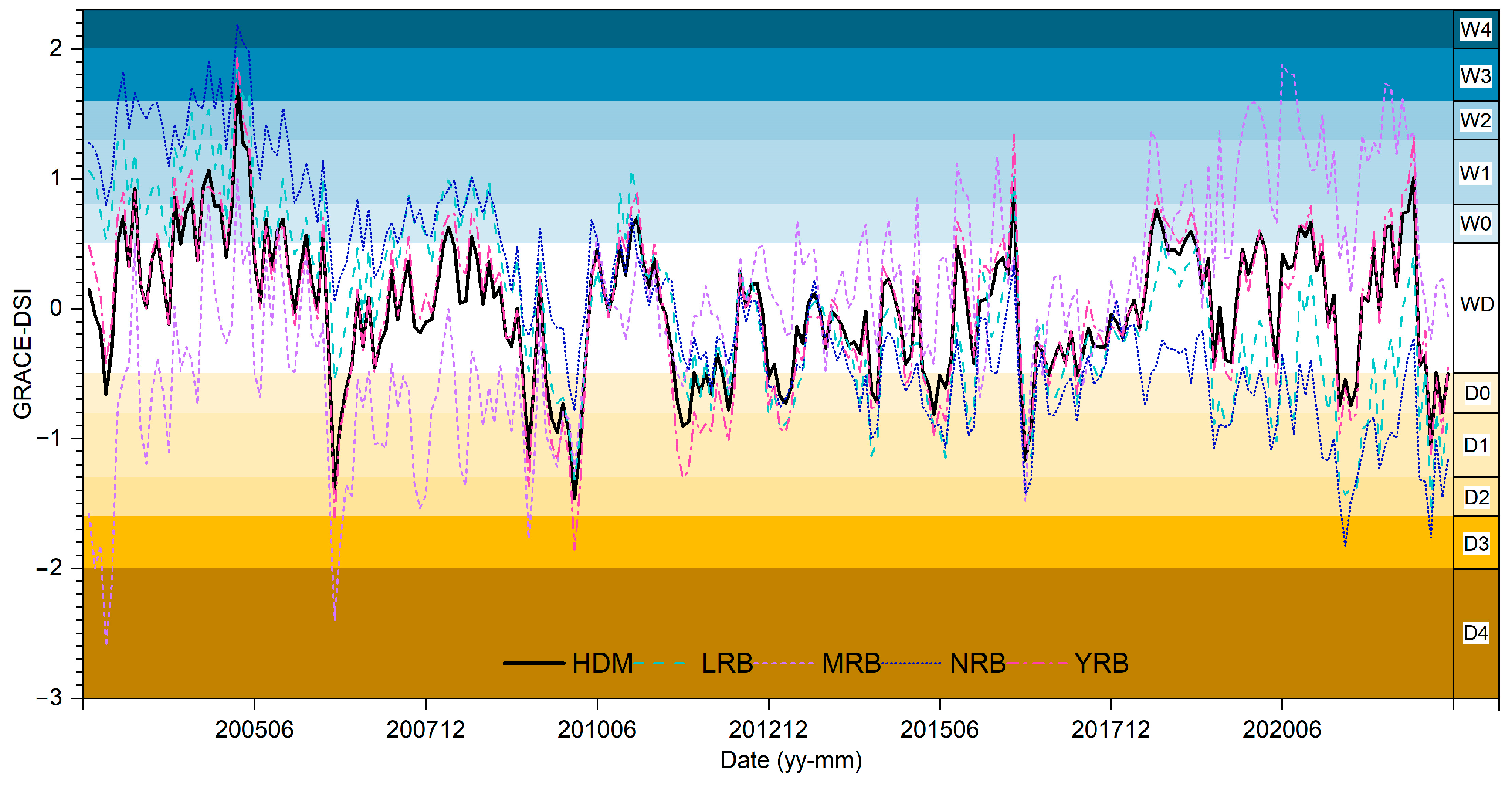
Figure 1. Overview of the study area. (a) Geographical location of the Hengduan Mountains region in China; (b) topography, river networks, and major drainage basins; (c) mean annual temperature (1979–2018); (d) mean annual precipitation (1979–2018); (e) land use/cover in 2020.
Remotesensing 17 02447 g001
Figure 2. Comparison of the TWSAs from HWSA and GRACE-derived datasets (CSR, JPL, and GSFC).
Remotesensing 17 02447 g002
Figure 3. Spatiotemporal variations in TWSAs in the HDM region and its sub-basins: (a) Spatial trend of TWSAs during the period 2003–2022; (b) temporal variations in TWSAs in the HDM region (c); Nujiang River basin (d); Lancang River basin (e); Min River basin (f); Yalong River Basin. The shaded areas in panels (bf) represent the standard deviation; ‘***’ indicates statistical significance at p < 0.001.
Remotesensing 17 02447 g003
Figure 4. Temporal variations in TWSA across the HDM region during 2003–2022: (a) monthly TWSA time series for individual years; (b) multi-year monthly mean TWSA values, and (c) seasonal mean TWSA values for spring, summer, autumn, and winter. ‘*’denotes statistical significance at p < 0.05, while ‘**’ indicates p < 0.01.
Remotesensing 17 02447 g004
Figure 5. Spatial patterns of mean TWSAs and their trends for each season (a) spring, (b) summer, (c) autumn, and (d) winter in the HDM region from 2003 to 2022. p-value indicating statistical significance. The inset plot in the lower left corner of each illustrates the seasonal mean TWSAs.
Remotesensing 17 02447 g005
Figure 6. Spatial trends and temporal slopes of key drivers for TWSAs in the HDM region (2003–2022): (ac) Spatial distribution of annual trends for (a) PRE, (b) PET, and (c) NDVI, p-value indicating statistical significance; (df) temporal slopes of (d) PRE, (e) PET, and (f) NDVI across the entire HDM region and its three sub-basins. “***” denotes statistical significance at p < 0.001.
Remotesensing 17 02447 g006
Figure 7. Correlation coefficients between TWSAs and (a) PRE, (b) PET, and (c) NDVI. Note: SI: significant increase (p < 0.05); I: insignificant increase (p > 0.05); D: insignificant decrease (p > 0.05); SD: significant decrease (p < 0.05); p-value indicating statistical significance.
Remotesensing 17 02447 g007
Figure 8. Wavelet coherence analysis between TWSAs and climate indices in the HDM region (2003–2022): (a) ENSO, (b) PDO, (c) NAO, and (d) AO. The color gradient from red to blue indicates decreasing coherence strength. The right-pointing horizontal arrows denote in-phase relationships, while the left-pointing arrows represent anti-phase relationships. Statistically significant regions (p < 0.05, red noise test) are enclosed by thick black contours. Edge effects are excluded from interpretation (thin black contours near boundaries).
Remotesensing 17 02447 g008
Figure 9. Pearson correlation coefficients between TWSAs and their potential drivers. Left panels present annual-scale correlations, while right panels display seasonal variations (spring, summer, autumn, winter).
Remotesensing 17 02447 g009
Figure 10. Actual contributions of PRE, PET, and the NDVI to annual TWSA trends across the HDM region from 2003 to 2022: (ac) Spatial patterns of the absolute contributions from PRE (a), PET (b), and NDVI (c). PRE_AC, PET_AC, and NDVI_AC denote the actual contributions of changes in PRE, PET, and NDVI to TWSAs, respectively; (df) average positive and negative contributions from PRE (d), PET (e), and NDVI (f) across the entire HDM region and its three sub-basins.
Remotesensing 17 02447 g010
Figure 11. Dominant drivers of TWSAs in the HDM region and its sub-basins: (a) Spatial distribution of the dominant factors influencing TWSAs; (b) relative contribution (%) of individual drivers to TWSA variability across the HDM region and its sub-basins.
Remotesensing 17 02447 g011
Figure 12. Temporal variations in GRACE-DSI in the HDM region and its sub-basins.
Remotesensing 17 02447 g012
Table 2. Categorization of GRACE-DSI.
CategoryDescriptionGRACE-DSICategoryDescriptionGRACE-DSI
W4Exceptionally wet≥2.0D0Abnormally dry−0.50–−0.79
W3Extremely wet1.60–1.99D1Moderate drought−0.80–−1.29
W2Very wet1.30–1.59D2Severe drought−1.30–−1.59
W1Moderately wet0.80–1.29D3Extreme drought−1.60–−1.99
W0Slightly wet0.50–0.79D4Exceptional drought≤−2.0
WDNear normal0.49–0.49
Disclaimer/Publisher’s Note: The statements, opinions and data contained in all publications are solely those of the individual author(s) and contributor(s) and not of MDPI and/or the editor(s). MDPI and/or the editor(s) disclaim responsibility for any injury to people or property resulting from any ideas, methods, instructions or products referred to in the content.

