Abstract
Land desertification represents a significant and sensitive global ecological issue. In the Inner Mongolia region of China, soil desertification and salinization are widespread, resulting from the combined effects of extreme drought conditions and human activities. Using Gaofen 5B AHSI imagery as our data source, we collected spectral data for seven distinct land cover types: lush vegetation, yellow sand, white sand, saline soil, saline shell, saline soil with saline vegetation, and sandy soil. We applied Particle Swarm Optimization (PSO) to fine-tune the Wavelet Packet (WP) decomposition levels, thresholds, and wavelet basis function, ensuring optimal spectral decomposition and reconstruction. Subsequently, PSO was deployed to optimize key hyperparameters of the Random Forest algorithm and compare its performance with the ResNet-Transformer model. Our results indicate that PSO effectively automates the search for optimal WP decomposition parameters, preserving essential spectral information while efficiently reducing high-frequency spectral noise. The Genetic Algorithm (GA) was also found to be effective in extracting feature bands relevant to land desertification, which enhances the classification accuracy of the model. Among all the models, integrating wavelet packet denoising, genetic algorithm feature selection, the first-order differential (FD), and the hybrid architecture of the ResNet-Transformer, the WP-GA-FD-ResNet-Transformer model achieved the highest accuracy in extracting soil sandification and salinization, with Kappa coefficients and validation set accuracies of 0.9746 and 97.82%, respectively. This study contributes to the field by advancing hyperspectral desertification monitoring techniques and suggests that the approach could be valuable for broader ecological conservation and land management efforts.
1. Introduction
Desertification, as a form of land degradation, poses a significant threat to global ecosystems and human well-being, with particularly severe consequences in arid and semi-arid regions. Currently, there is no unified definition of land desertification types, but the common understanding of land desertification is that it is caused by the combined effects of natural factors and human activities, leading to the irreversible or difficult-to-recover degradation of the structure and function of land ecosystems. This degradation manifests as declining soil quality, reduced biological productivity, weakened ecological service functions, and diminished environmental carrying capacity. This process involves various manifestations such as soil erosion, salinization, sandification, loss of fertility, and pollution [1,2]. Against the backdrop of global warming and intensified drought, the mobility of sand dunes and the expansion of deserts are also accelerating [3,4]. Our study area, Ongniud Qi, has historically been the area within Chifeng City with the largest and most severe desertification, posing significant challenges for land reclamation and management. Therefore, to achieve sustainable economic and social development, it is essential to conduct accurate monitoring of desertified areas on a large scale effectively, and to adopt scientifically effective protective and remedial measures to prevent further deterioration from soil sandification and salinization [5,6,7].
In practical applications, most monitoring methods can only carry out statistics at the macro level, and often fail to meet the practical needs in some transition areas or in the verification of the need for refined monitoring. Due to the rich information provided by hyperspectral data with high spectral resolution and spectral continuity, hyperspectral data have been widely used in the fields of land degradation monitoring [8], anomaly detection [9], drought monitoring [10], and soil composition inversion [11]. By selecting and recognizing desertification features in hyperspectral images and finding the best combination of features for target differentiation, it provides a better solution for achieving the high-precision recognition of land desertification. In our research, we used soil sandification and salinization as representative indicators of land desertification. We explored and addressed the potential of hyperspectral remote sensing technology for assessing and monitoring the spatial distribution of land desertification from three aspects: noise removal, band selection, and model construction.
At present, in the field of land desertification extraction research, researchers have attempted to introduce remote sensing indices of surface information to construct a characteristic spatial desertification monitoring model, including the humidity index, surface albedo, vegetation index, and surface temperature [12,13,14,15]. Among them, Ma et al. [16] extracted the Normalized Difference Vegetation Index (NDVI) and surface albedo to construct a feature space for monitoring land desertification in Ongniud Qi. Based on four sensitive indicators, including the modified soil adjusted vegetation index (MSAVI), NDVI, topsoil grain size index (TGSI), and land surface albedo, Guo et al. [17] constructed five feature spaces and proved that albedo-MSAVI had the highest accuracy through experimental comparison. Liu et al. [18] extracted information on desertification in the Mu Us Desert by combining surface vegetation cover and soil composition. Chen et al. [19] used a non-negative matrix decomposition method to decompose soil salinity spectral variables from Sentinel-2 images and ground spectral modeling spectra.
However, too many spectral bands tend to produce the Hughes phenomenon with overfitting. Most researchers still primarily combined conventional multispectral bands, Principal Component Analysis [20], and Minimum Noise Fraction [21]. Compared to traditional optimization search algorithms and feature extraction methods, metaheuristic search algorithms, after specifying a fitness function, do not rely on expert experience or prior mathematical models, or alter the original data’s feature space information. The extracted feature bands are interpretable [22]. Zhao et al. designed an unsupervised band selection method based on Fisher’s score combined with hyperpixel fitness function, an unsupervised BS method based on an improved genetic algorithm [23]. In addition to the algorithm itself, the objective function also plays a role in determining the search direction, the optimization goals, and the quality of the final solution. Sun et al. constructed a fitness function that combines the three objectives of information, redundancy, and target background separability, and achieved a balance between population diversity maintenance and fast convergence in the PSO algorithm [24]. Ou et al. also constructed an informative and band-correlation cuckoo search algorithm [25]. In our experiments, we compared the performance of four meta-inspired search algorithms using the fitness value, the number of extracted features.
Due to imperfections in components, the scattering of materials, electronic noise, and atmospheric absorption, sensors inevitably introduce noise when capturing image data. Wavelet transform and wavelet packet transform are common frequency domain filtering and denoising methods widely applied in noise removal for medical imaging. Ultimately, the denoised signal is reconstructed from the processed components. However, a key challenge in wavelet packet denoising is how to choose the appropriate threshold parameters, wavelet basis functions, and decomposition levels to achieve optimal denoising effects. The present solutions typically rely on empirical and image-driven searches for decomposition parameters or the iterative optimization of some of the parameters to minimize mean square error [26]. The intelligent and rapid selection of optimal decomposition levels, node thresholds, and wavelet bases play a crucial role in enhancing signal quality and preserving signal characteristics [27].
Apart from band selection methods impacting soil desertification extraction capability, the classification approach is also a primary factor affecting extraction accuracy. Many researchers have studied desertification monitoring using traditional machine learning methods such as k-nearest neighbors, decision trees, and support vector machines [28,29]. Traditional classification methods face several limitations in hyperspectral remote sensing imagery, such as the inadequate handling of spectral mixing and the weak utilization of spatial contextual information. To address these issues, deep learning models like Convolutional Neural Network (CNN), Residual Neural Networks (ResNet), Recurrent Neural Networks (RNN), and others have achieved some success [30,31]. Wang et al. constructed an automatic interpretation method for the remote sensing of land desertification by building an extreme learning machine combining multi-scale convolutional Local Binary Pattern feature extraction network and spectral features [32]. However, challenges persist when dealing with hyperspectral data, including insufficient feature extraction capabilities and difficulty in capturing global information. In recent years, the Transformer model particularly excels in handling sequence data and capturing long-range dependencies. Through its self-attention mechanism, the Transformer model can directly capture dependencies between arbitrary positions within input sequences without relying on convolutional or recurrent structures. This capability enhances its ability to gather global information effectively, thereby facilitating the establishment of long-distance correlations in spectral data [33]. Jiang et al. established a feature extraction network-based desertification classification model based on the Vision Transformer model, but still using conventional color images [34].
The primary objective of this study is to develop an integrated method for extracting land desertification information from hyperspectral remote sensing imagery, combining noise removal and feature selection model construction, to address the challenge of rapidly identifying effective feature information in high-dimensional remote sensing data using machine learning. This involves adjusting the decomposition parameters in wavelet packet denoising through metaheuristic adaptive optimization, comparing the effectiveness of four feature selection algorithms in extracting useful feature information from high-dimensional remote sensing data, and constructing a ResNet-Transformer model to assess its capability for extracting sandification and salinization information using spectral data in complex desertification regions. The main contribution of this paper is to provide a robust framework for the detection and analysis of desertification processes. The research also explores the possibility of accurately extracting soil desertification information across the spectrum range from visible light to shortwave infrared. While ensuring the accuracy of desertification extraction, it effectively addresses issues such as noise in high-dimensional hyperspectral data, spectral redundancy, and the poor utilization of global and local information. It demonstrates the importance of metaheuristic algorithms, wavelet packets, and deep learning methods in fields such as hyperspectral desertification extraction, which can assist ecologists and government officials in utilizing remote sensing data to provide references for desertification monitoring and preventive measures.
2. Materials and Methods
2.1. Study Area
The study area is located in Ongniud Qi, Chifeng City, Inner Mongolia Autonomous Region (42°26′~43°25′N, 120°43′~117°49′E, Figure 1). This region lies at the junction of the southwestern section of the Greater Khingan Range and the northern Qilaotu Mountains, situated on the western edge of the Horqin Sandy Land and the upper reaches of the West Liao River, with a total area of approximately 11,882 square kilometers. Ongniud Qi features a temperate semi-arid continental monsoon climate, characterized by distinct seasons and significant continental influences. It receives an average annual precipitation of about 370 mm, with precipitation increasing from east to west. The average annual temperature is 6.2 °C, with decreasing temperatures from east to west. Livestock farming is a predominant industry in the area, with approximately 1.36 million livestock. As a typical agro-pastoral transitional zone, the land cover is dominated by grasslands and cultivated lands on sandy soils. The region also includes extensive areas of bare sandy surfaces, with a widespread distribution of drought-resistant and sand-adapted vegetation.
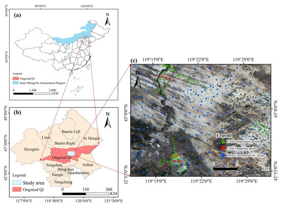
Figure 1.
(a) Location of Ongniud Qi and Inner Mongolia Autonomous Region, China; (b) location of the study area in Ongniud; (c) spatial distribution of selected sampling points. The bottom image is the true color image of Gaofen 5B (blue: 459.7 nm, green: 549.5 nm, red: 660.7 nm).
2.2. Data Sources and Preprocessing
This study utilized Four GF-5B (GaoFen 5B) satellite AHSI (Advanced HyperSpectral Imager) L1-level remote sensing images. GF-5B is the world’s first satellite capable of conducting comprehensive observations of both land and the atmosphere simultaneously. At a swath width of 60 km and a spatial resolution of 30 m, it can capture 330 spectral color channels across the visible light to shortwave infrared (400–2500 nm) spectrum, with a color range nearly nine times wider than that of a typical camera and with nearly 100 times more color channels. Its spectral resolution in the visible spectrum is 5 nanometers. It can effectively detect inland water bodies, terrestrial ecosystems, altered minerals, and rock and mineral types, providing high-quality, highly reliable hyperspectral data for industries such as environmental monitoring, resource exploration, and disaster prevention and mitigation. Table 1 shows the parameters of the GF-5 AHSI camera. For other satellite parameters, please refer to the website (http://114.116.226.59/chinese/satellite/chinese/gf5 (accessed on 19 March 2024)). The experimental data were acquired from 14 September to 5 October 2023, under clear sky conditions with no cloud cover, obtained from the China Natural Resources Satellite Application Center (https://data.cresda.cn/). The preprocessing of the images, including radiometric and atmospheric corrections, was conducted using ENVI 5.3 software.

Table 1.
Key parameters of the GF-5B AHSI camera.
During the processing, certain spectral bands were excluded due to their lower signal-to-noise ratio and other issues. Specifically, water vapor bands (192–203, 246–267, corresponding to 1354–1446 nm and 1808–1985 nm) were removed, along with bands exhibiting poor signal quality (151–154, 314–316, 325–330, corresponding to 1009–1034 nm, 2380–2397 nm, and 2473–2515 nm). In total, 283 spectral bands were retained for further analysis. Compared to the GF-5A satellite data, the GF-5B satellite exhibits a higher signal-to-noise ratio, resolves the defective line issues present in the GF-5A imagery, and reduces striping effects. Consequently, no bad line repair or correction for smile effects was required in this study.
In our study, we have a total of 1962 sample points, including 62 samples collected through field sampling, 800 samples verified through on-site exploration and validation, and 1100 samples interpreted using multi-temporal analysis from Google Earth, Tianditu, and Siwei maps. Fieldwork was conducted in September 2023 and April 2024.
Figure 2 shows the average spectra of seven land cover types on the left and the corresponding field photographs on the right. Among these, the spectra of lush vegetation and salt shell differ significantly from the other five categories, while the remaining five categories exhibit distinct soil spectral characteristics, with visible light and near-infrared reflectance increasing gradually with wavelength. And the reflectance changes are relatively uniform across all bands, with no extreme peaks or troughs. White sand has a significantly higher reflectance than yellow sand in the visible light band, while the differences in other bands are not significant. In overall terms, the reflectance is as follows: salt shell > white sand > yellow sand > bare saline soil > saline soil covered with saline vegetation > sandy soil > lush vegetation.
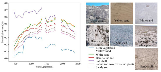
Figure 2.
Spectral curves of different land cover types in the study area and photographs of field sampling points.
3. Methodology
The structure of our study is shown in the flowchart in Figure 3 and consists of the following three main steps: (1) The PSO was used to find the globally optimal decomposition levels, decomposition thresholds, and wavelet basis function for wavelet packet decomposition to remove noise from spectral curves. (2) Four metaheuristic optimization algorithms were applied, including Genetic Algorithm, Bat Algorithm (BA), Differential Evolution (DE), and Particle Swarm Optimization, to extract desertification features and remove spectral redundancies from the original spectra (OS), first-order differential spectra, and continuum-removed spectra (CR). (3) In the comparison of traditional Random Forest models with the ResNet-Transformer model, the most suitable classification model was selected for accurately extracting soil desertification and salinization areas. These approaches aim to advance the precision and efficacy of soil desertification extraction methods, contributing to the sustainable management and utilization of soil resources.
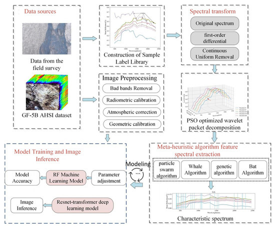
Figure 3.
Methodological flowchart exhibiting the main steps followed in this study.
3.1. Metaheuristic Search Algorithm
In this study, we employ Metaheuristic Search Algorithms to navigate the complex solution space of hyperspectral data analysis, leveraging metaheuristic functions to efficiently guide our search toward optimal solutions. These algorithms utilize pertinent spectral information to intelligently reduce the search space, enhancing the efficiency of the optimization process and accelerating convergence to the optimal solution [35]. It provides an estimation of the quality of the current state to select the most promising search path for the next step [36].
In this research, we employed metaheuristic search algorithms applied in three aspects: (1) Using four metaheuristic algorithms (Genetic Algorithm, Bat Algorithm, Differential Evolution, Particle Swarm Optimization), the feature bands were selected. We compared and analyzed the method that evolved the fastest and achieved the highest global accuracy in selecting hyperspectral feature bands. (2) The Particle Swarm Optimization was utilized to optimize the optimal hyperparameters (maximum depth, node splitting criteria, number of trees of random forests) in land desertification information extraction. (3) Wavelet packet decomposition parameters were optimized by utilizing Particle Swarm Optimization. This optimization method helps determine the optimal decomposition parameters for spectral noise removal.
These applications demonstrated the effectiveness of metaheuristic search algorithms in enhancing the robustness and performance of hyperspectral data processing and modeling tasks. The description of the four metaheuristics we used can be found in the references [37,38,39,40].
The fitness function plays a crucial role in metaheuristic algorithms, guiding the search process by assigning a numerical value to each candidate solution. This enables the algorithm to evolve towards more optimal solutions. In each generation, based on evaluations from the fitness function, the algorithm selects individuals with greater potential for reproduction and evolution, gradually improving the quality of solutions within the population.
In our experiments, we aim to maintain high accuracy while reducing the number of optimal feature bands. We utilized a Cost function as our loss function, which involves calculating the Cost that incorporates both accuracy and the number of feature bands.
The Cost function consists of two components: the error term and the penalty term, where and are the weighting coefficients for the error term and penalty term, respectively. In our experiments, we set the weight coefficient for the error term to 0.8 and the weight coefficient for the penalty term to 0.2. The num_feat and all_feat, respectively, represent the number of selected feature bands and the total number of feature bands.
3.2. PSO Optimizing Globally Optimal Wavelet Packet
Wavelet Packet (WP) decomposition, compared to regular wavelet transforms, decomposes signals into sub-signals of different frequency bands, offering a more flexible decomposition approach. It allows users to select different sub-bands at each decomposition level, thereby better adapting to the signal’s characteristics. However, this flexibility also introduces difficulties in selecting the optimal number of decomposition levels [41]. Moreover, the selection of threshold values at decomposition nodes critically impacts the balance between signal preservation, noise suppression, and smoothness [42]. The wavelet basis function forms the core of wavelet decomposition, determining the frequency resolution and temporal localization characteristics of wavelet packet analysis. Addressing the challenge of determining wavelet packet thresholds, traditional methods often rely on empirical rules or experiments to set threshold parameters. This approach has its limitations: smaller thresholds may allow noise coefficients, while larger thresholds may zero out more coefficients, resulting in image smoothing and potential blurring and artifacts. Incorrect choices of wavelet basis functions and decomposition levels lead to poor adaptability to different signal types and unstable denoising effects. The principles and formulas for wavelet packet noise removal can be found in the reference [26].
To address the issues of selecting the appropriate threshold parameter, wavelet basis function, and decomposition level, the PSO-based optimization method for globally optimal wavelet packet selection is adopted, as illustrated in Figure 4.
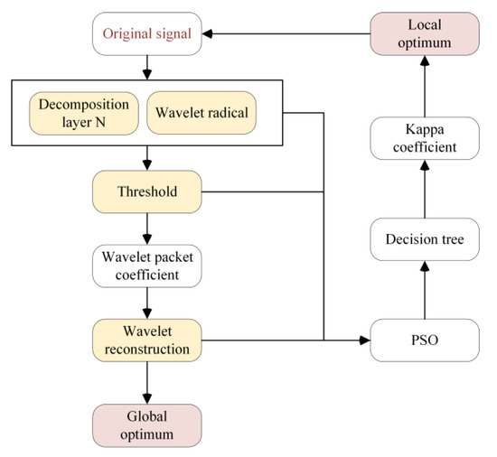
Figure 4.
Flowchart of wavelet packet optimization process using PSO.
During the PSO algorithm iteration process, we iteratively optimize the particle swarm algorithm using wavelet basis functions (bior1.1, bior3.1, coif1, coif2, db3, haar, rbio2.2, sym3, sym2), decomposition layers (1–5 layers), and thresholds (1–200). The denoised sample spectra were obtained by using these optimal parameters to perform wavelet packet decomposition and reconstruction on all sample spectra. Since we did not know the true spectra of pure pixels, we could not accurately calculate the signal-to-noise ratio (SNR) of the reconstructed spectra. Therefore, we used all reconstructed sample spectra, randomly sampling 70% of the samples for input into a decision tree classifier and using the remaining 30% for accuracy evaluation.
Our main steps are outlined as follows:
(1) Each particle performs a decomposition and reconstruction on all spectra, yielding the wavelet packet coefficients for each layer. (2) The wavelet packet coefficients are subjected to threshold processing using a soft thresholding method: components with absolute values below the threshold are set to zero, while those above the threshold are linearly scaled to remove noise while preserving signal features. (3) After thresholding, the processed wavelet packet coefficients are reconstructed to obtain the noise-free signal. (4) In each iteration loop, the local optimal position is updated, ultimately yielding the globally optimal threshold parameters, wavelet basis functions, and decomposition order. Using the optimal threshold parameters, wavelet basis functions, and decomposition order, all sample spectra are subjected to wavelet packet decomposition and reconstruction, yielding the noise-removed sample spectra.
3.3. Modeling Method
3.3.1. PSO Optimization Random Forest Modeling
Random Forest (RF), proposed by Leo Breiman in 2001, enhances overall performance by combining predictions from multiple models. In the Random Forest algorithm, the choice of hyperparameters significantly influences model performance and characteristics. Max_depth controls the maximum depth of the decision trees, while n_estimators dictates the number of trees. A smaller max_depth and fewer trees can prevent overfitting, whereas a larger max_depth and more trees may lead to the more precise fitting of training data but also increase the risk of overfitting. The selection of different criteria affects both model interpretability and accuracy. To optimize these parameters in our experiments, we employed the Particle Swarm Optimization method, like the process used for wavelet packet optimization. The specific steps for optimizing random forest parameters using particle swarm optimization can be found in the reference literature [43]. Specifically, max_depth was searched within the range of 3 to 15, n_estimators within 10 to 50, and criteria included “gini” and “entropy”. Table 2 shows the specific PSO parameter settings for PSO optimization for wavelet packets and random forests. Gini importance is a metric used in random forest models to measure the feature contributions. It quantifies a feature’s impact on classification performance by calculating how much it reduces impurity during decision tree splitting. The higher the value, the more important the feature. In this research, hyperspectral features have high dimensions and significant variation in dimensionality. Gini importance allows for the direct evaluation of features without preprocessing and can effectively identify key bands highly correlated with desertification levels.
Table 2.
Parameter settings for PSO optimization of wavelet packet and random forest.
3.3.2. ResNet-Transformer Modeling
Convolutional Neural network exploding may suffer from gradient exploding. To address these challenges, He et al. introduced Residual Networks (ResNet) in 2015 [31], employing a residual learning framework to optimize the training of deep networks. Central to ResNet is the concept of residual learning. Traditional convolutional networks stack multiple layers, each expected to learn mappings from inputs to outputs. Transformer models were originally introduced in the field of natural language processing (NLP), featuring a core mechanism known as self-attention. This mechanism enables the model to focus on other words in the input sequence when computing the representation of each word, thus capturing long-range dependencies. In the context of hyperspectral image classification, Transformer’s attention mechanism can assist the model in better understanding contextual information within the spectra. Inspired by the Transformer architecture’s impact on NLP, we conceptualize each pixel as serialized information, transforming visual tasks into NLP-like problems. In our network, the ResNet model was applied to capture local patterns and features, while employing Transformer to handle long-range dependencies, thereby harnessing the strengths of both approaches effectively. The network architecture used in this study is illustrated in Figure 5. Table 3 details the specific hyperparameter settings used in the ResNet training.
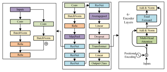
Figure 5.
ResNet-Transformer network structure.
Table 3.
Hyperparameter settings in the training of ResNet-Transformer.
3.4. Evaluation Indicators
- (1)
- Overall accuracy rate:
is the correct sample value and is judged to be the correct value, while is an incorrect sample value that is judged to be the correct value. is a correct sample value but is classified as an incorrect value, while is an incorrect sample value that is judged to be an incorrect value.
- (2)
- The Kappa coefficient is as follows:
is accuracy, and is chance agreement.
- (3)
- Cross-Entropy Loss is as follows:where is the number of samples, is the total number of categories, and is the one-hot encoding model for the true labels, with representing the predicted probability that the i-th sample belongs to the C-th category.
4. Results
4.1. PSO for Wavelet Packet Optimization Process
Spectral preprocessing: Hyperspectral raw image data are often affected by background noise, and there is significant collinearity between similar spectra. To highlight the differences between land cover types, spectral transformations are applied to the original spectral data. Specifically, first-order differentiation (FD) and Continuous Uniform Removal (CR) are performed on both the sample’s original spectrum (OS) and the image spectrum. After the first-order differentiation transformation, spectral regions with sharp variations become more apparent, facilitating the identification of subtle spectral features. The CR transformation, on the other hand, enhances the absorption and reflection characteristics of the spectral curves, emphasizing key spectral features.
Wavelet packet optimization with PSO: Table 4 presents the optimal wavelet packet decomposition parameters obtained through PSO. It should be noted that to expedite the identification of the optimal threshold values and reduce the number of iterations, the OS and CR threshold intervals were set to 0–0.1, while the FD threshold interval was set to 0–20. As shown in Table 4, for the selection of decomposition levels, the optimal levels for the three spectra were found to be four, four, and two, respectively, with none of them reaching the five-level decomposition. Particularly, the CR spectrum chose a two-level decomposition, suggesting that after the removal of the continuum, its frequency structure became simpler compared to the original spectrum. In terms of wavelet base function selection, the optimal wavelet bases for the original and CR spectra were found to be bior3.1, which aligns with numerous studies demonstrating its superiority in signal denoising [44,45]. For the FD spectrum, the optimal wavelet base was selected as sym2, as sym2 has compact support and higher regularity, which means it has better localization properties, making it more efficient for handling FD spectra with significant noise.
Table 4.
The optimal wavelet packet decomposition parameters searched by PSO.
Spectral reconstruction evaluation: Figure 6 compares the transformed and reconstructed spectral curves of the salt–alkali soil based on the optimal PSO decomposition parameters, alongside the original spectra, first-order differential spectra, and continuum-removed spectra. From Figure 6a, it can be seen that the original spectrum (OS) shows minimal change, but effective smoothing has been achieved. Noise around 1000 nm is almost completely removed, and the noise peak around 1724 nm is also reduced. For the first-order differential spectrum (Figure 6b), there are peaks around 1300 nm, 1500 nm, 1724 nm, and 2044. After wavelet packet denoising, the peaks were reduced by half, and the noise oscillation in the 900 nm to 1250 nm range nearly vanished. Due to the discontinuity of the spectrum and the amplification of abnormal data in the differentiation by the first-order differentiation algorithm, wavelet packet noise removal can effectively be suppressed. The CR spectrum (Figure 6c) demonstrates significant noise reduction across all wavelengths while maintaining the general shape of the spectrum and absorption features.
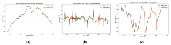
Figure 6.
Comparison of OS, FD, and CR spectra of saline soil before and after wavelet packet denoising. The red line represents the spectra without denoising, while the green line represents the spectra after wavelet packet denoising. (a) Original Spectrum (OS). (b) First-Order Derivative Spectrum (FD). (c) Continuum Removed Spectrum (CR).
4.2. Metaheuristic Algorithm Feature Bands Selection
4.2.1. Optimize Parameter Settings
In the band selection process, four meta-heuristic optimization algorithms, including Genetic Algorithm, Bat Algorithm, Differential Evolution, and Particle Swarm Optimization, were employed to compare their performance in extracting feature bands for land cover classification. These algorithms were applied to feature band selection for three types of spectra: OS, FD, and CR. The parameter settings of the metaheuristic algorithms directly affect the algorithm’s performance, convergence speed, solution quality, and stability. The specific parameter settings for these four optimization methods are shown in Table 5. To ensure a fair comparison of the extraction capabilities, the same particle population size, iteration count, classifier, and fitness loss function were applied to GA, BA, DE, and PSO. Meanwhile, the error term weight coefficient was set to 0.8, and the penalty term weight coefficient was set to 0.2.
Table 5.
Parameter settings for metaheuristic algorithm feature band selection.
4.2.2. Bands Selection Iteration Process
During the early stages of the iteration, the fitness (1-COST) increases rapidly, while in the later stages, it exhibits a stepped rise or tends to plateau. Referring to Equation (1), the reasons for this can be analyzed: in the early iteration stages, the fitness loss function value is mainly influenced by the error rate, which varies due to the different band positions selected. The algorithm focuses on optimizing the positions of the bands that best represent the object features. In the later stages of iteration, the change in the positions of the feature bands becomes smaller, and the algorithm begins to place more emphasis on the influence of the number of bands with smaller weights. As a result, the number of selected feature bands continues to decrease in the later stages.
The results indicate that the ranking of the fitness for selecting bands from the original spectrum by the four metaheuristic algorithms is as follows: GA > DE > BA > PSO for OS, GA > DE > PSO > BA for FD, and DE > GA > BA > PSO for CR.
In terms of iteration fitness, for the OS spectrum, the GA algorithm (Figure 7a) selects 26 bands, achieving a fitness of 0.978. The iteration process is relatively stable and does not converge to a local optimum, making it the optimal feature band selection algorithm for the OS spectrum. For the FD spectrum (Figure 7b), the GA algorithm is also the optimal band selection method, but it selects 45 bands. This is likely due to the increased spectral details after the FD transformation, requiring more feature bands to represent the data. For the CR spectrum (Figure 7c,f,i,l), the fitness decreases significantly compared to OS and FD. Regardless of the algorithm, a larger number of bands is selected, with DE selecting the fewest 48 bands, but the fitness only reaches 0.946. The BA and PSO algorithms exhibit poor performance in reducing the number of selected bands during the later stages of optimization, with the final number of selected bands exceeding 100 in most cases. Although the fitness increases rapidly in the early stages of iteration, it shows minimal change in the later stages, failing to escape from a local optimum. This suggests that metaheuristic algorithms based on evolutionary theory are more suitable for finding the optimal or near-optimal solutions for feature band selection compared to population-based metaheuristic algorithms, as they are less prone to getting stuck in local optima.
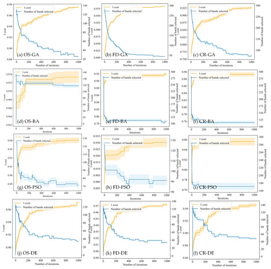
Figure 7.
The iteration process of the GA, BA, PSO, and DE algorithms applied to the OS, FD, and CR spectra. The orange line represents the fitness (1-Cost) curve, while the blue line shows the change in the number of selected bands.
4.2.3. Bands and Runtime
Figure 8 illustrates the final number of selected bands and the corresponding running times for the OS, FD, and CR spectra after applying the GA, BA, PSO, and DE algorithms. The results indicate that the four metaheuristic algorithms prioritize optimization speed in the following order: BA > DE > GA > PSO. Notably, although the BA algorithm does not achieve the optimal positions compared to GA and selects more feature bands, its pulse intensity and emission frequency update mechanisms contribute to the algorithm’s ability to adaptively adjust its search range and speed during the optimization process. As a result, BA achieves faster optimization, reaching 1000 iterations in roughly half the time used by other algorithms. For the three spectral types, the ranking of computational speed for feature band selection is as follows: OS > FD > CR. This ranking aligns with the trend in the number of selected bands. As the number of selected feature bands increases, the number of individuals (candidate solutions) involved in the algorithm’s calculations also grows. Consequently, the algorithm needs to search for the optimal solution in a larger search space. More features mean that more computations are required during each iteration, including fitness function evaluation and individual update operations.
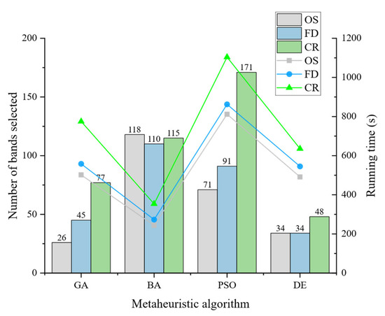
Figure 8.
The final number of selected bands and runtimes for OS, FD, and CR spectra using GA, BA, PSO, and DE algorithms are depicted in the graph. The bar chart represents the number of bands selected by each algorithm, using the left axis. The line plot represents the runtime of each algorithm, using the right axis.
4.2.4. Feature Bands Selected
Figure 9 is a schematic diagram showing the locations of the selected characteristic bands and the averaged spectral curves of the land cover for the GA and DE algorithms applied to the OS, FD, and CR spectra. In the figure, for the original spectrum (Figure 9a), both GA and DE selected a large number of bands in the 380–780 nm visible light range. Among these, 46.2% of the visible light bands selected by GA account for the total number of bands, while 66.7% of the visible light bands selected by DE account for the total number of bands. This is because land covers such as vegetation, saline areas, sandy land, and salt crusts exhibit different colors and brightness in the visible light range, making it easier to distinguish them [46]. Additionally, many shortwave infrared bands in the 1950–2300 nm range were also selected. This is similar to the findings of Chapman [47], who used shortwave infrared bands for salt flat identification, and Drake [48], who studied salt absorption peaks in evaporative minerals using SWIR bands, indicating that shortwave infrared bands are characteristic for identifying saline and alkaline areas.
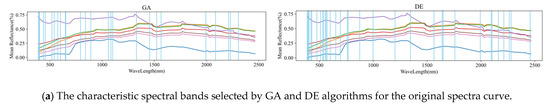
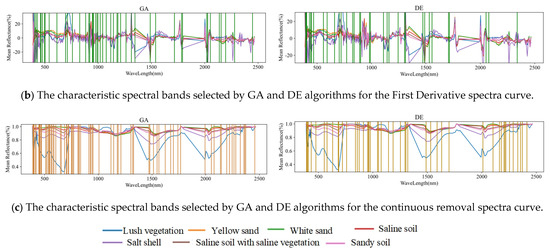
Figure 9.
The feature bands selected by the GA and DE algorithms for the OS, FD, and CR spectral curves. Different colored lines correspond to the mean spectral signatures.
For the FD spectrum (Figure 9b), many spectral bands were selected, with bands distributed across various intervals. This is because FD focuses not on the absorption depth of land cover features but on the shape of the absorption characteristics. Moreover, after first-order differentiation, more peaks appeared in the spectrum, enhancing the high-frequency components of the data. First-order differentiated spectra are better at eliminating the influence of soil matrix background and reducing the scattering effects caused by particle size, making the model more focused on the subtle spectral information generated by trace components.
For the CR spectrum (Figure 9c), the specific locations of the selected bands differed between the two algorithms, but the distribution across the intervals was generally consistent. While some valid features were identified, the curve became very smooth, and small peaks were missing. Therefore, although the CR transformation selected more bands, its fitness remained relatively low.
4.2.5. Bands’ Importance
Based on the analysis of the results in Figure 9, the optimal feature selection algorithm for the OS and FD is the GA, while for the CR spectrum, the optimal feature selection algorithm is the DE algorithm. The feature bands selected by the optimal feature selection algorithms for the three spectra were evaluated based on the Gini importance score in Random Forest to measure their contribution to the prediction results. In different spectral transformations, features may be either amplified or compressed, leading to changes in the selected feature band locations and their importance. For the OS spectrum features (Figure 10a), the top six most important bands are in the visible range, accounting for 41.9% of the total importance, followed by six shortwave infrared bands, which contribute 27.7% to the total importance. The three selected near-infrared bands account for only 4.7%, consistent with the previous analysis. For the first-order differential spectrum (Figure 10b), the selected 1488.75 nm band accounts for 9.4% of the total importance, and the 2145.25 nm band accounts for 5%. As shown in Figure 9 of the mean spectral curves for land covers, these two bands exhibit distinct separation boundaries for the six land cover types, which are not apparent in the original spectrum. For the CR-transformed spectrum (Figure 10c), the most important feature is also the 395.6 nm band, with other important bands concentrated around the absorption or reflection peak regions.
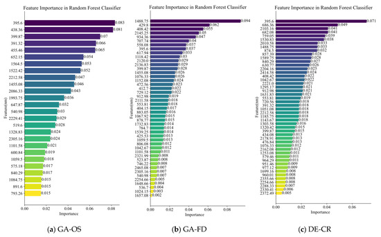
Figure 10.
The characteristic spectral bands selected by the respective feature selection algorithms (GA for OS and FD spectra; DE for CR spectra), and their importance in the random forest classifier.
4.3. Desertification (Sand and Saline Soil) Information Extraction Based on the ResNet-Transformer Model
4.3.1. Model Evaluation
To evaluate the performance of the ResNet-Transformer model, we compared it with the Random Forest model. In the Random Forest model, we also applied the PSO algorithm to optimize the maximum depth, tree depth, and node splitting criteria of the decision trees. The results showed that the optimal hyperparameters were: a maximum depth of 10, entropy as the best node splitting criterion, and the use of 28 base learners (decision trees). We conducted combination experiments using both the ResNet-Transformer model and the Random Forest model, with three spectral transformations (original, first-order derivative, and continuum removal), noise removal using wavelet packet transform, and feature extraction algorithms, respectively. The same dataset was split into training and validation data, and a 10-fold cross-validation method was used to evaluate the classification performance. The overall accuracy is shown in Table 6.
Table 6.
Comparison of modeling validation accuracy for desertification information extraction using different algorithms.
From the results shown in Table 6, the ResNet-Transformer model significantly outperforms the traditional RF model, particularly in modeling raw spectral curves without wavelet packet transformation or feature extraction, where it achieves a 3.23% higher validation accuracy than RF. Among all combined methods, the WP-GA-FD-ResNet-Transformer approach—incorporating first-order derivative (FD) transformation, wavelet packet denoising (WP), and genetic algorithm (GA) feature selection—delivers the highest accuracy, with a Kappa coefficient of 0.9746 and validation accuracy of 97.82%. The accuracy ranking across different spectral transformations follows FD > OS > CR. Although the cost loss values between FD and OS during feature extraction were comparable, their validation accuracy differed by 1–3%, likely because FD selected more spectral bands to represent ground features, increasing the weight of band quantity and consequently raising the cost. Consistent with previous findings, CR-transformed data still underperformed compared to the raw spectra. Furthermore, both WP denoising and the GA algorithm played crucial roles in improving modeling accuracy: with the raw spectra, WP denoising alone increased validation accuracy by 1.7% in the RF classifier, while GA-based feature selection alone improved it by 1.4%.
4.3.2. Loss in Training and Validation Sets
Figure 11 shows the changes in training and validation loss during the training process of the WP-GA-FD-ResNet-Transformer model. From the figure, it can be observed that during the early stages of training, due to the high initial learning rate, the training and validation losses decrease rapidly. However, as training progresses to approximately 100 iterations, both the training and validation losses begin to stabilize around 0.15. As the number of iterations increases, the losses for both the training and validation sets level off, and they become very close to each other. This indicates that the ResNet-Transformer model effectively avoids overfitting.
Figure 11.
Variation in the loss in training and validation sets with the increasing number of iterations in the ResNet-Transformer model.
4.3.3. Confusion Matrix
Figure 12 shows a comparative analysis of the FD-ResNet-Transformer and FD-RF models after wavelet packet noise removal and GA-based feature band selection. From the results, it can be observed that both models perform well in identifying land covers with significant spectral differences, such as dense vegetation, yellow sand, salt crust, and sandy soil, with minimal confusion with other land covers. However, when dealing with land covers that have small spectral differences, such as white sand, saline–alkali soil, and saline–alkali soil covered with saline vegetation, the ResNet-Transformer model maintains better performance, whereas the traditional RF model tends to experience confusion. Only 90.28% prediction accuracy was achieved for features like saline soil, while 95.5% prediction accuracy was achieved for the ResNet-Transformer. This may be because the ResNet-Transformer network, when extracting features from land covers with small spectral differences, leverages the convolutional structure to capture local information and the Transformer’s self-attention mechanism to establish long-range dependencies, thereby capturing both spectral shape features and subtle spectral differences.
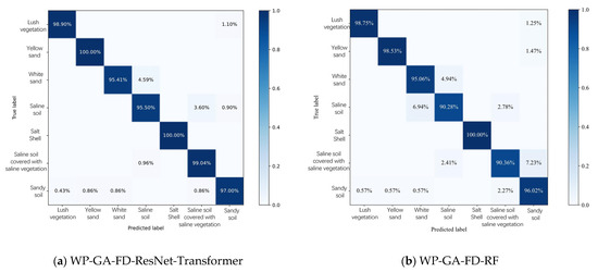
Figure 12.
Confusion matrix for the WP-GA-FD-ResNet-Transformer and WP-GA-FD-RF models.
4.3.4. Extraction in Land Desertification Areas
Figure 13 shows the distribution maps of sandification and salinization areas extracted using the WP-GA-FD-ResNet-Transformer and FD-RF models in the experimental area. From the results, both models perform well in identifying the easily distinguishable salt crust. However, the WP-GA-FD-ResNet-Transformer model produces more compact pixel clusters for yellow sand and saline soil, whereas the WP-GA-FD-RF model results in more fragmented clusters, leading to misclassifications of the transition areas between white sand and vegetation as saline–alkali soil. In Area A, the WP-GA-FD-ResNet-Transformer model more accurately reflects the real surface cover distribution of yellow sand and white sand, while the FD-RF model misidentifies many fewer distinct yellow sand areas as white sand.
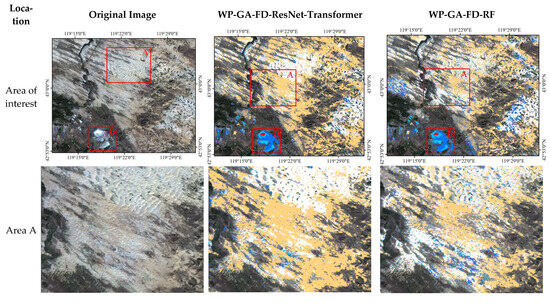
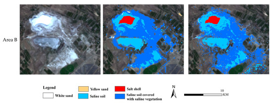
Figure 13.
Comparison of extracted images using the WP-GA-FD-Resnet Transformer and the WP-GA-FD-RF for areas A and B.
After the model was constructed, image inference was performed on four images to obtain the distribution of desertification and saline soil (Figure 14). The distribution area of each type of land feature was calculated geometrically in ArcMap. The area of yellow sand in Ongniud Qi is approximately 736.7 square kilometers, and the white sand area is about 245 square kilometers. According to the National Ecological Status Survey and Evaluation Technical Standards [49], the yellow sand and white sand in this region are classified as severely or extremely severely desertified areas, while the remaining soils in the region are classified as lightly or moderately sandy soils. Overall, Ongniud Qi exhibits a serious degree of sandification, being the area with the largest distribution of sand and the most severe sandification in Chifeng. In the western and southwestern regions of Ongniud Qi, the sandification is relatively mild, while the central, eastern, and northern regions show more severe sandification, especially along the banks of the Shaolang River, where large patches of sand are present. However, it is noteworthy that during field investigations, it was found that the local government is actively implementing various measures to combat wind erosion and sand fixation. These measures include dividing the sandy areas into “grid-like” sections, using roads for sand control, constructing shelterbelts that combine trees, shrubs, and grasses, and building sand barriers using materials such as firewood, straw, crop stalks, branches, and clay to reduce the amount of sand transported by wind and decrease wind speeds between the barriers, thereby promoting sand recovery.
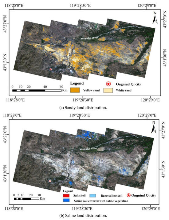
Figure 14.
Predicted distribution of sandy and saline land in Ongniud Qi.
Based on the statistical results from Figure 14 on the distribution of saline land, the total area of saline land in Ongniud Qi is approximately 128.25 square kilometers, including 0.48 square kilometers of salt crust, 5.83 square kilometers of exposed saline–alkali land, and 121.94 square kilometers of saline land covered with saline plants. Saline soil is mainly distributed around seasonal lakes, rivers, and some low-lying areas. For example, the seasonal lake Qigan Noer in Wudan Town, located in the Qigan Dapaozi area, experiences increased precipitation in the summer. Due to the surrounding higher terrain, water-soluble salts are carried by water from higher elevations to lower areas. After the rainy season, the dissolved salts accumulate on the surface of the soil once the moisture evaporates. At the Qigan Dapaozi lake, the surface vegetation changes progressively from saline–alkali land covered by saline plants to exposed saline–alkali land, and finally to large patches of exposed salt crust as one moves toward the center of the lake. The degree of salinization increases as one move inward toward the center. Samples collected from the low-lying area at the center of the lake were analyzed using the X-ray diffraction (XRD) of minerals. The results showed that the salt content of halite (rock salt) was 32%, with the contents of water-soluble salts and natural soda ash at 8% and 14%, respectively.
5. Discussion
5.1. Limitations of PSO-Optimized Wavelet Packet
The true spectral characteristics of objects are influenced by factors such as sensor resolution and soil heterogeneity and by significant differences between laboratory measured spectra and satellite data, making the “pure spectrum” merely a theoretical concept in remote sensing data. In practical applications, it is difficult to determine the actual pure spectrum of objects, so it is not possible to use a quantitative metric to evaluate the effectiveness of the reconstructed curves after decomposition. For each curve, it is difficult to find a specific quantifiable fitness function. Therefore, when using PSO for wavelet packet decomposition, we employ the modeling classification accuracy to assess the decomposition effect. Additionally, all spectral curves use the same threshold, wavelet packet decomposition layer number, and wavelet basis function. However, each spectral curve should have optimal decomposition parameters. Although differences may be minimal within the same category, spectral signals still exhibit significant variations under different soil types and environmental conditions, resulting in substantial differences in high-frequency noise performance. Therefore, in future studies on adaptive algorithm-based wavelet packet noise removal, supplementary metrics such as F1-score, information, redundancy, and separability of target background should be considered to expand the objective function in multiple dimensions. Simultaneously, clustering should be used to generate parameter groups, such as desertified soil groups and saline soil groups, with decomposition parameters optimized independently for each group.
5.2. Uncertainty in Feature Selection Bands
During the feature selection process, we used the overall modeling accuracy of all classified categories in the region as the criterion. Therefore, the selected bands were chosen to maximize the distinction among all classified categories. These bands can only represent the optimal ones for distinguishing the overall classified land cover types. Due to the influence of mixed pixels, the spectral characteristics of vegetation and clay, which are typically distinct, appear relatively weak here. Additionally, the selected bands sensitive to the features of saline land and sandy soil are subject to significant interference. In future research, we will balance overall classification accuracy and specific feature sensitivity, increase hierarchical feature importance assessment, and conduct pixel purity screening at the same time. We will use the PPI (pixel purity index) to identify pure pixels in the research area, and perform feature selection based solely on the spectral data of pure pixels. We will also perform spatial heterogeneity correction, in which pixels in highly heterogeneous regions are removed using moving window statistics (e.g., spectral standard deviation within a 3 × 3 window) to reduce the interference of mixed pixels on band sensitivity.
5.3. Confusion Between Saline and White Sands
Many studies have shown that factors such as salt type, soil mineralogy, moisture content, organic matter content, color and brightness, roughness, and vegetation coverage significantly influence the spectra of soils. However, when only visible and near-infrared wavelengths are considered, soil salinity levels have a limited impact on the spectral response within this range. In particular, white sand and saline–alkali soils exhibit a high degree of spectral similarity in the visible wavelength range [50]. To investigate the reasons for the confusion between saline soils (with withered vegetation) and white sand (with withered vegetation), we employed t-distributed stochastic neighbor embedding (t-SNE) to calculate the similarity between each pair of points in the high-dimensional data. The visualization of sample spectra in high-dimensional space was mapped to two dimensions, as shown in the t-SNE plot (Figure 15), where the four sample types overlap, indicating high spectral similarity and making them prone to confusion during modeling and identification. As illustrated in Figure 16, in the transition zone between white sand and vegetation, small natural water depressions often form along the edges of sand dunes during rainfall. The fine minerals weathered in the sand accumulate and clayify under the action of water flow. Consequently, the complexity of the accumulated components and the texture in this region creates difficulties in spectral extraction.
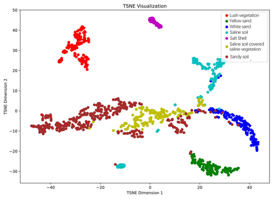
Figure 15.
Two-dimensional t-SNE visualization of sample spectra.
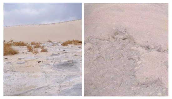
Figure 16.
Land salinization in dune basins.
6. Conclusions
This study utilized GF-5 AHSI data to propose a set of methods for extracting land desertification. The particle swarm optimization algorithm was used to optimize the wavelet packet decomposition parameters, automatically selecting the optimal noise removal parameters. Based on the objective function involving the number of constructed bands and the Kappa coefficient, the spectral feature extraction capabilities of four metaheuristic algorithms for OS, FD, and CR spectra were compared. To address the limitation of traditional machine learning methods in capturing global information, a ResNet-Transformer model was constructed to extract desertification areas. This study draws the following conclusions:
(1) The particle swarm optimization algorithm could automatically identify the global optimal parameters for wavelet decomposition and reconstruction, effectively removing high-frequency noise from the spectrum while preserving essential spectral information.
(2) For OS and FD spectra, the genetic algorithm was the optimal feature selection algorithm. Using only feature selection based on the GA algorithm could improve the validation accuracy of the OS spectrum in the random forest classifier by 1.4%. In addition to visible light, attention should be paid to the role of shortwave infrared radiation in land desertification extraction.
(3) Among all models, the WP-GA-FD-ResNet-Transformer model, which combines wavelet packet denoising (WP), genetic algorithm feature selection (GA-FD), and the ResNet-Transformer hybrid network, achieved the highest accuracy in soil sandification and salinization extraction, and was closer to the true land cover distribution. This indicated that the newly constructed model captures spectral shape features while also considering subtle spectral differences.
This study proposes a reference solution for hyperspectral land desertification identification in terms of noise removal, band selection, and model construction. For future hyperspectral noise removal, multiple indicators can be added as objective functions for adaptive wavelet packet parameter selection strategies, and different optimization algorithms can be integrated to enhance model generalization.
Author Contributions
Conceptualization, R.L.; data curation, Y.T. and Q.Z.; formal analysis, W.L.; investigation, W.L. and Y.D.; methodology, F.G. and P.Z.; project administration, R.L.; resources, R.L.; software, W.L.; supervision, R.L.; validation, W.L. and Y.L.; visualization, W.L.; writing—review and editing, J.X., R.L., and T.Z. All authors have read and agreed to the published version of the manuscript.
Funding
This study was funded by National Natural Science Foundation of China, grant numbers 42271408, 41701434.
Data Availability Statement
The data that support the findings of this study are available from the corresponding author upon reasonable request.
Conflicts of Interest
The authors declare that they have no known competing financial interests or personal relationships that could have appeared to influence the work reported in this paper.
References
- Verstraete, M.M. Defining desertification: A review. Clim. Change 1986, 9, 5–18. [Google Scholar] [CrossRef]
- Xie, J.; Lu, Z.; Feng, K. Effects of Climate Change and Human Activities on Aeolian Desertification Reversal in Mu Us Sandy Land, China. Sustainability 2022, 14, 1669. [Google Scholar] [CrossRef]
- Dregne, H.; Kassas, M.; Rozanov, B. A new assessment of the world status of desertification. Desertif. Control. Bull. 1991, 20, 7–18. [Google Scholar]
- Hulme, M.; Kelly, M. Exploring the links between desertification and climate change. Environ. Sci. Policy Sustain. Dev. 1993, 35, 4–45. [Google Scholar] [CrossRef]
- Su, Y.Z.; Zhao, W.Z.; Su, P.X.; Zhang, Z.H.; Wang, T.; Ram, R. Ecological effects of desertification control and desertified land reclamation in an oasis–desert ecotone in an arid region: A case study in Hexi Corridor, northwest China. Ecol. Eng. 2007, 29, 117–124. [Google Scholar] [CrossRef]
- Zhang, Z.; Huisingh, D. Combating desertification in China: Monitoring, control, management and revegetation. J. Clean. Prod. 2018, 182, 765–775. [Google Scholar] [CrossRef]
- Cai, J.; Yu, W.; Fang, Q.; Zi, R.; Fang, F.; Zhao, L. Extraction of Rocky Desertification Information in the Karst Area Based on the Red-NIR-SWIR Spectral Feature Space. Remote Sens. 2023, 15, 3056. [Google Scholar] [CrossRef]
- Gao, L.; Wang, D.; Zhuang, L.; Sun, X.; Huang, M.; Plaza, A. BS 3 LNet: A new blind-spot self-supervised learning network for hyperspectral anomaly detection. IEEE Trans. Geosci. Remote Sens. 2023, 61, 1–18. [Google Scholar]
- West, H.; Quinn, N.; Horswell, M. Remote sensing for drought monitoring & impact assessment: Progress, past challenges and future opportunities. Remote Sens. Environ. 2019, 232, 111291. [Google Scholar]
- Chen, L.; Tan, K.; Wang, X.; Chen, Y. A rapid soil Chromium pollution detection method based on hyperspectral remote sensing data. International J. Appl. Earth Obs. Geoinf. 2024, 128, 103759. [Google Scholar] [CrossRef]
- Feng, Q.; Ma, H.; Jiang, X.; Wang, X.; Cao, S. What has caused desertification in China? Sci. Rep. 2015, 5, 15998. [Google Scholar] [CrossRef] [PubMed]
- Huang, S.; Tang, L.; Hupy, J.P.; Wang, Y.; Shao, G. A commentary review on the use of normalized difference vegetation index (NDVI) in the era of popular remote sensing. J. For. Res. 2021, 32, 1–6. [Google Scholar] [CrossRef]
- Qi, J.; Chehbouni, A.; Huete, A.R.; Kerr, Y.H.; Sorooshian, S. A modified soil adjusted vegetation index. Remote Sens. Environ. 1994, 48, 119–126. [Google Scholar] [CrossRef]
- Bannari, A.; Morin, D.; Bonn, F.; Huete, A. A review of vegetation indices. Remote Sens. Rev. 1995, 13, 95–120. [Google Scholar] [CrossRef]
- Jiang, Z.; Huete, A.R.; Chen, J.; Chen, Y.; Li, J.; Yan, G.; Zhang, X. Analysis of NDVI and scaled difference vegetation index retrievals of vegetation fraction. Remote Sens. Environ. 2006, 101, 366–378. [Google Scholar] [CrossRef]
- Ma, H.W.; Wang, Y.F.; Guo, E.L. Remote sensing monitoring of aeolian desertification in Ongniud Banner based on GEE. Arid. Zone Res. 2023, 40, 504–516. [Google Scholar]
- Guo, B.; Ye, W. An Optimal Monitoring Model of Desertification in Naiman Banner Based on Feature Space Utilizing Landsat8 OLI Image. IEEE Access 2020, 8, 4761–4768. [Google Scholar] [CrossRef]
- Liu, Y.; Ci, L. The evaluating indicator system of grass land desertification in Mu US sandy land. J. Desert Res. 1998, 18, 366–371. [Google Scholar]
- Chen, H.; Ma, Y.; Zhu, A.; Wang, Z.; Zhao, G.; Wei, Y. Soil salinity inversion based on differentiated fusion of satellite image and ground spectra. International J. Appl. Earth Obs. Geoinf. 2021, 101, 102360. [Google Scholar] [CrossRef]
- Uddin, M.P.; Mamun, M.A.; Hossain, M.A. PCA-based feature reduction for hyperspectral remote sensing image classification. IETE Tech. Rev. 2021, 38, 377–396. [Google Scholar] [CrossRef]
- Lavanya, K.; Obaid, J.A.; Sumaiya Thaseen, I.; Abhishek, K.; Saboo, K.; Paturkar, R. Terrain mapping of LandSat8 images using MNF and classifying soil properties using ensemble modelling. Int. J. Nonlinear Anal. Appl. 2020, 11, 527–541. [Google Scholar]
- Sadeghian, Z.; Akbari, E.; Nematzadeh, H.; Motameni, H. A review of feature selection methods based on meta-heuristic algorithms. J. Exp. Theor. Artif. Intell. 2023, 37, 1–51. [Google Scholar] [CrossRef]
- Zhao, H.; Bruzzone, L.; Guan, R.; Zhou, F.; Yang, C. Spectral-spatial genetic algorithm-based unsupervised band selection for hyperspectral image classification. IEEE Trans. Geosci. Remote Sens. 2021, 59, 9616–9632. [Google Scholar] [CrossRef]
- Sun, X.; Lin, P.; Shang, X.; Pang, H.; Fu, X. MOBS-TD: Multi-objective band selection with ideal solution optimization strategy for hyperspectral target detection. IEEE J. Sel. Top. Appl. Earth Obs. Remote Sens. 2024, 17, 10032–10050. [Google Scholar] [CrossRef]
- Ou, X.; Wu, M.; Tu, B.; Zhang, G.; Li, W. Multi-objective unsupervised band selection method for hyperspectral images classification. IEEE Trans. Image Process. 2023, 32, 1952–1965. [Google Scholar] [CrossRef]
- Liu, W.; Huo, H.; Zhou, P.; Li, M.; Wang, Y. Research on Hyperspectral Modeling of Total Iron Content in Soil Applying LSSVR and CNN Based on Shannon Entropy Wavelet Packet Transform. Remote Sens. 2023, 15, 4681. [Google Scholar] [CrossRef]
- Bhandari, A.K.; Kumar, A.; Singh, G.K.; Soni, V. Performance study of evolutionary algorithm for different wavelet filters for satellite image denoising using sub-band adaptive threshold. J. Exp. Theor. Artif. Intell. 2016, 28, 71–95. [Google Scholar] [CrossRef]
- Ge, G.; Shi, Z.; Zhu, Y.; Yang, X.; Hao, Y. Land use/cover classification in an arid desert-oasis mosaic landscape of China using remote sensed imagery: Performance assessment of four machine learning algorithms. Glob. Ecol. Conserv. 2020, 22, e00971. [Google Scholar] [CrossRef]
- Li, P.; Chen, P.; Shen, J.; Deng, W.; Kang, X.; Wang, G.; Zhou, S. Dynamic Monitoring of Desertification in Ningdong Based on Landsat Images and Machine Learning. Sustainability 2022, 14, 7470. [Google Scholar] [CrossRef]
- Aldabbagh, Y.A.N.; Shafri, H.Z.M.; Mansor, S.; Ismail, M.H. Desertification prediction with an integrated 3D convolutional neural network and cellular automata in Al-Muthanna, Iraq. Environ. Monit. Assess. 2022, 94, 715. [Google Scholar] [CrossRef]
- He, K.; Zhang, X.; Ren, S.; Sun, J. Deep residual learning for image recognition. In Proceedings of the IEEE Conference on Computer Vision and Pattern Recognition, Las Vegas, NV, USA, 27–30 June 2016; pp. 770–778. [Google Scholar]
- Wang, W.; Jiang, Y.; Wang, G.; Guo, F.; Li, Z.; Liu, B. Multi-Scale LBP Texture Feature Learning Network for Remote Sensing Interpretation of Land Desertification. Remote Sens. 2022, 14, 3486. [Google Scholar] [CrossRef]
- Jaderberg, M.; Simonyan, K.; Zisserman, A. Spatial transformer networks. Adv. Neural Inf. Process. Syst. 2015, 2, 2017–2025. [Google Scholar]
- Jiang, H.; Wu, R.; Zhang, Y.; Li, M.; Lian, H.; Fan, Y.; Yang, W.; Zhou, P. Classification Model of Grassland Desertification Based on Deep Learning. Sustainability 2024, 16, 8307. [Google Scholar] [CrossRef]
- Du, K.L.; Swamy, M.N.S. Search and Optimization by Metaheuristics. Techniques and Algorithms Inspired by Nature; Springer Nature: Berlin/Heidelberg, Germany, 2016; pp. 1–10. [Google Scholar]
- Abdel-Basset, M.; Abdel-Fatah, L.; Sangaiah, A.K. Metaheuristic algorithms: A comprehensive review. Computational Intelligence for Multimedia Big Data on the Cloud with Engineering Applications; Elsevier: Amsterdam, The Netherlands, 2018; pp. 185–231. [Google Scholar]
- Haldurai, L.; Madhubala, T.; Rajalakshmi, R. A study on genetic algorithm and its applications. Int. J. Comput. Sci. Eng. 2016, 4, 139–143. [Google Scholar]
- Yang, X.S.; Hossein Gandomi, A. Bat algorithm: A novel approach for global engineering optimization. Eng. Comput. 2012, 29, 464–483. [Google Scholar] [CrossRef]
- Mayer, D.G.; Kinghorn, B.P.; Archer, A.A. Differential evolution—An easy and efficient evolutionary algorithm for model optimisation. Agric. Syst. 2005, 83, 315–328. [Google Scholar] [CrossRef]
- Schutte, J.F.; Reinbolt, J.A.; Fregly, B.J.; Haftka, R.T.; George, A.D. Parallel global optimization with the particle swarm algorithm. Int. J. Numer. Methods Eng. 2004, 61, 2296–2315. [Google Scholar] [CrossRef]
- Hosseini, H.; Syed-Yusof, S.K.B.; Fisal, N.; Farzamnia, A. Compressed wavelet packet-based spectrum sensing with adaptive thresholding for cognitive radio. Can. J. Electr. Comput. Eng. 2015, 38, 31–36. [Google Scholar] [CrossRef]
- Mingliang, L.; Keqi, W.; Laijun, S.; Jianfeng, Z. A new fault diagnosis method for high voltage circuit breakers based on wavelet packet and radical basis function neural network. Open Cybern. Syst. J. 2014, 8, 410–417. [Google Scholar]
- Liu, D.; Sun, K. Random forest solar power forecast based on classification optimization. Energy 2019, 187, 115940. [Google Scholar] [CrossRef]
- Das, O.; Bagci Das, D. Smart machine fault diagnostics based on fault specified discrete wavelet transform. J. Braz. Soc. Mech. Sci. Eng. 2023, 45, 55. [Google Scholar] [CrossRef]
- Yousef, A.N.; Behzad, T.; Abolghasem, K.R.; Shahram, S.; Kaveh, K.; Amin, J. A combined Parzen-wavelet approach for detection of vuggy zones in fractured carbonate reservoirs using petrophysical logs. J. Pet. Sci. Eng. 2014, 119, 1–7. [Google Scholar] [CrossRef]
- Bannari, A.; El-Battay, A.; Bannari, R.; Rhinane, H. Sentinel-MSI VNIR and SWIR Bands Sensitivity Analysis for Soil Salinity Discrimination in an Arid Landscape. Remote Sens. 2018, 10, 855. [Google Scholar] [CrossRef]
- Chapman, J.E.; Rothery, D.A.; Francis, P.W.; Pontual, A. Remote sensing of evaporite mineral zonation in salt flats (salars). Remote Sens. 1989, 10, 245–255. [Google Scholar] [CrossRef]
- Drake, N.A. Reflectance spectra of evaporite minerals (400–2500 nm): Applications for remote sensing. Int. J. Remote Sens. 1995, 16, 2555–2571. [Google Scholar] [CrossRef]
- GB/T 24255-2009; Technical Specifications for Monitoring Desertified Land. Standards Press of China: Beijing, China, 2009.
- Verma, K.S.; Saxena, R.K.; Barthwal, A.K.; Deshmukh, S.N. Remote sensing technique for mapping salt affected soils. Int. J. Remote Sens. 1994, 15, 1901–1914. [Google Scholar] [CrossRef]
Disclaimer/Publisher’s Note: The statements, opinions and data contained in all publications are solely those of the individual author(s) and contributor(s) and not of MDPI and/or the editor(s). MDPI and/or the editor(s) disclaim responsibility for any injury to people or property resulting from any ideas, methods, instructions or products referred to in the content. |
© 2025 by the authors. Licensee MDPI, Basel, Switzerland. This article is an open access article distributed under the terms and conditions of the Creative Commons Attribution (CC BY) license (https://creativecommons.org/licenses/by/4.0/).