Impact of Input Image Resolution on Deep Learning Performance for Side-Scan Sonar Classification: An Accuracy–Efficiency Analysis

Abstract

Side-scan sonar (SSS) image classification is crucial for underwater applications, but the trade-off between the accuracy afforded by high-resolution images and the associated computational cost challenges deployment, particularly on resource-constrained platforms like AUVs. This study systematically investigates and quantifies this accuracy–efficiency trade-off in SSS image classification by varying input resolution. Using two distinct SSS datasets and a resolution-adaptive deep learning strategy employing MobileNetV2 and ResNet variants across six resolutions, we evaluated classification accuracy and computational metrics. Results demonstrate a clear inverse relationship: decreasing resolution significantly reduces computational load and processing times but lowers classification accuracy, with the degradation being more pronounced for the more complex four-class dataset. Notably, model test accuracy did not necessarily increase monotonically with resolution. Importantly, acceptable accuracy levels above 90% or 80% could be maintained at significantly lower resolutions, offering substantial efficiency gains. In conclusion, strategically reducing SSS image resolution based on application-specific accuracy requirements is a viable approach for optimizing computational resources. This work provides a quantitative framework for navigating this trade-off and underscores the need for developing SSS-specific architectures for future advancements.

1. Introduction

Side-scan sonar (SSS) stands as a cornerstone technology in underwater remote sensing, delivering high-resolution acoustic imagery of the seabed irrespective of water turbidity. Its capability to rapidly survey large areas makes it indispensable for a wide array of marine applications. These include detailed seabed mapping, comprehensive geological surveys [1], marine archeological investigations, critical infrastructure monitoring like pipeline inspections [2], benthic habitat characterization, and the detection of various underwater objects such as shipwrecks, submerged obstacles, and potential geohazards [3]. However, the sheer volume of data generated by SSS systems presents a significant challenge for manual analysis, which is not only labor-intensive and time-consuming but also demands considerable expertise and can suffer from inconsistencies [2,3,4]. To address these challenges, the application of deep learning (DL), especially Convolutional Neural Networks (CNNs), has become increasingly prominent, offering new capabilities for automated analysis. Mirroring their success in other image analysis domains [4,5,6], CNNs have demonstrated remarkable efficacy in automating the interpretation of SSS imagery. They have yielded significant performance improvements in diverse tasks, including seabed sediment classification [7], underwater object detection [3,8,9,10], and semantic segmentation of sonar mosaics [1,11], frequently surpassing the capabilities of traditional image processing techniques. Furthermore, methodologies like transfer learning have enabled leveraging knowledge from models pre-trained on extensive optical image datasets, further enhancing classification accuracy in the SSS domain [2,12].

Despite these advances, a critical challenge remains: the high computational demands of advanced CNN models limit their use for SSS image analysis, particularly on resource-constrained platforms like Autonomous Underwater Vehicles (AUVs) [7,13]. This challenge is fundamentally rooted in two interconnected factors. First, the inherent characteristics of SSS imagery—such as speckle noise, intensity variations, and complex seabed textures—often necessitate deeper and more complex network designs for robust feature extraction [14]. Second, the pursuit of higher accuracy often involves using high-resolution images, which concurrently escalates the computational burden of processing power, memory, and energy exponentially [15]. AUVs serve as pivotal platforms for autonomous marine exploration and monitoring, yet they typically operate under strict limitations regarding onboard computational capacity (often lacking powerful GPUs), available power budgets, and data transmission bandwidth. The substantial computational expense associated with processing high-resolution SSS data directly onboard frequently prohibits real-time analysis and adaptive decision-making, relegating data interpretation to post-mission processing phases [14,15,16]. Consequently, a fundamental tension emerges: the pursuit of maximal classification accuracy, often presumed to benefit from higher input resolution, directly conflicts with the stringent operational constraints of computational efficiency—encompassing processing time, power consumption, and hardware resources—essential for timely analysis and effective deployment on. Optimizing for the speed and low power consumption necessary for onboard implementation often requires compromises that may negatively affect the system’s perceptual capabilities.

The trade-off between model accuracy and computational cost is widely acknowledged in the deep learning community [17], and solutions like lightweight network designs [18] and model compression. However, the specific impact of input image resolution on this balance in the context of SSS image classification remains largely undefined and unquantified. Existing research applying DL to SSS data tends to utilize a fixed input resolution, often involving downsampling to a standard size, or concentrates on comparing different model architectures [19] while holding resolution constant. Although some investigations delve into adaptive computation mechanisms or multi-scale feature fusion approaches [20], implicitly acknowledging the relevance of scale, they typically do not offer a systematic, quantitative mapping of input resolution variations to both classification accuracy and computational metrics (such as inference latency or FLOPs) across a comprehensive range of resolutions specifically for SSS data. Intriguingly, studies in other high-resolution imaging domains, such as medical radiography, have begun to explore this relationship systematically, sometimes revealing that downscaled images can unexpectedly yield superior classification performance for certain tasks. This observation underscores the potential complexity of the resolution–accuracy relationship, suggesting it might not be monotonically increasing and highlights the necessity for domain-specific investigation within SSS, where image characteristics and noise profiles differ significantly. Thus, a significant gap endures in the literature: a lack of rigorous, empirical studies that isolate and quantify how adjusting SSS image input resolution influences the critical balance between classification accuracy and computational efficiency with modern CNNs. Without such data-driven insights, choosing an optimal resolution for SSS applications, particularly those limited by AUV resources, remains largely guesswork.

To address this gap, this paper systematically explores and quantitatively defines the trade-off between classification accuracy and computational efficiency as a function of varying input image resolution in deep learning-based SSS image classification. We conduct a comprehensive set of experiments on two distinct SSS datasets across six spatial resolutions (from 8 × 8 to 224 × 224 pixels), using a resolution-adaptive CNN evaluation strategy and standard performance metrics. This systematic investigation moves beyond anecdotal assumptions to deliver several key contributions:

(1)

We establish the first quantitative framework to systematically characterize the trade-off between input resolution, accuracy, and computational cost in SSS image analysis. Crucially, our findings reveal this relationship is not strictly monotonic—maximal resolution does not guarantee optimal performance—and demonstrate that the trade-off is highly dependent on the classification task’s complexity.

(2)

We provide actionable guidance for deploying models on resource-constrained platforms (e.g., AUVs) by demonstrating that maintaining acceptable accuracy (>90% or >80%) at significantly lower resolutions is feasible. This confirmation enables substantial computational savings, directly facilitating the optimization of onboard, real-time processing systems.

(3)

We highlight the limitations of applying standard vision models to SSS data and provide a methodological foundation for future research. This groundwork supports two critical directions: the development of novel, SSS-specific deep learning architectures and the design of more advanced adaptive-resolution strategies.

2. Data and Methods

This section describes the datasets, preprocessing steps, model architectures, experimental setup, and evaluation metrics used in this study. The overall experimental workflow, encompassing data acquisition and preparation, model selection and training, hyperparameter optimization, and final performance evaluation, is schematically illustrated in Figure 1.

2.1. Datasets

Two distinct SSS datasets with different characteristics were utilized to evaluate the effectiveness and generalization capabilities of the proposed methodology. The first dataset, Marine-PULSE [12], is a publicly available SSS image collection focused on marine engineering geology applications. The data was compiled using multiple SSS instruments, including the EdgeTech 4200FS (EdgeTech, Weymouth, MA, USA), Benthos SIS-1624 (Teledyne Marine, North Falmouth, MA, USA), EdgeTech 4200MP (EdgeTech, Weymouth, MA, USA), Klein-2000 (Klein Marine Systems, Somerville, MA, USA), and Klein-3000 (Klein Marine Systems, Somerville, MA, USA), ensuring both technical diversity and traceability of equipment sources. This dataset comprises four primary categories: Pipelines or Cables (POC), Underwater Residual Mound (URM), Seabed Surface (SS), and Engineering Platform Leg (EPL). The specific sample counts are 323 images for POC, 134 for URM, 180 for SS, and 82 for EPL, indicating a degree of class imbalance. The image data were reportedly processed using KNUDSEN Post Survey software (version 4.0.7), preserving the original target features. Morphological variations within the images stem from factors including the inherent nature of the objects, sonar acquisition geometry (angle and distance), instrument type, parameter settings, and sea conditions. The second dataset, SeabedObjects-KLSG [21], is a publicly available SSS dataset containing real underwater man-made objects. It consists of two classes: ship and plane. The dataset includes a total of 447 images, with 385 ship images and 62 plane images, exhibiting significant class imbalance. These data were acquired over an extended period using sonar equipment from multiple vendors, including Lcocean, Hydro-tech Marine, Klein Marine, Tritech, and EdgeTech. The images display considerable variability in brightness, size, sharpness, shape, and target integrity. For both datasets, a fixed random split was applied to partition the images into training, validation, and test sets with a ratio of 60%, 20%, and 20%, respectively. This consistent partitioning was maintained across all experimental trials to ensure that variations in results could be attributed to model parameters and input resolution rather than differences in data splits. The data were organized into corresponding “train”, “validate”, and “test” subdirectories. Representative samples from both datasets are illustrated in Figure 2 and Figure 3.

2.2. Image Preprocessing

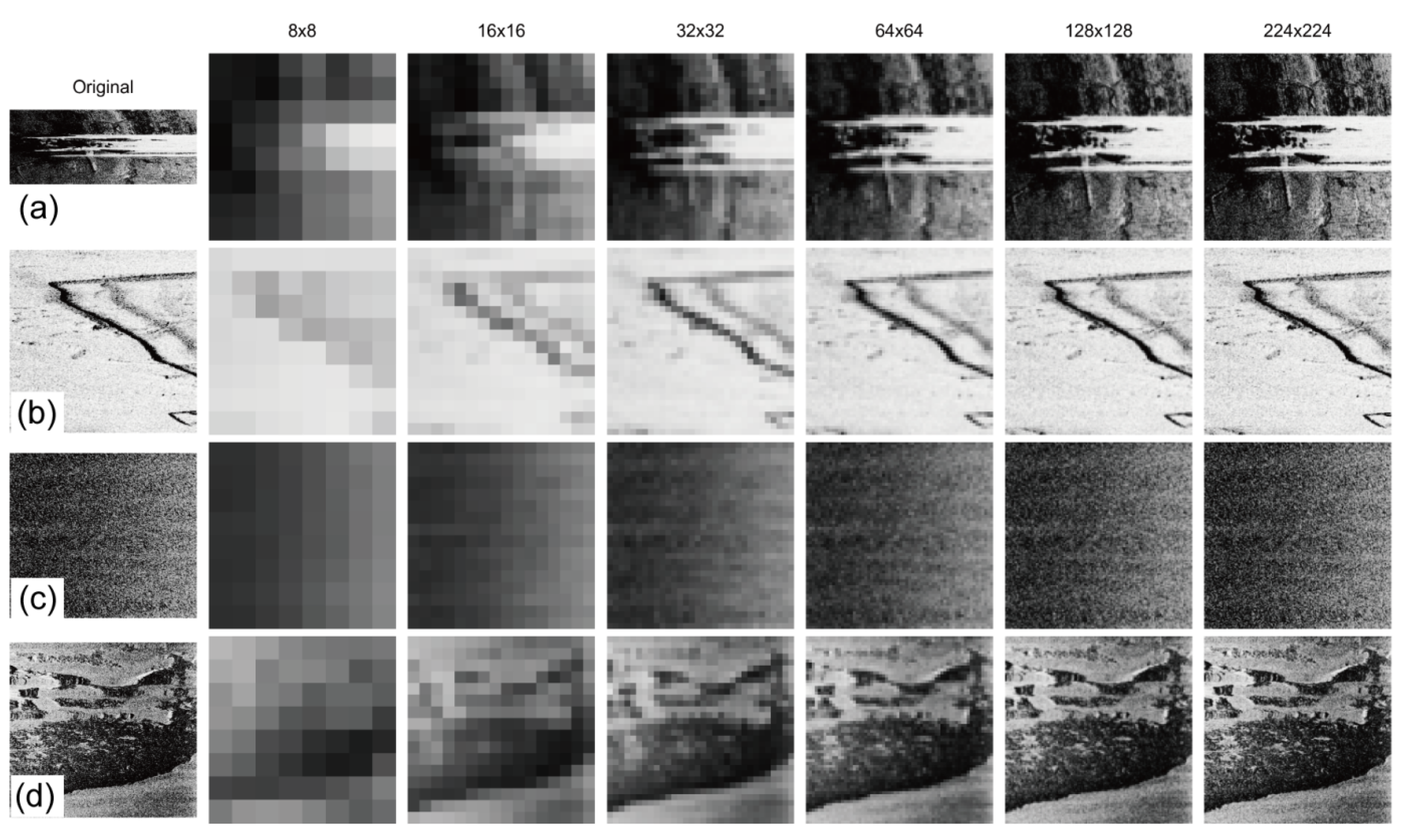
A standardized preprocessing pipeline was applied to all images from both datasets to systematically investigate the impact of resolution. The primary steps involved dynamically resizing the input images during the data loading and model input stages to six target spatial resolutions: 8 × 8, 16 × 16, 32 × 32, 64 × 64, 128 × 128, and 224 × 224 pixels (Figure 2 and Figure 3). This set of resolutions was deliberately chosen to follow a near-power-of-two progression, enabling a systematic, logarithmic-scale analysis of the overall performance trend across a wide range of image scales. The 224 × 224 resolution served as a high-resolution baseline, frequently used with ImageNet pre-trained models, while the lower resolutions, particularly 8 × 8 and 16 × 16, were included to explore performance limits under significant information reduction. Following resizing, images were converted to tensor format and subsequently normalized. For this normalization step, we deliberately used the standard mean and standard deviation values from the ImageNet dataset, rather than statistics derived from the SSS datasets themselves. This is a standard practice in transfer learning, ensuring that the input distribution of our SSS data aligns with that of the original ImageNet pre-training, thereby maximizing the effectiveness of the transferred features. This choice is further supported by existing work [12], which has demonstrated that ImageNet-derived features are highly effective for SSS image analysis, validating the robustness of this approach for our application. Online data augmentation was applied exclusively to the training set images during the training phase to enhance model generalization and robustness; this included random horizontal flipping and random rotation within a range of ±10 degrees. No data augmentation was applied to the validation or test sets during evaluation phases.

2.3. Model Architectures and Selection Strategy

To accommodate the varying information content across different image resolutions and to balance model performance with complexity, this study employed a selection of representative CNN architectures combined with a resolution-adaptive model selection strategy. Four widely recognized CNN models were chosen, spanning a spectrum from lightweight to deep complex networks: MobileNetV2 [22], ResNet18, ResNet50, and ResNet101 [23]. MobileNetV2 is known for its computational efficiency, making it suitable for resource-constrained environments, achieved through depthwise separable convolutions and inverted residuals. The ResNet family effectively addresses vanishing gradients in deep networks via residual connections, with ResNet18, ResNet50, and ResNet101 representing architectures of increasing depth and complexity.

A key aspect of our methodology was the resolution-adaptive model selection strategy, where specific architectures were assigned to different resolution levels based on the pixel characteristics and information density expected at each scale. The rule applied was as follows: MobileNetV2 was used for the extremely low 8 × 8 and 16 × 16 resolutions, as its lightweight structure is well-suited for images with very limited spatial information. For the intermediate and higher resolutions, models from the ResNet family were selected to maintain architectural consistency while varying depth: ResNet18 for 32 × 32, ResNet50 for 64 × 64, and ResNet101 for both 128 × 128 and 224 × 224 resolutions.

This strategy aimed to match the model’s capacity and receptive field to the information density of the input image. For very low resolutions (8 × 8, 16 × 16), where image information is limited, complex deep models risk overfitting and may not leverage their depth effectively; hence, the efficient MobileNetV2 was selected. As resolution increased to 32 × 32 and 64 × 64, providing more detail, model depth and complexity were increased accordingly (ResNet18, ResNet50) to capture richer features. For higher resolutions (128 × 128, 224 × 224), which contain the most information, a larger capacity model (ResNet101) was deemed necessary for comprehensive learning of complex patterns. This tiered selection sought an appropriate balance between performance and efficiency at each resolution level, avoiding model redundancy at low resolutions and insufficient capacity at high resolutions. The primary goal of this selection was not necessarily to identify the absolute highest-performing model for each resolution from all possible CNNs, but rather to use appropriately complex and structurally related models to systematically explore the impact of image resolution on classification accuracy and efficiency within a controlled experimental framework. Further investigation comparing a wider range of CNN architectures was considered beyond the scope of this specific study focused on resolution effects.

All selected models were implemented by fine-tuning ImageNet pre-trained weights. The final fully connected layer was replaced with a new layer matching the target dataset’s class number (four for Marine-PULSE, two for SeabedObjects-KLSG). All model parameters were updated during fine-tuning. For the 8 × 8 resolution, adaptations were made to MobileNetV2, such as adjusting the initial convolutional layer’s stride, to accommodate the minimal input size.

2.4. Experimental Setup and Training Details

All training and evaluation used a consistent environment. A systematic hyperparameter search was conducted by exploring combinations of batch size {16, 32, 64, 128, 256} and initial learning rate {0.0005, 0.001, 0.005}. The specific trials executed for each dataset, covering these hyperparameters across the different resolution-model pairings, are detailed in

Table 1. Hyperparameter search space explored for model optimization.

Trial ID *	Batch Size	Learning Rate	Epochs	Dataset
0411-1	256	0.001	200	Marine-PULSE
0411-2	128	0.001	200	Marine-PULSE
0411-3	64	0.001	200	Marine-PULSE
0411-4	32	0.001	200	Marine-PULSE
0411-5	16	0.001	200	Marine-PULSE
0411-6	128	0.0005	200	Marine-PULSE
0411-7	128	0.005	200	Marine-PULSE
0411-8	256	0.0005	200	Marine-PULSE
0411-9	256	0.005	200	Marine-PULSE
0411-10	64	0.0005	200	Marine-PULSE
0411-11	64	0.005	200	Marine-PULSE
0411-12	32	0.0005	200	Marine-PULSE
0411-13	32	0.005	200	Marine-PULSE
0417-1	64	0.001	200	SeabedObjects-KLSG
0417-2	64	0.0005	200	SeabedObjects-KLSG
0417-3	64	0.005	200	SeabedObjects-KLSG
0417-4	32	0.0005	200	SeabedObjects-KLSG
0417-5	32	0.005	200	SeabedObjects-KLSG
0417-6	32	0.001	200	SeabedObjects-KLSG
0417-7	16	0.001	200	SeabedObjects-KLSG
0417-8	16	0.005	200	SeabedObjects-KLSG
0417-9	16	0.0005	200	SeabedObjects-KLSG

* For resolutions of 8, 16, 32, 64, 128, and 224, the corresponding model strategies are MobileNetV2, MobileNetV2, ResNet18, ResNet50, ResNet101, and ResNet101, respectively.

. The AdamW optimizer was employed for training, configured with a weight decay coefficient of 1 × 10⁻⁴. A constant initial learning rate, selected from the hyperparameter search, was maintained throughout training without an explicit decay schedule. The standard cross-entropy loss function was used for classification task optimization. To mitigate potential model bias arising from the imbalanced class distribution present in both datasets, a weighted loss strategy was employed. Specifically, a weight was assigned to each class, calculated as being inversely proportional to the class frequency in the training set. This ensures that the model incurs a greater penalty for misclassifying samples from minority classes, compelling it to learn their distinguishing features more effectively. This approach addresses the imbalance at the training level without altering the original data distribution through sampling methods.

In addition to the resolution-adaptive strategy described above, a control experiment was conducted to isolate the effect of input resolution and address potential confounding variables arising from changes in model architecture. For this second set of experiments, a fixed ResNet18 architecture was employed across all six resolutions (from 8 × 8 to 224 × 224) for both the Marine-PULSE and SeabedObjects-KLSG datasets. All other experimental parameters, including the hyperparameter search space and training procedure, were kept identical to ensure a fair comparison between the two strategies.

All models were trained for a fixed duration of 200 epochs. A constant initial learning rate (potentially scaled by batch size) was maintained throughout training, without an explicit learning rate decay schedule. Model performance was evaluated on the validation set after each epoch, and the weights corresponding to the best validation performance (highest accuracy) were saved for subsequent final testing on the dedicated test set. To identify the optimal hyperparameters for each resolution-model pairing, a systematic search was conducted. Table 1 documents the full set of experimental trials that constitute this search, detailing the specific combinations of batch size and learning rate explored for each dataset. The final performance metrics reported throughout this paper for any given configuration correspond to the best-performing model selected from these trials, ensuring that our comparisons are based on well-optimized models.

The experiments were executed on a Dell Precision 3660 Tower Workstation (manufactured by Dell Inc., Round Rock, TX, USA; assembled in China) equipped with an Intel Core i9-12900K CPU (Intel Corporation, Santa Clara, CA, USA), 128 GB of DDR5 RAM (brand unspecified), and an NVIDIA GeForce RTX 4090 GPU (NVIDIA Corporation, Santa Clara, CA, USA). The deep learning framework utilized was PyTorch (version, 2.6.0), with Python (version 11.7) as the programming language and CUDA (version 12.6) for GPU acceleration. Automatic Mixed Precision capabilities provided by PyTorch were enabled during training to enhance computational speed and reduce graphics memory consumption.

2.5. Performance Evaluation Metrics

A comprehensive set of metrics, summarized in

Table 2. Evaluation metrics and their physical meanings.

Index	Metric	Physical Meaning
1	Accuracy	Overall proportion of correctly classified samples.
2	Precision (Weighted)	Average precision across classes, weighted by support. Measures the accuracy of positive predictions, considering class imbalance.
3	Recall (Weighted)	Average recall across classes, weighted by support. Measures the ability to find all positive samples, considering class imbalance.
4	F1-score (Weighted)	Harmonic mean of weighted precision and recall, providing a single balanced measure considering class imbalance.
5	Confusion Matrix	Table visualizing classification performance, showing true vs. predicted classes.
6	Parameters (Total)	Total number of parameters in the model, indicating model size and storage needs.
7	Parameters (Trainable)	Number of parameters updated during training, reflecting model learning capacity.
8	GFLOPs	Billions of floating-point operations for one forward pass, indicating computational complexity.
9	Total Training Time	Time required to complete the entire training process (200 epochs) for a specific trial.
10	Average Inference Time	Average time required to process one batch of data during prediction on the test set.

, was employed to evaluate both the classification performance and the computational efficiency across different resolutions and models. Classification performance was primarily assessed using accuracy, precision, recall, and F1-score. For the multi-class Marine-PULSE dataset, weighted-average precision, recall, and F1-score were calculated to account for potential class imbalance, appropriately weighting the contribution of each class by its support and handling potential division by zero scenarios. Confusion matrices were also generated to facilitate detailed error analysis between classes.

Computational efficiency and resource consumption were quantified using several metrics. Model complexity was measured by the total number of parameters and the number of trainable parameters. The computational load for a single forward pass was estimated by counting the Giga Floating Point Operations (GFLOPs) required, based on the model architecture and the specific input resolution. The total training time required to complete the 200 epochs was recorded on the single NVIDIA RTX 4090 GPU setup. Finally, the average inference time, defined as the mean time taken to process one batch of data (in milliseconds), was measured during the evaluation loops using precise CUDA event timing on the same GPU platform, with the batch size corresponding to that used during the training phase of the specific trial.

2.6. Best Trial Selection

For each dataset and each target resolution (ranging from 8 × 8 to 224 × 224), experiments were conducted using the resolution-specific model and applicable hyperparameter combinations detailed in Table 1. After training and evaluating all combinations for a given resolution, the trial that achieved the highest classification accuracy on the independent test set was identified and selected as the “Best Trial” for that specific resolution. Subsequent analyses and results presented in this paper are based on the performance and efficiency data from these selected best trials. This selection process ensures that subsequent analyses focus on the optimized performance achievable under each resolution condition within the explored hyperparameter space.

3. Results

This section presents the experimental results obtained by applying the resolution-adaptive CNN classification methodology to the Marine-PULSE and SeabedObjects-KLSG datasets. The findings focus on the impact of image resolution on model training dynamics, classification performance, and computational efficiency, based on the best-performing hyperparameter configuration identified for each resolution level.

3.1. Training Dynamics of Best Performing Models

Before evaluating the final test performance, the training stability and convergence behavior of the selected best-performing models for each resolution were examined. Figure 4 and Figure 5 illustrate the training and validation accuracy and loss curves over 200 epochs for the Marine-PULSE and SeabedObjects-KLSG datasets, respectively. The specific hyperparameters (batch size and learning rate) that yielded the highest test accuracy for each resolution, and the corresponding accuracy values on the test set, are summarized in

Table 3. Best-performing hyperparameters and associated test accuracy for each resolution.

Resolution (Pixels)	Dataset	Best Test Accuracy (%)	Batch Size	Learning Rate
8 × 8	Marine-PULSE	77.778	64	0.001
16 × 16	Marine-PULSE	84.127	32	0.005
32 × 32	Marine-PULSE	87.302	16	0.001
64 × 64	Marine-PULSE	92.063	32	0.0005
128 × 128	Marine-PULSE	97.619	32	0.0005
224 × 224	Marine-PULSE	94.444	16	0.001
8 × 8	SeabedObjects-KLSG	87.778	16	0.001
16 × 16	SeabedObjects-KLSG	87.778	32	0.005
32 × 32	SeabedObjects-KLSG	91.111	32	0.0005
64 × 64	SeabedObjects-KLSG	93.333	16	0.001
128 × 128	SeabedObjects-KLSG	95.556	32	0.001
224 × 224	SeabedObjects-KLSG	95.556	32	0.0005

.

For the Marine-PULSE dataset, the training accuracy curves (Figure 4a) for all resolution-specific models demonstrate a consistent upward trend, generally saturating or showing minor fluctuations towards the end of the 200 epochs. Models trained on higher resolutions (128 × 128, 224 × 224, using ResNet101) achieve near-perfect training accuracy relatively quickly, while lower-resolution models (especially 8 × 8 and 16 × 16, using MobileNetV2) exhibit slower initial learning but still reach high accuracy levels. Correspondingly, the training loss (Figure 4b) decreases rapidly for all models initially and then continues to decrease at a slower rate, indicating effective optimization. The validation accuracy curves (Figure 4c) show rapid initial improvement followed by stabilization. Notably, models for resolutions 32 × 32 and above achieved validation accuracies exceeding approximately 80–90%, whereas the 8 × 8 and 16 × 16 models plateaued at comparatively lower accuracies. Validation loss (Figure 4d) mirrored this trend, initially decreasing and then stabilizing or slightly increasing for some models in later epochs. This suggests potential mild overfitting but confirms that models learned relevant features before validation performance saturated or degraded.

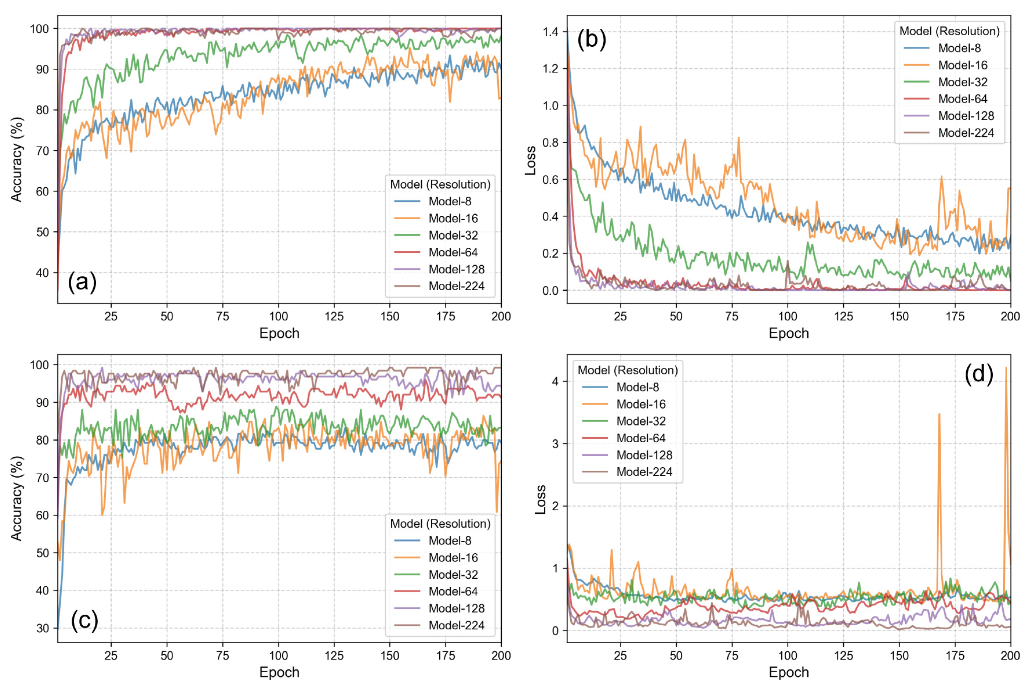
Similar training dynamics are observed for the SeabedObjects-KLSG dataset (Figure 5). The training accuracy (Figure 5a) for all models increases steadily and converges, with higher-resolution models reaching saturation faster. The training loss (Figure 5b) consistently decreases across all resolutions. Validation accuracy (Figure 5c) shows a sharp initial rise followed by stabilization, with models for resolutions 32 × 32 and higher generally achieving better performance than the 8 × 8 and 16 × 16 models. The validation loss (Figure 5d) decreases and then tends to fluctuate or slightly increase, again indicating stable learning followed by potential mild overfitting.

Collectively, these curves (Figure 4 and Figure 5) confirm that the selected models for all tested resolutions achieved stable and effective learning on both datasets. This provides confidence that the subsequent evaluations of test set performance and computational efficiency are based on well-trained models.

3.2. Impact of Resolution on Classification Performance and Behavior

The core objective of this study was to assess how reducing image resolution affected classification performance. Key classification metrics (accuracy, F1-score, precision, recall) achieved by the best-performing models on the test set for the Marine-PULSE and SeabedObjects-KLSG datasets, respectively, across the six target resolutions, are presented in

Table 4. Performance metrics for the Marine-PULSE dataset across different resolutions.

Resolution	Accuracy (%)	Precision (Weighted)	Recall (Weighted)	F1-Score (Weighted)
8 × 8	77.8	0.78	0.78	0.77
16 × 16	84.1	0.84	0.84	0.84
32 × 32	87.3	0.88	0.87	0.87
64 × 64	92.1	0.92	0.92	0.92
128 × 128	97.6	0.98	0.98	0.98
224 × 224	94.4	0.95	0.94	0.94

and

Table 5. Performance metrics for the SeabedObjects-KLSG dataset across different resolutions.

Resolution	Accuracy (%)	Precision (Weighted)	Recall (Weighted)	F1-Score (Weighted)
8 × 8	87.8	0.86	0.88	0.87
16 × 16	87.8	0.86	0.88	0.85
32 × 32	91.1	0.91	0.91	0.9
64 × 64	93.3	0.94	0.93	0.94
128 × 128	95.6	0.95	0.96	0.95
224 × 224	95.6	0.96	0.96	0.95

.

As shown in the tables, a clear trend of performance degradation with decreasing resolution was evident for both datasets. On the Marine-PULSE dataset (Table 4), accuracy peaked at 97.62% for the 128 × 128 resolution and dropped to 77.78% at the 8 × 8 resolution. For SeabedObjects-KLSG (Table 5), the highest accuracy of 95.56% was achieved at both 128 × 128 and 224 × 224 resolutions, decreasing to 87.78% at the 8 × 8 and 16 × 16 resolutions. The F1-score, a metric that balances precision and recall, exhibited a similar pattern, confirming the negative impact of lower resolution on overall classification performance.

To identify the minimum resolution required to maintain specific performance levels, we analyzed the accuracy results. For the Marine-PULSE dataset, accuracies above 90% were maintained down to the 64 × 64 resolution (92.06%). An accuracy level above 80% was sustained down to the 16 × 16 resolution (84.13%). For the SeabedObjects-KLSG dataset, performance is generally higher at lower resolutions; accuracy remained above 90% down to the 32 × 32 resolution (91.11%), and accuracies above 85% were achieved even at the lowest tested resolutions (87.78% for 8 × 8 and 16 × 16). These results suggested that for applications requiring at least 90% accuracy, a resolution of 64 × 64 might suffice for Marine-PULSE, while 32 × 32 could be adequate for SeabedObjects-KLSG. If an 80–85% accuracy threshold was acceptable, significantly lower resolutions like 16 × 16 could have been considered for both datasets.

An anomalous observation was noted for the Marine-PULSE dataset (Table 4), where the performance metrics, including accuracy and F1-score, exhibited a slight decrease when transitioning from the 128 × 128 resolution to the 224 × 224 resolution, despite both employing the same ResNet101 architecture. This finding, which differs from the general expectation that higher resolution should yield superior performance, is further analyzed in the Section 4. To understand the specific classification behaviors underlying these overall performance changes, confusion matrices for each resolution were generated, as shown in Figure 6 (Marine-PULSE) and Figure 7 (SeabedObjects-KLSG).

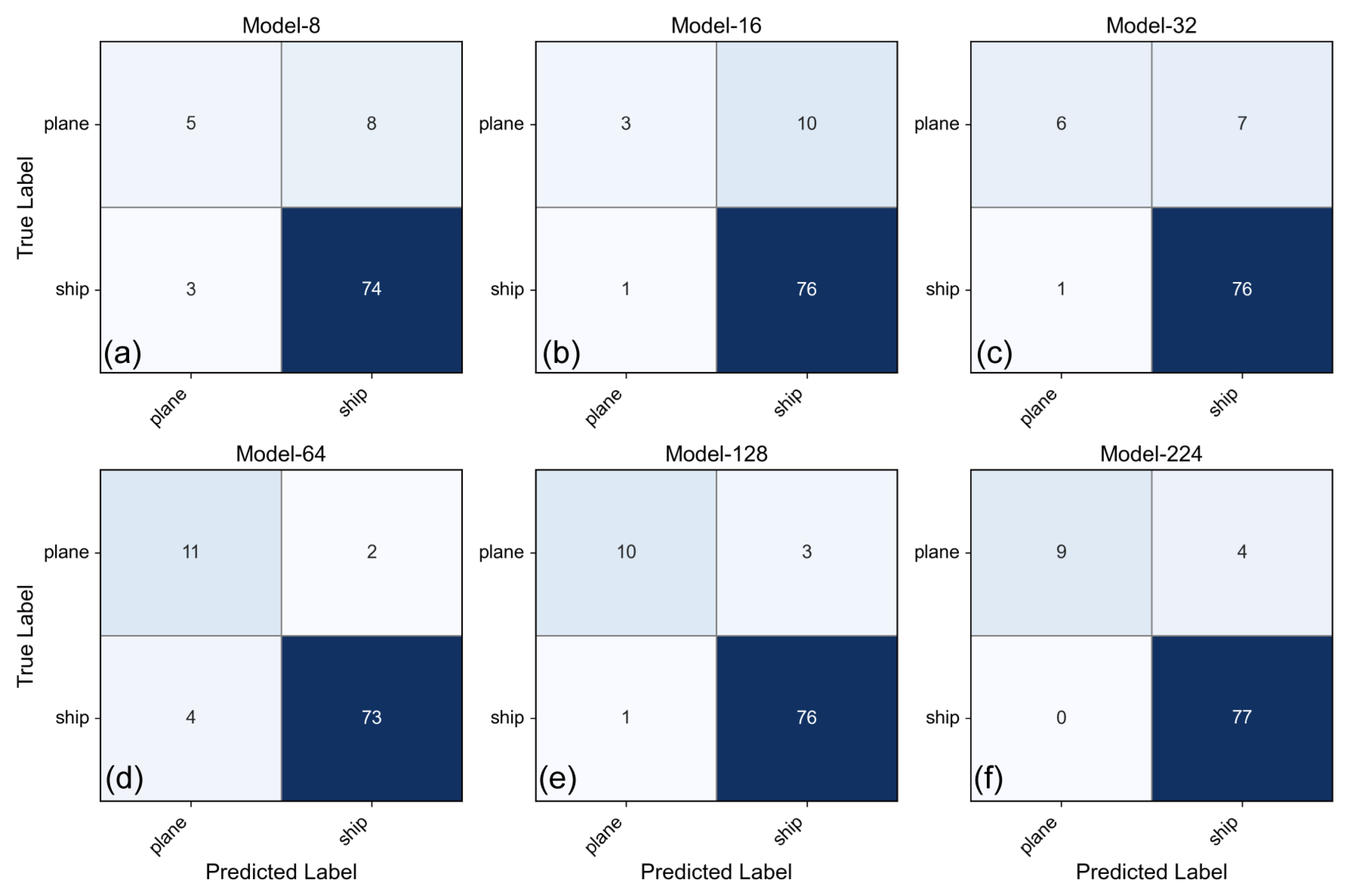
At higher resolutions (e.g., 224 × 224, 128 × 128), the confusion matrices for both datasets showed strong diagonal dominance, indicating high correct classification rates across most classes. However, as resolution decreased, off-diagonal elements became more prominent, signifying increased confusion between classes. For the Marine-PULSE dataset (Figure 6), significant confusion emerged between the POC and URM classes, particularly at resolutions of 32 × 32 and below. Misclassifications involving the SS class, confusing it primarily with POC and URM, also increased notably at the lowest resolutions (8 × 8, 16 × 16). This suggested that the reduction in resolution hindered the model’s ability to distinguish features specific to these geologically related or structurally similar categories. For the SeabedObjects-KLSG dataset (Figure 7), increased confusion between the “plane” and “ship” classes was observed at lower resolutions, especially at 16 × 16 and 8 × 8, indicating that critical shape or structural details distinguishing these objects were lost or degraded. The trends in precision and recall presented in Figure 6b,c and Figure 7b,c further corroborated these findings, showing decreased recall and/or precision for the specific classes identified as becoming more confused at lower resolutions.

3.3. Impact of Resolution on Computational Efficiency and Cross-Dataset Comparison

This subsection evaluated the influence of image resolution reduction, combined with the adaptive model strategy, on computational efficiency metrics and provided a comparative analysis between the two datasets.

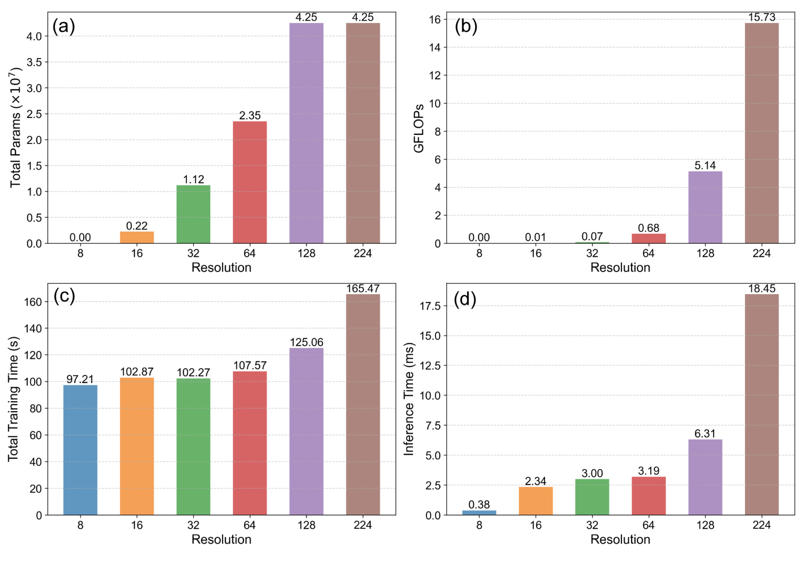
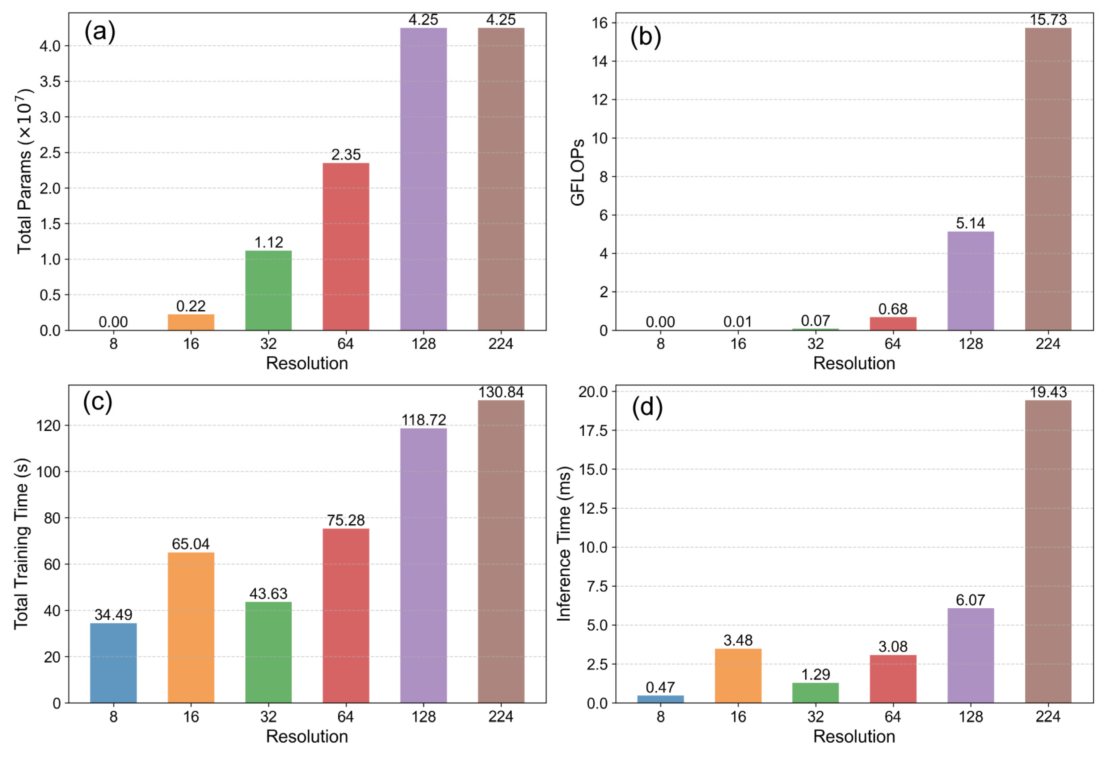
A substantial improvement in computational efficiency and a reduction in resource usage were consistently observed as image resolution decreased for both datasets, as illustrated in Figure 8 and Figure 9. The metrics, including total model parameters, GFLOPs, total training time, and average inference time, all exhibited significant downward trends corresponding to the reduction in resolution and the associated shift towards less complex models (from ResNets to MobileNetV2). Notably, the transition points in the model selection strategy (e.g., from ResNet18 at 32 × 32 to MobileNetV2 at 16 × 16) corresponded to particularly sharp drops in parameters (Figure 8a and Figure 9a) and GFLOPs (Figure 8b and Figure 9b). This highlighted the considerable efficiency gains achieved by employing lightweight architectures at very low resolutions. The time-related metrics also showed substantial reductions; total training time (Figure 8c and Figure 9c) and average inference time (Figure 8d and Figure 9d) decreased by orders of magnitude from the highest (224 × 224) to the lowest (8 × 8) resolution, emphasizing the practical benefits for training duration and potential real-time application speed.

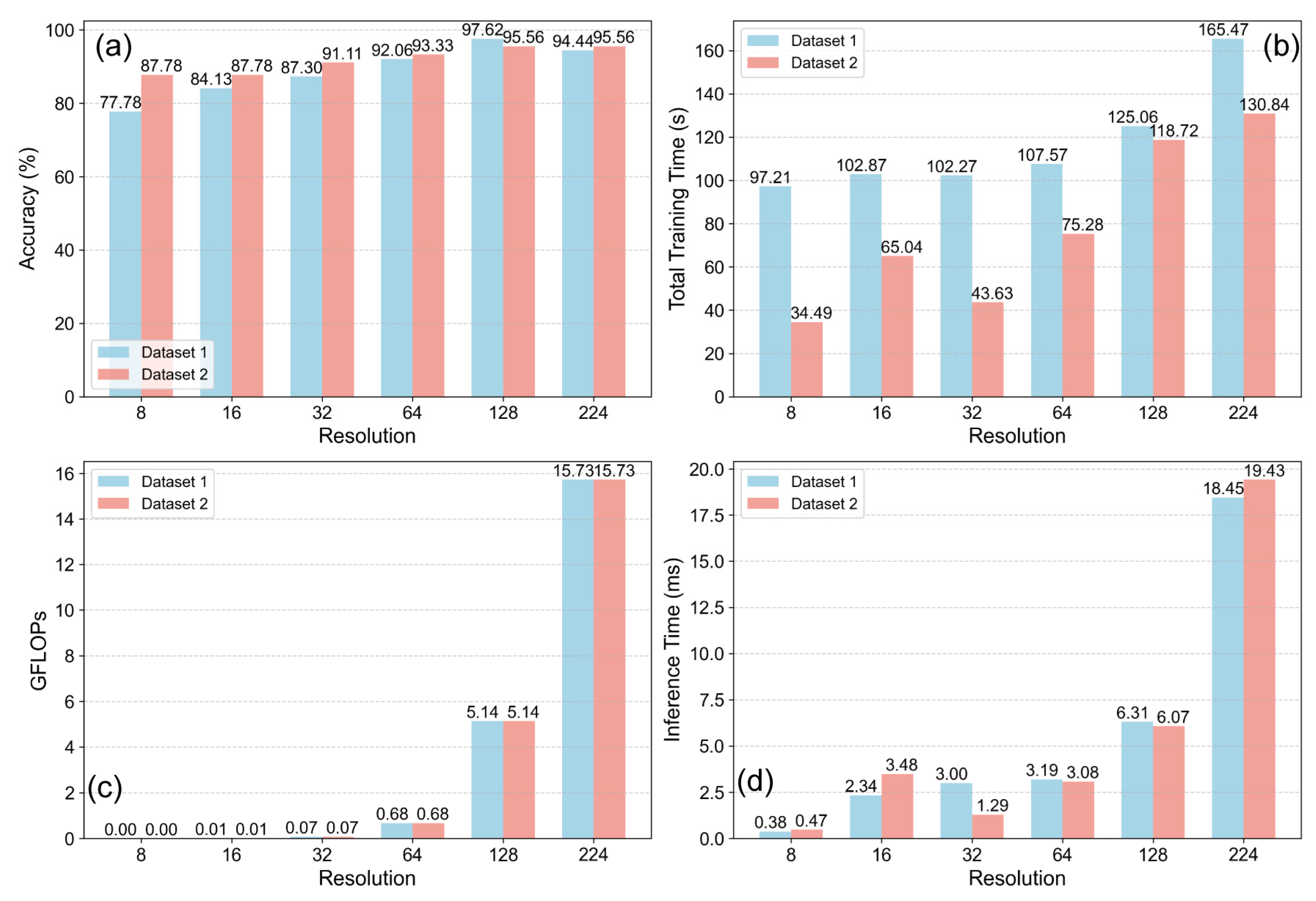
A direct comparison of key metrics between the two datasets is presented in Figure 10. As expected from the identical model selection strategy, the GFLOPs required at each corresponding resolution were nearly identical for both datasets (Figure 10c). In contrast, practical time-based metrics and classification accuracy revealed clear, task-dependent differences. The total training time (Figure 10b) and average inference time (Figure 10d) were consistently lower for the SeabedObjects-KLSG dataset compared to the Marine-PULSE dataset. This suggested that the simpler two-class problem of SeabedObjects-KLSG might have allowed for faster convergence during training and potentially less computational overhead per sample during inference, despite using models of similar theoretical complexity (GFLOPs) at each resolution. The accuracy comparison (Figure 10a), consistent with observations in Section 3.2, showed that the SeabedObjects-KLSG task yielded higher accuracy, particularly at lower resolutions, than the more complex four-class Marine-PULSE task, with the performance gap being most pronounced at lower resolutions. Collectively, these results indicate that while the efficiency gains from resolution reduction are universally applicable, the precise impact on accuracy and processing time is highly dependent on the intrinsic complexity of the classification task.

To provide a more practical assessment of deployment feasibility beyond theoretical metrics, we benchmarked the inference latency of select low-resource configurations. Specifically, the pre-trained MobileNetV2 model for 16 × 16 resolution and the ResNet18 model for 32 × 32 resolution were tested. The benchmark was conducted on a ThinkPad X1 Carbon laptop (Lenovo, Beijing, China; assembled in China), using its Intel i5-1135G7 processor constrained to a single-core mode to represent a significantly resource-limited hardware scenario. For each model, the average inference time was calculated over 1000 runs on a single input image, following an initial 100-run warm-up period to ensure stable performance. The results are summarized in

Table 6. CPU inference latency benchmark on a low-power device.

Model	Resolution	Dataset	Avg. Inference Time (ms/Image)
MobileNetV2	16 × 16	Marine-PULSE	5.8
ResNet18	32 × 32	Marine-PULSE	25.6

.

The benchmark demonstrates that even in this highly constrained, low-power test environment, the lightweight models achieve inference times well within the requirements for most real-time applications.

3.4. Comparison with a Fixed-Architecture Baseline

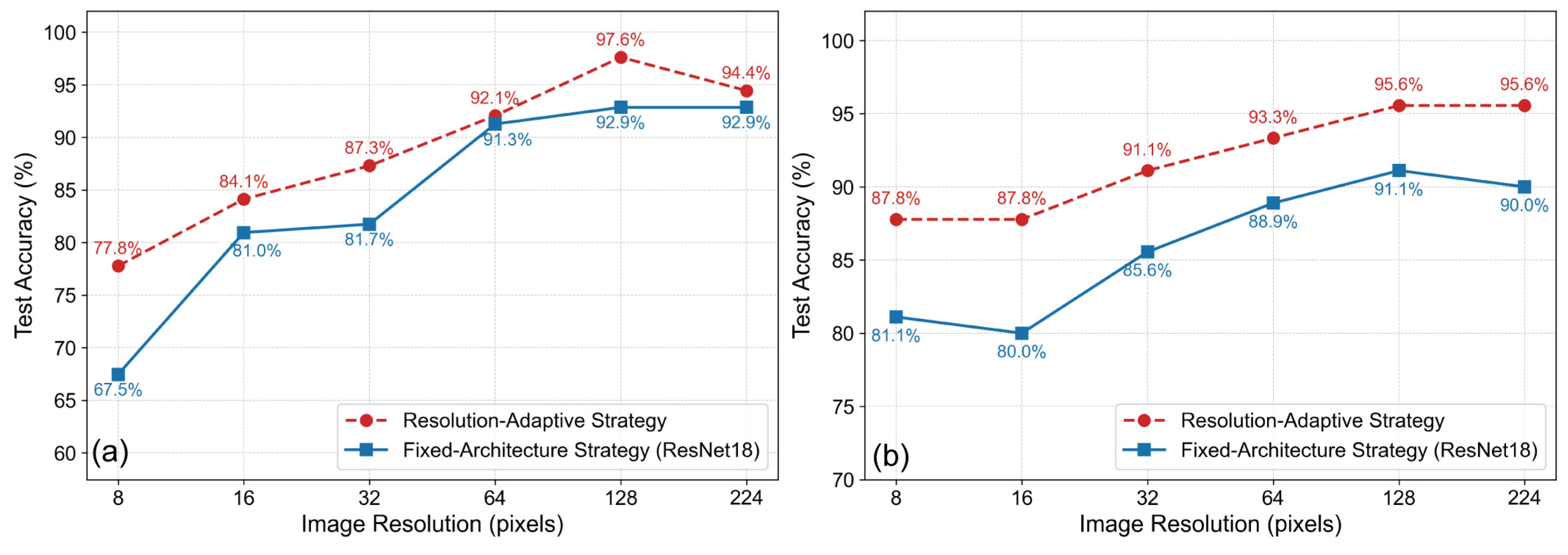
To isolate the effect of input resolution from model capacity, a control experiment using a fixed ResNet18 architecture was conducted. Figure 11 presents a direct comparison of the test accuracy between our proposed resolution-adaptive strategy and this fixed-architecture baseline across both datasets.

As illustrated in Figure 11a for the Marine-PULSE dataset, the performance of the fixed-architecture strategy improves steadily with resolution, increasing from 67.5% at 8 × 8 to a peak accuracy of 92.9% at 128 × 128 pixels. In contrast, the resolution-adaptive strategy consistently outperforms this baseline across all resolutions. Notably, the performance gap is most pronounced at lower resolutions (e.g., 77.8% vs. 67.5% at 8 × 8) and at the optimal high resolution of 128 × 128, where the adaptive strategy achieves a peak accuracy of 97.6%, significantly higher than the 92.9% achieved by the fixed model.

A similar trend is observed in Figure 11b for the simpler, two-class SeabedObjects-KLSG dataset. The resolution-adaptive strategy again demonstrates superior accuracy compared to the fixed-architecture baseline at every resolution level. For instance, at a resolution of 64 × 64, the adaptive strategy yields an accuracy of 93.3%, whereas the fixed ResNet18 model only reaches 88.9%. While both strategies show performance improvements with an increasing resolution up to 128 × 128, the adaptive approach consistently maintains a higher performance ceiling.

Collectively, these results from both datasets empirically demonstrate that intelligently matching model capacity to the information density of the input image is a more effective approach than applying a single, fixed-complexity model across all resolutions. The resolution-adaptive strategy not only achieves higher peak accuracy but also provides better performance at the critical low-resolution end of the spectrum.

4. Discussion

4.1. Interpretation of the Accuracy–Efficiency Trade-Off at Different Resolutions

This study undertook an examination of the inherent trade-off between classification accuracy and computational efficiency when varying image resolution in SSS image analysis. Figure 12 quantitatively demonstrates this relationship for the Marine-PULSE and SeabedObjects-KLSG models, mapping accuracy against both computational load (GFLOPs) and total training time. The results revealed a consistent pattern: decreasing resolution led to substantial gains in computational efficiency but at the cost of reduced classification accuracy.

Importantly, the analysis extended beyond simply identifying the maximum achievable accuracy to investigate the feasibility of operating at reduced computational costs while maintaining pre-defined performance thresholds. For both datasets, achieving the highest accuracy (referring to values like 97.62% for Marine-PULSE and 95.56% for SeabedObjects-KLSG, as reported in the Section 3) necessitated higher resolutions (e.g., 128 × 128 or 224 × 224, corresponding to higher computational loads). However, if application constraints permit a slight decrease in performance, significant resource savings are possible. Specifically, to maintain accuracy above the 90% level, the results suggested that training with image resolutions of 64 × 64 or potentially 32 × 32 is sufficient, representing a considerable reduction in computational demand compared to using the highest resolutions. If an accuracy threshold of approximately 80% is acceptable, the data indicated that even lower resolutions, potentially around 16 × 16 (corresponding to computational loads near eight GFLOPs for the associated MobileNetV2 model), could be viable, further minimizing resource usage. Similar trends were observed for training time, where lower resolutions offered dramatically faster training as evidenced by the significantly reduced total training times reported in Section 3.3. This tiered analysis provides actionable guidance for selecting the minimum required resolution based on application-specific accuracy needs.

To further illustrate the practical implications for system deployment,

Table 7. Illustrative computational configurations for target test set accuracy levels.

Target Accuracy Level	Typical Resolution(s) from This Study	Associated Model(s) from This Study	Estimated Computational Load Category (Based on GFLOPs)	Illustrative GPU Tier Example	Primary Suitability
Maximum Accuracy Achieved	128 × 128–224 × 224	ResNet101	High	NVIDIA RTX 4090 24 G	Demanding training; maximum performance inference for critical applications.
>90% Accuracy	32 × 32–64 × 64	ResNet18/ResNet50	Medium	NVIDIA RTX 4060 8 G	Balanced performance for desktop/server applications; feasible model training.
>80% Accuracy	8 × 8–16 × 16	MobileNetV2	Low	Lower-end GPU/Potent CPU	Highly resource-constrained environments (e.g., AUVs, edge devices) for inference.

summarizes indicative computational configurations tailored to different target accuracy levels, based on the findings of this study. These examples map achieved accuracies to the resolutions and model types used, along with an estimation of the class of GPU that might be suitable.

As Table 4 indicates, achieving the maximum test set accuracy observed in this study (e.g., >95%), which typically involved 128 × 128 or 224 × 224 resolutions with the ResNet101 architecture, generally necessitates a high-performance GPU. An NVIDIA RTX 4090 with 24 GB of VRAM, similar to the one used in this study’s experimental setup, would be representative for handling the associated model complexity and larger input data, especially for efficient training and swift high-accuracy inference. For applications requiring a test set accuracy consistently above 90% (achievable in this study with resolutions like 64 × 64 using ResNet50 or 32 × 32 using ResNet18, if these yield >90% but less than maximum), a mid-range GPU like an NVIDIA RTX 4060 with 8 GB of VRAM could provide an adequate balance of performance and cost. Such configurations are suitable for many desktop or server-based analytical tasks and allow for feasible training durations. Finally, if a test set accuracy above 80% meets the operational requirements (corresponding to resolutions like 8 × 8 or 16 × 16 with the lightweight MobileNetV2 model), the computational demands become minimal. Inference tasks at this level could potentially be handled by lower-specification GPUs, integrated graphics, or even capable CPUs, making this approach highly suitable for deployment on resource-constrained platforms such as AUVs or edge computing devices. It is important to note that these GPU tiers are illustrative examples; actual VRAM and processing requirements will vary based on factors like batch size during inference or training, specific framework overheads, and software optimizations. Nevertheless, this mapping provides tangible guidance on the hardware implications of selecting different operational points on the accuracy–efficiency spectrum.

The underlying cause for accuracy degradation at lower resolutions is the loss of discriminative information. As resolution decreases, fine details and subtle textures necessary for distinguishing between classes become obscured. This information loss directly impacts the model’s ability to learn effective representations. Notably, the impact of this loss differed between the two datasets, reflecting their varying classification complexities. Marine-PULSE, with its more challenging four-class problem, exhibited greater sensitivity to resolution reduction, showing a steeper decline in accuracy. This is logically consistent, as finer details are likely more pertinent for differentiating between four similar underwater object classes. Conversely, the simpler two-class SeabedObjects-KLSG dataset demonstrated more robustness, maintaining higher relative accuracy at lower resolutions, likely because the broader distinguishing features remained more intact. This suggests a key principle: the acceptable lower bound for image resolution in SSS analysis is intrinsically linked to the complexity of the classification task itself.

4.2. Physical Interpretation of Resolution Impact: Feature Scale, SSS Image Characteristics, and Task Complexity

The degradation in classification accuracy observed at lower image resolutions fundamentally stems from the loss of discriminative information critical for class differentiation. As resolution decreases, fine details and subtle textures become obscured, directly impacting the model’s ability to learn effective feature representations. However, the precise nature of this impact and the optimal resolution are deeply intertwined with the unique characteristics of SSS imagery, the scale of relevant features, and the complexity of the classification task itself.

Generally, higher image resolution is presumed to yield superior classification accuracy because it provides a richer, more detailed representation of the scene. More pixels per unit area allow for the potential capture of finer textural variations, sharper object boundaries, and smaller distinguishing features that might be crucial for separating classes. This aligns with the principle that a higher sampling rate (resolution) can resolve higher frequency components (finer details) of an input signal. For deep learning models, this increased detail offers more raw information from which to learn discriminative features.

However, this study observed a notable anomaly where this general trend did not hold: for the Marine-PULSE dataset, the 128 × 128 resolution yielded higher accuracy than the 224 × 224 resolution when using the same ResNet101 architecture. This counter-intuitive result highlights a critical principle in applying deep learning to physical sensing data: the highest resolution does not necessarily equate to the most useful information for a given task. SSS imagery at 224 × 224 provides a very high-fidelity representation of the seafloor, but this detail includes inherent, high-frequency speckle noise. From a hydrographic survey perspective, while this speckle is a real physical artifact of coherent acoustic interference, it often acts as noise that can obscure the larger, structurally significant features needed to differentiate between macro-scale classes like pipelines and seabed mounds. Effectively, overly high resolution can decrease the signal-to-noise ratio of the features relevant to the classification task. In contrast, appropriately reducing the resolution to 128 × 128 acts as an implicit spatial averaging filter. This process naturally suppresses the fine-grained speckle noise while preserving the more robust, lower-frequency features of the targets. By providing the model with this “pre-filtered,” less ambiguous data, the 128 × 128 resolution allows the network to learn a more generalizable representation based on the essential characteristics of the targets, rather than overfitting to the stochastic noise patterns present in the higher-resolution images.

The differing sensitivity of the two datasets to resolution changes underscores the importance of feature scale relative to task complexity. The ability of a model to maintain accuracy at reduced resolutions implies that the essential, class-defining features are large or robust enough to remain discernible even after downsampling. For the simpler two-class SeabedObjects-KLSG dataset, distinguishing between “ship” and “plane” likely relies on global morphological characteristics (e.g., overall shape, length-to-width ratio) that are relatively large-scale and distinct. These coarse features are inherently more resilient to resolution reduction. Conversely, the more complex four-class Marine-PULSE dataset involves finer distinctions between classes such as “POC”, “URM”, and “SS”. Differentiating these may depend on subtle textural variations, the precise geometry of linear features, or the detailed characteristics of acoustic shadows—all of which are high-frequency details vulnerable to information loss at lower resolutions. When a task requires separating multiple classes with more subtle inter-class differences, a higher resolution is typically necessary to preserve these nuanced discriminative features. Thus, the more complex the classification problem (i.e., more classes, or classes with less distinct features), the higher the image resolution generally required to maintain a target level of accuracy, as the model needs more detailed information to resolve ambiguities.

These interpretations lead to important considerations for future SSS image model training and prediction strategies. The findings of this study strongly suggest that defaulting to the highest possible image resolution is not necessarily the optimal approach. Instead, a multi-resolution evaluation, as conducted herein, should be considered a more robust methodology. The choice of an optimal resolution is not absolute but rather a function of the specific SSS targets, the inherent complexity of the classification task (number and similarity of classes), the specific characteristics of the SSS data (noise levels, feature scales), the chosen model architecture, and the desired accuracy versus computational efficiency trade-off. Therefore, rather than a one-size-fits-all rule, it is recommended that practitioners first assess the scale of critical distinguishing features for their specific application. An iterative approach, starting with a moderate resolution and progressively exploring higher or lower resolutions based on initial performance and computational budgets, is likely to yield a more tailored and efficient solution. This study provides a framework for such an informed selection, emphasizing that the “best” resolution is one that meets the application’s accuracy requirements while respecting its computational constraints.

4.3. Contextualization of the Model Strategy and Comparison with Related Work

The study employed a resolution-adaptive model selection strategy, matching computationally lighter architectures (e.g., MobileNetV2) to lower resolutions and more complex ones (e.g., ResNet101) to higher resolutions. This approach aligns with the principle of resource optimization, demonstrating that simpler models can effectively process lower-information inputs without the computational overhead or potential overfitting associated with overly complex models.

It is important to clarify the role of MobileNetV2 as the exemplar lightweight architecture. While numerous alternatives like ShuffleNet and EfficientNet exist, the objective of this study was not to conduct an exhaustive search for the single optimal lightweight model. Rather, MobileNetV2 was chosen as a representative and widely adopted baseline to validate the principle that employing such architectures at very low resolutions is a feasible and effective strategy within our accuracy–efficiency framework. The methodological framework itself is model-agnostic and can be readily applied to other models in future, application-specific optimizations.

It is important, however, to position this strategy within the broader research landscape. The selected model suite (MobileNetV2, ResNet variants) represents a practical choice but is not exhaustive. We acknowledge that alternative architectures, such as the GoogleNet highlighted by Du [24] for the SeabedObjects-KLSG dataset, might yield superior accuracy or efficiency metrics. Nonetheless, this study’s primary contribution is not predicated on identifying the single optimal architecture. Rather, it centers on establishing and validating a methodological framework for evaluating the accuracy–efficiency trade-off inherent in resolution adaptation.

This framework provides a systematic means to quantify how performance scales with computational resources as resolution changes—a principle applicable across diverse model architectures, including future ones. While comparative model studies like Du [24] offer valuable benchmarks for specific model performance, this work provides a complementary, broader perspective focused on the strategic management of computational resources via input resolution. This methodological contribution holds particular relevance for practical deployment scenarios, especially those involving resource-constrained platforms like embedded systems on AUVs, where balancing performance and efficiency is paramount.

The control experiment, which compared our resolution-adaptive strategy against a fixed ResNet18 architecture (Figure 11), provides empirical validation for this approach. The results reveal that the superiority of the adaptive strategy is rooted in the principle of matching model capacity with the information density of the input data. At lower resolutions, lightweight models (e.g., MobileNetV2) outperform the fixed ResNet18 because their reduced complexity is better suited to the sparse information, mitigating the risk of overfitting. Conversely, at higher resolutions, deeper models (e.g., ResNet101) surpass the fixed ResNet18 by leveraging their greater capacity to exploit the rich details that a model with a fixed, medium capacity cannot. Therefore, the supplementary experiment confirms that the resolution-adaptive strategy is not a methodological compromise but rather a more effective and principled approach to optimizing performance across the entire resolution spectrum.

It is also critical to distinguish the contribution of this study from the predominant focus of the existing literature. Much of the prior research in SSS image classification has concentrated on proposing novel, often more complex, model architectures to achieve state-of-the-art accuracy, typically at a fixed high resolution. In contrast, the primary contribution of this work is not a new architecture, but rather a novel methodological framework for systematic evaluation. The advantage of this approach is threefold: First, it provides the first quantitative, multi-resolution analysis of the accuracy–efficiency trade-off, moving beyond anecdotal observations. Second, it shifts the research objective from pursuing maximum performance to providing a practical, data-driven basis for making informed decisions in resource-constrained scenarios. Finally, this framework offers actionable guidance for engineers and operators, which is a critical but often overlooked aspect in purely performance-oriented studies.

4.4. Practical Considerations for Real-World Application and Limitations

Beyond the quantitative analysis of the accuracy–efficiency trade-off, it is crucial to consider the practical implications and limitations of these findings in real-world operational scenarios. Our study identifies an optimal downsampling resolution that balances overall accuracy and computational cost, yet its application requires careful consideration of the specific mission objectives and the nature of the targets.

A key consideration is the model’s capability for fine-grained discrimination at the proposed optimal resolutions. For instance, distinguishing between similar object types, such as a shipwreck versus an airplane wreck, is a task that falls into the domain of fine-grained visual classification. The public datasets used in this study, including SeabedObjects-KLSG, group various types of wrecks into a single “Wreck” category. Consequently, the models were trained to solve a general object classification task, not to perform such intra-class differentiation. Achieving this level of detail would necessitate a different dataset with more granular labels and potentially more complex model architectures, which is beyond the scope of our current investigation.

Furthermore, the physical size of the target object critically affects the effectiveness of any chosen resolution threshold. The optimal resolution identified in our work represents a balanced trade-off for the average performance across all objects in the datasets. There is an inherent relationship where larger objects are more resilient to resolution reduction, whereas smaller objects may lose their defining features and become undetectable at lower resolutions. Therefore, the choice of an operational resolution must be mission-dependent. For instance, in a search mission for small, critical targets (e.g., unexploded ordnance), a higher resolution would be necessary. Conversely, for large-scale seabed mapping or searching for large wrecks, a lower-resolution threshold offers a highly efficient solution. Our quantitative framework is thus presented not as a single fixed solution, but as an actionable guide for operators to make informed, mission-specific decisions on the accuracy–efficiency trade-off.

Furthermore, to directly address the concern of deployment feasibility, we performed a practical validation of inference speed. This benchmark, conducted on a ThinkPad X1 Carbon laptop (Intel i5-1135G7, single-core mode), involved measuring the average latency over 1000 inference cycles for the pre-trained 16 × 16 MobileNetV2 model. As shown in Table 4, this configuration achieved an average inference time of just 5.8 ms. This processing speed (equivalent to ~172 frames per second) far exceeds the typical real-time requirements for AUV survey missions. It is important to note that this test represents a conservative baseline; the performance on a dedicated embedded AI accelerator (e.g., NVIDIA Jetson series), commonly found on modern AUVs, is expected to be substantially better. Therefore, this empirical evidence provides strong validation that the low-resolution strategies identified in this study are not merely theoretical but are indeed a viable and effective solution for real-world deployment on resource-constrained platforms.

4.5. Implications and Future Directions

The physical interpretations, combined with the empirical findings of this study, lead to important considerations for future SSS image model training and prediction strategies. The findings strongly suggest that defaulting to the highest possible image resolution is not necessarily the optimal approach. Instead, a multi-resolution evaluation, as conducted herein, should be considered a more robust methodology. The choice of an optimal resolution is not absolute but rather a function of the specific SSS targets, the inherent complexity of the classification task (number and similarity of classes), the specific characteristics of the SSS data (noise levels, feature scales), the chosen model architecture, and the desired accuracy versus computational efficiency trade-off. An iterative approach, starting with a moderate resolution and progressively exploring higher or lower resolutions based on initial performance and computational budgets, is likely to yield a more tailored and efficient solution. This study provides a framework for such an informed selection, emphasizing that the “best” resolution is one that meets the application’s accuracy requirements while respecting its computational constraints.

The quantitative insights into the accuracy–efficiency trade-off presented here also carry significant implications for the design and deployment of real-world SSS image classification systems. Practitioners can leverage this framework to make informed decisions, selecting the minimal resolution that meets the target accuracy for their specific application, thereby optimizing resource utilization. For instance, onboard processing systems on AUVs or ROVs, often limited by power and computational capacity, could operate at carefully chosen lower resolutions (e.g., 32 × 32 or 64 × 64) to achieve near real-time performance with acceptable accuracy, significantly enhancing mission endurance and autonomy.

However, this study also underscores the limitations of applying generic computer vision models to SSS data and points towards necessary future research directions. A key direction is the development of novel deep learning architectures specifically engineered for the unique challenges of side-scan sonar imagery. Standard CNNs, designed primarily for optical images, often do not adequately capture the complex spatial relationships, handle the high levels of speckle noise, or interpret the acoustic shadow information inherent in SSS data. Architectures tailored to these characteristics hold the potential for substantial gains in both accuracy and robustness, potentially even mitigating the performance drop observed at lower resolutions. Investigating methods for explicitly improving low-resolution SSS image representation, perhaps through specialized data augmentation or integrated super-resolution techniques within these new models, represents a complementary path. Furthermore, refining the trade-off analysis itself by exploring finer resolution intervals and incorporating key deployment metrics like energy consumption and memory footprint will be vital for evaluating and optimizing these future SSS-specific models. Extending the application of this trade-off methodology to more complex underwater tasks, such as object detection and semantic segmentation, is also warranted. Finally, an essential step towards establishing the broader applicability of these findings involves rigorous validation of the observed trade-off principles and the performance of any new methods across a more diverse range of SSS datasets, encompassing varied seafloor types, environmental conditions, and target objects. Such validation is necessary to confirm the generalizability and practical utility of the proposed approaches.

5. Conclusions

This research systematically evaluated the impact of input image resolution on the accuracy and computational efficiency of deep learning models for SSS image classification. The study provides quantitative insights into managing the inherent trade-offs for practical applications. The key conclusions are as follows:

(1)

Input resolution significantly influences model classification accuracy. Generally, higher resolutions yield higher accuracy, as observed across resolutions from 8 × 8 up to 128 × 128 pixels. However, this trend is not strictly monotonic; for the Marine-PULSE dataset, the accuracy achieved at 224 × 224 resolution was slightly lower than at 128 × 128, suggesting that simply maximizing resolution does not guarantee optimal performance, potentially due to increased noise or model limitations in handling ultra-fine details in SSS data.

(2)

Computational requirements are driven by both input resolution and model complexity. To achieve optimal classification accuracy, it is generally necessary to match model capacity with the information density of the input; higher-resolution images typically require deeper, more complex models to effectively process their detailed features. Our resolution-adaptive strategy embodies this principle. Consequently, the inherent increase in computational load from higher resolution is substantially amplified when employing this strategy, leading to a significant rise in GFLOPs, total training time, and inference time, particularly when transitioning to the deepest models.

(3)

It is feasible to achieve acceptable accuracy with significantly reduced computational cost by selecting an appropriate lower resolution. For applications requiring over 90% accuracy, resolutions of 64 × 64 (for Marine-PULSE) or 32 × 32 (for SeabedObjects-KLSG) were sufficient. If an accuracy threshold around 80–85% is adequate, resolutions as low as 16 × 16 could be employed for both datasets. This provides a basis for selecting the minimum required resolution tailored to specific engineering accuracy demands and available hardware capabilities.

(4)

The optimal balance between resolution, accuracy, and efficiency is task-dependent, influenced by the complexity of the dataset. The simpler two-class SeabedObjects-KLSG classification task consistently allowed for lower resolutions to meet specific accuracy targets compared to the more challenging four-class Marine-PULSE task, indicating that less complex datasets are more amenable to resolution reduction strategies.

(5)

Limitations exist in applying standard vision models directly to SSS data due to its unique characteristics like high noise levels, geometric distortions, and acoustic shadows. Future work should therefore prioritize the development of novel deep learning architectures specifically designed for SSS imagery, potentially incorporating techniques to enhance low-resolution performance. Validating these findings and new methods across a wider variety of SSS datasets is also an essential next step to ensure generalizability and practical utility.