Article

An Accurate LiDAR-Inertial SLAM Based on Multi-Category Feature Extraction and Matching

by
Nuo Li
1,2,
Yiqing Yao
1,2,*,
Xiaosu Xu
1,2,
Shuai Zhou
1,2 and
Taihong Yang
1,2
1
School of Instrument Science and Engineering, Southeast University, Nanjing 210096, China
2
Key Laboratory of Micro-Inertial Instrument and Advanced Navigation Technology, Southeast University, Nanjing 210096, China
*
Author to whom correspondence should be addressed.
Remote Sens. 2025, 17(14), 2425; https://doi.org/10.3390/rs17142425
Submission received: 6 June 2025 / Revised: 11 July 2025 / Accepted: 11 July 2025 / Published: 12 July 2025
(This article belongs to the Special Issue LiDAR Technology for Autonomous Navigation and Mapping)

Abstract

Light Detection and Ranging(LiDAR)-inertial simultaneous localization and mapping (SLAM) is a critical component in multi-sensor autonomous navigation systems, providing both accurate pose estimation and detailed environmental understanding. Despite its importance, existing optimization-based LiDAR-inertial SLAM methods often face key limitations: unreliable feature extraction, sensitivity to noise and sparsity, and the inclusion of redundant or low-quality feature correspondences. These weaknesses hinder their performance in complex or dynamic environments and fail to meet the reliability requirements of autonomous systems. To overcome these challenges, we propose a novel and accurate LiDAR-inertial SLAM framework with three major contributions. First, we employ a robust multi-category feature extraction method based on principal component analysis (PCA), which effectively filters out noisy and weakly structured points, ensuring stable feature representation. Second, to suppress outlier correspondences and enhance pose estimation reliability, we introduce a coarse-to-fine two-stage feature correspondence selection strategy that evaluates geometric consistency and structural contribution. Third, we develop an adaptive weighted pose estimation scheme that considers both distance and directional consistency, improving the robustness of feature matching under varying scene conditions. These components are jointly optimized within a sliding-window-based factor graph, integrating LiDAR feature factors, IMU pre-integration, and loop closure constraints. Extensive experiments on public datasets (KITTI, M2DGR) and a custom-collected dataset validate the proposed method’s effectiveness. Results show that our system consistently outperforms state-of-the-art approaches in accuracy and robustness, particularly in scenes with sparse structure, motion distortion, and dynamic interference, demonstrating its suitability for reliable real-world deployment.

1. Introduction

Safe and reliable localization is essential for unmanned systems, such as autonomous vehicles, to effectively carry out complex tasks like perception [1], decision making [2], and planning [3]. To fulfill this requirement, autonomous vehicles are typically equipped with various sensors, including LiDAR, inertial measurement units (IMUs), cameras, and GPS. GPS provides absolute and precise positioning in open environments such as highways, but its accuracy is significantly compromised in obstructed areas like tunnels or urban canyons. Inertial measurement unit (IMU) can offer continuous pose estimation in short periods without being affected by external environmental conditions. However, IMU-based estimation suffers from error accumulation over time. Cameras deliver rich visual information, including texture and color, but their performance is susceptible to external lighting conditions, such as strong sunlight or shadows, and they inherently lack direct depth measurements. In comparison, LiDAR sensors provide accurate 3D point clouds and remain unaffected by lighting variations, making them suitable for mapping and localization in outdoor environments. Nevertheless, LiDAR-based SLAM alone faces challenges such as point cloud distortion caused by motion and adverse weather conditions.
To address these limitations, sensor fusion approaches integrating LiDAR and IMU have been developed. By combining the complementary advantages of both sensors, these LiDAR-inertial SLAM systems achieve more accurate and robust pose estimation. Specifically, IMU-based inertial navigation provides continuous and accurate initial pose estimations, while LiDAR-based SLAM utilizes precise point cloud matching to correct and mitigate error accumulation from inertial sensors. LiDAR-inertial SLAM methods can be broadly categorized into optimization-based and filter-based approaches. This paper focuses primarily on optimization-based LiDAR-inertial SLAM.
Feature extraction is a critical step in optimization-based LiDAR-inertial SLAM. In recent years, feature-based methods represented by LOAM [4] have attracted extensive attention due to their ability to extract salient environmental features and perform efficient matching. Compared to traditional ICP algorithms [5], LOAM identifies structural features in the environment, effectively reducing the number of point correspondences required for pose estimation, thereby improving overall efficiency. Based on LOAM, LeGO-LOAM [6] further employs ground segmentation and BFS [7] clustering techniques to distinguish primary scene structures, extracting reliable edge and planar points. Alternatively, principal component analysis (PCA)-based methods [8] determine local structural attributes directly from the neighborhood of each point, independent of LiDAR hardware parameters, significantly improving their applicability. PCA-SLAM [9] employs PCA to estimate local structures around points within the same scanning line to extract stable edge and planar features, experimentally demonstrating higher accuracy in feature extraction compared to LOAM. WiCRF [10] combines adaptive curvature extraction with PCA in a two-step approach, achieving more accurate feature point extraction and pose estimation. Furthermore, MULLS [11] utilizes PCA to categorize points into vertex, pillar, beam, façade, and roof features, then employs point-to-point, point-to-line, and point-to-plane matching strategies for feature correspondences. Nevertheless, although PCA methods yield more structured feature points and establish accurate point cloud correspondences, they do not inherently identify which multi-dimensional feature correspondences contribute most significantly to pose estimation.
Accurate and tightly corresponding point cloud matching is essential for effective LiDAR-inertial SLAM. Compared to the ICP algorithm based on raw points, feature-based methods require fewer but more precisely matched correspondences. To address this requirement, researchers have proposed various methods to establish robust feature associations. Liang et al. [12] proposed a method using sparse geometric constraints, emphasizing line-to-line and plane-to-plane feature correspondences, significantly improving LiDAR odometry accuracy. Similarly, Su et al. [13] introduced a clustering-based approach inspired by LOAM to strengthen feature correspondences. However, these methods do not explicitly select the optimal subset of feature matches, directly contributing to pose estimation accuracy. KFS-LIO [14] adopted the GDOP [15] concept to quantitatively evaluate and remove ineffective feature constraints, optimizing feature selection based on maximizing the Jacobian matrix to ensure pose estimation accuracy. Additionally, Jiao et al. [16] employed a stochastic greedy selection method to choose optimal feature subsets, simultaneously enhancing pose estimation accuracy and computational efficiency. Nevertheless, both methods still rely on traditional corner and planar features, which are susceptible to noise interference, making accurate feature subset selection challenging.
Therefore, this paper proposes a novel and accurate LiDAR-inertial SLAM method based on multi-category feature extraction and matching, built upon the LIO-SAM [17] framework, to address the aforementioned issues. To overcome the limitations of traditional feature extraction methods, which are often affected by noisy or sparse points, a PCA-based feature extraction technique is introduced to generate stable and reliable multi-category features. Subsequently, a coarse-to-fine two-stage feature correspondence selection method is proposed, which incorporates local geometric consistency evaluation and greedy selection to eliminate incorrect correspondences and assess the contribution of each correspondence to pose estimation. Finally, to enhance the robustness of feature matching, an adaptive weighted pose estimation method based on distance and directional geometric consistency is developed.
Overall, the primary contributions of this paper are summarized as follows:
  • A coarse-to-fine two-stage feature correspondence selection strategy is introduced. In the first stage, local geometric consistency is evaluated to reject incorrect correspondences. In the second stage, a greedy selection algorithm is applied to select the most contributive and non-redundant feature correspondences for pose estimation.
  • An adaptive weighted pose estimation method is proposed based on distance and directional geometric consistency, enhancing the reliability of feature matching.
  • An incremental optimization scheme based on factor graphs is introduced in the back-end optimization stage. This scheme globally integrates multi-category feature matching factors and loop closure factors, effectively reducing cumulative errors and enhancing the performance of the LiDAR-inertial odometry system across diverse environments.

2. Related Work

Optimization-based LiDAR-inertial SLAM typically estimates poses by performing feature extraction and feature matching. In recent years, many researchers have proposed various methods for enhancing the accuracy and robustness of LiDAR-inertial SLAM systems by improving these two critical steps.

2.1. LiDAR-Inertial SLAM

LiDAR-inertial SLAM has demonstrated outstanding performance in outdoor scenarios due to its accurate pose estimation and dense, clear mapping capabilities. Based on the main optimization frameworks used, LiDAR-inertial SLAM methods can be broadly categorized into two groups: optimization-based and filter-based approaches. Filter-based methods typically consist of an IMU-centric recursive estimation framework, with point-cloud matching serving as an update step. These approaches have gained popularity due to their high real-time performance. For instance, Zhao et al. [18] introduced a dynamic object removal module, significantly improving odometry accuracy in large-scale, high-speed scenarios. The LINS [19] framework proposes a robot-centric filtering approach, achieving robust performance even in challenging environments. EKF-LOAM [20] addresses point-cloud degeneration scenarios by loosely coupling laser-inertial-wheel odometry using an extended Kalman filter (EKF) with adaptive weighting, enhancing robustness in degraded environments such as underground structures and tunnels. Xu et al. developed tightly coupled laser-inertial filtering frameworks, FAST-LIO [21] and FAST-LIO2 [22], deriving an efficient computation for the Kalman gain, which notably enhances filtering speed. Building upon these methods, RI-LIO [23] introduces reflectivity and intensity factors, respectively, further improving laser-inertial odometry through refined point-to-plane matching. However, filter-based methods typically rely only on the immediate past observation rather than jointly utilizing multiple historical observations to correct the current state estimation.
In contrast, optimization-based LiDAR-inertial SLAM methods combine multi-frame observations within a unified optimization framework, significantly improving the global consistency of pose estimation. Factor graph optimization techniques flexibly integrate multiple sensor constraints, such as IMU pre-integration factors, LiDAR feature match factor, loop closure factor, GPS factor, and wheel odometry factor, enabling tight coupling among multiple sensor sources. Such integration effectively leverages stable measurements from each sensor, enhancing the robustness against outliers and supporting robust localization across diverse environmental conditions. Among these, LIO-SAM [17] represents a landmark approach based on factor graph optimization, utilizing incremental smoothing and mapping for pose estimation. Its scan-to-local-map matching significantly enhances real-time performance. LiLi-OM [24] proposes a hierarchical keyframe-based sliding window optimization framework specifically designed for small field-of-view solid-state LiDAR sensors and utilizes marginalization to improve computational efficiency. Additionally, Nguyen et al. [25] introduced a multi-scale point-to-surfel optimization scheme combined with loop closure detection and global pose graph optimization, further improving pose estimation accuracy.

2.2. Feature Extraction

Feature extraction identifies significant descriptors such as corners, edges, planes, and intensity-salient points within point clouds. As a milestone approach in feature-based LiDAR SLAM, LOAM extracts edge and planar features based on curvature computed along individual scan lines. Building upon LOAM, LeGO-LOAM enriches feature types by distinguishing ground features and further removes unstructured or sparse clusters through point cloud segmentation. Meanwhile, Light-LOAM [26] achieves outlier-free features through non-salient feature extraction before applying curvature-based methods to ensure feature stability and accuracy. In addition to curvature, point cloud intensity has also been employed to improve feature extraction accuracy. Methods such as E-LOAM [27] leverage intensity information to support feature selection, motivated by the observation that regions exhibiting significant intensity variations typically correspond to more robust features. Principal component analysis (PCA) techniques have also been extensively utilized to enhance feature extraction. MULLS [11] uses PCA to classify point clouds into structural categories such as façades, pillars, beams, and ground using directional and normal vectors. Guo et al. [9] proposed a PCA-based feature extraction approach, using PCA to analyze local structures within the same laser scan line for the accurate classification of points.

2.3. Feature Matching

Feature matching aims to establish robust correspondences among extracted features, providing reliable constraints to enhance pose estimation accuracy. Numerous methods have been proposed in recent years to improve the accuracy and robustness of LiDAR-inertial systems through effective feature matching. For example, Liang et al. [12] proposed an approach based on sparse geometric constraints, emphasizing the associations between line-to-line and plane-to-plane features, effectively enhancing LiDAR odometry accuracy. Guo et al. [28] introduced KCP, a neighborhood-based search algorithm assessing feature match reliability and using maximal clique pruning to select the most informative subset of constraints, significantly improving both the accuracy and efficiency of point cloud registration. Additionally, Su et al. [13] represented features using seven-dimensional descriptors (including spatial coordinates, directional vectors, and one-dimensional classification), strengthening point cloud matching constraints through the adaptive weighting of distance and directional residuals.
Accurate pose estimation requires not only precise feature extraction but also selecting the most valuable feature correspondences. For instance, KFS-LIO [14] employs the GDOP concept to quantitatively evaluate and select optimal constraints by maximizing the Jacobian determinant, directly benefiting pose estimation. Similarly, Jiao et al. [16] proposed a stochastic greedy algorithm to select informative feature subsets, improving both accuracy and computational efficiency. Nevertheless, both approaches still rely on traditional corner and planar features, which are susceptible to noise interference, potentially compromising the accuracy of selected feature subsets.

3. Methods

3.1. System Overview

Figure 1 illustrates our proposed system consisting of five modules. In the preprocessing module, the raw point cloud data is input, and distortion correction is performed using IMU acceleration and angular velocity measurements. Ground points are then separated from non-ground points through ground filtering. In the multi-category feature extraction module, the non-ground point cloud is input, and points are categorized into multiple feature classes based on local linearity, planarity, and curvature computed using principal component analysis (PCA). In the two-stage feature correspondence selection module, the initial correspondence set is first evaluated using local geometric consistency to remove outliers. Then, a greedy selection strategy is employed to finely select the most contributive subset of feature correspondences. In the adaptive weighted feature matching module, in the adaptive weighted feature matching module, point-to-line and point-to-plane geometric residuals are used for pose estimation, and an adaptive weighting strategy based on distance and directional consistency is applied to enhance stability. Finally, in the factor graph optimization module, LiDAR feature matching factor, the IMU preintegration factor, and loop closure factor are jointly optimized using incremental smoothing to further refine the estimated LiDAR-inertial odometry poses.

3.2. Preprocessing Module

To eliminate noise from the raw point cloud, we project it onto a 2D range image and assess the quality of each point. This process involves two main steps. First, based on the scanning characteristics of the LiDAR sensor, points with vertical indices exceeding the sensor’s scan lines or horizontal indices exceeding its maximum horizontal resolution are removed. Second, points with NaN values, identified by invalid distance measurements, are also discarded. The points remaining after these two steps constitute the valid point cloud.
Subsequently, the valid point cloud is corrected for distortion using IMU measurements. Given that the IMU provides high-frequency acceleration and angular velocity data, relative rotations and translations can be obtained through preintegration. By interpolation, all points in a LiDAR scan can be transformed into the coordinate frame corresponding to the initial timestamp of that scan, thus correcting distortion in the point cloud.
Next, we perform ground segmentation, initially distinguishing the point clouds that are definitely not non-ground points using a rough height threshold. the mean height of the entire point cloud, denoted as h mean , is computed. If the height difference between each point and the mean height exceeds the maximum ground height threshold h gmax , the point is classified as a non-ground point. This can be expressed as
p k ( i ) N G 1 , if   h p ( i ) h mean > h gmax G   and   N G 2 , otherwise
where p k ( i ) represents any point in the current frame, N G 1 and N G 2 denotes the subset of non-ground points, G represents the set of ground points, and h p ( i ) denotes the height of p k ( i ) . h gmax is set to 2.0 m, consistent with MULLS [11].
Second, we employ a dual-threshold ground filtering method to segment the ground from the raw point cloud. Points whose height difference from the mean height exceeds the maximum ground height threshold need to be further subdivided. The X Y plane of the LiDAR coordinate system is used as the reference plane, which is divided into equally sized grids. Based on the coordinates of each point cloud, the points are assigned to the corresponding grid, and the minimum height value h min i within each grid, as well as the minimum height value h nei   min i within the 3 × 3 neighboring grids are recorded. The classification of each point as a ground point is determined by comparing the point’s height with both the minimum height value within its own grid and the minimum height value within the neighboring grids. This criterion can be expressed as
p k i N G 2 , if   h k i h nei   min i > h 1   or   h min i h nei   min i > h 2 G , otherwise
After ground segmentation, the non-ground points can be represented as N G = N G 1 + N G 2 , and the ground points are represented as G. To further improve the accuracy of the ground points, RANSAC is used to estimate the ground plane within each grid, and the set of inlier points form the ground point set. The ground points refined through RANSAC are denoted as G . h 1 is set to 0.15 m and h 2 is set to 1.5 m.

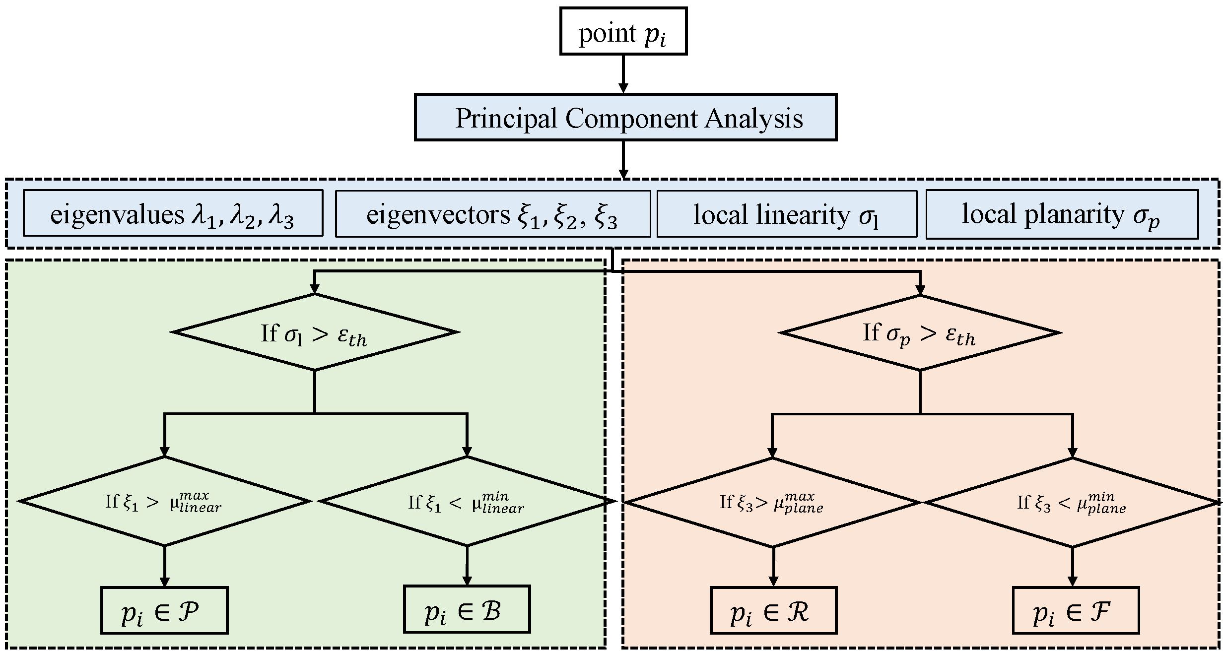
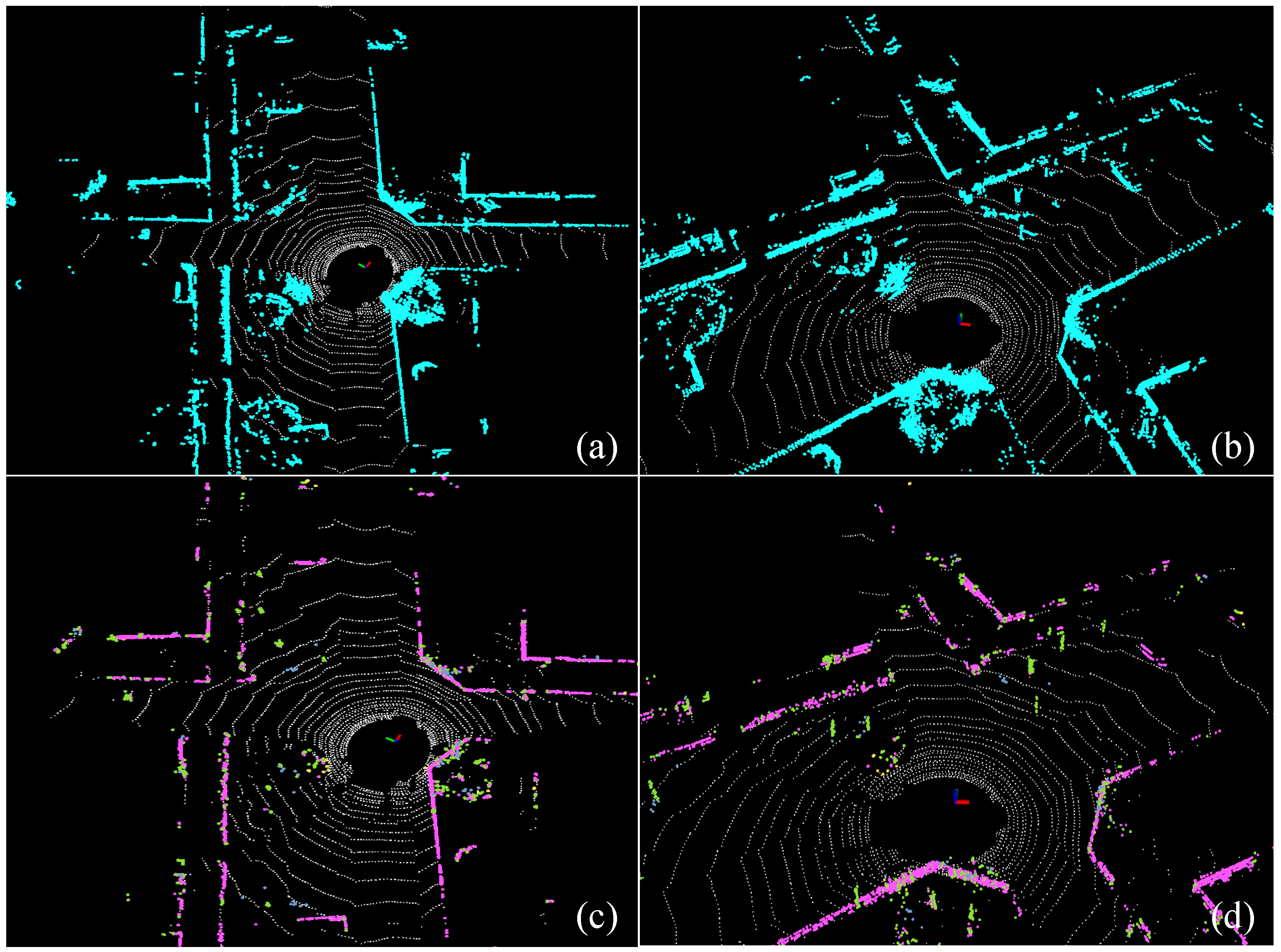
3.3. Multi-Category Feature Extraction Module

In this module, we use principal component analysis (PCA) technology to extract multi-category feature points, including pillar, beam, roof, and façade. Compared with traditional line and plane feature points, we extract more categories and are more accurate, which can ensure the close correlation between features.
We apply PCA to the non-ground point cloud to classify it into multiple feature categories based on the differences in direction vectors and normal vectors. This method effectively prevents the selection of discrete points and is somewhat universal for various types of LiDAR. First, the non-ground points are downsampled to a fixed number and added to the KD-tree. The point cloud and the nearest neighbors found via KD-tree search are input into the principal component analysis (PCA) module, where each point is classified based on its local attributes. Formally, for a point cloud p k i , the k nearest neighbors within a radius R are found using the KD-tree, and the mean p ¯ and covariance matrix σ are computed, which can be expressed as
p ¯ = 1 n i = 1 n p i k
σ = 1 n i n ( p k i p ¯ ) ( p k i p ¯ ) T
Here, n represents the number of neighboring points searched. Next, we perform singular value decomposition (SVD) on the covariance matrix to obtain the eigenvalues λ 1 , λ 2 , λ 3 ( λ 1 > λ 2 > λ 3 ) and their corresponding eigenvectors. These features can be differentiated using the eigenvectors of the covariance matrix. The largest eigenvector, denoted as l, represents the main distribution direction of the neighborhood point cloud, while the smallest eigenvector, denoted as n, represents the normal vector of the neighborhood point cloud. Discrete points that do not have enough neighboring points will be filtered out. By utilizing the eigenvalues of the covariance matrix, we can compute the local linearity σ l and planarity σ p of the point cloud, as expressed by
σ l = λ 1 λ 2 λ 1 ,   σ p = λ 2 λ 3 λ 1
Based on these geometric attributes, the non-ground point cloud can be categorized into multiple feature categories, including facades F , roofs R , pillars P , and beams B . The specific classification procedure is illustrated in Figure 2. In particular, if the local linearity exceeds a predefined threshold ε t h , the point is classified as a line feature point. Conversely, if the local planarity exceeds the threshold ε t h , the point is categorized as a plane feature point. Furthermore, if the z value of the main direction of the line point is greater than the threshold μ l i n e a r m a x , then the point belongs to P . If the main direction threshold of the line point is less than μ l i n e a r m i n , then the point belongs to B . If the z value of the main direction of the surface point is greater than a certain value μ p l a n e m a x , then the point belongs to R ; if the z value of the main direction of the surface point is less than a certain value μ p l a n e m i n , then the point belongs to F . Here, ε t h is set to 0.62, μ l i n e a r m a x is set to 0.94, μ l i n e a r m i n is set to 0.17, μ p l a n e m a x is set to 0.98, and μ p l a n e m i n is set to 0.34, which is consistent with MULLS [11].
Using multi-category feature extraction, we obtain line features that include P and B , and plane features that encompass F , R , and G .
Figure 3 illustrates the feature extraction results of the proposed method. Figure 3a,b show the ground and non-ground segmentation results in two different scenes. Figure 3c,d present the subsequent multi-category feature extraction results from the non-ground points, where pillars are shown in green, facades in magenta, beams in yellow, and roofs in light blue.
As shown in Figure 4, the green points represent the line features extracted by our method and LIO-SAM, while the purple points indicate the plane features. Figure 4a shows the visual image of the scene, while Figure 4b,c present the feature extraction results of our method and LIO-SAM, respectively. From the red, yellow, and green boxes, it can be observed that our method is able to extract more accurate line features (green points) even under such sparse conditions, whereas LIO-SAM incorrectly classifies the line structures within the boxes as plane features (purple points). In particular, in the yellow box, our method extracts only the points on the tree trunk as line features. In contrast, LIO-SAM classifies the entire tree, including branches and leaves, as plane features. It is important to note that branches and leaves usually lack stable geometric structure and are often regarded as noise. This indicates that our method demonstrates stronger robustness and better feature discrimination in such noisy environments.

3.4. Two-Stage Feature Correspondence Selection Module

Unlike well-known methods that directly use all associated feature correspondences for pose estimation, our feature correspondence selection focuses on eliminating incorrect correspondences and selecting a subset of the correct ones that contribute most significantly to pose estimation. In fact, different correspondences impose varying levels of constraint on the pose. Therefore, instead of treating all correspondences equally, we actively evaluate the contribution of each correspondence and prioritize those with richer geometric information and stronger constraint effectiveness. This method enhances both the accuracy and efficiency of the system by avoiding the adverse impact of redundant or weak correspondences. To this end, we propose a coarse-to-fine two-stage feature correspondence selection method.
Feature correspondence selection consists of three steps. First, feature correspondences are constructed based on point-to-line and point-to-plane geometric relationships. Second, incorrect correspondences are rejected by evaluating the local geometric consistency of the features. Finally, a greedy selection strategy is employed to extract a subset of correspondences that contribute most significantly to pose estimation.
Firstly, to establish the correspondence between the features { P , B , F , R , G } of the current frame and the local feature map, we use the KD-tree nearest neighbor search to identify the features of the same category and determine the feature correspondence. For line features (such as B   and   P ) in the current frame, when the largest eigenvalue of the covariance matrix of the point set within the search area is much greater than the second-largest and smallest eigenvalues, it indicates that the line feature search is correct. Subsequently, the two closest points p 1 and p 2 are found in the local line map, as is shown in Figure 5, and the line-to-line residual can be expressed as
L c i ( T ^ c ) = ( T ^ c p l i p M α ) × ( T ^ c p l i p M β ) p M α p M β
Here, T ^ c represents the pose to be estimated and × denotes the cross product.
Similarly, for plane feature points (such as F , R , and G ) in the current frame, when the smallest eigenvalue of the covariance matrix within the search region is much smaller than the largest and second-largest eigenvalues, it indicates that the plane feature search is correct. It is worth noting that the eigenvector corresponding to the smallest eigenvalue of the covariance matrix represents the normal vector of the search region. Subsequently, as is shown in Figure 6, the plane-to-plane geometric residual can be expressed as
L p i ( T ^ c ) = ( T ^ c p p i p ¯ j ) · n j
In this equation, p ¯ j represents the mean of the neighboring points, and n j is the normal vector of the plane formed by the neighboring points.
Secondly, we propose a feature selection method based on local geometric consistency to reject incorrect correspondences. This method compares the local geometric properties between feature points in the current frame and those in the local map. As shown in Figure 7a, v l i denotes the direction vector of a feature point in the current frame obtained using PCA, while v m i represents the direction vector estimated from neighboring points in the local map. The value cos θ l between the two normalized vectors is used to evaluate their consistency. A correct feature correspondence can be represented as
cos θ l i = v l i · v m i v l i · v m i > γ l
Similarly, as shown in Figure 7b, n l i denotes the normal vector of a feature point in the current frame obtained using PCA, while n m i represents the normal vector estimated from neighboring points in the local map. The value cos θ p between the two normalized vectors is used to evaluate their consistency. A correct feature correspondence can be represented as
cos θ p i = n l i · n m i n l i · n m i > γ p
Based on practical engineering experience, the value of γ l is set to 0.3 and the value of γ p is set to 0.3. Through the above process, the correct set of feature correspondences M can be obtained.
Thirdly, a greedy feature selection method is employed to extract a subset of correspondences that contribute the most to pose estimation. Specifically, the feature subset is selected through the following steps:
Step 1: Randomly sample n s feature correspondences from the full correspondence set, with the total computation time limited to t max milliseconds.
Step 2: For each sampled correspondence, compute its information matrix Λ i , defined as
Λ i = J i Σ i 1 J i
where J i is the Jacobian matrix and Σ i is the measurement noise covariance.
Step 3: Iterate over all candidates and identify the correspondence whose information matrix maximizes the objective function log det ( A + Λ i ) , where A denotes the accumulated information matrix of the selected subset.
Step 4: Add the correspondence with the highest contribution Λ i to the selected subset and update the matrix A:
A = A + Λ i
Step 5: Repeat Steps 1–4 until 80% of the desired number of correspondences have been selected.
After greedy feature correspondence selection, a set of correct and highly contributive feature correspondences is identified and denoted as M .

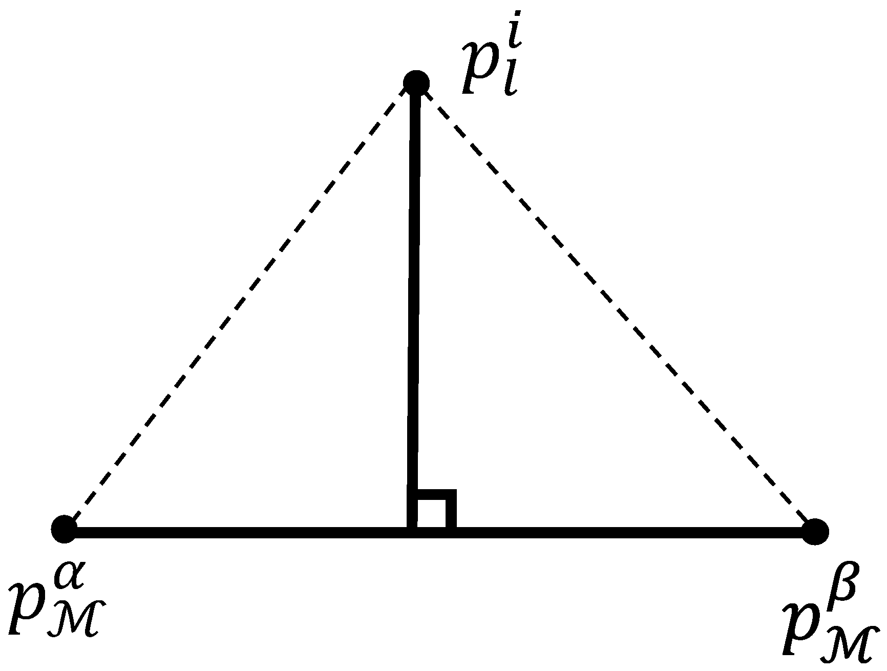
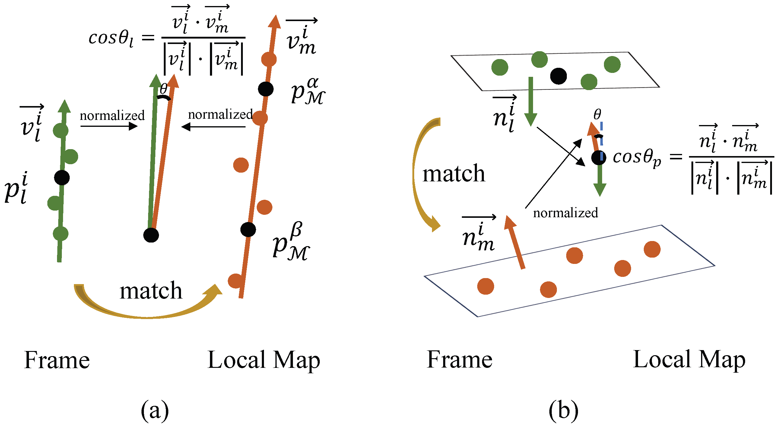
3.5. Adaptive Weighted Feature Matching Module

In this subsection, an adaptive weighted feature matching algorithm is employed to improve the accuracy of pose estimation. This method simultaneously considers both the distance of the feature constraints and the angular difference of local geometric properties, ensuring that correspondences with stronger geometric consistency are assigned higher weights.
The weight of line feature correspondence is denoted as ρ l i , is defined as
ρ l i = 1 0.9 · L c i ( T ^ c ) τ · cos θ l i
Based on practical engineering experience, the adjustment factor τ is set to 6. Similarly, the weight of plane feature correspondence, denoted as ρ p i , is defined as
ρ p i = 1 0.9 · L p i ( T ^ c ) O p p i · cos θ p i
Subsequently, the geometric residuals, which are calculated based on the selected line and plane feature correspondences, are used to estimate the pose transformation of the current frame relative to the initial coordinate system by solving an optimization problem. Essentially, the odometry problem is formulated as the minimization of these residuals to obtain the optimal pose:
arg min T ^ c i ( ρ l i L l i ( T ^ c ) 2 + ρ p i L p i ( T ^ c ) 2 )
We solve the above nonlinear optimization problem using the Gauss–Newton iteration to obtain the estimated pose T ^ c . Subsequently, the current frame’s point cloud is transformed into the local map coordinate system using the pose T ^ c , and the pose along with the current multi-class feature point cloud is stored, forming a pose library and a multi-class feature point cloud library. When the next frame arrives, the prior pose is used to search for the closest pose in the pose library. The corresponding multi-class feature point cloud of the closest pose is then accumulated to form the local feature point cloud map for the next frame.

3.6. Factor Graph Optimization Module

If the relative position Δ t and relative rotation Δ r between the current frame and the previous keyframe exceed a certain threshold, the current frame is selected as a keyframe. We construct a multi-keyframe factor graph optimization based on a sliding window to refine the keyframe poses. Within the factor graph framework, the keyframe pose at time t k can be represented as a state vector that includes position, velocity, and IMU gyro and accelerometer biases. This can be expressed as follows:
x k = [ R k T , p k T , v k T , b k g , b k a ] T
Here, R and p form the transformation T = [ R , p ] from the keyframe to the initial coordinate system, where the velocity, gyroscope bias, and accelerometer bias represent the current state of the vehicle. In the factor graph optimization, the set of states to be estimated can be expressed as x n = { x 1 , x 2 , , x i } . The refined pose transformation set can be obtained by solving a maximum a posteriori estimation problem or minimizing the negative log-likelihood, which can be expressed as follows:
x ^ n = arg min x n r 0 Σ 0 2 + k n r k I Σ I 2 + k n i r k i L Σ L 2 + k n r k Loop Σ Loop 2
where r 0 represents the prior factor, and Σ 0 denotes the prior covariance. The residual term r I and covariance Σ I represent the IMU pre-integration factor, while r L and covariance Σ L correspond to the multi-dimensional feature matching factor. r l o o p and Σ l o o p represent the loop closure factor and its covariance. Once a new keyframe arrives, it will be inserted into the factor graph, and incremental optimization will be performed within the fixed sliding window, with old keyframes being marginalized. The factor graph optimization model is shown in Figure 8.

3.6.1. IMU Pre-Integration Factor

For two adjacent keyframe times t k and t k + 1 , the IMU pre-integration residual r I can be expressed as follows:
r I z ^ I , x b ( k ) w , x b ( k + 1 ) w = r p r v r q r b a r b g = R b ( k ) w T p b ( k + 1 ) w p b ( k ) w v b ( k ) w Δ t + 1 2 g w Δ t 2 Δ p b ( k + 1 ) b ( k ) R b ( k ) w T v b ( k + 1 ) w v b ( k ) w + g w Δ t Δ v b ( k + 1 ) b ( k ) 2 Δ q b ( k + 1 ) b ( k ) 1 q w b ( k ) q b ( k + 1 ) w b a ( k + 1 ) b a ( k ) b g ( k + 1 ) b g ( k )
where ω ˜ b and a b represent the angular velocity and acceleration measured in the body frame, respectively; ω b and a w represent the true angular velocity and acceleration; b g and b a represent the biases of the gyroscope and accelerometer, respectively; n g and n a represent the noise of the gyroscope and accelerometer; g r is the gravity vector in the world frame; and R b is the rotation matrix from the world frame to the body frame. Where Δ R i j is the relative rotation between the frames, and Δ v i j and Δ p i j represent the increments in velocity and position, respectively. These increments are not related to true physical changes, but rather correspond to the pre-integrated IMU measurements. The exponential map Exp ( · ) is used for rotations in the special orthogonal group SO(3).

3.6.2. Multi-Category Feature Matching Factor

The multi-category feature matching factor of the LiDAR is created based on the selected keyframes, with the relative pose transformation T ^ b ( k + 1 ) b ( k ) between two adjacent keyframes serving as the inter-frame constraint. This can be expressed as follows:
T ^ b ( k + 1 ) b ( k ) = ( T l ( k ) w ) 1 T l ( k + 1 ) w
T ^ b ( k + 1 ) w = T ^ b ( k ) w T ^ b ( k + 1 ) b ( k )
The residual of the multi-category LiDAR point cloud matching factor can be expressed as
r L z L , x b ( k ) w , x b ( k + 1 ) w = ln ( ( R b ( k + 1 ) w ) 1 R b ( k ) w R ^ b ( k + 1 ) b ( k ) ) ( R b ( k + 1 ) w ) 1 ( R b ( k ) w t ^ b ( k + 1 ) b ( k ) + t b ( k ) w t b ( k + 1 ) w )
where ln ( · ) represents the logarithmic map that converts the rotation matrix into its vector form.

3.6.3. Loop Factor

Similar to LIO-SAM, due to the accumulation of odometry errors, the current keyframe pose T c w is not accurate. Loop closure compensation can provide a corrected keyframe pose T c w , which is expressed as
T c w = T w w T c w
where the relative pose transformation between the current keyframe and the best loop-closure frame, obtained through the ICP registration algorithm, can be denoted as T w w .
Based on the corrected T c w , the relative pose transformation T l w with respect to the loop closure keyframe pose T l o o p w is used as a constraint between the loop closure frames, forming the loop closure factor, which can be expressed as
r c L o o p = ( T l o o p w ) 1 T c w
Finally, the factor graph optimization, integrating the IMU pre-integration factor, multi-class point cloud feature matching factor, and loop closure factor, can further enhance the accuracy of front-end point cloud feature matching.

4. Experiments

In this section, a series of experiments are conducted to validate the effectiveness of the proposed algorithm. We evaluate and compare performance on two public datasets, M2DGR [29] and KITTI [30], as well as our self-recorded dataset. The absolute trajectory error (ATE) is used as the primary metric to assess the performance of all SLAM algorithms. All experiments are carried out on a PC equipped with an Intel i7 CPU and 16 GB of RAM, running the robot operating system (ROS) on Ubuntu 20.04.

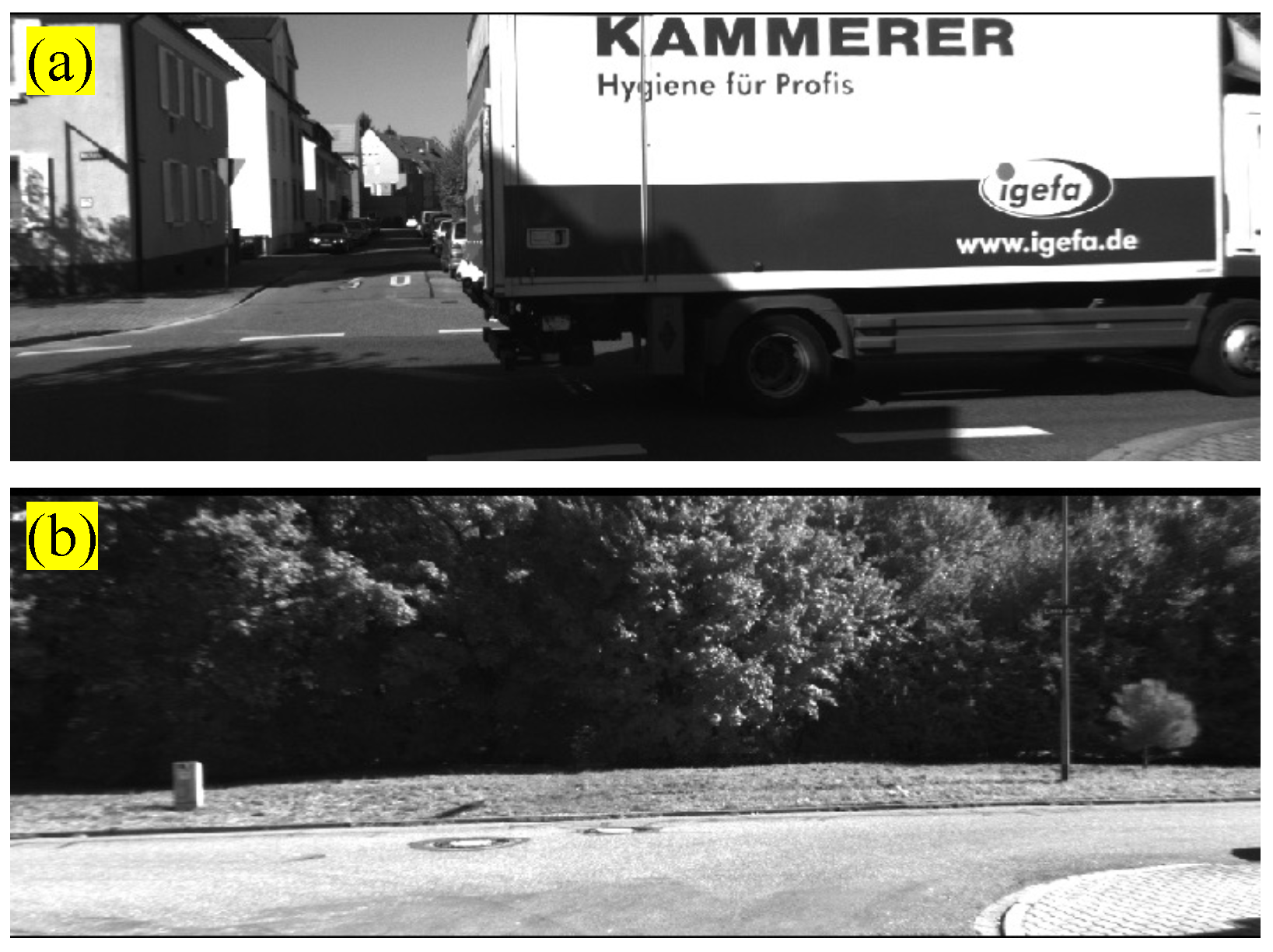
4.1. Dataset Description

The M2DGR [29] dataset was collected using a Velodyne VLP-32C LiDAR operating at 10 Hz and a Handheld A9 IMU at 150 Hz. We selected four outdoor street sequences, namely street03, street04, street05, and street06, to evaluate the performance of our algorithm.
The KITTI [30] dataset consists of sequences captured in various outdoor environments, where the LiDAR point clouds were acquired using a Velodyne HDL-64E sensor. The ground truth trajectories were obtained from a high-precision GPS/INS system. We use sequences 05 and 07 from the KITTI dataset to assess the performance of our approach.

4.2. Performance Evaluation

For ease of comparison, we use different labels to denote variants with different innovations. MGF-LIO-I is based on the original LIO-SAM, with modifications to support greedy feature correspondences selection. MGF-LIO-II builds on MGF-LIO-I by introducing a greedy feature correspondence selection strategy. MGF-LIO further extends MGF-LIO-II by incorporating coarse correspondence filtering based on local attribute consistency along with an adaptive weighted matching method.
To evaluate the performance of our proposed methods on public datasets, we conducted detailed comparisons with A-LOAM, F-LOAM, and LIO-SAM. The evaluations were performed on the M2DGR dataset using the street03, street04, street05, and street06 sequences, and on the KITTI dataset using sequences 05 and 07. The comparative results are summarized in Table 1. Our methods achieved higher accuracy across both datasets compared to A-LOAM, F-LOAM, KISS-ICP [31], Light-LOAM, FAST-LIO2, Point-LIO [32], and LIO-SAM, with an average minimum trajectory error of 0.643 m.
This improvement is attributed to the proposed multi-category feature extraction method, which extracts richer and more informative point cloud features based on local PCA analysis, reducing the sparsity and randomness of feature points. In addition, the coarse-to-fine two-stage feature correspondence selection method helps reject incorrect feature correspondences and identify a more effective subset of features that significantly contribute to pose estimation. Point-LIO and FAST-LIO2 achieved better performance on street05 and street06. However, due to the lack of loop closure, they did not perform satisfactorily on KITTI05 and KITTI07. Figure 9 shows the trajectories generated by the ten methods across different sequences.

4.3. Ablation Experiments Comparison

We conducted ablation studies to evaluate the contribution of each component in the proposed method. Table 1 presents a comparison of localization accuracy between our method and LIO-SAM. Compared with LIO-SAM, MGF-LIO-I achieves higher accuracy across all six sequences. It is worth noting that MGF-LIO-I shares the same feature extraction module as LIO-SAM, with improvements applied only during the feature matching stage through a greedy feature selection strategy. This indicates that our proposed point-to-line feature-based active selection algorithm contributes to more accurate pose estimation. MGF-LIO further improves upon MGF-LIO-II by achieving the lowest average absolute trajectory error. This demonstrates the effectiveness of the proposed coarse correspondence filtering based on local geometric consistency and the adaptive weighted feature matching method. Figure 10 and Figure 11 provide a detailed comparison of the estimated trajectories from ten different methods against the ground truth on the KITTI05 and KITTI07 sequences. As shown in the zoomed-in views, the trajectory produced by our method, MGF-LIO, aligns more closely with the ground truth.

4.4. Time Efficiency Evaluation

As shown in Table 2, we compare the runtime of feature extraction and feature matching between our method and state-of-the-art approaches on the KITTI07 dataset. It can be observed that our method incurs higher computational cost in the feature extraction stage, mainly due to the PCA computation required for multi-category feature extraction. Overall, our method is approximately 10 ms slower than LIO-SAM. However, it still operates in real-time, with the total processing time well below the 100 ms limit imposed by a 10 Hz LiDAR. Moreover, our method achieves higher localization accuracy compared to LIO-SAM.

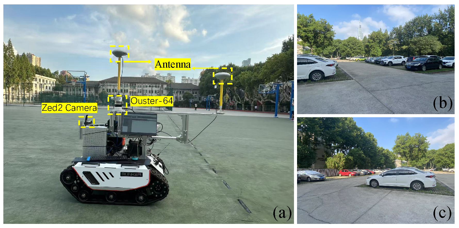
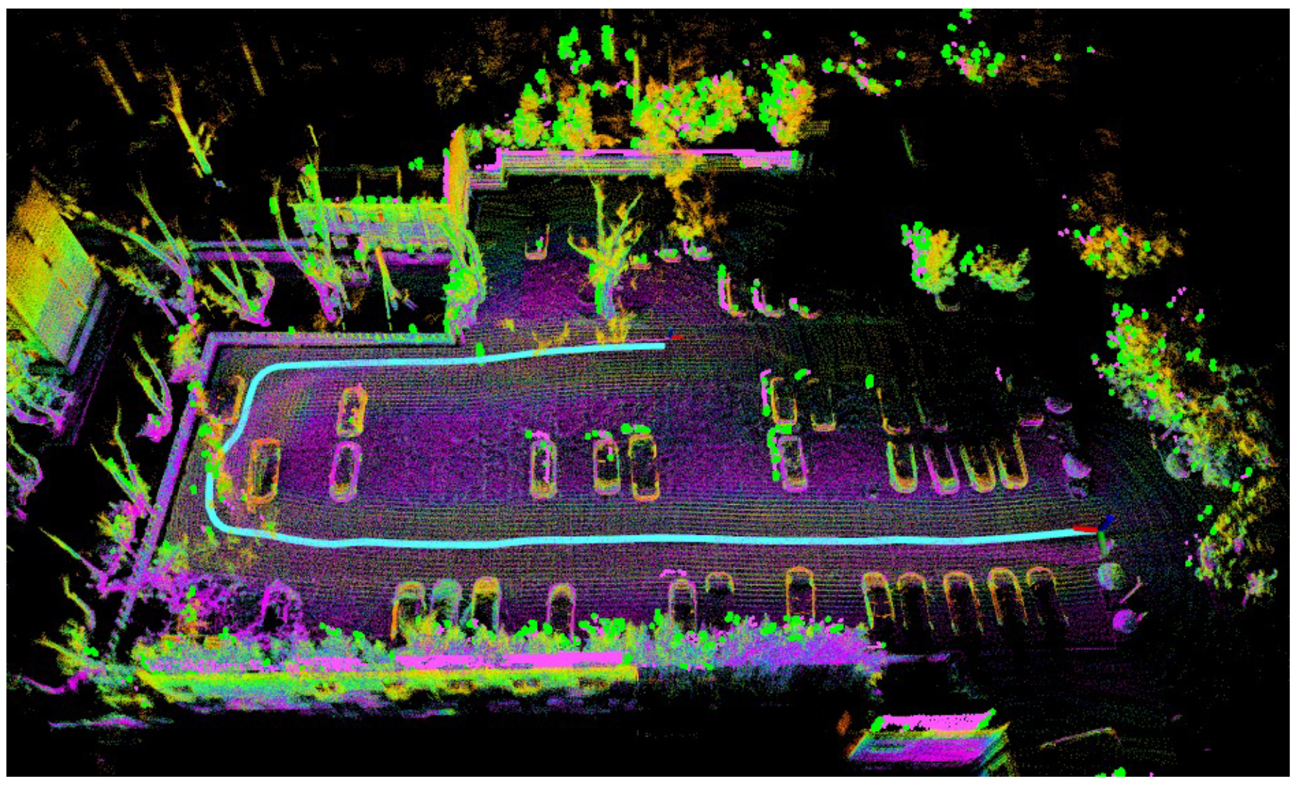
4.5. Campus Experiment

In this subsection, we validate our algorithm in a campus environment. As shown in Figure 12, our experimental platform is equipped with an Ouster 64-line LiDAR, an embedded IMU, and a GNSS receiver for ground-truth acquisition. Sensor data were collected in a parking lot. Table 3 presents the localization results in this environment, demonstrating that our method achieves higher accuracy compared to other approaches. The mapping result generated by our method is shown in Figure 13.

4.6. Limitation

However, our method still encounters certain limitations, particularly in highly dynamic environments and environments with sparse features. As illustrated in Figure 14a, due to the presence of strong geometric structures on moving vehicles, our multi-category feature extraction method inevitably selects features on these objects and establishes feature correspondences. Since large plane surfaces on vehicle bodies exhibit minimal geometric differences between consecutive frames and the local map, the coarse feature correspondence selection based on local geometric consistency fails to reject these dynamic feature matches. As a result, the resulting constraints will negatively affect the pose estimation during optimization. As shown in Figure 14b, in feature sparse scenes such as undergrowth or open areas, the proposed multi-category feature extraction method cannot obtain sufficient structured features from the environment. This leads to a lack of valid feature correspondences, which limits the effectiveness of pose estimation. Therefore, the method also faces performance degradation in scenes with low feature richness.

5. Conclusions

This paper presents a LiDAR inertial SLAM method based on multi-category feature extraction and selection. The proposed improvements focus primarily on the modules of feature extraction, feature correspondence selection, and feature matching. Through evaluations on public datasets and ablation studies, we demonstrate that the proposed method achieves higher accuracy than several state-of-the-art LiDAR and LiDAR inertial SLAM approaches. Specifically, the method enables the more accurate extraction of stable multi-category point cloud features. In addition, the proposed two-stage feature correspondence selection, consisting of coarse filtering followed by fine selection, effectively rejects incorrect matches and identifies the most contributive subset of features for pose estimation. This leads to improved overall accuracy. In future work, we aim to improve the computational efficiency of the multi-category feature extraction process and extend the method to dynamic environments. Identifying the relative constraint strength of different feature types in dynamic scenes may further enhance the overall performance of LiDAR inertial odometry.

Author Contributions

Conceptualization, N.L., Y.Y. and X.X.; methodology, N.L.; software, N.L., S.Z. and T.Y.; validation, Y.Y. and X.X.; formal analysis, N.L.; investigation, N.L.; resources, Y.Y., X.X. and N.L.; data curation, N.L.; writing—original draft preparation, N.L.; writing—review and editing, N.L.; supervision, Y.Y. and X.X. All authors have read and agreed to the published version of the manuscript.

Funding

This work was supported in part by the National Natural Science Foundation of China under Grants 52471358; in part by Jiangsu Provincial Department of Science and Technology under Grant BM2023013; in part by the Research Fund for Advanced Ocean Institute of Southeast University, Nantong under Grants KP202403; in part by the Zhishan Youth Scholar Program of Southeast University under Grant 2242024RCB0023.

Data Availability Statement

The original contributions presented in the study are included in the article; further inquiries can be directed to the corresponding author.

Conflicts of Interest

The authors declare no conflicts of interest.

References

  1. Gu, S.; Yao, S.; Yang, J.; Xu, C.; Kong, H. LiDAR-SGMOS: Semantics-guided moving object segmentation with 3D LiDAR. In Proceedings of the 2023 IEEE/RSJ International Conference on Intelligent Robots and Systems (IROS), Detroit, MI, USA, 1–5 October 2023; pp. 70–75. [Google Scholar]
  2. Parker, C.A.; Zhang, H. Cooperative decision-making in decentralized multiple-robot systems: The best-of-n problem. IEEE/ASME Trans. Mechatron. 2009, 14, 240–251. [Google Scholar] [CrossRef]
  3. Alterovitz, R.; Koenig, S.; Likhachev, M. Robot planning in the real world: Research challenges and opportunities. Ai Mag. 2016, 37, 76–84. [Google Scholar] [CrossRef]
  4. Zhang, J.; Singh, S. LOAM: Lidar odometry and mapping in real-time. In Proceedings of the Robotics: Science and Systems, Berkeley, CA, USA, 12–16 July 2014; Volume 2, pp. 1–9. [Google Scholar]
  5. Zhang, J.; Yao, Y.; Deng, B. Fast and robust iterative closest point. IEEE Trans. Pattern Anal. Mach. Intell. 2021, 44, 3450–3466. [Google Scholar] [CrossRef] [PubMed]
  6. Shan, T.; Englot, B. Lego-loam: Lightweight and ground-optimized lidar odometry and mapping on variable terrain. In Proceedings of the 2018 IEEE/RSJ International Conference on Intelligent Robots and Systems (IROS), Madrid, Spain, 1–5 October 2018; pp. 4758–4765. [Google Scholar]
  7. Bundy, A.; Wallen, L. Breadth-first search. In Catalogue of Artificial Intelligence Tools; Springer: Berlin/Heidelberg, Germany, 1984; p. 13. [Google Scholar]
  8. Abdi, H.; Williams, L.J. Principal component analysis. Wiley Interdiscip. Rev. Comput. Stat. 2010, 2, 433–459. [Google Scholar] [CrossRef]
  9. Guo, S.; Rong, Z.; Wang, S.; Wu, Y. A LiDAR SLAM with PCA-based feature extraction and two-stage matching. IEEE Trans. Instrum. Meas. 2022, 71, 1–11. [Google Scholar] [CrossRef]
  10. Chang, D.; Zhang, R.; Huang, S.; Hu, M.; Ding, R.; Qin, X. WiCRF: Weighted bimodal constrained LiDAR odometry and mapping with robust features. IEEE Robot. Autom. Lett. 2022, 8, 1423–1430. [Google Scholar] [CrossRef]
  11. Pan, Y.; Xiao, P.; He, Y.; Shao, Z.; Li, Z. MULLS: Versatile LiDAR SLAM via multi-metric linear least square. In Proceedings of the 2021 IEEE International Conference on Robotics and Automation (ICRA), Xi’an, China, 30 May–5 June 2021; pp. 11633–11640. [Google Scholar]
  12. Liang, S.; Cao, Z.; Guan, P.; Wang, C.; Yu, J.; Wang, S. A novel sparse geometric 3-d lidar odometry approach. IEEE Syst. J. 2020, 15, 1390–1400. [Google Scholar] [CrossRef]
  13. Su, Y.; Zhang, S.; Zhang, C.; Wu, Y. A 3D Lidar Odometry and Mapping Method Based on Clustering-Directed Feature Point. IEEE Trans. Veh. Technol. 2024, 73, 18391–18401. [Google Scholar] [CrossRef]
  14. Li, W.; Hu, Y.; Han, Y.; Li, X. Kfs-lio: Key-feature selection for lightweight lidar inertial odometry. In Proceedings of the 2021 IEEE International Conference on Robotics and Automation (ICRA), Xi’an, China, 30 May–5 June 2021; pp. 5042–5048. [Google Scholar]
  15. Sharp, I.; Yu, K.; Guo, Y.J. GDOP analysis for positioning system design. IEEE Trans. Veh. Technol. 2009, 58, 3371–3382. [Google Scholar] [CrossRef]
  16. Jiao, J.; Zhu, Y.; Ye, H.; Huang, H.; Yun, P.; Jiang, L.; Wang, L.; Liu, M. Greedy-based feature selection for efficient lidar slam. In Proceedings of the 2021 IEEE International Conference on Robotics and Automation (ICRA), Xi’an, China, 30 May–5 June 2021; pp. 5222–5228. [Google Scholar]
  17. Shan, T.; Englot, B.; Meyers, D.; Wang, W.; Ratti, C.; Rus, D. Lio-sam: Tightly-coupled lidar inertial odometry via smoothing and mapping. In Proceedings of the 2020 IEEE/RSJ International Conference on Intelligent Robots and Systems (IROS), Las Vegas, NV, USA, 25–29 October 2020; pp. 5135–5142. [Google Scholar]
  18. Zhao, S.; Fang, Z.; Li, H.; Scherer, S. A robust laser-inertial odometry and mapping method for large-scale highway environments. In Proceedings of the 2019 IEEE/RSJ International Conference on Intelligent Robots and Systems (IROS), Macau, China, 3–8 November 2019; pp. 1285–1292. [Google Scholar]
  19. Qin, C.; Ye, H.; Pranata, C.E.; Han, J.; Zhang, S.; Liu, M. Lins: A lidar-inertial state estimator for robust and efficient navigation. In Proceedings of the 2020 IEEE International Conference on Robotics and Automation (ICRA), Paris, France, 31 May–31 August 2020; pp. 8899–8906. [Google Scholar]
  20. Júnior, G.P.C.; Rezende, A.M.; Miranda, V.R.; Fernandes, R.; Azpúrua, H.; Neto, A.A.; Pessin, G.; Freitas, G.M. EKF-LOAM: An adaptive fusion of LiDAR SLAM with wheel odometry and inertial data for confined spaces with few geometric features. IEEE Trans. Autom. Sci. Eng. 2022, 19, 1458–1471. [Google Scholar] [CrossRef]
  21. Xu, W.; Zhang, F. Fast-lio: A fast, robust lidar-inertial odometry package by tightly-coupled iterated kalman filter. IEEE Robot. Autom. Lett. 2021, 6, 3317–3324. [Google Scholar] [CrossRef]
  22. Xu, W.; Cai, Y.; He, D.; Lin, J.; Zhang, F. Fast-lio2: Fast direct lidar-inertial odometry. IEEE Trans. Robot. 2022, 38, 2053–2073. [Google Scholar] [CrossRef]
  23. Zhang, Y.; Tian, Y.; Wang, W.; Yang, G.; Li, Z.; Jing, F.; Tan, M. RI-LIO: Reflectivity image assisted tightly-coupled LiDAR-inertial odometry. IEEE Robot. Autom. Lett. 2023, 8, 1802–1809. [Google Scholar] [CrossRef]
  24. Li, K.; Li, M.; Hanebeck, U.D. Towards high-performance solid-state-lidar-inertial odometry and mapping. IEEE Robot. Autom. Lett. 2021, 6, 5167–5174. [Google Scholar] [CrossRef]
  25. Nguyen, T.M.; Duberg, D.; Jensfelt, P.; Yuan, S.; Xie, L. Slict: Multi-input multi-scale surfel-based lidar-inertial continuous-time odometry and mapping. IEEE Robot. Autom. Lett. 2023, 8, 2102–2109. [Google Scholar] [CrossRef]
  26. Yi, S.; Lyu, Y.; Hua, L.; Pan, Q.; Zhao, C. Light-LOAM: A lightweight lidar odometry and mapping based on graph-matching. IEEE Robot. Autom. Lett. 2024, 9, 3219–3226. [Google Scholar] [CrossRef]
  27. Guo, H.; Zhu, J.; Chen, Y. E-LOAM: LiDAR odometry and mapping with expanded local structural information. IEEE Trans. Intell. Veh. 2022, 8, 1911–1921. [Google Scholar] [CrossRef]
  28. Lin, Y.K.; Lin, W.C.; Wang, C.C. K-closest points and maximum clique pruning for efficient and effective 3-d laser scan matching. IEEE Robot. Autom. Lett. 2022, 7, 1471–1477. [Google Scholar] [CrossRef]
  29. Yin, J.; Li, A.; Li, T.; Yu, W.; Zou, D. M2dgr: A multi-sensor and multi-scenario slam dataset for ground robots. IEEE Robot. Autom. Lett. 2021, 7, 2266–2273. [Google Scholar] [CrossRef]
  30. Geiger, A.; Lenz, P.; Urtasun, R. Are we ready for autonomous driving? the kitti vision benchmark suite. In Proceedings of the 2012 IEEE Conference on Computer Vision and Pattern Recognition, Providence, RI, USA, 16–21 June 2012; pp. 3354–3361. [Google Scholar]
  31. Vizzo, I.; Guadagnino, T.; Mersch, B.; Wiesmann, L.; Behley, J.; Stachniss, C. Kiss-icp: In defense of point-to-point icp–simple, accurate, and robust registration if done the right way. IEEE Robot. Autom. Lett. 2023, 8, 1029–1036. [Google Scholar] [CrossRef]
  32. He, D.; Xu, W.; Chen, N.; Kong, F.; Yuan, C.; Zhang, F. Point-LIO: Robust high-bandwidth light detection and ranging inertial odometry. Adv. Intell. Syst. 2023, 5, 2200459. [Google Scholar] [CrossRef]
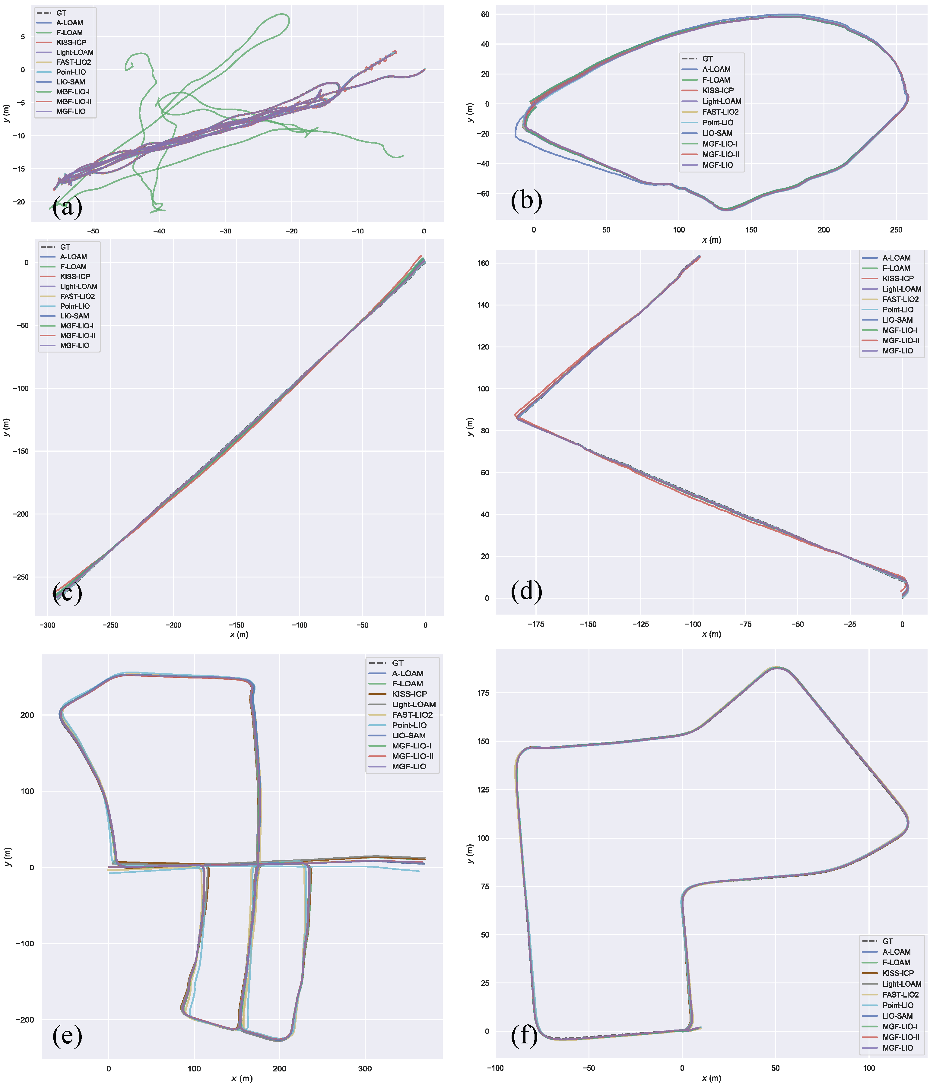
Figure 1. The overall framework of the proposed method consists of five components: a preprocessing module, a multi-category feature extraction module, a two-stage feature correspondence selection module, an adaptive weighted feature matching module, and a factor graph optimization module. The orange, blue, and green dashed boxes represent the three contributions that our method adds compared to LIO-SAM.
Remotesensing 17 02425 g001
Figure 2. Flowchart of multi-category feature extraction.
Remotesensing 17 02425 g002
Figure 3. The illustration of multi-category feature extraction results from different viewpoints of the same scene. Subfigures (a,b) show the segmented ground points (gray color) and non-ground points (cyan color). Subfigures (c,d) present the results of further multi-category feature extraction from the non-ground points, where pillars are shown in green color, facades in magenta color, beams in yellow color, and roofs in light blue color.
Remotesensing 17 02425 g003
Figure 4. Comparison of feature extraction results between LIO-SAM and the proposed method. (a) shows the visual image of a sparse scene, while (b,c) illustrate the feature extraction results of our method and LIO-SAM, respectively. The color scheme of the extracted feature points in our method is consistent with that in Figure 3. In LIO-SAM, edge features are shown in green, and planar features are shown in magenta. The red, yellow, and green boxes highlight the differences between our feature extraction results and those of LIO-SAM.
Remotesensing 17 02425 g004
Figure 5. Illustration of the point-to-line feature matching principle.
Remotesensing 17 02425 g005
Figure 6. Illustration of the point-to-plane feature matching principle.
Remotesensing 17 02425 g006
Figure 7. Schematic diagram of local geometric consistency to reject incorrect correspondences. (a) presents the schematic of directional consistency calculation for line feature matching, while (b) illustrates the schematic of directional consistency calculation for surface feature matching. The green and orange points represent points from the current frame and the map, respectively, and the black points denote virtual auxiliary points.
Remotesensing 17 02425 g007
Figure 8. Illustration of the factor graph optimization framework integrating LiDAR, inertial, and loop closure constraints.The flow blocks and arrows with a yellow background represent operations executed by the IMU; those with an orange background correspond to operations performed by the LiDAR; and those with a blue background indicate operations related to loop closure detection.
Remotesensing 17 02425 g008
Figure 9. Comparison of trajectory plots between the proposed method and other approaches on two datasets. Subfigures (af) illustrate the trajectory comparisons of various methods on the street03, street04, street05, street06, KITTI05, and KITTI07 sequences, respectively.
Remotesensing 17 02425 g009
Figure 10. A detailed comparison between the estimated trajectories of different methods and the ground truth over specific time intervals on the KITTI05 sequence.An enlarged view of the dashed box area is shown, as indicated by the arrow.
Remotesensing 17 02425 g010
Figure 11. A detailed comparison between the estimated trajectories of different methods and the ground truth over specific time intervals on the KITTI07 sequence.An enlarged view of the dashed box area is shown, as indicated by the arrow.
Remotesensing 17 02425 g011
Figure 12. Experimental platform and scene images of the campus test environment. (a) shows the experimental platform, with the LiDAR, camera, and antenna highlighted in the yellow dashed box. (b,c) present the real-world scenes from the campus test environment.
Remotesensing 17 02425 g012
Figure 13. Mapping results of the campus environment generated using our proposed method.
Remotesensing 17 02425 g013
Figure 14. Scenarios where the proposed method has limitations. (a) shows a scene with dynamic objects, while (b) depicts a scene with sparse features.
Remotesensing 17 02425 g014
Table 1. RMSE(m) comparison of ATE accuracy between the proposed method and other methods on two datasets.
Methodstreet03street04street05street06KITTI05KITTI07Avg.
A-LOAM0.1553.3910.7150.5403.2140.5331.425
F-LOAM15.6291.0802.3560.9253.6100.5904.032
KISS-ICP0.1661.5283.3532.1823.3270.6181.862
Light-LOAM0.1460.5201.2150.7423.4820.5281.106
FAST-LIO20.1820.4350.3640.3974.0311.4231.139
Point-LIO0.1860.5510.2980.3035.6061.1521.349
LIO-SAM0.1441.9241.7410.9131.3220.4661.085
MGF-LIO-I0.1411.8791.6780.7301.0560.4550.990
MGF-LIO-II0.1391.1490.7230.7490.8150.3800.659
MGF-LIO0.1411.0740.7180.5690.9870.3670.643
Table 2. Comparison of feature extraction and feature matching time efficiency (ms) between LIO-SAM and the proposed method.
MethodFeature ExtractionFeature MatchingTotal Time
LIO-SAM7.41638.20645.622
MGF-LIO37.26314.97852.241
Table 3. Comparison of ATE accuracy between the proposed method and other methods in a campus environment.
MethodA-LOAMF-LOAMLIO-SAMMGF-LIO-IMGF-LIO-IIMGF-LIO
Parking lot0.1830.1650.1580.1560.1530.151
Disclaimer/Publisher’s Note: The statements, opinions and data contained in all publications are solely those of the individual author(s) and contributor(s) and not of MDPI and/or the editor(s). MDPI and/or the editor(s) disclaim responsibility for any injury to people or property resulting from any ideas, methods, instructions or products referred to in the content.

