Measurement of Suspended Sediment Concentration at the Outlet of the Yellow River Canyon: Using Sentinel-2 Images and Machine Learning

Abstract

The remote sensing inversion of the Suspended Sediment Concentration (SSC) at the Yellow River estuary is crucial for regional sediment management and the advancement of monitoring techniques for highly turbid waters. Traditional in situ methods and low-resolution imagery are no longer sufficient for high-accuracy studies. Using SSC data from the Longmen Hydrological Station (2019–2020) and Sentinel-2 imagery, multiple models were compared, and the random forest regression model was selected for its superior performance. A non-parametric regression model was developed based on optimal band combinations to estimate the SSC in high-sediment rivers. Results show that the model achieved a high coefficient of determination (R² = 0.94) and met accuracy requirements considering the maximum SSC, MAPE, and RMSE. The B4, B7, B8A, and B9 bands are highly sensitive to high-concentration sediment rivers. SSC exhibited significant seasonal and spatial variation, peaking above 30,000 mg/L in summer (July–September) and dropping below 1000 mg/L in winter, with a positive correlation with discharge. Spatially, the SSC was higher in the gorge section than in the main channel during the flood season and higher near the banks than in the river center during the dry season. Overall, the random forest model outperformed traditional methods in SSC prediction for sediment-laden rivers.

1. Introduction

The Suspended Sediment Concentration (SSC) is one of the most critical water quality parameters in rivers, and sediment transport is an essential hydrological process [1]. The SSC in water affects a number of water’s optical properties, such as transparency, turbidity, and color [2]. In addition, the sediment content of the river greatly influences the balance of the river channel, and local sediment deposition causes problems such as river bed deformation [3]. The UNESCO-ISI Online Training Workshop on Sediment Transport Measurement and Monitoring highlighted the importance of measuring and monitoring sediment transport and managing and mitigating its negative effects [4].

The traditional SSC survey method measures point-by-point sampling with the ship on site, which is time-consuming and costly, and it is difficult to monitor a large area of water for a long time [5]. In this sense, remote sensing technology possesses characteristics such as strong macroscopic viability and comprehensiveness, high comprehensive benefit, a large amount of information, a rapid update cycle, and a wide range of application fields. In addition, the realization of long-term earth observation and the monitoring of inaccessible areas also makes remote sensing a very promising technology. Therefore, remote sensing is valuable for quantifying the SSC in river systems [6].

The current SSC inversion is divided into parametric and non-parametric models. The parametric model is a mathematical and statistical model in which the uncertainty between the water body information and the remote sensing information is assumed to be a specific functional relationship. The model parameters are estimated by converting them into a multivariate linear function [7]. Cai et al. developed a linear model using the HaiYang-1C (HY-1C) satellite to retrieve the SSC in the Zhoushan offshore waters [8]. Zhang and Guo constructed a single-band empirical statistical model and a band combination empirical statistical model in the Zhoushan offshore area using GaoFen-1 (GF-1) data, analyzed the correlation coefficients between various models, and verified their accuracy. They indicated that the inversion accuracy is higher in the quadratic model based on the combination of red and green bands (Band 3/Band 2) [9]. The parametric model is intuitive, easy to understand, and has many applications. However, it usually requires the sample population to meet specific distribution characteristics (such as normal distribution), and the wide-spread spatiotemporal autocorrelation of water parameters cannot meet the assumptions [10]. Therefore, this assumption has theoretical flaws, which lower the model’s prediction accuracy and generalization performance [11]. Non-parametric models make no assumptions about the overall distribution of samples; they are a statistical analysis method for directly analyzing samples. They have a wide range of applications and high reliability, so they are favored by many scholars. The relationship between ocean suspended matter and remote sensing image was established via Support Vector Machine (SVM) [12]. Additionally, Extreme Learning Machines (ELMs) were used in neural network and Landsat satellite images to reverse the SSC in Missouri and Mississippi rivers [13]. In contrast, machine learning also has some problems [14]. For example, the performance of machine learning methods is mainly dependent on a large number of training samples, which are usually difficult to obtain in real-world scenarios [15]. In addition, deeper networks result in high computational costs and overfitting, and the issue of balancing network depth and computational efficiency must be addressed [16].

The Random Forest (RF) model is a machine learning method based on classification trees [17]. It is flexible, robust, practical, efficient, and can be used for regression, clustering, classification, prediction, and other analyses. Since the model has obvious advantages in parameter optimization, variable sorting, subsequent variable analysis, and interpretation, it is ideally suited for simulating suspended sediment [18]. The SSC along the Missouri River was estimated by using the SVR and RF models, and it was found that the RF model performs better [19]. A new river turbidity measurement model based on RF was proposed, and excellent results were obtained, which proved the potential of RF in river detection [20].

Researchers have investigated the relationship between remote sensing reflectance data at visible and near-infrared wavelengths in the past few decades and the SSC, utilizing large rivers as the study area [21,22]. The current research still has some limitations. First, the sediment concentrations in large rivers are generally low and stable. For example, the Yangtze [18], the Missouri River [23], and the Mississippi River [13] are current research hotspots. These rivers have an average sediment concentration between 83 and 395 mg/L. However, there are relatively few studies on rivers with a high sediment concentration. Second, due to the limitations of the quality and availability of satellite images, many previous studies used low-resolution remote sensing image data to detect the long-time variation trend of river sediment (e.g., MODIS with a spatial resolution of 250–1000 m) [13,24,25]. However, when the river channel in the study area is narrow, the resolution of these images cannot adequately meet the research requirements.

The Yellow River, the mother river of the Chinese nation, is famous for its high sediment concentration. Its average sediment concentration is 1.44 × 10⁴ mg/L, and the fluctuation is huge, with a peak value of 7 × 10⁴ mg/L [26]. The problem of hanging rivers on the Earth’s surface in the downstream areas is becoming increasingly severe, and dam failure poses a serious risk to human life. The SSC of the Yellow River has become a vital factor affecting the ecological environment of the Yellow River Basin. Sediment control in the Yellow River is an urgent task. The Qin Jin Canyon of the Yellow River is located on the Loess Plateau, and a large amount of sediment is transported downstream yearly, which is the primary source of Yellow River sediment [27,28]. Hence, monitoring the concentration of suspended particulate matter at the outlet of the Yellow River Canyon is valuable for understanding the specific situation of Yellow River sediment, which is of great scientific interest. For the SSC study of the Yellow River, most current investigations focus on the estuary [29,30,31,32], while the middle reaches of the Yellow River, especially the mountainous areas, are seldom. This is detrimental to the ecological protection of the Yellow River Basin. In the past, this type of research has been hindered by the limitations of remote sensing image resolution. Sentinel-2 satellite images, with higher resolution, a shorter revisit period, and multiband, can effectively solve these problems [33,34,35].

The outlet of the Yellow River Canyon is selected as the study area to investigate the relationship between the SSC and remote sensing reflectance in high-sediment- concentration rivers. This study focuses on the SSC inversion and spatial distribution at the Yellow River Canyon outlet using Sentinel-2 satellite imaging, data on the daily average sediment content of the Yellow River, and a random forest model. The specific research objectives of this research are as follows:

(1)

Building a non-parametric inversion model, dividing the sample point into several types by attributes (season, hydrological situation), and finding the optimal inversion model through model checking.

(2)

Applying the optimal inversion model, performing remote sensing estimation of the SSC distribution in the study area, and analyzing the concentration of suspended sediment and its temporal and spatial variation in the water body in this region.

This study provides essential information for managing and utilizing water resources in the middle reaches of the Yellow River and other inland rivers, enrich the research in the field of rivers with high concentrations of sediment and filling the gaps the in the sediment monitoring of the reach of the Yellow River without monitoring stations. At the same time, this study can also be combined with traditional inversion methods to provide a new method for the remote sensing monitoring of river sediment concentration.

2. Materials and Methods

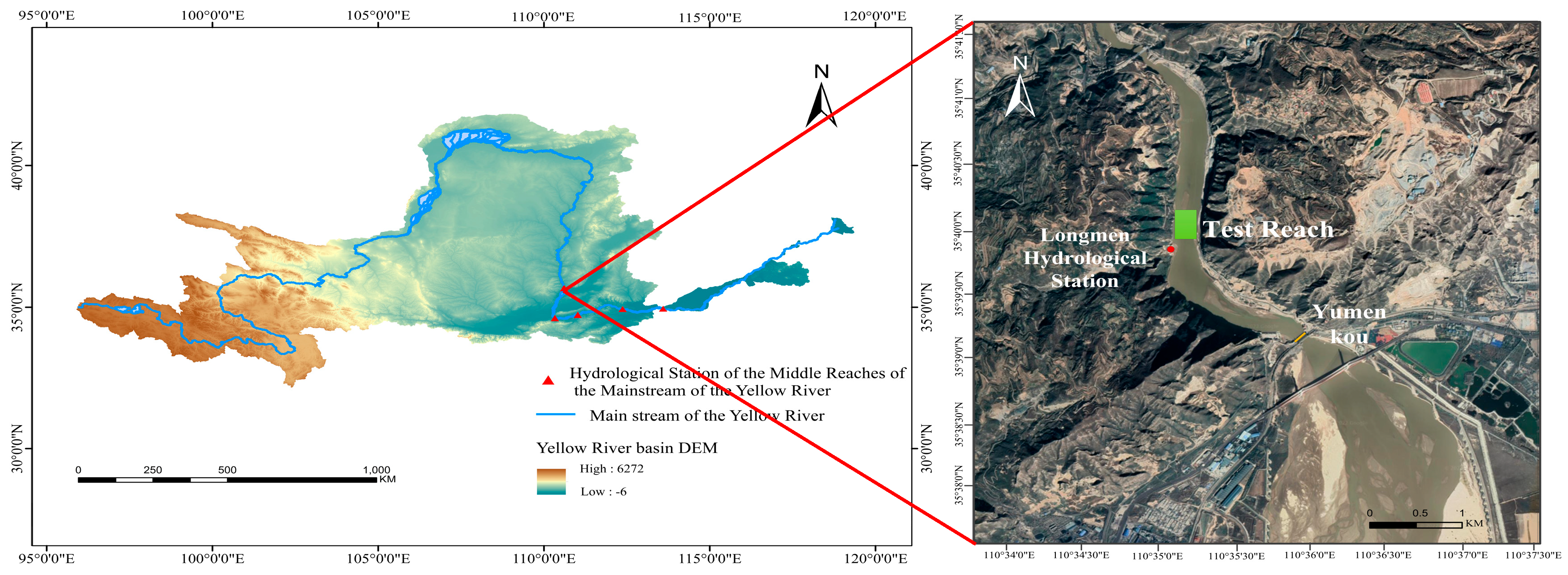
2.1. Case Study

The outlet of the Qin Jin Canyon of the Yellow River is YuMen Kou (110°60′ E, 35°65′ N), also known as Longmen. It is situated at the intersection of the Hejin City of Shanxi Province and the Hancheng City of Shaanxi Province. This region is a temperate continental climate [36]. More than 60% of the annual precipitation falls each year between June and September [37]. Upstream of YuMen Kou is Qinjin Canyon, located on the Loess Plateau. The soil is loose, the terrain is broken, the vegetation coverage is poor, the rainstorm is concentrated, and the rainfall is large, providing favorable conditions for transporting a large amount of sediment. This is the primary source of Yellow River sediment [38]. The downstream area of YuMen Kou is the Xiaobei mainstream (from YuMen Kou to Tongguan), which is a typical wandering river. In addition, the riverbed in this reach is seriously silted and uplifted, making it one of the most difficult reaches of the middle reaches of the Yellow River to control [39,40,41].

Longmen Hydrometric Station is located 1500 m upstream of YuMen Kou (110°35′ E, 35°40′ N). The test reach is approximately 400 m in length and 130 m in width. The bend and the checkpoint control the low-water channel and high-water section, as shown in Figure 1. Based on the data measured at the stations, from 1987 to 2020, the annual average runoff and sediment are 2.59 × 10⁹ m³ and 6.40 × 10⁸ t, respectively [26]. In this paper, the monitoring data of Longmen Station are used as the basis for inversion modeling and model verification.

2.2. Sentinel-2 MSI Data

The Sentinel-2 satellite is part of the Copernicus mission of the European Space Agency, which uses a constellation of satellites to observe Earth. Launched in June 2015 and March 2017, both satellites are equipped with an MSI (Multispectral Imaging System), covering 13 spectral bands and 290 km wide. The ground resolution is 10, 20, and 60 m (

Table A1. Spectral information for Sentinel-2 MSI.

Payload Band	Sentinel-2A		Sentinel-2B		Pixel Size(m)
	Central Wavelength (nm)	Spectral Width (nm, Half Height)	Central Wavelength (nm)	Spectral Width (nm, Half Height)
B1: Aerosols	442.7	21	442.2	21	60
B2: Blue	492.4	66	492.1	66	10
B3: Green	559.8	36	559.0	36	10
B4: Red	664.6	31	664.9	31	10
B5: Red Edge 1	704.1	15	703.8	16	20
B6: Red Edge 2	740.5	15	739.1	15	20
B7: Red Edge 3	782.8	20	779.7	20	20
B8: NIR	832.8	106	832.9	106	10
B8A: Red Edge 4	864.7	21	864.0	22	20
B9: Water Vapor	945.1	20	943.2	21	60
B11: SWIR 1	1613.7	91	1610.4	94	20
B12: SWIR 2	2202.4	175	2185.7	185	20

). The revisit period of one satellite is six days, and the two complement each other; hence, the revisit period is three days. It has various spatial resolutions, from visible and near-infrared to short-wave infrared.

Remote sensing images were obtained by querying the Google Earth Engine (GEE) for all Sentinel-2 Level-2A products from 2019 to 2020, which are provided by the European Space Agency (ESA), and processed using Sen2Cor for atmospheric correction, converting the data into surface reflectance. These products represent Bottom-of-Atmosphere (BOA) reflectance data that have been corrected for orthorectification, geometric distortions, and atmospheric effects. Existing studies have shown that the hyperspectral capability of Sentinel-2A, especially in the infrared band, enables the generation of effective sediment concentration models using reflectance data [42]. In order to reduce the influence of the solar scintillation effect, most of the image data adopt the midday period of sunny days, and multitemporal image data can reduce the influence of the solar scintillation effect on the fluctuation of reflectance. The following processing steps were applied to the 295 images retrieved:

(1)

Image filtering: Through visual interpretation and the band (QA60) of cloud mask information included with Sentinel-2 data, images in the study area that cannot be collected due to cloudy weather are filtered out. The cloud mask enables cloudy and cloud-free pixels to be identified. The pixel position is selected as far as possible in the middle of the river, and the adjacent pixels are reselected for the images exposed on land due to the reduction of water volume. Finally, 128 valid images were obtained.

(2)

Band reflectance information extraction: Because of the different spatial resolutions between MSI bands, each band is resampled to a 10m resolution before extracting the band reflectance. Due to the weak reflection signal of water bodies, the edge region of the water bodies is easily affected by the reflection of land pixels, making it difficult to represent the actual water surface. In order to eliminate the effect of land pixel reflection, considering the resolution of the resampled image and the width of the test river, the median filter template of 5 × 5 is selected [43]. Finally, in order to obtain the pure pixel, which is most likely to be the water body, the center of the river closest to the monitoring station is selected as the sampling point, and the image reflectivity after median filtering is extracted as the final reflectivity (Table S1).

2.3. Sediment Data

Longmen Hydrometric Station was established on the left bank outside YuMen Kou on June 14, 1934 (Longmen I). After several changes in September 1971, it moved to its current site (Mawang Miao II) (Figure 1). In 1974, the measurement method was changed from a gondola ropeway to a heavy lead fish electric ropeway and double-cable fixed hanging box, and this remains in use today. The daily average sediment concentration data at Longmen station from 2019 to 2020 was obtained through the Yellow River Conservancy Commission of the Ministry of Water Resources, and the process of sediment sampling and testing complies with the “Specification for Testing Suspended Sediment in Rivers GB T50159–2015” [44].

In accordance with national first-class station standards, suspended sediment transport rate, concentration, and particle size distribution should be measured through long-term, year-round observations. The first-class station should have no fewer than five sampling points, with sediment concentration and flow velocity measured at five different depths per point. The five-point method is used to calculate the daily average sediment concentration. Monitoring frequency should be increased during overlapping flood peaks, mismatched water-sediment peaks, or when sediment concentration varies significantly.

If strictly matched by the hour, the number of available samples will be significantly reduced, and it will be difficult to achieve complete synchronization with the instantaneous observations of hydrological stations. This paper collates the data of suspended sediment and the reflectance data of the spectral band of Sentinel-2 images on that day and uses the Dikson criterion to screen out outliers. Due to the excessive sediment concentration in the Yellow River, the inversion effect is not good as it directly uses the original sediment concentration data. In order to improve the accuracy of the model and ensure that the regression parameter estimator has good simulation effect, the natural logarithm of sediment concentration (expressed in terms of ln(SSC)) is applied to fit the reflectivity of each band [45].

2.4. Random Forest Model

2.4.1. Modeling Process

As shown in the table (Table S2), after a series of experiments, it was found that the band combination with a better inversion effect after linear fitting has a better inversion impact in random forest model regression, and the overall accuracy is higher than that of correlation, index fitting, and other indicators. The spectral reflectance of each band and ln(SSC) was fitted with the linear model, and the band combination with the better fitting effect was selected to participate in the construction of the random forest model. A total of 70% of the sample data is randomly selected from the sediment concentration dataset as the training sample set of the random forest regression model, and the remaining 30% is used as the testing sample set of the model.

The importance of each variable obtained by the random forest algorithm is determined. Variable importance refers to the contribution rate of the predictor variable to the prediction accuracy. The larger the value, the more important the variable is. Variable importance in the random forest model is relative and sums to 1. After the variables are sorted by importance, they must be screened to ensure that the model has fewer predictors and more accurate prediction effects. This not only simplifies the model but also facilitates the interpretation of subsequent models [46]. The variable selection adopts the backward elimination method; i.e., after sorting based on the importance, all variables are used as prediction parameters to construct a random forest algorithm. The model is then applied to estimate the test sample set, and its prediction accuracy is recorded. Finally, each variable is reduced individually, and the above process is repeated. The prediction accuracy of each model under different variable combinations is compared, and the combination with the highest accuracy is selected as the optimal variable group. The random forest algorithm model is then reconstructed to test the model’s prediction accuracy.

2.4.2. Model Checking

The primary evaluation indices of this paper are as follows: (1) the R² of the determination coefficient; (2) the mean-square error (MSE); and (3) the mean absolute percentage error (MAPE) as auxiliary [47], jointly assessing the accuracy of the model, comprehensively evaluating the prediction ability of all regression models, and testing the prediction results of regression models. The MSE is the mean value of the sum of the squared errors of the predicted data and the original data, and the MAPE is the percentage used to express model errors, which is relatively more intuitive and unaffected by the range of values of the original data. It is also more suitable for comparing different data (subsets). The calculation formula of each indicator is as follows:

$$R^2=1-{\displaystyle \frac{\sum _{i=1}^n{({\widehat{y}}_i-y_i)}^2}{\sum _{i=1}^n{({\overline{y}}_i-y_i)}^2}}$$

(1)

$$MSE={\displaystyle \frac{1}{n}}\sum _{i=1}^n{{\sum }_{i=1}^n({\widehat{y}}_i-y_i)}^2$$

(2)

$$MAPE={\displaystyle \frac{100\%}{n}}\sum _{i=1}^n\left|{\displaystyle \frac{{\widehat{y}}_i-y_i}{{\widehat{y}}_i}}\right|$$

(3)

where n is the total number of samples, ${\overline{y}}_i$ is the average value of the natural logarithm of the concentration of sediment in the dataset, $y_i$ is the natural logarithm of the concentration of sediment in the $i$ ($i$ = 1, 2, 3, ⋯, n) sample point in the dataset, and ${\widehat{y}}_i$ is the natural logarithm of the concentration of sediment in the $i$ ($i$ = 1, 2, 3, ⋯, n) sample point predicted by the prediction model. The higher the R² and the lower the MSE and MAPE, the better the model fitting effect and the higher the inversion precision.

3. Results

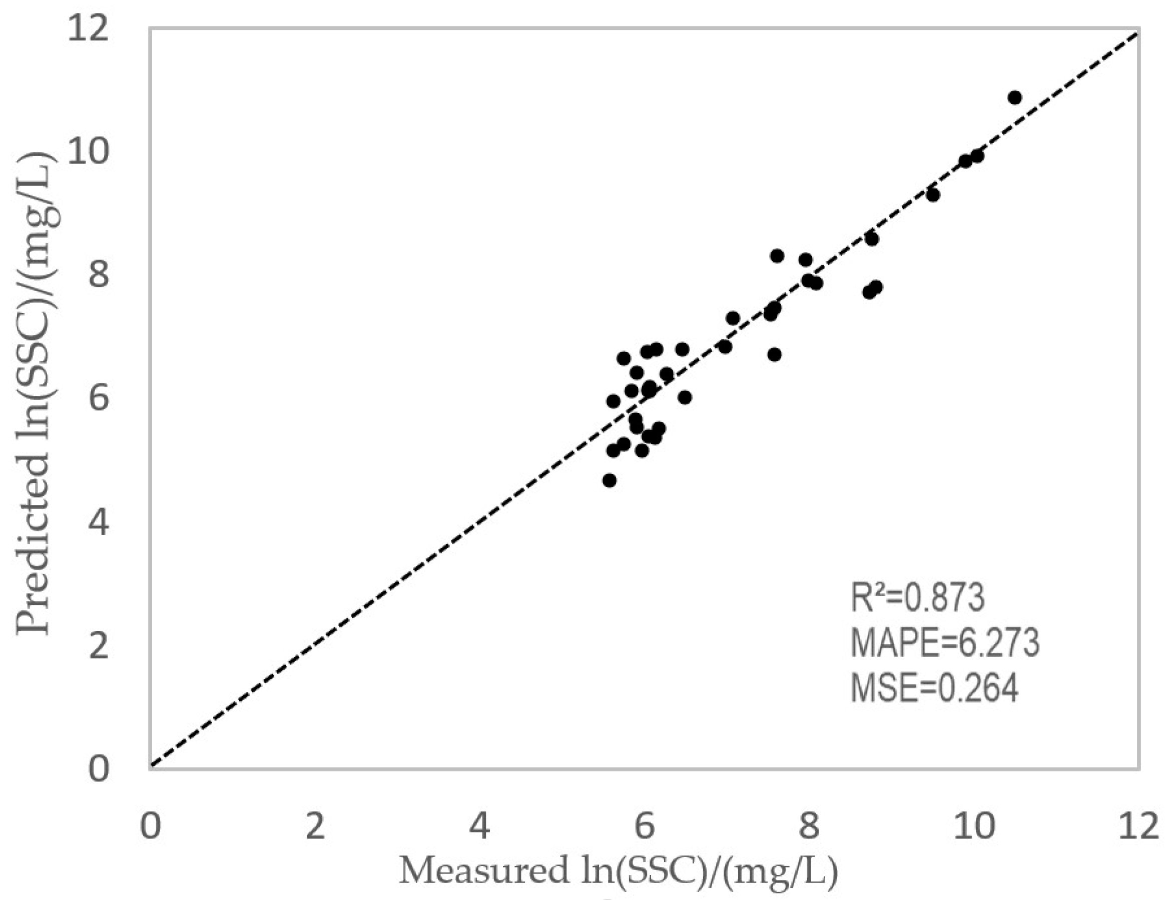
3.1. Suspended Sediment Modeling

In this study, before applying the stochastic forest regression model, we also tried other models, and the best fitting effect of each model is shown in

Table 1. Best fitting performance of each model on the training set.

Model Type	Basis for Classification	Sample Number	Testing ln(SSC) R2	MSE	MAPE
Random Forest	Overall	124	0.873	0.264	6.273
	High-water period	45	0.683	0.442	8.046
	Low-water period	79	0.808	0.325	7.197
	Spring	31	0.717	0.334	7.066
	Summer	32	0.742	0.389	6.19
	Autumn	30	0.754	0.341	7.407
	Winter	31	0.551	0.208	6.094
Linear Regression	Overall	124	0.731	0.488	8.402
	High-water period	45	0.699	0.947	10.924
	Low-water period	79	0.573	0.443	8.327
	Spring	31	0.538	0.456	10.288
	Summer	32	0.742	0.529	9.049
	Autumn	30	0.746	0.431	7.855
	Winter	31	0.534	0.247	7.534
Back Propagation Neural Network	Overall	124	0.842	0.281	6.719
	High-water period	45	0.619	0.467	8.925
	Low-water period	79	0.775	0.292	5.852
	Spring	31	0.695	0.348	7.197
	Summer	32	0.711	0.401	6.952
	Autumn	30	0.679	0.342	6.113
	Winter	31	0.451	0.307	7.185
Support Vector Regression	Overall	124	0.746	0.298	6.941
	High-water period	45	0.548	0.435	8.713
	Low-water period	79	0.620	0.516	7.721
	Spring	31	0.640	0.351	7.244
	Summer	32	0.779	0.356	5.818
	Autumn	30	0.563	0.466	6.692
	Winter	31	0.377	0.391	7.668

.

In each model, there are individual cases with high fitting accuracy in each attribute classification. For example, when using a back propagation neural network (BP neural network) model to fit the overall sample, its R² can reach 0.842. The fitting accuracy of the support vector machine model is relatively unstable, and its R² fluctuates from 0.779 to 0.377. Among all models, the random forest model shows the most stable performance across different scenarios. When applied to seasonal and hydrological classifications, the average R² of the random forest model reaches 0.733, and the average MSE is 0.329, indicating a strong generalization ability. Additionally, when fitting the overall dataset, the random forest model achieves an R² of 0.873, reflecting its excellent fitting capacity on the full sample. Therefore, the random forest model outperforms other models in both accuracy and robustness.

Following [48,49], this study combines the bands by division, subtraction, and the normalized difference index form to fit the ln(SSC). The normalized difference index form is derived from the Normalized Difference Vegetation Index (NDVI). The calculation formula is (B_i − B_j)/(B_i + B_j), where B represents the reflectivity of the band in the remote sensing image, and the subscript i and j represent the band number. Each band is entered into the model for linear fitting using the exhaustive method. The combination bands with a relatively high R² and a low MSE will be selected.

Table 2. Linear fit effect.

Modeling Variables	MSE	MAPE	R2	Formula
X = B8	0.99	11.05	0.453	Y = 0.001269 X + 5.361
X = B8A	1.03	11.43	0.426	Y = 0.001112 X + 5.629
X = B5/B3	0.53	8.26	0.706	Y = 4.937 X + 1.196
X = B6/B1	0.53	8.60	0.704	Y = 1.808 X + 4.242
X = B6/B2	0.50	8.28	0.722	Y = 2.24 X + 4.193
X = B7/B1	0.52	8.39	0.712	Y = 1.672 X + 4.427
X = B7/B2	0.51	8.35	0.717	Y = 2.034 X + 4.422
X = B8/B1	0.53	8.58	0.706	Y = 1.724 X + 4.529
X = B8/B2	0.51	8.31	0.717	Y = 2.118 X + 4.502
X = B8A/B1	0.51	8.51	0.716	Y = 1.617 X + 4.897
X = B8 − B1	0.52	8.65	0.715	Y = 0.002047 X + 6.239
X = B8 − B2	0.50	8.59	0.722	Y = 0.002132 X + 6.53
X = B8 − B3	0.51	8.63	0.718	Y = 0.002345 X + 7.356
X = B11 − B6	0.52	8.26	0.713	Y = −0.002 X + 5.265
X = B11 − B8A	0.49	8.24	0.732	Y = −0.001851 X + 5.677
X = B12 − B6	0.51	8.26	0.721	Y = −0.001979 X + 5.159
X = B12 − B7	0.50	8.29	0.722	Y = −0.001831 X + 5.26
X = B12 − B8	0.49	8.20	0.729	Y = −0.001935 X + 5.351
X = B12 − B8A	0.49	8.40	0.730	Y = −0.001809 X + 5.591
X = (B4 − B3)/(B4 + B3)	0.59	8.44	0.675	Y = 15.95 X + 5.958
X = (B5 − B3)/(B5 + B3)	0.58	8.66	0.681	Y = 11.39 X + 6.198
X = (B6 − B2)/(B6 + B2)	0.59	8.91	0.672	Y = 5.599 X + 6.631
X = (B7 − B2)/(B7 + B2)	0.62	9.10	0.658	Y = 5.087 X + 6.679
X = (B8 − B2)/(B8 + B2)	0.62	9.203	0.655	Y = 4.997 X + 6.871

X represents the band or band combination, B represents the band, and Y represents ln(SSC).

displays the band combination results with a better fitting effect.

Table 2 demonstrates that the fitting effect of a single band is subpar, the R² is relatively low, and the MSE is relatively high. For example, the R² of B8 (NIR) is 0.453, and the one of B8A (Red Edge 4) is 0.426. The band combination in the form of a normalized difference index shows no significant improvement in accuracy, and the maximum R² is only 0.681. In contrast, the combination of subtraction and division has higher fitting accuracy. Table 2 shows that the B11-B8A band combination has the highest R² of 0.732 and the lowest MSE of 0.49. It can be seen that the estimation of suspended sediment involves many variables and is affected by many factors. Therefore, a single band cannot be used, and the estimation of suspended sediment by remote sensing requires the participation of multiple variables.

3.2. Sediment Inversion

After a series of experiments, the other parameters of the following random forest model are selected: the evaluation criterion of node splitting is MSE, the number of decision trees is 500, the sampling is put back, the maximum depth of trees is 20, and the maximum number of leaf nodes is 50.

The sample points are grouped according to seasonal or hydrological conditions. First, linear fitting is carried out for each band. Then, the band combination with the best fitting effect (between 25 and 30) is selected and added to the random forest regression model.

Table 3. Results of random forest regression based on different classifications.

Basis for Classification	Sample Number	Training ln(SSC) R2	Testing ln(SSC) R2
Overall	124	0.956	0.873
High-water period	45	0.965	0.683
Low-water period	79	0.895	0.808
Spring	31	0.957	0.717
Summer	32	0.916	0.742
Autumn	30	0.924	0.754
Winter	31	0.841	0.551

The table shows the model with the highest prediction accuracy of the training set in each group and the accuracy of its application to the testing set. The high-water period is from June to October, and the rest of the time comprises the low-water period. The natural logarithm was taken from all input data.

lists the results of the regression modeling. The random forest method proved to be quite robust, as expected. All SSC tests, excluding conducted in summer, have an R² greater than 0.7 and an average R² of 0.79. This shows that using the random forest model to monitor the suspended sediment concentration is feasible.

The random forest model determines the relative importance of each variable in the model by evaluating and ranking the contribution of each variable to the improvement of the model’s prediction accuracy. The greater the variable’s importance, the higher its contribution to the model’s prediction accuracy.

Figure 2 depicts the overall inversion results of the SSC. It indicates that as the number of variables changes, the prediction accuracy of each sub-model will gradually reach a relatively stable state. When all band combinations are added to the model, the obtained prediction accuracy is not the best. In contrast, the most accurate model prediction will result from choosing several variables. In addition, too many variables will lead to difficulty in interpretation. Therefore, when rebuilding the model, it is unnecessary to add too many variables to achieve maximum accuracy. When all samples participate in modeling, the band combination of (B4 − B3)/(B4 + B3), B8 − B1, B7/B1, B12 − B8A, and B8 − B3 has the best inversion effect, and the R² is 0.873, where the band combination with the greatest feature importance is (B4 − B3)/(B4 + B3).

Figure 3 displays the inversion results of the SSC by water regime classification. In the dry season, the band combination of B11 − B8A, B8/B4, B8 − B4, B8A − B5, B12 − B8A, B7/B3, (B8A − B1)/(B8A + B1), and B8A/B2 has the best inversion effect, and the R² is 0.808. The band combination with the greatest feature importance is B11 − B8A. In the wet season, the band combination of B9 − B8, B4 − B3, B9 − B7, B9 − B6, and B11 − B8 has the best inversion effect; the R² is 0.683, and the band combination with the most important feature is B9 − B8.

Figure 4 shows the inversion results of the SSC by season classification. The inversion effect varies from season to season. The best inversion effect is in autumn, when the band combination is B4/B5, B5 − B4, (B5 − B4)/(B5 + B4), B3/B7, B6 − B3, B5/B4, and B3/B6, and the R² is 0.754. The worst inversion performance is observed in winter, where even the highest R² value only reaches 0.551, which is significantly lower than that of other seasons. The band combination with the most important feature is B5/B3, where the value of feature importance reaches 0.24. In summer, the inversion effect of 6 – 7 band combinations is the best, and the R² is above 0.73. The redundant band combinations will make the inversion effect worse. In spring, the inversion results are good when the second band combination is added.

Producing a comparison by classifying with different attributes, the optimal feature combinations obtained in Figure 2 through Figure 4 are different. The Red band B4 (664 nm) and the Red Edge band B8A (864 nm) appear most frequently in the variable combinations when each model achieves the highest prediction accuracy, indicating that they are the most influential bands in the random forest prediction model.

When all sample points are added to the random forest, the combination of (B4 − B3)/(B4 + B3), B8 − B1, B7/B1, B12 − B8A, and B8 − B3 produces the most effective inversion impact. Figure 5 illustrates a scatter plot of predicted ln(SSC) and actual ln(SSC). It indicates that the R² is 0.873, the MSE is 6.273%, and the MAPE is 0.264 for the ln(SSC) calculated by random forest. It also shows that using the random forest model is feasible to monitor the suspended sediment concentration.

Figure 6 displays the impact of the suspension sediment validation set at the Longmen Station. At this time, the R² is 0.94, and the average absolute percentage error is 38.32%. This indicates that in most cases, this model has relatively accurate results and can predict the suspended sediment concentration. However, there are also instances where the inversion accuracy is poor (points 9, 14, and 27). This shows that the model is still not perfect for prediction, and there is room for further development.

3.3. Sediment Spatial Distribution

Taking the river section around Yumen Kou as the study area, a better inversion image is selected every month in 2020 to invert the annual sediment discharge from the outlet of the Yellow River canyon, as shown in Figure 7.

It can be seen from the figure that the water volume and sediment concentration of the Yellow River have changed greatly in this year. In terms of the width of the river, March, July, August, and September are obviously wider than other months, and January and December are the narrowest, reflecting abundant rainfall in summer and the scarcity of rainwater in winter. However, August and September are also the months with high sediment concentration, and the sediment concentration in January and December is also very low, indicating that there is a positive correlation between water volume and sediment concentration.

Referring to the literature, we can see that one of the main sources of sediment in the Yellow River is scouring by rainwater. Rainwater in the rainy season enters the Yellow River with sediment from the Loess Plateau, which is consistent with the image. Although the river is wide in March, the low sediment concentration is due to the melting of snow and ice in the upper reaches, which increases the flow of the Yellow River and does not bring sediment from the Loess Plateau.

From the perspective of sediment distribution, taking YuMen Kou as the boundary, when the sediment concentration is extremely high, the sediment concentration in the Yellow River canyon exceeds that in the Xiaobei mainstream. Conversely, when the sediment concentration is relatively low, the sediment concentration in the Xiaobei mainstream surpasses that in the Yellow River canyon. This significant difference in sediment distribution between the Yellow River canyon and the Xiaobei mainstream can be attributed to their distinct topographies: the narrow terrain of the Yellow River canyon and the open landscape of the Xiaobei mainstream. When the total sediment concentration is high, sediment accumulates in the Yellow River canyon due to its confined topography, whereas sediment disperses in the Xiaobei mainstream. On the other hand, during periods of low sediment content, a substantial amount of sediment continues to enter the water in the floodplain of the Xiaobei mainstream. Another characteristic of sediment distribution is that the concentration near the riverbanks is higher, while the concentration at the river center is lower, which is particularly evident in April, May, June, and August. Examining the variation in sediment concentration around YuMen Kou in 2020, it was observed that due to abundant rainfall in summer, the sediment concentration peaks at up to 30,000 mg/L. In contrast, during winter, when rainfall is minimal, the sediment concentration decreases to less than 1000 mg/L. Overall, the random forest algorithm effectively represents the sediment concentration in waters near the YuMen Kou site.

4. Discussion

In terms of the spatiotemporal distribution of suspended sediment, there are obvious seasonal variations in the water volume and sediment concentration of the Yellow River. During the high-water-level flood season (July–September), the water volume is large and the sediment content is high, while during the dry season (January and December in winter), the water volume is small and the sediment content is low, which is consistent with the monitoring structure using Landsat remote sensing by Duan, Qiu [2]. Similarly, Qiu, Liu [50] also pointed out, based on 40 years of data analysis, that the sediment content of the Yellow River is the highest in summer and autumn (averaging about 2998 mg/L), and the lowest in winter and spring (about 1126 mg/L). The canyon sections with narrow terrain have a high sediment content, while the meandering sections with open rivers are prone to sediment diffusion and have a relatively lower concentration. The sediment concentration on the cross-section of the river channel shows a distribution pattern of “high near the bank and low in the center”, and this phenomenon is particularly obvious in spring and summer. This is consistent with the results of another study comparing the suspended sediment concentrations at different transverse positions in the cross-section using GF-1 remote sensing [51]. Studies on the Sanmenxia–Xiaolangdi–Yumenkou Canyon of the Yellow River and the downstream wandering section also suggest that in the canyon section (where the river channel is narrow), the concentration of suspended sediment remains at a high level and sediment transport is concentrated. After entering the open “Xiaobei mainstream” downstream, the sediment diffuses on the wider water surface, and the concentration decreases significantly [52].

The results indicate that bands B4, B7, B8A, and B9 are particularly responsive to sediment inversion in high-concentration sediment environments. This finding aligns with previous studies [53]. Since changes in wavelength result in variations in water body reflectivity, the blue-green band absorbs less sunlight, whereas the near-infrared band exhibits strong absorption capabilities. When sediment particles are present in water, the reflection spectrum curve alters due to sediment scattering, leading to an increase in band reflectance. The peaks of band reflectance occur in the yellow and red bands, which correspond well with field-measured water body remote sensing reflectance data reported by others [54], and the monitoring results for the transport of suspended sediment in the lower reaches of the Yellow River also support this view [2]. Furthermore, by combining sensitive and non-sensitive bands through their spectral indices’ ratio, difference, or normalized difference index forms, a good prediction effect can be achieved. This is likely due to their ability to suppress systematic noise (e.g., residual atmospheric effects) and enhance SSC-related spectral signals [55]. Ratios and normalized differences, in particular, can highlight turbidity-induced reflectance changes, thereby increasing sensitivity to sediment variability in high-SSC waters such as the Yellow River [56,57]. Various specific operations arise from different band combinations, indicating that estimating suspended sediment concentrations involves multiple variables and is influenced by various factors. This process is complex, and using certain estimated frequency bands alone is insufficient [58]. A relatively high correlation exists between the predicted values calculated using the random forest model and the measured values. Additionally, both the mean squared error (MSE) and the mean absolute percentage error (MAPE) are satisfactory, suggesting that the random forest model is feasible for monitoring suspended sediment concentration.

However, the data accuracy in summer remains very low. Due to the abundant rainfall in August and September, a large amount of sediment from the upper reaches flows into the Yellow River, resulting in an increase in sediment content and the river channel area reaching the largest of the year [59]. The weather warmed up in March, and the snow and ice in the mountains near the source of the Yellow River melted a lot, and the amount of water and sediment in the middle and lower reaches increased. Taking YuMen Kou as the boundary, the reason for the significant difference in sediment distribution between the upstream and downstream is that the upstream terrain is narrow, and the downstream is open. When the sediment concentration is high in summer, the upstream sediment is deposited, and the downstream is dispersed. On the other hand, when the overall sediment concentration is low in the other seasons, the turbulent upstream water brings the sediment downstream, and the floodplain in the downstream river still has a large sediment amount brought into the water.

Furthermore, although this study has achieved good results in inverting the concentration of highly suspended sediments in the Yellow River by using Sentinel-2 remote sensing data and the random forest model, there are still certain limitations that need to be addressed in subsequent studies.

• Spatiotemporal offsets of remote sensing pixels and hydrological stations: The remote sensing images used in this study provide the instantaneous reflection information of the water surface layer, reflecting the reflectivity of suspended solids on the water surface. However, the hydrological stations measure the average sediment content within a certain depth range of the cross-section, and there are differences in the data nature between the two [60]. To reduce the influence of mixed pixels along the bank and human interference, this paper selects the pixels in the central area of the river channel for matching to improve the inversion stability. However, even if they are located at the same section, the spatial offset between the remote sensing pixels and the measured points may still cause errors. The matching strategy should be optimized in the future. Although existing studies have shown that under high-SSC conditions, suspended particles in water bodies are uniformly distributed, the SSC estimation based on surface reflectance data by remote sensing inversion is statistically representative [61,62]. However, on-site spectral verification can evaluate the reliability of remote sensing models and further enhance the calibration and physical interpretation of inversion models.
• The sample size is limited: This research model is established based on the data from 2019 to 2020. With a limited time span, it may be difficult to comprehensively reflect the interannual and seasonal variations in the Yellow River Basin. The study area is located in a mountainous region with cloudy and foggy weather. Some images were eliminated due to weather conditions, and ultimately only 128 valid images were obtained, approximately 30 per season. Limited samples pose challenges to the training of machine learning models, especially in seasonal inversion. Although this site provides high-quality SSC data, as a single upstream site, it is difficult to represent the hydrological characteristics of the entire basin, especially in the downstream areas where the terrain, tributary input, and human activities are significantly different.
• Other factors: The river section where Longmen Station is located is mountainous. Runoff and topography are the dominant factors affecting the distribution of suspended sediment, and meteorological and hydrological conditions also play a significant role [63,64]. In the variable selection of this paper, only paired band combinations were used. However, Sentinel-2 has higher-dimensional band information. Although the combination of three or four bands may improve the model performance, it also increases the complexity of interpretation. Its potential can be further explored in the future.

Therefore, future research should verify the adaptability of the model within a broader temporal and spatial range, especially by introducing multisite monitoring data in the lower reaches of the Yellow River region to enhance the spatial generalization ability of the model. Meanwhile, the biological optical model can be combined to explore the optical characteristic mechanism of suspended particles in high-turbidity water bodies, and the remote sensing inversion results can be verified through ground spectral and radiation observations to solve the possible reflectance saturation problem under high-SSC conditions. In addition, in the future, more band combinations and environmental variables can be introduced to construct a composite model with greater physical significance and application value.

5. Conclusions

For thousands of years, the Yellow River has been plagued by sediment-related issues. Although increasing attention has been paid to the ecological problems of the Yellow River in recent years, and certain improvements have been achieved, sediment remains a critical concern. Satellite remote sensing provides a promising approach for understanding the spatiotemporal dynamics of suspended sediments at a macroscale. In this study, high Suspended Sediment Concentrations (SSC) in the Yellow River Basin were estimated using Sentinel-2 imagery and a random forest model. This not only expands the applicability of multispectral remote sensing in complex river systems but also demonstrates the strengths of the random forest algorithm in handling nonlinear relationships and high-dimensional variable combinations. Compared with traditional linear regression models, the random forest model offers higher accuracy and greater flexibility when applied to complex aquatic environments, particularly in high-turbidity water bodies. The feature importance ranking further enables the identification of key spectral bands influencing the SSC, providing valuable support for subsequent variable interpretation.

Moreover, the proposed method proves to be effective for remote sensing-based SSC monitoring in the Yellow River. Among Sentinel-2 MSI bands, the red band (B4) and near-infrared band (B8A) were identified as significant predictors of the SSC in the random forest model. Additionally, the integration of both sensitive and non-sensitive bands improved inversion accuracy. The random forest models for the dry and wet seasons achieved an average fitting accuracy of 0.735 and an average relative RMSE of 6.08%, demonstrating the model’s high precision in estimating suspended sediment concentration (SSC). Based on 2020 data, this study found that the SSC varies significantly with the seasons. In summer, with abundant rainfall, the SSC can reach 30,000 mg/L, while in winter, it drops to below 1000 mg/L. The spatial distribution of sediment also shows topographical differences: the SSC is higher in the Yellow River Canyon during high total sediment concentrations, while it is lower in the Xiaobei mainstream. Additionally, the SSC is positively correlated with water flow, with higher concentrations observed during the wet season (July–September). These findings suggest that SSC estimation involves multiple interacting variables and is influenced by various environmental factors. Therefore, it is not feasible to rely on a single band for accurate inversion, and a multivariable approach is essential for remote sensing-based SSC estimation.

References

1. Dethier, E.N.; Renshaw, C.E.; Magilligan, F.J. Rapid changes to global river suspended sediment flux by humans. Science 2022, 376, 1447–1452. [Google Scholar] [CrossRef]
2. Duan, M.; Qiu, Z.; Li, R.; Li, K.; Yu, S.; Liu, D. Monitoring Suspended Sediment Transport in the Lower Yellow River using Landsat Observations. Remote Sens. 2024, 16, 229. [Google Scholar] [CrossRef]
3. Wang, Y. Analysis of Influence of Sediment Content on Monitoring Results of River Water Quality. Shanxi Water Resour. 2020, 12, 114–116. (In Chinese) [Google Scholar]
4. UNESCO-ISI. Online Training Workshop on Sediment Transport Measurement and Monitoring. Available online: http://www.waser.cn/waser/NAA/webinfo/2021/07/1627854511860865.htm (accessed on 11 July 2024).
5. Zhang, X.; Fichot, C.G.; Baracco, C.; Guo, R.; Neugebauer, S.; Bengtsson, Z.; Ganju, N.; Fagherazzi, S. Determining the drivers of suspended sediment dynamics in tidal marsh-influenced estuaries using high-resolution ocean color remote sensing. Remote Sens. Environ. 2020, 240, 111682. [Google Scholar] [CrossRef]
6. Aires, U.R.V.; da Silva, D.D.; Fernandes Filho, E.I.; Rodrigues, L.N.; Uliana, E.M.; Amorim, R.S.S.; de Melo Ribeiro, C.B.; Campos, J.A. Modeling of surface sediment concentration in the Doce River basin using satellite remote sensing. J. Environ. Manag. 2022, 323, 116207. [Google Scholar] [CrossRef]
7. Zhang, S.; Zhao, Z.; Li, G.; Wu, J.; Wang, Y.G.; Nielsen, P.; Jeng, D.S.; Qiao, L.; Wang, C.; Li, S. Estimation of sediment transport parameters from measured suspended concentration time series under waves and currents with a new conceptual model. Water Resour. Res. 2024, 60, e2023WR034933. [Google Scholar] [CrossRef]
8. Cai, L.; Zhou, M.; Liu, J.; Tang, D.; Zuo, J. HY-1C observations of the impacts of islands on suspended sediment distribution in Zhoushan coastal waters, China. Remote Sens. 2020, 12, 1766. [Google Scholar] [CrossRef]
9. Zhang, M.; Guo, B. Retrieval of Suspended Sediment Concentration in Zhoushan Coastal Area Satellite Based on GF-1. Ocean. Dev. Manag. 2018, 35, 126–131. (In Chinese) [Google Scholar]
10. Fan, J.; Liu, X.; Li, W. Daily suspended sediment concentration forecast in the upper reach of Yellow River using a comprehensive integrated deep learning model. J. Hydrol. 2023, 623, 129732. [Google Scholar] [CrossRef]
11. Xie, J.; Feng, X.; Gao, T.; Wang, Z.; Wan, K.; Yin, B. Application of deep learning in predicting suspended sediment concentration: A case study in Jiaozhou Bay, China. Mar. Pollut. Bull. 2024, 201, 116255. [Google Scholar] [CrossRef]
12. Yan, J.; Xu, Z.; Yu, Y.; Xu, H.; Gao, K. Application of a hybrid optimized BP network model to estimate water quality parameters of Beihai Lake in Beijing. Appl. Sci. 2019, 9, 1863. [Google Scholar] [CrossRef]
13. Peterson, K.T.; Sagan, V.; Sidike, P.; Cox, A.L.; Martinez, M. Suspended Sediment Concentration Estimation from Landsat Imagery along the Lower Missouri and Middle Mississippi Rivers Using an Extreme Learning Machine. Remote Sens. 2018, 10, 1503. [Google Scholar] [CrossRef]
14. Stull, T.; Ahmari, H. Estimation of suspended sediment concentration along the lower brazos river using satellite imagery and machine learning. Remote Sens. 2024, 16, 1727. [Google Scholar] [CrossRef]
15. Aires, U.R.V.; da Silva, D.D.; Fernandes Filho, E.I.; Rodrigues, L.N.; Uliana, E.M.; Amorim, R.S.S.; de Melo Ribeiro, C.B.; Campos, J.A. Machine learning-based modeling of surface sediment concentration in Doce river basin. J. Hydrol. 2023, 619, 129320. [Google Scholar] [CrossRef]
16. Sagan, V.; Peterson, K.T.; Maimaitijiang, M.; Sidike, P.; Sloan, J.; Greeling, B.A.; Maalouf, S.; Adams, C. Monitoring inland water quality using remote sensing: Potential and limitations of spectral indices, bio-optical simulations, machine learning, and cloud computing. Earth-Sci. Rev. 2020, 205, 103187. [Google Scholar] [CrossRef]
17. Breiman, L. Random forests. Mach. Learn. 2001, 45, 5–32. [Google Scholar] [CrossRef]
18. Fang, X.; Wen, Z.; Chen, J.; Wu, S.; Huang, Y.; Ma, M. Remote sensing estimation of suspended sediment concentration based on Random Forest Regression Model. J. Remote Sens. 2019, 23, 756–772. (In Chinese) [Google Scholar] [CrossRef]
19. Dehkordi, A.T.; Ghasemi, H.; Zoej, M.J.V. Machine Learning-Based Estimation of Suspended Sediment Concentration along Missouri River using Remote Sensing Imageries in Google Earth Engine. In Proceedings of the 2021 7th International Conference on Signal Processing and Intelligent Systems (ICSPIS), Tehran, Iran, 29–30 December 2021; pp. 1–5. [Google Scholar]
20. Gu, K.; Zhang, Y.H.; Qiao, J.F. Random Forest Ensemble for River Turbidity Measurement From Space Remote Sensing Data. Ieee Trans. Instrum. Meas. 2020, 69, 9028–9036. [Google Scholar] [CrossRef]
21. Park, E.; Latrubesse, E.M. Surface water types and sediment distribution patterns at the confluence of mega rivers: The Solimoes-Amazon and Negro Rivers junction. Water Resour. Res. 2015, 51, 6197–6213. [Google Scholar] [CrossRef]
22. Oxford, M. Remote sensing of suspended sediments in surface waters. Photogramm. Eng. Remote Sens 1976, 42, 1539–1545. [Google Scholar]
23. Umar, M.; Rhoads, B.L.; Greenberg, J.A. Use of multispectral satellite remote sensing to assess mixing of suspended sediment downstream of large river confluences. J. Hydrol. 2018, 556, 325–338. [Google Scholar] [CrossRef]
24. Mangiarotti, S.; Martinez, J.M.; Bonnet, M.P.; Buarque, D.C.; Filizola, N.; Mazzega, P. Discharge and suspended sediment flux estimated along the mainstream of the Amazon and the Madeira Rivers (from in situ and MODIS Satellite Data). Int. J. Appl. Earth Obs. Geoinf. 2013, 21, 341–355. [Google Scholar] [CrossRef]
25. Larson, M.D.; Simic Milas, A.; Vincent, R.K.; Evans, J.E. Landsat 8 monitoring of multi-depth suspended sediment concentrations in Lake Erie’s Maumee River using machine learning. Int. J. Remote Sens. 2021, 42, 4064–4086. [Google Scholar] [CrossRef]
26. YRCC. Yellow River Sediment Bulletin. Available online: http://www.yrcc.gov.cn/gzfw/nsgb/ (accessed on 18 November 2022).
27. Ning, Z.; Gao, G.; Fu, B. Characteristics and Attribution Analysis of Sediment Yield Changes in Helong Region of the Yellow River. Res. Soil Water Conserv. 2022, 29, 38–42. (In Chinese) [Google Scholar]
28. Zhang, P.; Cai, Q.; Zheng, M.; He, T. Spatial and Temporal Distribution of Precipitation in Hekou-Longmen Region and lts Relationship with Sediment Yield. Bull. Soil Water Conserv. 2020, 40, 25–31. (In Chinese) [Google Scholar]
29. Li, C.; Yu, Q.; Gong, X.; Yang, L.; Cao, Y. Remote Sensing Monitoring of Sediment Content Variation in Lower Reach of Yellow River since 1980s. Environ. Sci. Manag. 2020, 45, 165–170. [Google Scholar]
30. Li, J.; Hao, Y.L.; Zhang, Z.Z.; Li, Z.P.; Yu, R.H.; Sun, Y. Analyzing the distribution and variation of Suspended Particulate Matter (SPM) in the Yellow River Estuary (YRE) using Landsat 8 OLI. Reg. Stud. Mar. Sci. 2021, 48. [Google Scholar] [CrossRef]
31. Qiu, Z.F.; Xiao, C.; Perrie, W.; Sun, D.Y.; Wang, S.Q.; Shen, H.; Yang, D.Z.; He, Y.J. Using Landsat 8 data to estimate suspended particulate matter in the Yellow River estuary. J. Geophys. Res.-Ocean. 2017, 122, 276–290. [Google Scholar] [CrossRef]
32. Wang, S.; Shen, M.; Ma, Y.; Chen, G.; You, Y.; Liu, W. Application of Remote Sensing to Identify and Monitor Seasonal and Interannual Changes of Water Turbidity in Yellow River Estuary, China. J. Geophys. Res. Oceans 2019, 124, 4904–4917. [Google Scholar] [CrossRef]
33. Batista, L.V. Turbidity classification of the Paraopeba River using machine learning and Sentinel-2 images. IEEE Lat. Am. Trans. 2022, 20, 799–805. [Google Scholar] [CrossRef]
34. Tian, Z.; Li, Z.; Zhu, J.; Xue, Z.; Zhao, Y. Seasonal Variation of Suspended Sediments in the Yongding New River Estuary from 2017 to 2021. In Proceedings of the IEEE International Geoscience and Remote Sensing Symposium (IGARSS 2022), Kuala Lumpur, Malaysia, 17–22 July 2022. [Google Scholar]
35. Tripathi, G.; Pandey, A.C.; Parida, B.R. Spatio- Temporal Analysis of Turbidity in Ganga River in Patna, Bihar Using Sentinel-2 Satellite Data Linked with COVID-19 Pandemic. In Proceedings of the 2020 IEEE India Geoscience and Remote Sensing Symposium (InGARSS), Ahmedabad, India, 1–4 December 2020; pp. 29–32. [Google Scholar]
36. Fu, J.; Zhang, P.; Zheng, F.; Yinghui, K.; Gao, Y. Dynamic Change Analysis of RainfallErosivity and River Sediment Discharge of He-Long Reach of the Yellow River from 1957 to 2011. Trans. Chin. Soc. Agric. Mach. 2016, 47, 185–192+207. (In Chinese) [Google Scholar]
37. Ouyang, C.; Wang, W.; Tian, Y.; Tian, S. Evaluation on the variation of water-sediment and human activities in the He-Long Reach of the Yellow River over the past 60 years. J. Sediment. Res. 2016, 55–61. [Google Scholar]
38. Li, X.; Jin, S.; Xu, J. Conservation Projects Impacts on Flood and Sediment in Hekouzhen to Longmen Region. Yellow River 2012, 34, 87–89. (In Chinese) [Google Scholar]
39. Li, J.; Xia, J.; Zhu, C. Characteristics and Influencing Factors of Thalweg Migration in the Xiaobeiganliu Reach of the Yellow River During the Period of Continuous Channel Aggradation. J. Basic Sci. Eng. 2022, 30, 883–892. (In Chinese) [Google Scholar]
40. Lin, X.; Dong, C.; Surin, M.; Hu, T. Analysis of the Relationship Between Scouring and Silting and Response of Water and Sediment in Xiaobeiganliu Reach of the Yellow River. Yellow River 2019, 41, 5–8. (In Chinese) [Google Scholar]
41. Xu, J. A Study of Sediment Sink between Longmen and Sanmenxia on the Yellow River. Acta Geogr. Sin. 2009, 64, 515–530. [Google Scholar]
42. Raiyani, K.; Gonçalves, T.; Rato, L.; Salgueiro, P.; Marques da Silva, J.R. Sentinel-2 image scene classification: A comparison between Sen2Cor and a machine learning approach. Remote Sens. 2021, 13, 300. [Google Scholar] [CrossRef]
43. Pahlevan, N.; Sarkar, S.; Franz, B.A.; Balasubramanian, S.V.; He, J. Sentinel-2 MultiSpectral Instrument (MSI) data processing for aquatic science applications: Demonstrations and validations. Remote Sens. Environ. 2017, 201, 47–56. [Google Scholar] [CrossRef]
44. GB T50159–2015; Code for Measurement of Suspended Load in Open Channels. China National Standards: Beijing, China, 2015.
45. Smith, C.; Croke, B.F.W. Sources of uncertainty in estimating suspended sediment load. IAHS-AISH Publ. 2005, 136–143. [Google Scholar]
46. Ismail, R.; Mutanga, O.; Kumar, L. Modeling the Potential Distribution of Pine Forests Susceptible to Sirex Noctilio Infestations in Mpumalanga, South Africa. Trans. GIS 2010, 14, 709–726. [Google Scholar] [CrossRef]
47. Bian, M.; Skidmore, A.K.; Schlerf, M.; Wang, T.J.; Liu, Y.F.; Zeng, R.; Fei, T. Predicting foliar biochemistry of tea (Camellia sinensis) using reflectance spectra measured at powder, leaf and canopy levels. Isprs J Photogramm 2013, 78, 148–156. [Google Scholar] [CrossRef]
48. Wen, Z. Spatial and Seasonal Patterns of Aboveground Net PrimaryProductivity and Their Responses to Environmental Factors in theDrawdown Zone of the Three Gorges Reservoir, China: A Case Studyof Baijiaxi Drawdown Zone. Ph.D. Thesis, Chinese Academy of Sciences, Beijing, China, 2017. [Google Scholar]
49. Yang, J.; Fan, J.; Zhang, Q.; Yu, J.; Zhu, X. Review of suspended sediment content recognition in case II waters by remote sensing. Yangtze River 2019, 50, 98–103. (In Chinese) [Google Scholar]
50. Qiu, Z.; Liu, D.; Duan, M.; Chen, P.; Yang, C.; Li, K.; Duan, H. Four-decades of sediment transport variations in the Yellow River on the Loess Plateau using Landsat imagery. Remote Sens. Environ. 2024, 306, 114147. [Google Scholar] [CrossRef]
51. Yao, R.; Cai, L.; Liu, J.; Zhou, M. GF-1 satellite observations of suspended sediment injection of Yellow River Estuary, China. Remote Sens. 2020, 12, 3126. [Google Scholar] [CrossRef]
52. Xia, X.; Dong, J.; Wang, M.; Xie, H.; Xia, N.; Li, H.; Zhang, X.; Mou, X.; Wen, J.; Bao, Y. Effect of water-sediment regulation of the Xiaolangdi reservoir on the concentrations, characteristics, and fluxes of suspended sediment and organic carbon in the Yellow River. Sci. Total Environ. 2016, 571, 487–497. [Google Scholar] [CrossRef]
53. Sankaran, R.; Al-Khayat, J.A.; Chatting, M.E.; Sadooni, F.N.; Al-Kuwari, H.A.-S. Retrieval of suspended sediment concentration (SSC) in the Arabian Gulf water of arid region by Sentinel-2 data. Sci. Total Environ. 2023, 904, 166875. [Google Scholar] [CrossRef]
54. Lin, L.; Wu, H. Study on Suspended Sediment Concentration Model in Case II Water for the Yellow River Estuary Based on the Spectral Reflectance. Jiangsu Sci. Technol. Inf. 2016, 52–55. (In Chinese) [Google Scholar]
55. Mo, J.; Tian, Y.; Wang, J.; Zhang, Q.; Zhang, Y.; Tao, J.; Lin, J. Remote sensing inversion of suspended particulate matter in the estuary of the Pinglu Canal in China based on machine learning algorithms. Front. Mar. Sci. 2024, 11, 1473104. [Google Scholar] [CrossRef]
56. Pham, Q.V.; Ha, N.T.T.; Pahlevan, N.; Oanh, L.T.; Nguyen, T.B.; Nguyen, N.T. Using Landsat-8 images for quantifying suspended sediment concentration in Red River (Northern Vietnam). Remote Sens. 2018, 10, 1841. [Google Scholar] [CrossRef]
57. Qu, L.; Lei, T.; Ning, D.; Civco, D.; Yang, X. A spectral mixing algorithm for quantifying suspended sediment concentration in the Yellow River: A simulation based on a controlled laboratory experiment. Int. J. Remote Sens. 2016, 37, 2560–2584. [Google Scholar] [CrossRef]
58. Peterson, K.T.; Sagan, V.; Sidike, P.; Hasenmueller, E.A.; Sloan, J.J.; Knouft, J.H. Machine Learning-Based Ensemble Prediction of Water-quality Variables Using Feature-level and Decision-level Fusion with Proximal Remote Sensing. Photogramm. Eng. Remote Sens. 2019, 85, 269–280. [Google Scholar] [CrossRef]
59. Feng, J.; Zhao, G.; Mu, X.; Tian, P. Characteristics and mechanism of sediment transport in the Middle Yellow River. J. Sediment Res. 2020, 45, 34–41. (In Chinese) [Google Scholar]
60. Zhang, H.; Ren, X.; Wang, S.; Li, X.; Sun, D.; Wang, L. Estimating Vertical Distribution of Total Suspended Matter in Coastal Waters Using Remote-Sensing Approaches. Remote Sens. 2024, 16, 3736. [Google Scholar] [CrossRef]
61. Zhang, C.; Liu, Y.; Chen, X.; Gao, Y. Estimation of suspended sediment concentration in the yangtze main stream based on sentinel-2 MSI data. Remote Sens. 2022, 14, 4446. [Google Scholar] [CrossRef]
62. Xiao, X.; Liu, Z.; Liu, K.; Wang, J. Temporal Variation of Suspended Sediment and Solute Fluxes in a Permafrost-Underlain Headwater Catchment on the Tibetan Plateau. Water 2022, 14, 2782. [Google Scholar] [CrossRef]
63. Sun, X.; Zhang, Y.; Shi, K.; Zhang, Y.; Li, N.; Wang, W.; Huang, X.; Qin, B. Monitoring water quality using proximal remote sensing technology. Sci. Total Environ. 2022, 803, 149805. [Google Scholar] [CrossRef]
64. Barnes, B.B.; Hu, C.; Bailey, S.W.; Pahlevan, N.; Franz, B.A. Cross-calibration of MODIS and VIIRS long near infrared bands for ocean color science and applications. Remote Sens. Environ. 2021, 260, 112439. [Google Scholar] [CrossRef]
Figure 1. The geographical locations of the Yellow River Canyon and the sampling reach.
Remotesensing 17 02424 g001
Figure 2. Random forest model SSC inversion result (overall modeling sample number, n = 124). The bar graph represents the importance order of each predictor variable in the random forest regression model, and the line graph represents the fitting accuracy of the model after performing backward variable selection.
Remotesensing 17 02424 g002
Figure 3. Random forest model SSC inversion results (hydrological situation, n = 79,45): (a) in the dry season; (b) in the wet season.
Remotesensing 17 02424 g003
Figure 4. Random forest model SSC inversion results (season, n = 31, 32, 30, 31): (a) spring; (b) summer; (c) autumn; (d) winter.
Remotesensing 17 02424 g004
Figure 5. Overall estimation of suspended sediment in Longmen Station. The dotted line in the figure is the 1:1 line.
Remotesensing 17 02424 g005
Figure 6. Effect of suspended sediment validation set at Longmen Station.
Remotesensing 17 02424 g006
Figure 7. Estimated map of YuMen Kou sediment distribution in 2020.
Remotesensing 17 02424 g007