
TMTS: A Physics-Based Turbulence Mitigation Network Guided by Turbulence Signatures for Satellite Video


Abstract

1. Introduction
2. Materials and Methods
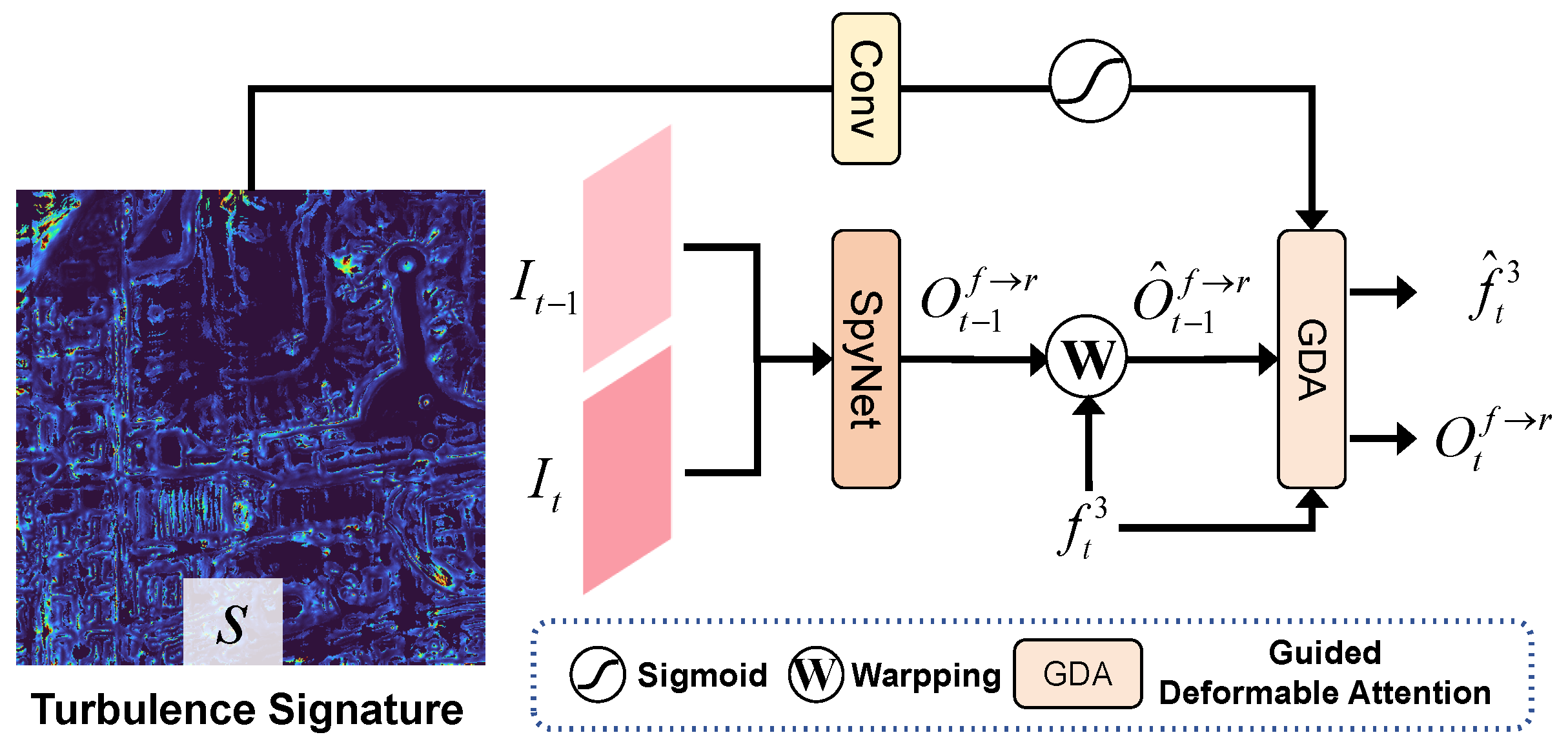
2.1. Turbulence Signature
2.2. TMTS Network
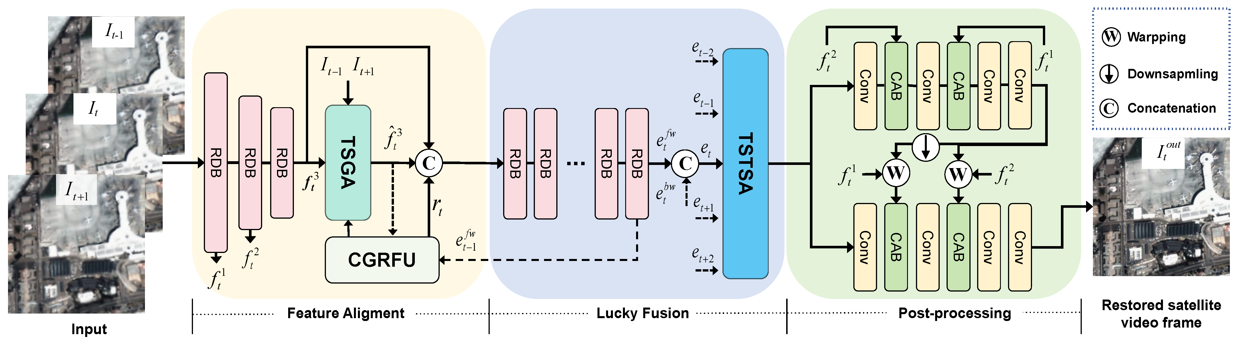
2.2.1. Overview
2.2.2. TSGA Module for Feature Alignment
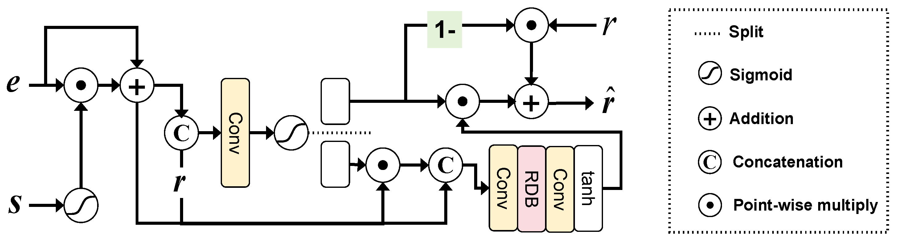
2.2.3. CGRFU Module for Reference Feature Update
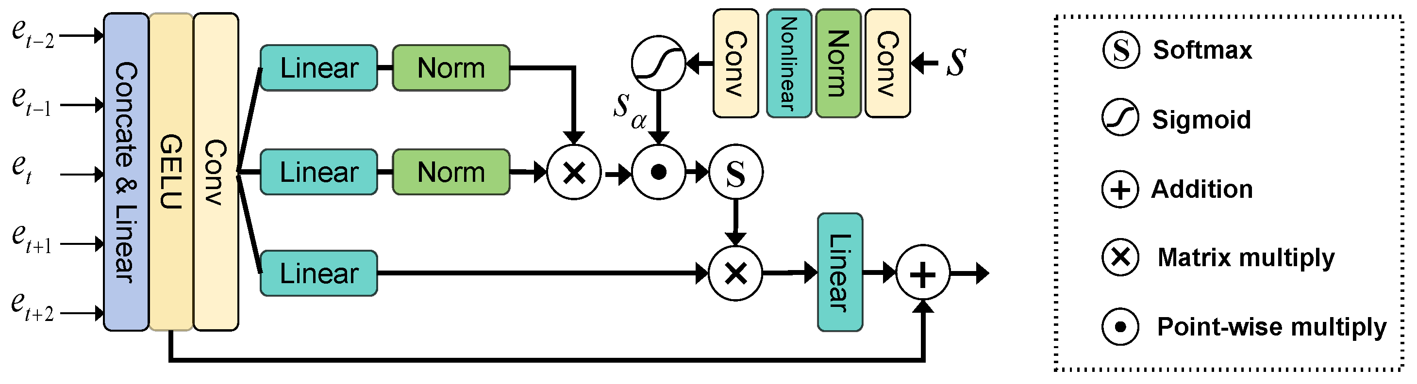
2.2.4. TSTSA for Lucky Fusion
2.2.5. Loss Function
2.3. The Implementation of TMTS
2.3.1. Satellite Video Data Source
2.3.2. Paired Turbulence Data Synthesis
2.3.3. Metrics
2.3.4. Implementation Details
3. Results and Discussion
3.1. Performance on Synthetic Datasets
3.1.1. Quantitative Evaluation
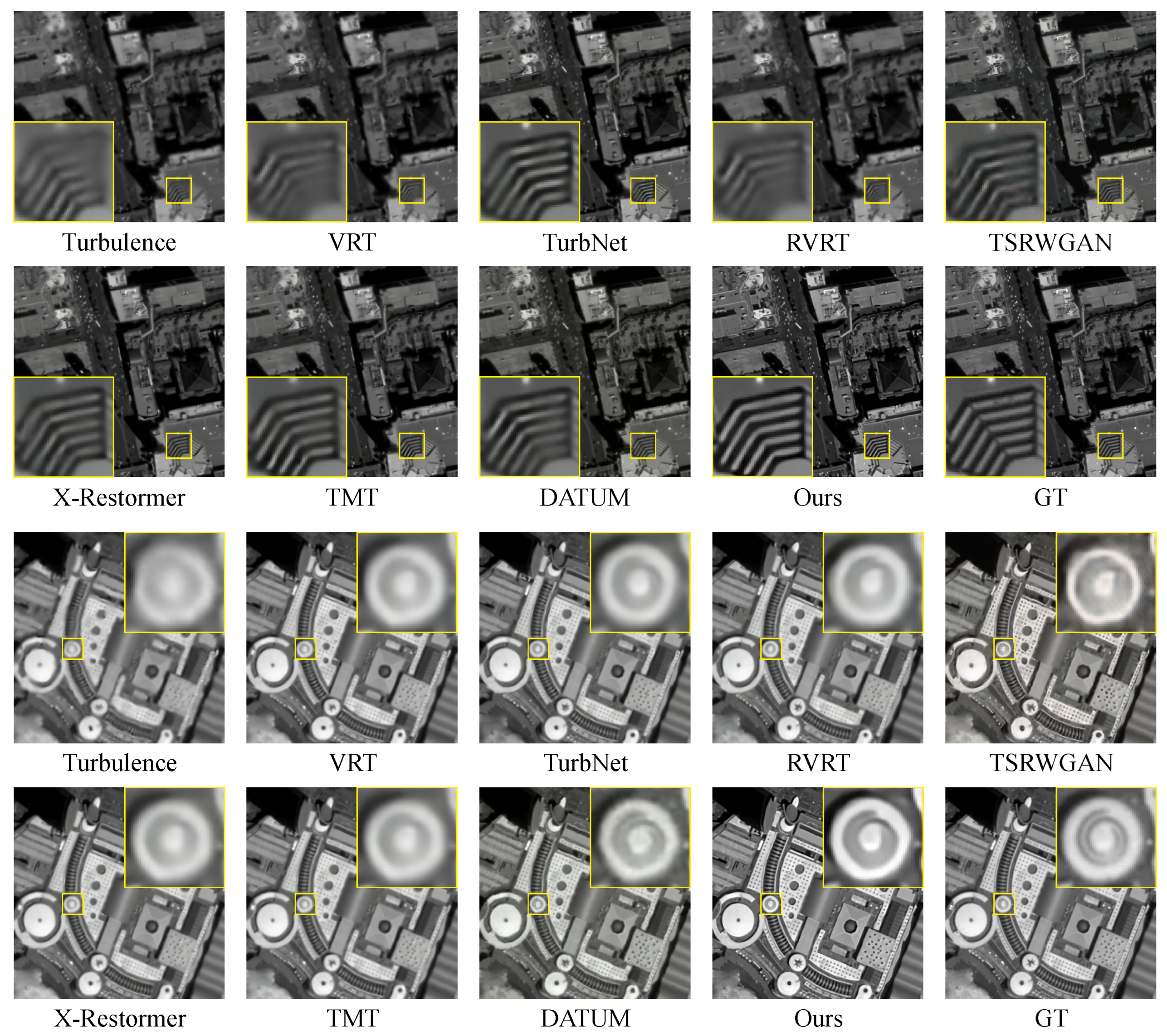
3.1.2. Qualitative Results
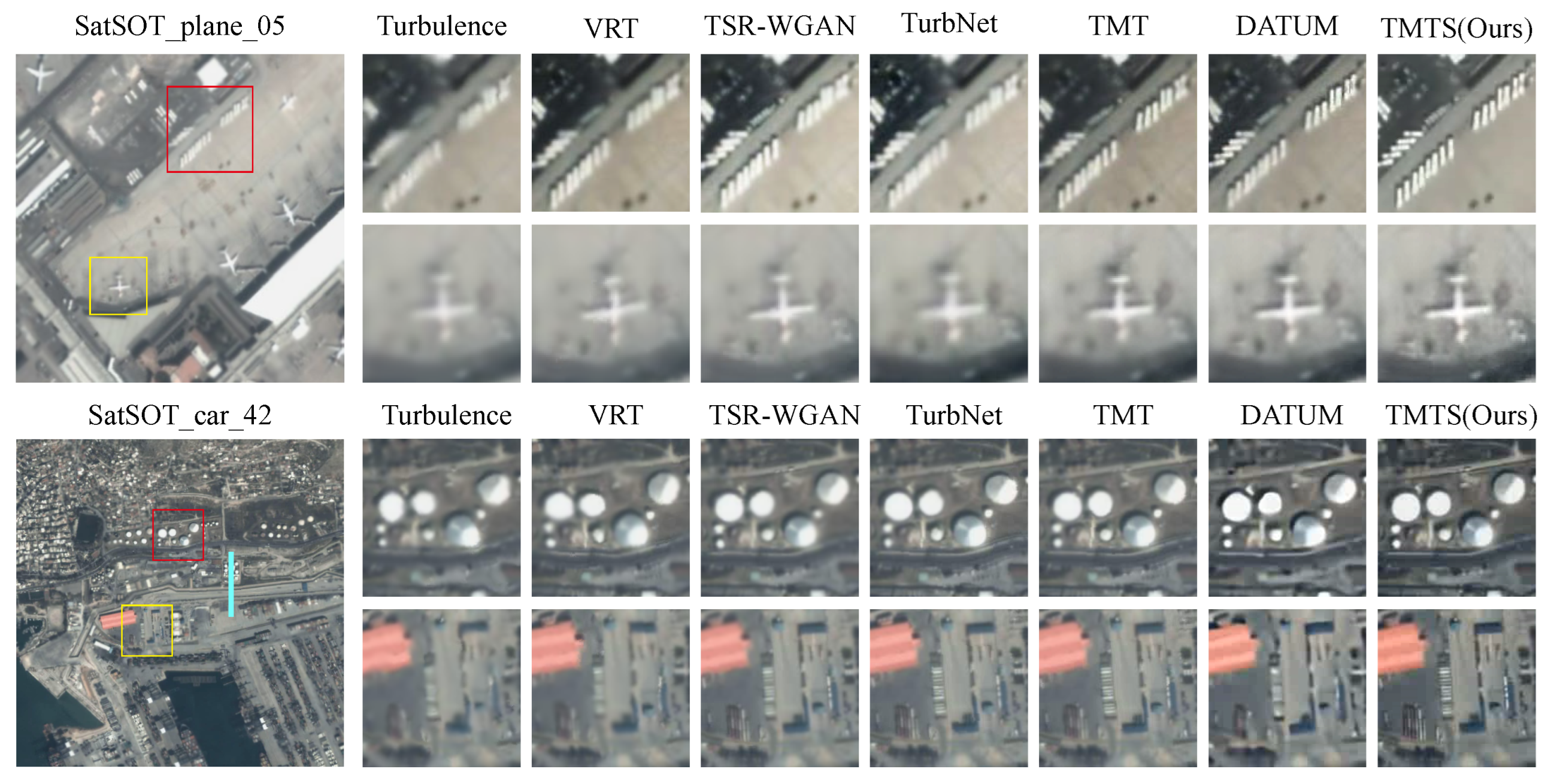
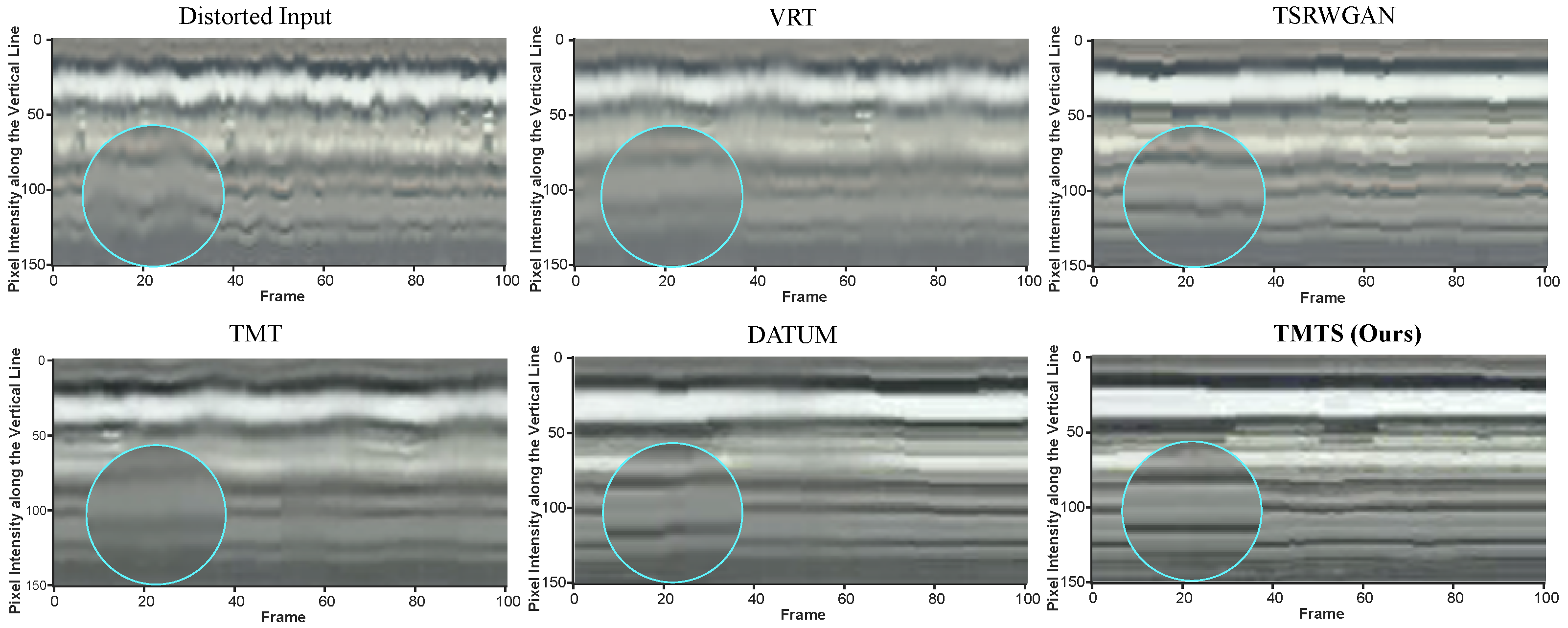
3.2. Performance on Real Data
3.3. Ablation Studies
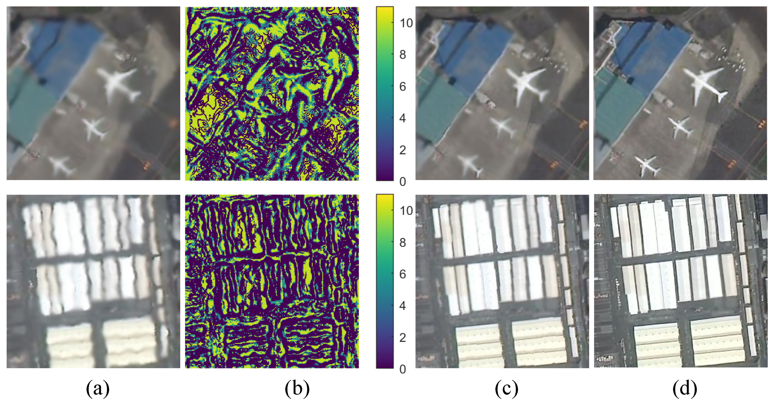
3.3.1. Effect of Turbulence Signature
3.3.2. Effect of TSGA, CGRFU, and TSTSA
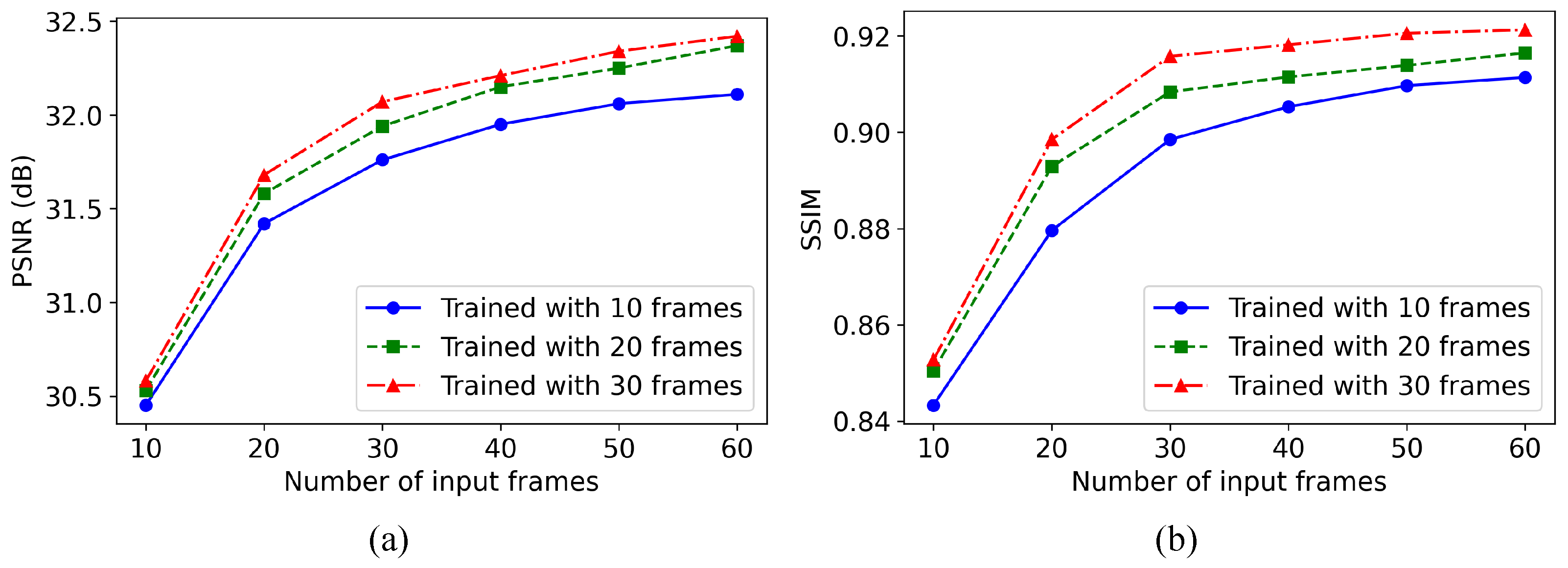
3.3.3. Influence of Input Frame Number
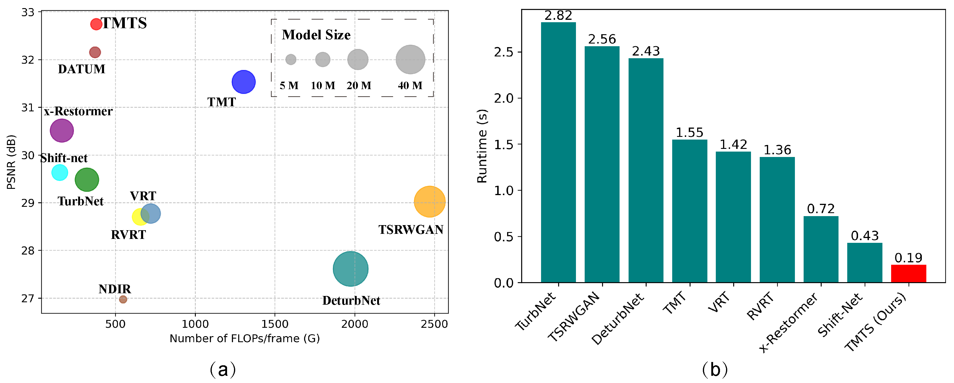
3.3.4. Model Efficiency and Computation Budget
3.4. Limitations and Future Works
- (1)
- Constructing Ground-Truth Turbulence Datasets
- (2)
- Exploring TS Potential
4. Conclusions
Author Contributions
Funding
Data Availability Statement
Conflicts of Interest
References
- Xiao, Y.; Yuan, Q.; Jiang, K.; Jin, X.; He, J.; Zhang, L.; Lin, C.W. Local-Global Temporal Difference Learning for Satellite Video Super-Resolution. IEEE Trans. Circuits Syst. Video Technol. 2024, 34, 2789–2802. [Google Scholar] [CrossRef]
- Zhao, B.; Han, P.; Li, X. Vehicle Perception From Satellite. IEEE Trans. Pattern Anal. Mach. Intell. 2024, 46, 2545–2554. [Google Scholar] [CrossRef] [PubMed]
- Han, W.; Chen, J.; Wang, L.; Feng, R.; Li, F.; Wu, L.; Tian, T.; Yan, J. Methods for Small, Weak Object Detection in Optical High-Resolution Remote Sensing Images: A survey of advances and challenges. IEEE Geosci. Remote Sens. Mag. 2021, 9, 8–34. [Google Scholar] [CrossRef]
- Zhang, Z.; Wang, C.; Song, J.; Xu, Y. Object Tracking Based on Satellite Videos: A Literature Review. Remote Sens. 2022, 14, 3674. [Google Scholar] [CrossRef]
- Rigaut, F.; Neichel, B. Multiconjugate Adaptive Optics for Astronomy. Annu. Rev. Astron. Astrophys. 2018, 56, 277–314. [Google Scholar] [CrossRef]
- Liang, J.; Williams, D.; Miller, D. Supernormal vision and high-resolution retinal imaging through adaptive optics. J. Opt. Soc. Am. A 1997, 14, 2884–2892. [Google Scholar] [CrossRef]
- Law, N.; Mackay, C.; Baldwin, J. Lucky imaging: High angular resolution imaging in the visible from the ground. Astron. Astrophys. 2006, 446, 739–745. [Google Scholar] [CrossRef]
- Joshi, N.; Cohen, M. Seeing Mt. Rainier: Lucky Imaging for Multi-Image Denoising, Sharpening, and Haze Removal. In Proceedings of the 2010 IEEE International Conference on Computational Photography (ICCP 2010), Cambridge, MA, USA, 29–30 March 2010; IEEE: Piscataway, NJ, USA, 2010; p. 8. [Google Scholar]
- Anantrasirichai, N.; Achim, A.; Kingsbury, N.G.; Bull, D.R. Atmospheric Turbulence Mitigation Using Complex Wavelet-Based Fusion. IEEE Trans. Image Process. 2013, 22, 2398–2408. [Google Scholar] [CrossRef]
- Mao, Z.; Chimitt, N.; Chan, S.H. Image Reconstruction of Static and Dynamic Scenes Through Anisoplanatic Turbulence. IEEE Trans. Comput. Imaging 2020, 6, 1415–1428. [Google Scholar] [CrossRef]
- Cheng, J.; Zhu, W.; Li, J.; Xu, G.; Chen, X.; Yao, C. Restoration of Atmospheric Turbulence-Degraded Short-Exposure Image Based on Convolution Neural Network. Photonics 2023, 10, 666. [Google Scholar] [CrossRef]
- Ettedgui, B.; Yitzhaky, Y. Atmospheric Turbulence Degraded Video Restoration with Recurrent GAN (ATVR-GAN). Sensors 2023, 23, 8815. [Google Scholar] [CrossRef] [PubMed]
- Wu, Y.; Cheng, K.; Cao, T.; Zhao, D.; Li, J. Semi-supervised correction model for turbulence-distorted images. Opt. Express 2024, 32, 21160–21174. [Google Scholar] [CrossRef] [PubMed]
- Mao, Z.; Jaiswal, A.; Wang, Z.; Chan, S.H. Single Frame Atmospheric Turbulence Mitigation: A Benchmark Study and a New Physics-Inspired Transformer Model. In Proceedings of the 17th European Conference on Computer Vision (ECCV), ECCV 2022, PT XIX, Tel Aviv, Israel, 23–27 October 2022; Avidan, S., Brostow, G., Cisse, M., Farinella, G., Hassner, T., Eds.; Lecture Notes in Computer Science. Springer: Berlin/Heidelberg, Germany, 2022; Volume 13679, pp. 430–446. [Google Scholar] [CrossRef]
- Li, X.; Liu, X.; Wei, W.; Zhong, X.; Ma, H.; Chu, J. A DeturNet-Based Method for Recovering Images Degraded by Atmospheric Turbulence. Remote Sens. 2023, 15, 5071. [Google Scholar] [CrossRef]
- Jin, D.; Chen, Y.; Lu, Y.; Chen, J.; Wang, P.; Liu, Z.; Guo, S.; Bai, X. Neutralizing the impact of atmospheric turbulence on complex scene imaging via deep learning. Nat. Mach. Intell. 2021, 3, 876–884. [Google Scholar] [CrossRef]
- Zou, Z.; Anantrasirichai, N. DeTurb: Atmospheric Turbulence Mitigation with Deformable 3D Convolutions and 3D Swin Transformers. In Proceedings of the Computer Vision-ACCV 2024: 17th Asian Conference on Computer Vision, Hanoi, Vietnam, 8–12 December 2024; Cho, M., Laptev, I., Tran, D., Yao, A., Zha, H., Eds.; Lecture Notes in Computer Science (15475). Springer: Berlin/Heidelberg, Germany, 2025; pp. 20–37. [Google Scholar] [CrossRef]
- Zhang, X.; Chimitt, N.; Chi, Y.; Mao, Z.; Chan, S.H. Spatio-Temporal Turbulence Mitigation: A Translational Perspective. In Proceedings of the IEEE/CVF Conference on Computer Vision and Pattern Recognition (CVPR), CVPR 2024, Seattle, WA, USA, 16–22 June 2024; IEEE: Piscataway, NJ, USA, 2024; pp. 2889–2899. [Google Scholar] [CrossRef]
- Wang, J.; Markey, J. Modal Compensation of Atmospheric-Turbulence Phase-Distortion. J. Opt. Soc. Am. 1978, 68, 78–87. [Google Scholar] [CrossRef]
- Wang, Y.; Jin, D.; Chen, J.; Bai, X. Revelation of hidden 2D atmospheric turbulence strength fields from turbulence effects in infrared imaging. Nat. Comput. Sci. 2023, 3, 687–699. [Google Scholar] [CrossRef]
- Zamek, S.; Yitzhaky, Y. Turbulence strength estimation from an arbitrary set of atmospherically degraded images. J. Opt. Soc. Am. A 2006, 23, 3106–3113. [Google Scholar] [CrossRef]
- Saha, R.K.; Salcin, E.; Kim, J.; Smith, J.; Jayasuriya, S. Turbulence strength Cn2 estimation from video using physics-based deep learning. Opt. Express 2022, 30, 40854–40870. [Google Scholar] [CrossRef]
- Beason, M.; Potvin, G.; Sprung, D.; McCrae, J.; Gladysz, S. Comparative analysis of Cn2 estimation methods for sonic anemometer data. Appl. Opt. 2024, 63, E94–E106. [Google Scholar] [CrossRef]
- Zeng, T.; Shen, Q.; Cao, Y.; Guan, J.Y.; Lian, M.Z.; Han, J.J.; Hou, L.; Lu, J.; Peng, X.X.; Li, M.; et al. Measurement of atmospheric non-reciprocity effects for satellite-based two-way time-frequency transfer. Photon. Res. 2024, 12, 1274–1282. [Google Scholar] [CrossRef]
- Zhang, Y.; Sun, Y.; Liu, S. Deformable and residual convolutional network for image super-resolution. Appl. Intell. 2022, 52, 295–304. [Google Scholar] [CrossRef]
- Luo, G.; Qu, J.; Zhang, L.; Fang, X.; Zhang, Y.; Man, S. Variational Learning of Convolutional Neural Networks with Stochastic Deformable Kernels. In Proceedings of the 2022 IEEE International Conference on Systems, Man, and Cybernetics (SMC), Prague, Czech Republic, 9–12 October 2022; pp. 1026–1031. [Google Scholar] [CrossRef]
- Ranjan, A.; Black, M.J. Optical Flow Estimation using a Spatial Pyramid Network. In Proceedings of the 30th IEEE/CVF Conference on Computer Vision and Pattern Recognition (CVPR 2017), Honolulu, HI, USA, 21–26 July 2017; IEEE: Piscataway, NJ, USA, 2017; pp. 2720–2729. [Google Scholar] [CrossRef]
- Rucci, M.A.; Rucci, M.A.; Hardie, R.C.; Martin, R.K.; Gladysz, S. Atmospheric optical turbulence mitigation using iterative image registration and least squares lucky look fusion. Appl. Opt. 2022, 61, 8233–8247. [Google Scholar] [CrossRef]
- Liang, J.; Fan, Y.; Xiang, X.; Ranjan, R.; Ilg, E.; Green, S.; Cao, J.; Zhang, K.; Timofte, R.; Van Gool, L. Recurrent Video Restoration Transformer with Guided Deformable Attention. In Proceedings of the 36th Conference on Neural Information Processing Systems (NeurIPS 2022), Electric Network, New Orleans, LA, USA, 28 November–9 December 2022; Koyejo, S., Mohamed, S., Agarwal, A., Belgrave, D., Cho, K., Oh, A., Eds.; Advances in Neural Information Processing Systems 35. [Google Scholar] [CrossRef]
- Lau, C.P.; Lai, Y.H.; Lui, L.M. Restoration of atmospheric turbulence-distorted images via RPCA and quasiconformal maps. Inverse Probl. 2019, 35, 074002. [Google Scholar] [CrossRef]
- Barron, J. A General and Adaptive Robust Loss Function. In Proceedings of the 2019 IEEE/CVF Conference on Computer Vision and Pattern Recognition (CVPR), Long Beach, CA, USA, 15–20 June 2019; pp. 4326–4334. [Google Scholar] [CrossRef]
- Srinath, S.; Poyneer, L.A.; Rudy, A.R.; Ammons, S.M. Computationally efficient autoregressive method for generating phase screens with frozen flow and turbulence in optical simulations. Opt. Express 2015, 23, 33335–33349. [Google Scholar] [CrossRef] [PubMed]
- Chimitt, N.; Chan, S.H. Simulating Anisoplanatic Turbulence by Sampling Correlated Zernike Coefficients. In Proceedings of the 2020 IEEE International Conference on Computational Photography (ICCP), Saint Louis, MO, USA, 24–26 April 2020; pp. 1–12. [Google Scholar] [CrossRef]
- Wu, X.Q.; Yang, Q.K.; Huang, H.H.; Qing, C.; Hu, X.D.; Wang, Y.J. Study of profile model by atmospheric optical turbulence model. Acta Phys. Sin. 2023, 72, 069201. [Google Scholar] [CrossRef]
- Mittal, A.; Moorthy, A.K.; Bovik, A.C. No-Reference Image Quality Assessment in the Spatial Domain. IEEE Trans. Image Process. 2012, 21, 4695–4708. [Google Scholar] [CrossRef]
- Fang, Y.; Ma, K.; Wang, Z.; Lin, W.; Fang, Z.; Zhai, G. No-Reference Quality Assessment of Contrast-Distorted Images Based on Natural Scene Statistics. IEEE Signal Process. Lett. 2015, 22, 838–842. [Google Scholar] [CrossRef]
- Mittal, A.; Soundararajan, R.; Bovik, A.C. Making a “Completely Blind” Image Quality Analyzer. IEEE Signal Process. Lett. 2013, 20, 209–212. [Google Scholar] [CrossRef]
- Kingma, D.P.; Ba, J. Adam: A Method for Stochastic Optimization. In Proceedings of the International Conference on Learning Representations (ICLR), San Diego, CA, USA, 7–9 May 2015; pp. 1–15. [Google Scholar] [CrossRef]
- Li, N.; Thapa, S.; Whyte, C.; Reed, A.; Jayasuriya, S.; Ye, J. Unsupervised Non-Rigid Image Distortion Removal via Grid Deformation. In Proceedings of the 18th IEEE/CVF International Conference on Computer Vision (ICCV 2021), Electric Network, Montreal, QC, Canada, 11–17 October 2021; IEEE: Piscataway, NJ, USA, 2021; pp. 2502–2512. [Google Scholar] [CrossRef]
- Zhang, X.; Mao, Z.; Chimitt, N.; Chan, S.H. Imaging Through the Atmosphere Using Turbulence Mitigation Transformer. IEEE Trans. Comput. Imaging 2024, 10, 115–128. [Google Scholar] [CrossRef]
- Liang, J.; Cao, J.; Fan, Y.; Zhang, K.; Ranjan, R.; Li, Y.; Timofte, R.; Van Gool, L. VRT: A Video Restoration Transformer. IEEE Trans. Image Process. 2024, 33, 2171–2182. [Google Scholar] [CrossRef]
- Chen, X.; Li, Z.; Pu, Y.; Liu, Y.; Zhou, J.; Qiao, Y.; Dong, C. A Comparative Study of Image Restoration Networks for General Backbone Network Design. In Proceedings of the 18th European Conference on Computer Vision (ECCV 2024), PT LXXI, Milan, Italy, 29 September–4 October 2024; Leonardis, A., Ricci, E., Roth, S., Russakovsky, O., Sattler, T., Varol, G., Eds.; Lecture Notes in Computer Science. AIM Group: Madrid, Spain, 2025; Volume 15129, pp. 74–91. [Google Scholar] [CrossRef]
- Li, D.; Shi, X.; Zhang, Y.; Cheung, K.C.; See, S.; Wang, X.; Qin, H.; Li, H. A Simple Baseline for Video Restoration with Grouped Spatial-temporal Shift. In Proceedings of the 2023 IEEE/CVF Conference on Computer Vision and Pattern Recognition (CVPR), Vancouver, BC, Canada, 17–24 June 2023; IEEE: Piscataway, NJ, USA, 2023; pp. 9822–9832. [Google Scholar] [CrossRef]
- Li, S.; Zhou, Z.; Zhao, M.; Yang, J.; Guo, W.; Lv, Y.; Kou, L.; Wang, H.; Gu, Y. A Multitask Benchmark Dataset for Satellite Video: Object Detection, Tracking, and Segmentation. IEEE Trans. Geosci. Remote Sens. 2023, 61, 5611021. [Google Scholar] [CrossRef]
- Saha, R.K.; Qin, D.; Li, N.; Ye, J.; Jayasuriya, S. Turb-Seg-Res: A Segment-then-Restore Pipeline for Dynamic Videos with Atmospheric Turbulence. In Proceedings of the 2024 IEEE/CVF Conference on Computer Vision and Pattern Recognition (CVPR), Seattle, WA, USA, 16–22 June 2024; IEEE: Piscataway, NJ, USA, 2024; pp. 25286–25296. [Google Scholar] [CrossRef]


| Train/Test | Video Satellite | Region | Captured Date | Duration | FPS | Frame Size |
|---|---|---|---|---|---|---|
| Train | Jilin-1 | San Francisco | 24 April 2017 | 20 s | 25 | 3840 × 2160 |
| Valencia, Spain | 20 May 2017 | 30 s | 25 | 4096 × 2160 | ||
| Derna, Libya | 20 May 2017 | 30 s | 25 | 4096 × 2160 | ||
| Adana-02, Turkey | 20 May 2017 | 30 s | 25 | 4096 × 2160 | ||
| Tunisia | 20 May 2017 | 30 s | 25 | 4096 × 2160 | ||
| Minneapolis-01 | 2 June 2017 | 30 s | 25 | 4096 × 2160 | ||
| Minneapolis-02 | 2 June 2017 | 30 s | 25 | 4096 × 2160 | ||
| Muharag, Bahrain | 4 June 2017 | 30 s | 25 | 4096 × 2160 | ||
| Test | Jilin-1 | San Diego | 22 May 2017 | 30 s | 25 | 4096 × 2160 |
| Adana-01, Turkey | 25 May 2017 | 30 s | 25 | 4096 × 2160 | ||
| Carbonite-2 | Buenos Aires | 16 April 2018 | 17 s | 10 | 2560 × 1440 | |
| Mumbai, India | 16 April 2018 | 59 s | 6 | 2560 ×1440 | ||
| Puerto Antofagasta | 16 April 2018 | 18 s | 10 | 2560× 1440 | ||
| UrtheCast | Boston, USA | - | 20 s | 30 | 1920 × 1080 | |
| Barcelona, Spain | - | 16 s | 30 | 1920 ×1080 | ||
| Skysat-1 | Las Vegas, USA | 25 March 2014 | 60 s | 30 | 1920 × 1080 | |
| Burj Khalifa, Dubai | 9 April 2014 | 30 s | 30 | 1920 × 1080 | ||
| Luojia3-01 | Geneva, Switzerland | 11 October 2023 | 27 s | 25 | 1920 × 1080 | |
| LanZhou, China | 23 February 2023 | 15 s | 24 | 640 × 384 |
| Method | Scene 1 | Scene 2 | Scene 3 | Scene 4 | Scene 5 | Average |
|---|---|---|---|---|---|---|
| Turbulence | 24.96/0.7644 | 25.15/0.7743 | 22.97/0.7207 | 24.21/0.7670 | 24.35/0.7559 | 24.33/0.7564 |
| NDIR [39] | 25.45/0.8206 | 25.63/0.8308 | 24.33/0.7906 | 26.04/0.8262 | 25.12/0.8466 | 25.31/0.82296 |
| TSRWGAN [16] | 27.55/0.9122 | 28.75/0.9236 | 26.85/0.8918 | 26.63/0.8989 | 26.97/0.9071 | 27.35/0.9067 |
| RVRT [29] | 28.65/0.8817 | 26.44/0.8276 | 26.27/0.8762 | 27.33/0.8830 | 26.95/0.9044 | 27.13/0.8746 |
| TurbNet [14] | 27.03/0.8548 | 28.31/0.8663 | 25.28/0.8049 | 25.15/0.8263 | 26.35/0.8590 | 26.42/0.8423 |
| DeturbNet [15] | 25.61/0.8305 | 26.08/0.8327 | 24.27/0.7855 | 25.81/0.8409 | 25.74/0.8501 | 25.50/0.8280 |
| ShiftNet [43] | 29.31/0.9275 | 28.93/0.8757 | 27.62/0.8905 | 31.48/0.9357 | 30.34/0.9297 | 29.54/0.9118 |
| TMT [40] | 33.25/0.9331 | 32.67/0.9359 | 28.91/0.8989 | 33.27/0.9284 | 31.22/0.9267 | 31.11/0.9242 |
| VRT [41] | 28.49/0.8834 | 26.39/0.8232 | 26.30/0.8757 | 27.39/0.8875 | 26.92/0.9041 | 27.10/0.8748 |
| x-Restormer [42] | 30.16/0.8960 | 29.15/0.8601 | 28.54/0.8973 | 30.68/0.9034 | 30.27/0.9102 | 29.76/0.8934 |
| DATUM [18] | 33.15/0.9329 | 33.92/0.9517 | 29.66/0.9042 | 32.47/0.9571 | 31.97/0.9438 | 32.23/0.9379 |
| TMTS | 33.46/0.9461 | 34.17/0.9458 | 29.75/0.9046 | 32.53/0.9609 | 32.13/0.9390 | 32.41/0.9393 |
| Satellite | Method | Scene 6 | Scene 7 | Scene 8 | Scene 9 | Average |
|---|---|---|---|---|---|---|
| Carbonite-2 | Turbulence | 25.86 /0.7955 | 25.20 /0.7806 | 23.57/0.8161 | 22.85/0.7747 | 24.37/0.7917 |
| NDIR [39] | 26.42/0.823 | 27.56 /0.8090 | 26.97/0.8311 | 26.34/0.8309 | 26.82/0.8235 | |
| TSRWGAN [16] | 28.35/0.8649 | 29.04/0.8931 | 28.46 0.8742 | 27.11/0.8635 | 28.24 0.8739 | |
| RVRT [29] | 29.03/0.8833 | 29.70/0.9048 | 27.58 0.8859 | 28.82/0.8601 | 28.78/0.8835 | |
| TurbNet [14] | 30.56/0.9056 | 29.32/0.9285 | 27.37/0.9156 | 28.21/0.8738 | 28.87/0.9059 | |
| DeturNet [15] | 27.29/0.8696 | 28.14/0.8972 | 26.26/0.8714 | 27.43/0.8575 | 27.28/0.8739 | |
| Shift-Net [43] | 28.09/0.9098 | 28.52/0.8863 | 27.63/0.9141 | 27.82/0.8815 | 28.02/0.8979 | |
| TMT [40] | 31.48/0.9397 | 31.35/0.9220 | 29.62/0.9372 | 31.27/0.9029 | 30.93/0.9255 | |
| VRT [41] | 28.19/0.8991 | 28.77/0.8535 | 27.18/0.8674 | 29.51/0.8630 | 28.41/0.8708 | |
| X-Restormer [42] | 29.41/0.9135 | 29.36/0.9050 | 28.95/0.8983 | 30.55/0.8706 | 29.57/0.8969 | |
| DATUM [18] | 32.38/0.9405 | 32.23/0.9259 | 30.91/0.9316 | 31.68/ 0.9055 | 31.80/0.9259 | |
| TMTS | 32.69/0.9422 | 32.44/0.9328 | 30.75/ 0.9385 | 32.24/0.9018 | 32.03/0.9288 | |
| Satellite | Method | Scene 10 | Scene 11 | Scene 12 | Scene 13 | Average |
| Urthecast | Turbulence | 25.46 /0.8548 | 27.28/0.8610 | 24.56/0.8426 | 25.10/0.8415 | 25.60/0.8500 |
| NDIR [39] | 26.42/0.823 | 27.56 /0.8090 | 26.97/0.8311 | 26.34/0.8309 | 26.82/0.8235 | |
| TSRWGAN [16] | 29.69/0.9018 | 29.43/0.9293 | 28.18/0.9121 | 28.92/0.9079 | 29.06/0.9128 | |
| RVRT [29] | 29.04/0.8633 | 28.35/0.8915 | 27.62/0.8740 | 28.4/0.8963 | 28.35/0.8813 | |
| TurbNet [14] | 27.76/0.9005 | 28.72/0.8843 | 28.45/0.8764 | 27.34/0.8972 | 28.07/0.8896 | |
| DeturNet [15] | 27.29/0.8696 | 28.14/0.8972 | 26.26/0.8714 | 27.43/0.8575 | 27.28/0.8739 | |
| Shift-Net [43] | 28.27/0.9136 | 30.25/0.9305 | 31.24/0.9199 | 30.41/0.9268 | 30.04/0.9227 | |
| TMT [40] | 31.23/0.9267 | 30.36/0.9359 | 32.18/0.9424 | 30.64/0.9170 | 31.10/0.9305 | |
| VRT [41] | 29.96/0.9033 | 28.38/0.8966 | 28.53/0.9070 | 29.68/0.9052 | 29.14/0.9030 | |
| X-Restormer [42] | 31.42/0.9228 | 30.75/0.9312 | 31.66/0.9305 | 30.42/0.9103 | 31.06/0.9237 | |
| DATUM [18] | 32.56/0.9409 | 33.37/0.9452 | 32.16/0.9396 | 30.43/0.9355 | 32.13/0.9403 | |
| TMTS | 32.97/0.9368 | 33.82/0.9540 | 33.24/0.9437 | 31.05/0.9362 | 32.77/0.9427 |
| Satellite | Scene | TurbNet [14] | VRT [41] | TMT [40] | X-Restormer [42] | DATUM [18] | TMTS |
|---|---|---|---|---|---|---|---|
| SkySat-1 | Scene 14 | 31.10/0.9462 | 33.61/0.9493 | 30.49/0.9258 | 32.05/0.9296 | 33.86/0.9424 | 33.93/0.9430 |
| Scene 15 | 31.61/0.9299 | 33.08/0.9518 | 30.85/0.9145 | 32.33/0.9310 | 34.02/0.9558 | 33.86/0.9572 | |
| Scene 16 | 32.42/0.9233 | 32.52/0.9304 | 31.24/0.9167 | 30.68/0.9242 | 32.17/0.9575 | 32.77/0.9510 | |
| Luojia3-01 | Scene 17 | 33.18/0.9306 | 33.43/0.9418 | 30.06/0.9035 | 31.55/0.9304 | 33.21/0.9450 | 33.59/0.9453 |
| Scene 18 | 31.07/0.9273 | 32.31/0.9356 | 29.48/0.9085 | 31.60/0.9124 | 32.84/0.9389 | 33.29/0.9405 | |
| Average | 31.87/0.9315 | 32.99/0.9418 | 30.42/ 0.9138 | 33.39/0.9164 | 31.64/0.9255 | 33.49/0.9474 | |
| Method | VRT [41] | TurbNet [14] | TSRWGAN [16] | TMT [40] | DATUM [18] | TMTS (Ours) |
|---|---|---|---|---|---|---|
| BRISQUE (↓) | 48.8979 | 46.7041 | 46.2586 | 45.8577 | 44.0835 | 42.2954 |
| CEIQ (↑) | 2.9326 | 3.0831 | 3.1102 | 3.1793 | 3.3512 | 3.3458 |
| NIQE (↓) | 4.6137 | 4.4832 | 4.3419 | 4.1135 | 3.9943 | 3.8161 |
| Components | Baseline (TSTSA) | + TSGA | + CGRFU | |||
|---|---|---|---|---|---|---|
| w/o TS | w TS | w/o TS | w TS | w/o TS | w TS | |
| PSNR (↑) | 30.15 | 30.41 | 31.67 | 32.05 | 32.52 | 32.74 |
| SSIM (↑) | 0.8765 | 0.8804 | 0.9113 | 0.9122 | 0.9206 | 0.9217 |
| #Param. (M) | 4.782 | 4.768 | 5.739 | 5.724 | 6.27 | 6.24 |
| FLOPs (G) | 306.5 | 304.2 | 352.8 | 349.7 | 381.4 | 377.6 |
Disclaimer/Publisher’s Note: The statements, opinions and data contained in all publications are solely those of the individual author(s) and contributor(s) and not of MDPI and/or the editor(s). MDPI and/or the editor(s) disclaim responsibility for any injury to people or property resulting from any ideas, methods, instructions or products referred to in the content. |
© 2025 by the authors. Licensee MDPI, Basel, Switzerland. This article is an open access article distributed under the terms and conditions of the Creative Commons Attribution (CC BY) license (https://creativecommons.org/licenses/by/4.0/).
Share and Cite
Yin, J.; Sun, T.; Zhang, X.; Zhang, G.; Wan, X.; He, J. TMTS: A Physics-Based Turbulence Mitigation Network Guided by Turbulence Signatures for Satellite Video. Remote Sens. 2025, 17, 2422. https://doi.org/10.3390/rs17142422
Yin J, Sun T, Zhang X, Zhang G, Wan X, He J. TMTS: A Physics-Based Turbulence Mitigation Network Guided by Turbulence Signatures for Satellite Video. Remote Sensing. 2025; 17(14):2422. https://doi.org/10.3390/rs17142422
Chicago/Turabian StyleYin, Jie, Tao Sun, Xiao Zhang, Guorong Zhang, Xue Wan, and Jianjun He. 2025. "TMTS: A Physics-Based Turbulence Mitigation Network Guided by Turbulence Signatures for Satellite Video" Remote Sensing 17, no. 14: 2422. https://doi.org/10.3390/rs17142422
APA StyleYin, J., Sun, T., Zhang, X., Zhang, G., Wan, X., & He, J. (2025). TMTS: A Physics-Based Turbulence Mitigation Network Guided by Turbulence Signatures for Satellite Video. Remote Sensing, 17(14), 2422. https://doi.org/10.3390/rs17142422