Remote Sensing Image Compression via Wavelet-Guided Local Structure Decoupling and Channel–Spatial State Modeling

Abstract

As the resolution and data volume of remote sensing imagery continue to grow, achieving efficient compression without sacrificing reconstruction quality remains a major challenge, given that traditional handcrafted codecs often fail to balance rate-distortion performance and computational complexity, while deep learning-based approaches offer superior representational capacity. However, challenges remain in achieving a balance between fine-detail adaptation and computational efficiency. Mamba, a state–space model (SSM)-based architecture, offers linear-time complexity and excels at capturing long-range dependencies in sequences. It has been adopted in remote sensing compression tasks to model long-distance dependencies between pixels. However, despite its effectiveness in global context aggregation, Mamba’s uniform bidirectional scanning is insufficient for capturing high-frequency structures such as edges and textures. Moreover, existing visual state–space (VSS) models built upon Mamba typically treat all channels equally and lack mechanisms to dynamically focus on semantically salient spatial regions. To address these issues, we present an innovative architecture for distant sensing image compression, called the Multi-scale Channel Global Mamba Network (MGMNet). MGMNet integrates a spatial–channel dynamic weighting mechanism into the Mamba architecture, enhancing global semantic modeling while selectively emphasizing informative features. It comprises two key modules. The Wavelet Transform-guided Local Structure Decoupling (WTLS) module applies multi-scale wavelet decomposition to disentangle and separately encode low- and high-frequency components, enabling efficient parallel modeling of global contours and local textures. The Channel–Global Information Modeling (CGIM) module enhances conventional VSS by introducing a dual-path attention strategy that reweights spatial and channel information, improving the modeling of long-range dependencies and edge structures. We conducted extensive evaluations on three distinct remote sensing datasets to assess the MGMNet. The results of the investigations revealed that MGMNet outperforms the current SOTA models across various performance metrics.

1. Introduction

Remote sensing images are extensively utilized in diverse areas such as resource exploration, urban development, agricultural monitoring, defense, and homeland security [1,2,3]. With the rapid advancement of remote sensing and aerospace technologies, data acquisition capabilities have expanded significantly, resulting in an exponential increase in the volume of images, while this surge offers valuable informational support, it also presents considerable challenges in data management, transmission, and storage.

To address these challenges, image compression has emerged as an essential tool in remote sensing workflows. It minimizes storage and bandwidth requirements while enhancing the efficiency of subsequent processing and analysis. Traditional methods, such as JPEG [4] and JPEG2000 [5], depend on manually designed feature extraction and block-based transform coding. However, these methods often suffer from blocking artifacts, blurred edges, and ringing effects, which limit their suitability for high-precision remote sensing tasks. Recently, modern standards such as JPEG XL [6] and WebP [7] have demonstrated enhanced performance in static image compression, effectively balancing high compression ratios with detail preservation. However, these formats still encounter limitations when addressing the spectral, spatial, and temporal diversity of high-resolution remote sensing imagery, highlighting bottlenecks in adaptability and compression efficiency.

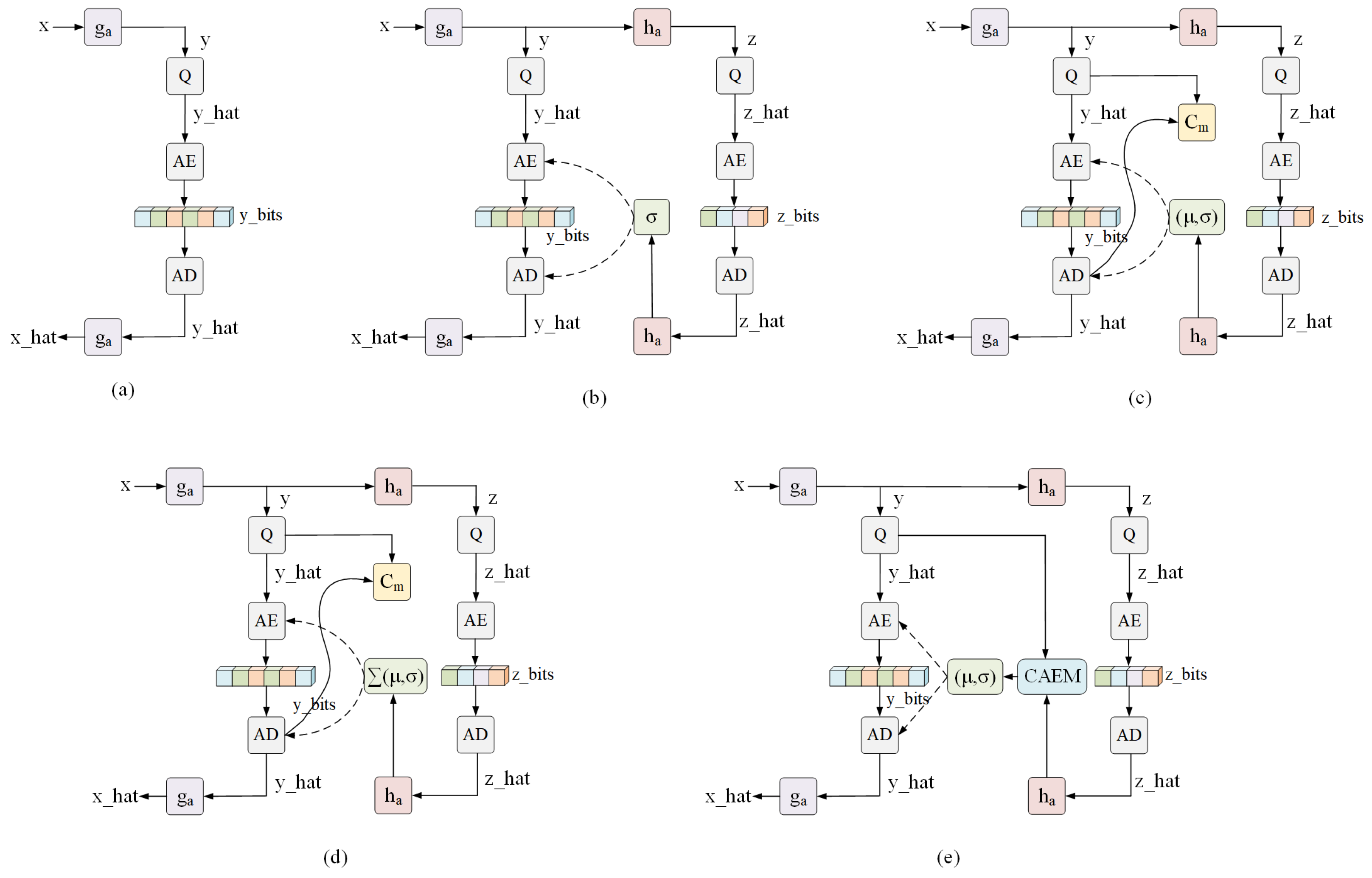
Learning-based approaches have become a prominent research focus. Compared to traditional techniques, these methods demonstrate superior performance in both compression efficiency and reconstruction quality. Ballé et al. [8] proposed an end-to-end image compression framework based on convolutional neural networks, as illustrated in Figure 1a. The encoder employs downsampling modules to convert the input image into high-dimensional latent representations, which reduces spatial redundancy among adjacent features.

To enhance the modeling capacity of the latent space, Ballé et al. [9] introduced a hyperprior network, as depicted in Figure 1b, which leverages side information derived from latent features to estimate their probability distribution and improves the precision of entropy coding. Building upon this foundation, Minnen et al. [10] proposed an enhanced framework that integrates an autoregressive context model within the hyperprior architecture, as shown in Figure 1c; by assuming a Gaussian distribution, the model jointly estimates the mean $\mu$ and variance $\sigma$ of the latent representation, which further refines the entropy modeling process. The incorporation of this context-aware mechanism enables more accurate probability estimation by effectively capturing local spatial dependencies.

In this context, Cheng et al. [11] introduced a discretized Gaussian mixture likelihood model aimed at enhancing the representation of latent distributions. This methodology demonstrates an improved balance between compression rate and reconstruction distortion, as depicted in Figure 1d.

To further enhance performance, Minnen et al. [12] introduced a channel-wise autoregressive entropy model that incorporates channel modulation and residual prediction within the latent space. This innovative approach not only enhances rate-distortion performance but also mitigates the sequential limitations associated with previous context-adaptive models, as illustrated in Figure 1e.

The Mamba architecture, which is grounded in a state space model (SSM) [13], has recently demonstrated considerable benefits in the management of long-sequence tasks. By employing a state transition technique, it effectively captures long-range interdependence while preserving linear computing complexity and exceptional scalability. This positions the Mamba architecture as a compelling alternative to models based on the Transformer framework. Furthermore, the introduction of selective scanning enhances the expressive capabilities of structured state space sequence models. The mechanism under scrutiny dynamically filters and concentrates on informative regions based on input features. This process significantly improves computational efficiency without compromising modeling accuracy.

Building on this foundation, VMamba [14] and Vim [15] extend the Mamba framework to two-dimensional vision tasks. By employing directionally selective scanning, these models efficiently capture and integrate global context. Consequently, they achieve broader receptive fields and enhanced performance in object detection and image classification, while also reducing inference latency and resource consumption. These features underscore their significant potential for visual understanding and practical application.

In this paper, we innovatively introduce the Mamba architecture into the field of remote sensing image compression, proposing a multi-scale channel global Mamba compression network (MGMNet). The objective is to achieve a better balance between compression performance and reconstruction. To this end, MGMNet has designed two core modules: the wavelet transform-guided local structure decoupling module (WTLS) and the channel–global information collaborative modeling module (CGIM).

In contrast to the intricate architecture and redundant parameters of the multi-branch high-low frequency compression model introduced by Xiang et al. [16], the WTLS module utilized in MGMNet adopts a wavelet decomposition strategy. This methodology segments the feature maps into multi-scale low-frequency and high-frequency sub-bands, facilitating the simultaneous modeling of global contours and local details within images. Building upon this framework, WTLS incorporates a local attention mechanism that prioritizes critical feature regions, such as edges, textures, and geometric structures present in the high-frequency sub-bands. This enhancement significantly improves the model’s ability to delineate essential features within visual data. In comparison to traditional multi-scale feature extraction methods that depend on deep convolutional stacking or extensive self-attention mechanisms, WTLS substantially reduces both the parameter count of the model and its computational requirements. This reduction allows for the effective capture of highly discriminative fine-grained features with diminished complexity, demonstrating notable structural compactness and computational efficiency.

Compared to the approach taken by Wang et al. [17], which relies solely on visual state space (VSS) scanning to obtain global semantics in the VMIC model, we find that during the compression of remote sensing images, pure bidirectional state scanning can establish long-term dependencies between pixels but has several limitations. First, VSS scanning utilizes uniform sampling and equal-weight processing, which poses difficulties in effectively capturing high-frequency details within the image. This results in decreased edge sharpness and a loss of detail after compression. Second, a single-state scan cannot differentiate the importance of various channels, which may lead to noise channels interfering with signal channels, compromising the quality of reconstruction. Lastly, remote sensing images exhibit significant spatial non-stationarity, with substantial differences in texture and statistical properties between adjacent areas. However, VSS scanning cannot adaptively prioritize the importance of spatial regions, preventing it from allocating more modeling resources to critical target areas (such as road edges and building structures) compared to background areas (such as vegetation and water bodies). Furthermore, a singular scanning mechanism encounters challenges in effectively managing the fusion of multi-scale information, which complicates the equilibrium between global semantics and local high-frequency responses. This limitation subsequently constrains the rate-distortion trade-off.

To address this challenge, we propose the CGIM module, which employs parallel execution of VSS scanning alongside a spatial–channel reconstruction weighting strategy. This module dynamically adjusts the importance of features and spatial positions for each channel, allowing the network to prioritize regions and frequency bands that are vital for enhancing compression efficiency and image fidelity. This methodology effectively mitigates the shortcomings associated with single scanning in capturing essential components. Furthermore, MGMNet capitalizes on the synergistic effects of the WTLS and CGIM modules to proficiently integrate multi-scale structural information with both global and local semantics in remote sensing images. It adeptly leverages critical regional features while maintaining a lightweight network architecture, ensuring ease of deployment and facilitating improved feature recovery and rate-distortion optimization.

The principal contributions of this article are outlined as follows:

• A novel lightweight remote sensing image compression network, designated as MGMNet, is introduced. This network combines the capabilities of state–space modeling with a collaborative modeling approach in channel space. Through the application of visual state–space modeling, a dynamic weighting mechanism for spatial channels has been developed. This mechanism allows the network to effectively capture the global semantic information present in remote sensing images, while simultaneously maintaining a precise focus on critical regions and significant edges. This approach achieves a superior compression-reconstruction trade-off under limited computational resources.
• A local structure modeling method based on wavelet transform has been developed, enabling the parallel modeling of low-frequency contours and high-frequency details in remote sensing images through multi-scale decomposition. When combined with a local attention strategy, this approach significantly enhances the representation of important details.
• To address the limitations of the visual state–space scanning mechanism in compression, we propose a dual-path modeling approach that integrates spatial–channel reconstruction strategies. This design preserves the capacity to model long dependencies but also effectively enhances the network’s responsiveness to high-frequency regions by dynamically weighting various channel features and spatial positions. This improvement leads to enhanced identification and reconstruction accuracy of target areas, significantly alleviating the shortcomings of single scanning in structural capture and multi-scale fusion.
• The experimental findings, encompassing rate-distortion performance and cross-validation, reveal that MGMNet exhibits considerable enhancements in performance relative to traditional image compression techniques as well as current learning-based methods across datasets. This robust evidence substantiates the efficacy of the proposed approach.

The organization of this article is delineated as follows: Section 2 provides a review of pertinent literature, whereas Section 3 presents the proposed MGMNet, elaborating on the theoretical underpinnings and operational functions of the WTLS and CGIM components. Section 4 outlines the experimental methodology and evaluation techniques employed, which will illustrate the efficacy and advantages of the proposed approach across various remote sensing datasets. Lastly, Section 5 encapsulates the article’s contributions and contemplates prospective avenues for future research.

2. Related Works

2.1. Deep Learning Compression Method Based on Natural Image

Expanding upon the work presented in [8], scholars have persistently advanced network architectures and probabilistic modeling techniques to augment the efficiency of compression. Guo et al. [18] introduced a dual-branch entropy model designed to independently capture causal context and global features to represent the latent space. Nevertheless, models based on convolutional neural networks (CNNs) generally depend on local convolutional operators, which constrain their capacity to effectively capture long dependencies. This shortcoming restricts their effectiveness in tasks with complex global structures, such as remote sensing image compression. Additionally, while context modeling techniques—such as autoregressive models [19,20]—can improve representation quality, they often suffer from sequential decoding, leading to high inference latency and limiting real-time deployment.

The constrained receptive field and lack of global representation in CNNs have motivated recent research to investigate Transformer architectures for image compression tasks. Khoshkhahtinat et al. [21] proposed a Transformer-based framework that combines nonlinear feature transformation with global modeling capabilities. This design suppresses spatial redundancy and enhances feature compactness. Zou et al. [22] developed a symmetric structure based on the Swin Transformer, incorporating hierarchical downsampling to improve multi-scale feature extraction. This approach achieves a balance between modeling power and computational efficiency. In addition, models such as GroupedMixer [23] enhance context modeling by introducing grouped processing and mixing operations, demonstrating the potential of Transformer-based architectures in image compression tasks. However, existing Transformer approaches still face challenges, including high architectural complexity and slow inference speeds. Moreover, most methods focus primarily on spatial modeling, while inter-channel dependencies remain underexplored.

2.2. Deep Learning Compression Method Based on Remote Sensing Image

Compared to natural images, remote sensing RGB imagery exhibits significant differences in scale, scene composition, and semantic distribution. It typically covers large geographical areas with diverse land cover types and pronounced scale variations. Such images often display strong regional homogeneity and spatial redundancy. Additionally, remote sensing data are frequently acquired from multiple platforms and across different periods, demonstrating temporal stability and repetition. These characteristics increase structural complexity and impose higher demands on the representation capacity and computational efficiency of compression models.

To leverage the spatiotemporal properties of remote sensing imagery, various compression strategies have been proposed. Zhang et al. [24] developed a Spatio-Temporal Context Model (STCM) that effectively captures both spatial neighborhoods and temporal sequences, while this model enhances compression performance, it necessitates high inter-frame consistency and precise registration, and its intricate architecture results in slow inference times. Li et al. [25] proposed the OF-RSIC method, which utilizes a Content-Weighted Attention Module (CWAM) to allocate bits more efficiently to significant regions, improving semantic fidelity. However, this enhancement is accompanied by a decline in quality in non-salient areas and an increase in computational demands. More recently, transformer-based models have been employed due to their superior capabilities in global modeling. Shi et al. [26] introduced MGSSNet, which combines convolutional neural networks (CNNs) and transformers through multi-head attention to improving spatial and spectral representation. Despite achieving enhanced accuracy, the model’s substantial parameter count and high inference costs impede its real-time application. Pan et al. [27] presented the CCGN model, which differentiates between structural and textural components to attain robust reconstruction performance at extremely low bitrates. Nonetheless, unstable training dynamics and a prolonged decoding pipeline limit its practical usability.

2.3. State Space Models

To balance modeling efficiency and global representation capacity, researchers have begun exploring the application of SSM in visual tasks. Originally developed for time-series analysis, SSMs have recently demonstrated strong long-range dependency modeling when integrated with deep learning frameworks. Gu et al. [13] proposed the Linear State Space Layer (LSSL) and Structured State Space (S4) model, significantly improving modeling. The Mamba architecture further advances this line of work by enabling linear scalability and fast inference, achieving strong performance across multimodal tasks. Liu et al. [14] introduced Mamba into vision by proposing VMamba, a visual SSM that enhances context modeling through two-dimensional state updates and selective scanning. Zhu et al. [15] proposed Vim, which employs a bidirectional state propagation mechanism to improve feature compression. For remote sensing scenarios, Ma et al. [28] designed RS3Mamba by incorporating a state-aware auxiliary branch to improve structural awareness. He et al. [29] proposed 3DSS-Mamba, which models spectral–spatial dependencies via three-dimensional state transitions, enhancing compression effectiveness. Zhao et al. [30] developed CNN-Mamba, which integrates spatial and spectral cues to improve multi-resolution image fusion.

In summary, although Transformer- and generation-based models have shown advancements in the accuracy of remote sensing image compression, their substantial architectural complexity and inference latency present considerable obstacles for practical deployment on edge devices. In contrast, State Space Models (SSMs) offer significant advantages, including structural simplicity, efficient inference processes, and strong capabilities for long-range modeling.

3. Proposed Method

This section offers a comprehensive overview of the proposed MGMNet and its associated components, which encompass the wavelet transform-guided local structure decoupling module (WTLS) and the channel–global information collaborative modeling module (CGIM).

3.1. Preliminaries

State Space Models (SSMs) [31], are a type of sequence model that can be considered as a linear time-invariant system commonly encountered in control theory, signal processing, or linear systems. SSM maps a one-dimensional continuous input signal $x\left(t\right)\in \mathbb{R}$ to an output response $y\left(t\right)\in \mathbb{R}$ through a learnable hidden state $h\left(t\right)\in {\mathbb{R}}^N$. This process can be represented using linear ordinary differential equations (ODEs), i.e.,

$$h^{\prime }\left(t\right)=\mathit{A}h\left(t\right)+\mathit{B}x\left(t\right)$$

(1)

$$y\left(t\right)=\mathit{C}h\left(t\right)$$

(2)

Equation (1) represents the state equation, and Equation (2) represents the observation equation. Where $h^{\prime }\left(t\right)\in {\mathbb{R}}^N$ is the derivative of $h\left(t\right)$ at the moment t, $\mathit{A}\in {\mathbb{R}}^{N\times N}$ is the state transition matrix, $\mathit{B}\in {\mathbb{R}}^{N\times 1}$ is the input matrix, and $\mathit{C}\in {\mathbb{R}}^{1\times N}$ is the output matrix.

Due to the challenges of integrating continuous SSM into deep learning models based on discrete sequences, the S4 [31] model serves as the discretized counterpart of continuous SSM, adapting them to deep learning frameworks by discretizing the ODEs. The Selective Scanning Space State Sequence Model (S6) [32] is also a discretized version of continuous SSM. To make continuous SSM suitable for discrete signals in image processing, a Zero-Order Holder (ZOH) [33] is used to convert continuous parameters $\mathit{A}$ and $\mathit{B}$ into discrete parameters $\overline{\mathit{A}}$ and $\overline{\mathit{B}}$, defined as follows:

$$\overline{\mathit{A}}=exp\left(\Delta \mathit{A}\right)$$

(3)

$$\overline{\mathit{B}}={\left(\Delta \mathit{A}\right)}^{-1}\left(exp\left(\Delta \mathit{A}\right)-\mathit{I}\right)·\Delta \mathit{B}$$

(4)

where $\Delta$ represents the time scale parameter, the discretized SSM can be expressed as follows:

$$h_t=\overline{\mathit{A}}{h}_{t-1}+\overline{\mathit{B}}{x}_t$$

(5)

$$y_t=\mathit{C}{h}_t$$

(6)

The output x can be computed through either global convolution or linear recurrence, defined as follows:

$$\overline{\mathit{K}}=\left(\mathit{C}\overline{\mathit{B}},\mathit{C}\overline{\mathit{AB}},\cdots ,\mathit{C}{\overline{\mathit{A}}}^{L-1}\overline{\mathit{B}}\right)$$

(7)

$$y=x\ast \overline{\mathit{K}}$$

(8)

where L is the length of the input sequence, $\overline{\mathit{K}}$ represents the structured convolutional kernel, and $\ast$ denotes the convolution operation.

3.2. Overall Framework

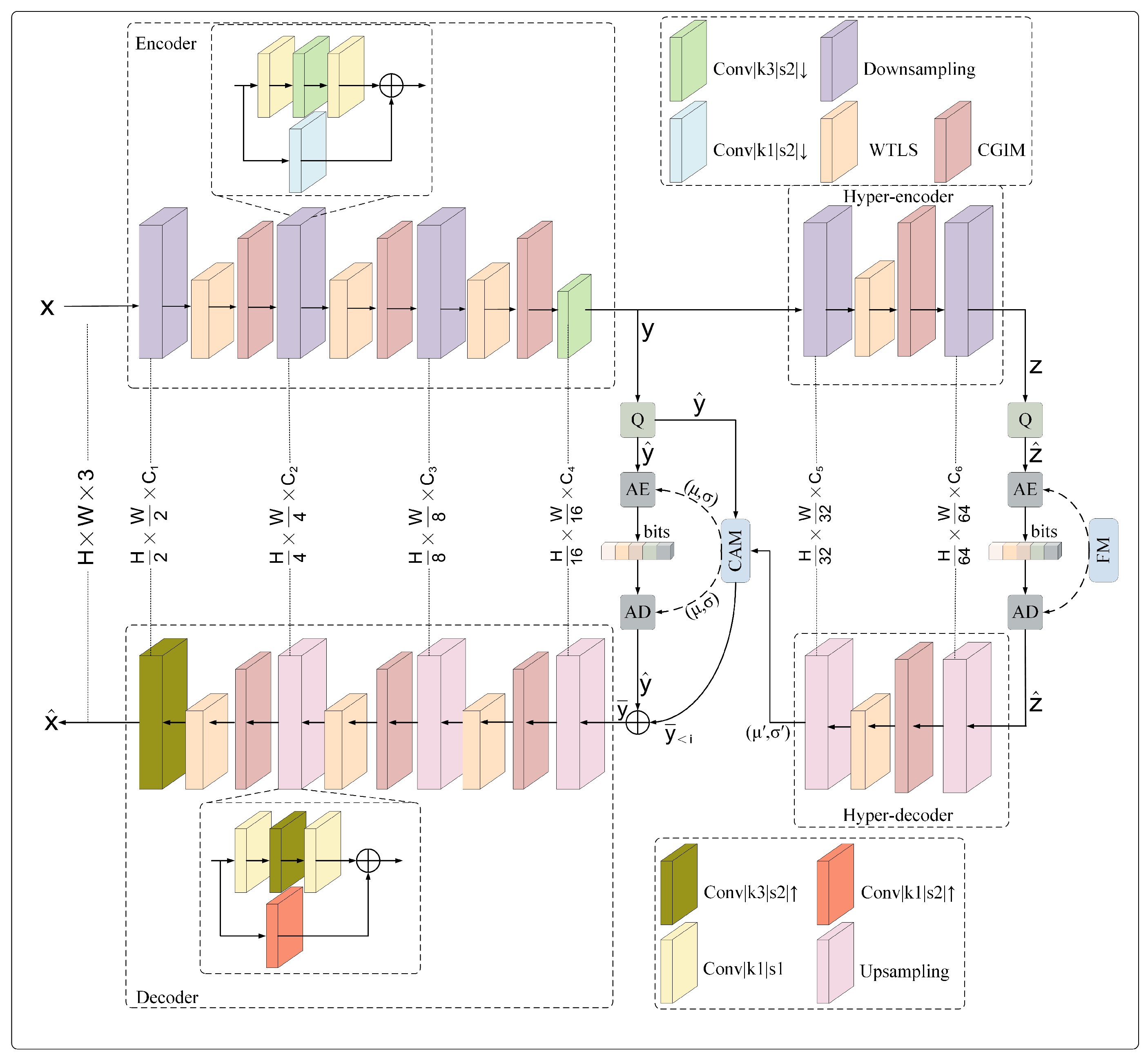
The overall architecture of MGMNet is illustrated in Figure 2. The network adopts a modular and scalable design tailored for remote sensing image compression, integrating spatial–frequency decoupling and global semantic modeling to enhance both compression efficiency and reconstruction fidelity.

The main encoder consists of down-sampling convolutions, followed by the WTLS and CGIM modules. WTLS is designed to decouple structural and textural components through wavelet-guided multi-scale analysis, while CGIM enhances global context understanding and channel-wise feature interaction. These two modules work collaboratively to provide a compact yet expressive latent representation of the input.

The decoder mirrors the encoder’s structure, incorporating the same functional modules to progressively reconstruct the image. This symmetrical design ensures consistency in spatial–frequency representation and contributes to high-quality restoration of fine details and large-scale structures.

The main encoding–decoding process adopts a three-stage encoding mechanism: The original input $\mathit{x}\in {\mathbb{R}}^{H\times W\times 3}$ is first transformed into a high-dimensional latent representation $\mathit{y}$ via the main encoder $g_a$. Subsequently, the latent features undergo discretization through the quantization module Q to produce the discretized latent features $\widehat{\mathit{y}}$. Finally, the quantized features $\widehat{\mathit{y}}$ are inversely mapped by the main decoder $g_s$ to generate the reconstructed image $\widehat{\mathit{x}}\in {\mathbb{R}}^{H\times W\times 3}$. This procedure can be mathematically formalized as follows:

$$\begin{array}{cc}\hfill \mathit{y}& =g_a\left(\mathit{x};\mathit{\varphi }\right)\hfill \\ \hfill \widehat{\mathit{y}}& =Q\left(\mathit{y}-\mathit{\mu }\right)+\mathit{\mu }\hfill \\ \hfill \widehat{\mathit{x}}& =g_s\left(\widehat{\mathit{y}};\mathit{\theta }\right)\hfill \end{array}$$

(9)

where $\mathit{x}$ and $\widehat{\mathit{x}}$ represent the original and reconstructed images, respectively, $\mathit{\varphi }$ and $\mathit{\theta }$ denote the trainable parameters of the main encoder $g_a$ and the main decoder $g_s$. $Q\left(·\right)$ represents the quantization operation.

This formulation enables MGMNet to perform compression and reconstruction of remote sensing images while achieving an effective balance among fidelity, compactness, and computational efficiency. Its modular architecture further facilitates seamless integration with components such as hyperprior entropy models and side information encoders, enhancing adaptability across diverse compression scenarios.

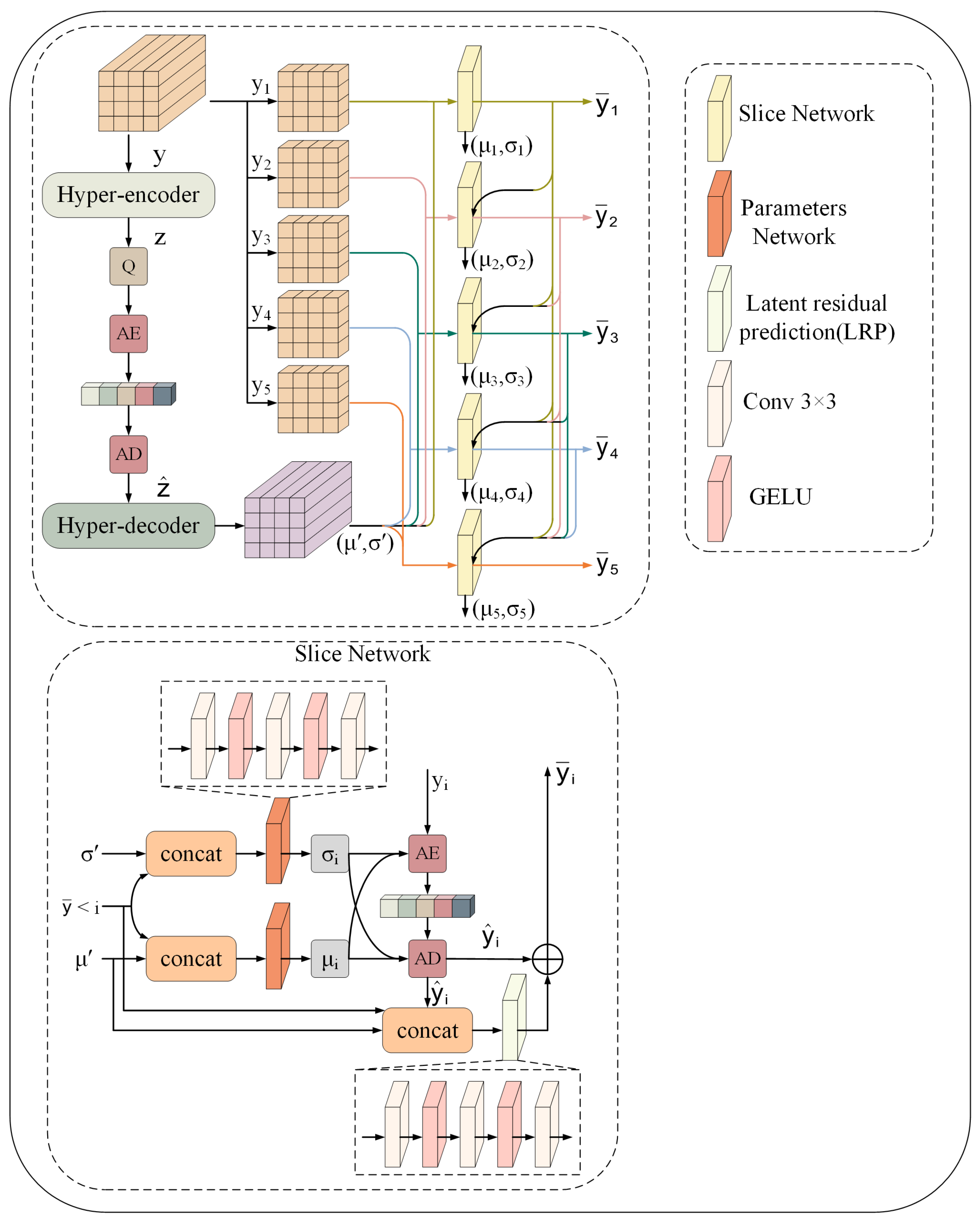
In the hyperprior framework, the main latent feature $\mathit{y}$ is first transformed into higher-order statistical features $\mathit{z}$ via the hyper-prior encoder $h_a$. After being discretized by the quantizer Q to yield $\mathit{z}$, the hyper-prior decoder $h_s$ decodes $\widehat{\mathit{z}}$ into the parameter required for entropy model.

Following previous studies [10,34,35], we round each $\left[\mathit{y}-\mathit{\mu }\right]$ and encode it into a bitstream rather than directly encoding $\mathit{y}$. The encoded symbol $\widehat{\mathit{y}}$ is then reconstructed as $\left[\mathit{y}-\mathit{\mu }\right]+\mathit{\mu }$. Subsequently, $\left[\mathit{y}-\mathit{\mu }\right]$ is losslessly encoded using a distance encoder, and its bitstream is represented by a single parameter $\mathit{\sigma }$. Utilizing the foundational concepts of channel-wise autoregressive entropy models, we partition the tensor $\mathit{y}$ into S separate segments. Each segment possesses dimensions of $W\times H\times {\displaystyle \frac{C}{S}}$, we set $S=5$ consistent with, [35]. The hyper-prior decoder decodes the side information in this framework to obtain two critical parameters, $\widehat{\mathit{\mu }}$ and $\widehat{\mathit{\sigma }}$. The entropy model functions in a sequential manner, determining the conditional probability distribution for each segment about the preceding segments. Each segment is subjected to entropy encoding and decoding processes, which facilitate the reconstruction of the comprehensive quantized latent representation $\widehat{\mathit{y}}$.

Subsequently, each slice ${\mathit{y}}_i$ is processed through the slicing network to obtain ${\overline{\mathit{y}}}_i$. A slice ${\overline{\mathit{y}}}_i$ can only be decoded after all preceding slices $\left\{{\overline{\mathit{y}}}_1,{\overline{\mathit{y}}}_2,\dots ,{\overline{\mathit{y}}}_{i-1}\right\}$ have been successfully decoded. Quantization operations inevitably introduce errors, which contribute to distortions in the reconstructed image. To mitigate these errors, we employ the rounding function and latent residual prediction $r_i$. Figure 3 illustrates the comprehensive methodology utilized in this entropy model.

3.3. Channel-Global Visual Model

Remote sensing images often encompass extensive geospatial features, such as urban areas, forests, and farmlands. Global features are crucial for compression models to understand the scene’s overall structure and help allocate bit resources more efficiently. In addition, remote sensing images exhibit strong correlations between different channels. Modeling channel features can effectively reduce redundant information and improve compression efficiency. However, efficiently extracting and integrating global and channel features to enhance compression performance remains a significant challenge.

The Visual State Space (VSS) model demonstrates proficiency in modeling long-range dependencies and capturing global features. Nonetheless, its fundamental component, the 2D-Selective Scanning (SS2D) module, exhibits certain limitations. SS2D begins by partitioning the image into patches of a fixed size, which are then analyzed along four diagonal orientations. Each patch matrix is subsequently flattened into a sequence for each orientation and processed for feature extraction. The results from all orientations are then integrated to amalgamate various global perspectives. Although this approach facilitates the incorporation of multi-directional context, the inflexible scanning order and patch-slicing methodology may constrain the model’s capacity to represent specific structured elements and local details effectively, while this mechanism is adept at global feature extraction, the absence of interaction among patches may lead to incomplete or distorted representations of global features that span multiple regions, such as river flows or mountain range extensions. Consequently, the SS2D module may struggle to establish effective connections between dispersed regions when identifying long-range features across various geographic units, increasing the likelihood of global information loss.

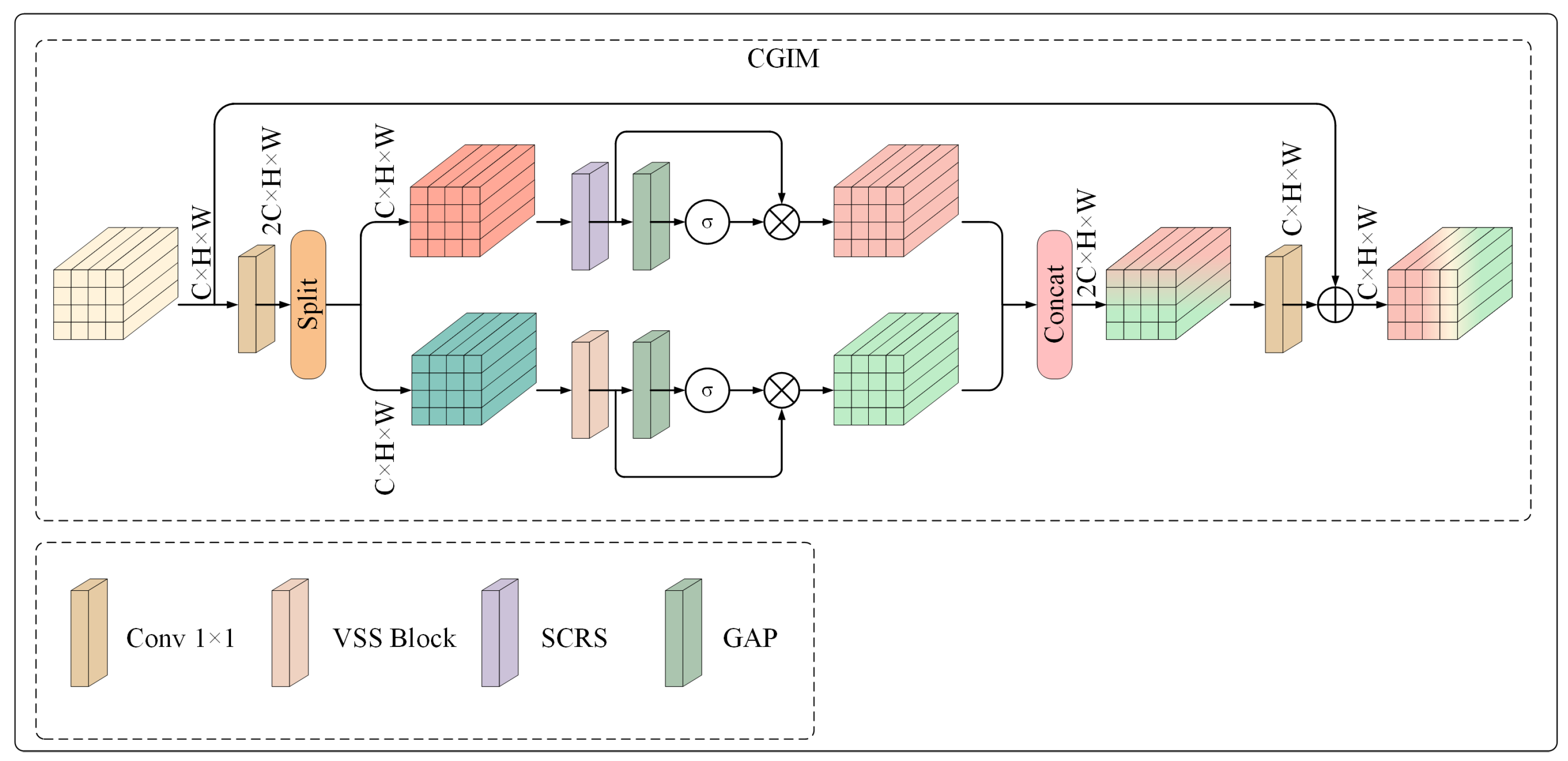
As depicted in Figure 4, we propose a channel–global information collaborative modeling module (CGIM) to tackle the aforementioned difficulties. The CGIM is a parallel architecture that includes the VSS model and the Spatial–Channel Reconstruction Strategy (SCRS) module. Among them, SCRS aims to extract more accurate global and channel information by optimizing spatial and channel features of remote sensing images. SCRS utilizes the synergy of spatial and channel dimensions to fuse the extracted global information with the channel information to complement the global feature extraction of VSS. This design can effectively mitigate the problem of information incompleteness that the SS2D module may cause. It ensures information integrity during compression and improves compression performance and reconstruction quality.

First, the tensor $X\in {\mathbb{R}}^{C\times H\times W}$ undergoes processing through a $1\times 1$ layer. This layer is configured to produce an output channel size of 2C. The output is then divided as $X_{VSS}\in {\mathbb{R}}^{C\times H\times W}$ and $X_{SCRS}\in {\mathbb{R}}^{C\times H\times W}$. It allows the VSS and SCRS modules to operate independently and in parallel. This parallel processing capability facilitates the more targeted and efficient extraction of features by each module, enhancing the overall representational capacity of the network.

Subsequently, the tensor $X_{VSS}$ is input into the VSS module, resulting in the output tensor $X_{VSS}^{\prime }$. Concurrently, the tensor $X_{SCRS}$ is processed through the SCRS module to yield the output tensor $X_{SCRS}^{\prime }$. Subsequently, the tensor $X_{VSS}^{\prime }$ is processed through a global average pooling (GAP) layer. Following the application of a sigmoid function, the output generated by the GAP layer is multiplied by the tensor $X_{VSS}^{\prime }$, resulting in the tensor $X_{VSS}^{″}$. Similarly, $X_{SCRS}^{\prime }$ undergoes the same process, resulting in $X_{SCRS}^{″}$. The tensors $X_{VSS}^{″}$ and $X_{SCRS}^{″}$ are concatenated. Subsequently, the features extracted by the VSS and SCRS modules are integrated through a second $1\times 1$ layer. The output channel size of this convolutional layer is C. Ultimately, the input features X are incorporated with the output features to produce the final output $X_{out}$. This process can be mathematically represented as follows:

$$\begin{array}{cc}\hfill X_{VSS},X_{SCRS}& =Split\left(Con{v}_{1\times 1}\left(X\right)\right)\hfill \\ \hfill X_{VSS}^{\prime }& =VSS\left(X_{VSS}\right)\hfill \\ \hfill X_{SCRS}^{\prime }& =SCRS\left(X_{SCRS}\right)\hfill \\ \hfill X_{VSS}^{″}& =\sigma \left(GAP\left(X_{VSS}^{\prime }\right)\right)\times X_{VSS}^{\prime }\hfill \\ \hfill X_{SCRS}^{″}& =\sigma \left(GAP\left(X_{SCRS}^{\prime }\right)\right)\times X_{SCRS}^{\prime }\hfill \\ \hfill X_{out}& =Con{v}_{1\times 1}\left(Concat\left(X_{VSS}^{″},X_{SCRS}^{″}\right)\right)+X\hfill \end{array}$$

(10)

where $Split\left(•\right)$ denotes the split operation. $\sigma \left(•\right)$ signifies the Sigmoid function.

3.3.1. Visual State Space Model

The VSS model, derived from VMamba [14], is a core component of CGIM. Given an input feature $X_{in}\in {\mathbb{R}}^{C\times H\times W}$, it is first processed through Layer Normalization (LN) before being routed to two gated branches. In the first branch, the input undergoes a linear layer, depthwise separable convolution, and SiLU activation function [36] for feature extraction. The extracted features are fed into the SS2D module to capture global features and establish long-range dependencies. Finally, the output passes through a second LN layer to produce the first branch output $X_{out1}$. This process can be represented as follows:

$$\begin{array}{c}\hfill X_{out1}=L{N}_2\left(SS2D\left(SiLU\left(DWConv\left(Linea{r}_1\left(L{N}_1\left(X_{in}\right)\right)\right)\right)\right)\right)\end{array}$$

(11)

In the second branch, the input goes through a linear layer and SiLU activation function to get the output of the second branch $X_{out2}$. It can be expressed as follows:

$$\begin{array}{c}\hfill X_{out2}=SiLU\left(Linea{r}_2\left(L{N}_1\left(X_{in}\right)\right)\right)\end{array}$$

(12)

The outputs $X_{out1}$ and $X_{out2}$ are fused to integrate features from both branches through element-wise multiplication. A linear layer is applied to enhance feature integration further. Finally, a skip connection is established between the linear layer’s output and the input $X_{in}$, resulting in the final output $X_{VSS\_out}$ of the VSS module. This process can be represented as follows:

$$\begin{array}{c}\hfill X_{VSS\_out}=Linear\left(X_{out1}\odot X_{out2}\right)+X_{in}\end{array}$$

(13)

where ⊙ denotes element-wise multiplication.

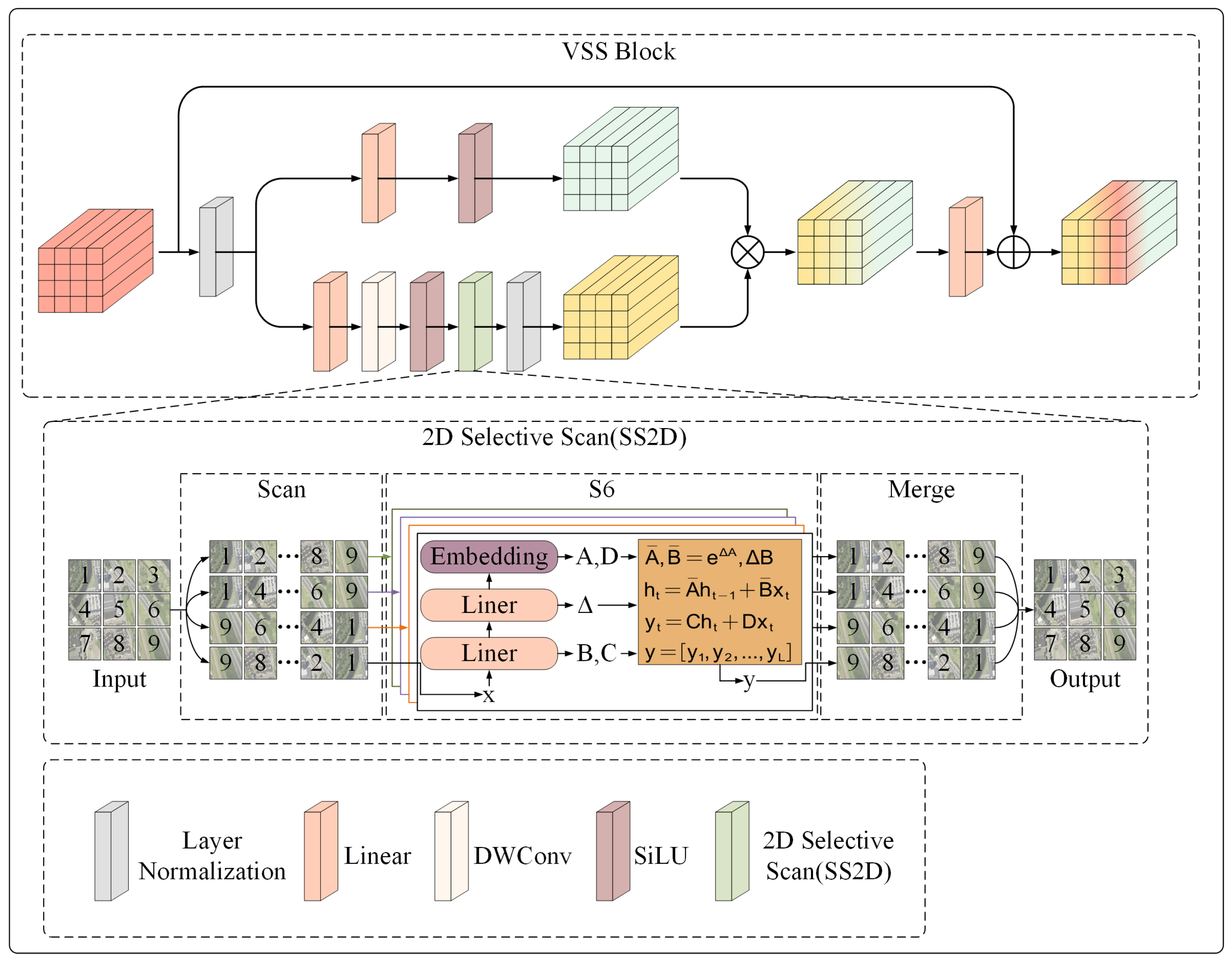
As illustrated in Figure 5, the SS2D module processes data in three steps: cross-scanning, selective scanning using S6 blocks, and cross-merging. Given an input feature map X, it is first divided into patches of equal size. The SS2D module then performs cross-scanning in four directions (top-left to bottom-right, bottom-right to top-left, top-right to bottom-left, and bottom-left to top-right) to unfold the input patches into four independent sequences. Each sequence is processed in parallel using the S6 block selective scanning mechanism, which ensures comprehensive feature extraction in all directions.

Finally, a cross-merging operation combines the sequences from all directions, reconstructing the output feature map $\overline{X}$ with the exact dimensions as the input. This process is expressed as follows:

$$\begin{array}{cc}\hfill X_v& =\mathrm{scan}\left(X,v\right)\hfill \\ \hfill {\overline{X}}_v& =\mathrm{S}6\left(X_v\right)\hfill \\ \hfill \overline{X}& =\mathrm{merge}\left({\overline{X}}_1,{\overline{X}}_2,{\overline{X}}_3,{\overline{X}}_4\right)\hfill \end{array}$$

(14)

where $v\in \left[1,2,3,4\right]$ denotes four different scanning directions, $scan\left(•\right)$ and $merge\left(•\right)$ denote the cross-scan and cross-merge operations.

The S6 model [32], is an enhanced version built upon the S4 model [31], with its core innovation being the introduction of a selective mechanism that enables the model to dynamically adjust the parameter configurations of the State Space Model (SSM) based on the input content. This mechanism endows the model with improved adaptability and selective processing capability, allowing it to retain critical semantic information while effectively filtering out redundant or irrelevant details during feature extraction. As a result, the model achieves better representational efficiency and reconstruction quality.

In terms of architectural design, S6 also adopts the Spatial-Sequential 2D (SS2D) framework, which encodes images through complementary one-dimensional sequential traversal paths (e.g., row-wise and column-wise), enabling each pixel to aggregate spatial context from multiple directions. This design effectively constructs a global receptive field in the 2D space, significantly enhancing the model’s ability to capture long-range dependencies and cross-region structural patterns.

The selective mechanism introduced in the S6 model makes it particularly well-suited for handling the spatial non-stationarity commonly found in remote sensing images. Such images often contain rich and diverse land-cover types, with significant variations in texture density, structural scale, and edge sharpness across regions, leading to high spatial heterogeneity. Traditional static modeling approaches often lack the flexibility to adapt to this heterogeneous distribution, resulting in the loss of structural information or the inclusion of excessive redundant features.

In S6, the selective state modulation mechanism performs input-driven dynamic parameter adjustment, enabling differentiated state update behaviors across spatial regions. In areas with complex textures or abrupt structural changes, the model enhances state retention and feature fusion to better capture fine details and boundaries. Conversely, in flat, highly repetitive, or information-sparse regions, it suppresses state updates and actively “forgets” redundant content, thereby improving overall modeling efficiency. This mechanism effectively constructs a form of spatially selective memory, allowing the model to adaptively shift its “attention focus” in response to diverse spatial structures, thus improving its capacity to handle the complex and dynamic spatial patterns in remote sensing imagery.

Through the synergistic integration of the selective mechanism and the SS2D framework, the S6 model exhibits not only strong global modeling capabilities and efficient sequential processing but also the flexibility to adapt its modeling strategies based on spatial characteristics of the input, demonstrating excellent performance in non-stationary environments.

3.3.2. Spatial–Channel Reconstruction Strategy

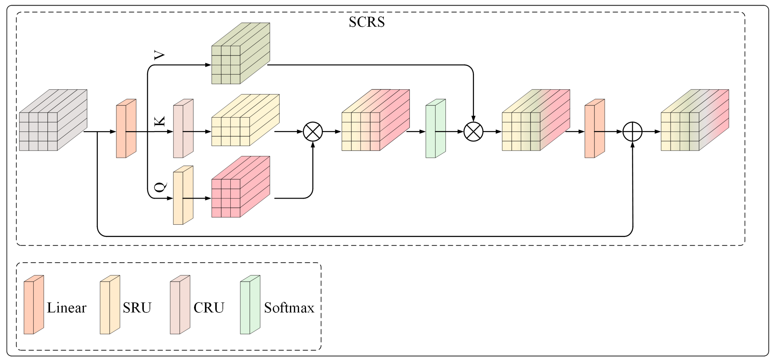
The Spatial–Channel Reconstruction Strategy (SCRS) represents an enhancement of the SCConv architecture initially proposed by Li et al. [37]. This strategy enhances visual representation through the implementation of a dual-path mechanism, which adeptly decouples and simultaneously models spatial and channel features. This is illustrated in Figure 6.

The Spatial Reconstruction Unit (SRU) employs a separation–reconstruction methodology to mitigate spatial redundancy and improve spatial feature representation. Concurrently, the Channel Reconstruction Unit (CRU) utilizes a separation–transformation–fusion approach to diminish channel redundancy and augment inter-channel correlations. The outputs generated by SRU and CRU are combined through element multiplication to effectively merge spatial and channel information. Attention weights are computed through a Softmax function and applied to V. A linear transformation follows to strengthen feature interactions.

By separating spatial and channel dependencies, this architecture facilitates enhanced modeling of global–local attention and augments the discriminative power of the features obtained. The following presents a streamlined mathematical formulation:

$$\begin{array}{cc}\hfill Q,K,V& =Linea{r}_1\left(X_{att}\right)\hfill \\ \hfill Q_{SRU}& =SRU\left(Q\right)\hfill \\ \hfill K_{CRU}& =CRU\left(K\right)\hfill \\ \hfill X_{SCRS\_out}& =Linea{r}_2\left(SoftMax\left(Q_{SRU}{K}_{CRU}^T/\sqrt{d}\right)V\right)\hfill \end{array}$$

(15)

where d denotes the dimension of input.

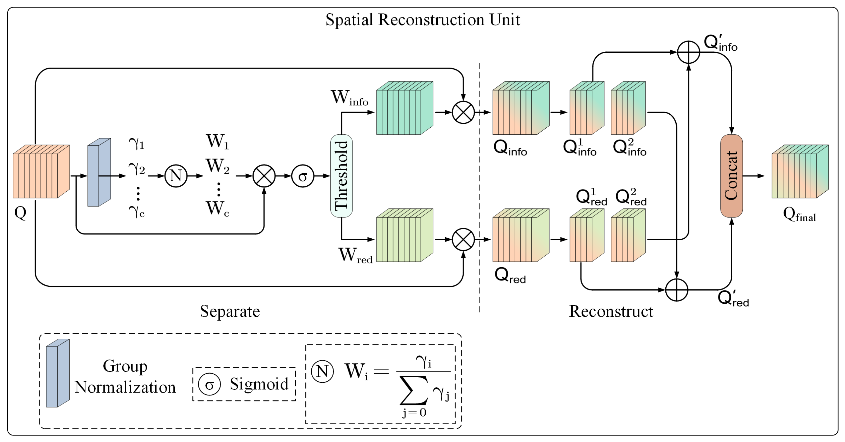
3.3.3. Spatial Reconstruction Unit

As illustrated in Figure 7, the Spatial Reconstruction Unit (SRU) refines feature maps by reducing spatial redundancy through a “separate-and-reconstruct” approach.

The input tensor $Q\in {\mathbb{R}}^{C\times H\times W}$ is normalized via Group Normalization; the resulting scaling coefficients serve as indicators of evaluating each channel’s content. This process is mathematically represented as follows:

$$\begin{array}{c}\hfill X_{out}=GN\left(Q\right)=\gamma {\displaystyle \frac{Q-\mu }{\sqrt{{\sigma }^2+\epsilon }}}+\beta \end{array}$$

(16)

where the parameters $\gamma$ and $\beta$ are adjustable affine transformation coefficients within the GN layer. Feature maps possessing abundant spatial information generally demonstrate more spatial pixel fluctuations, resulting in bigger corresponding $\gamma$ values. This relationship can be articulated mathematically as follows:

$$\begin{array}{c}\hfill W_{\gamma }=\left\{w_i\right\}={\displaystyle \frac{{\gamma }_i}{{\sum }_{j=1}^C{\gamma }_j}},i,j=1,2,\dots ,C.\end{array}$$

(17)

In this context, $W_{\gamma }$ represents the normalized weight employed to indicate the significance of various feature maps. An increase in the value of $\gamma$ suggests a greater diversity and richness of spatial information present within the feature maps.

First, the Sigmoid function is employed to normalize the weights $W_{\gamma }$. Subsequently, these weights are classified using a gating threshold of 0.5. Informative weights $W_{info}$ are represented by 1 for weights that exceed the threshold, while non-informative weights $W_{red}$ are represented by 0 for weights that are below the threshold. This process can be expressed as follows:

$$\begin{array}{c}\hfill W_{info},W_{red}=Gate\left(Sigmoid\left(W_{\gamma }\left(GN\left(Q\right)\right)\right)\right)\end{array}$$

(18)

Subsequently, the input feature Q is subjected to multiplication by the informative weight $W_{info}$ and the non-informative weight $W_{red}$, yielding two distinct weighted features: $Q_{info}$ and $Q_{red}$. The feature $Q_{info}$ encapsulates critical attributes characterized by a higher information content, whereas $Q_{red}$ encompasses redundant attributes with comparatively lower information content. These two weighted features are then amalgamated through a cross-reconstruction operation, which culminates in the generation of enhanced features $Q_{info}^{\prime }$ and $Q_{red}^{\prime }$ that exhibit diminished spatial redundancy. The cross-reconstruction process effectively synthesizes the two weighted features, augmenting their information flow. Ultimately, $Q_{info}^{\prime }$ and $Q_{red}^{\prime }$ are concatenated to produce the final spatially refined feature $Q_{final}$. The mathematical representation of the reconstruction process can be articulated as follows:

$$\begin{array}{cc}\hfill Q_{info}& =W_{info}\otimes Q\hfill \\ \hfill Q_{red}& =W_{red}\otimes Q\hfill \\ \hfill Q_{info}^{\prime }& =Q_{info}^1\oplus Q_{red}^2\hfill \\ \hfill Q_{red}^{\prime }& =Q_{info}^2\oplus Q_{red}^1\hfill \\ \hfill Q_{final}& =Concat\left(Q_{info}^{\prime },Q_{red}^{\prime }\right)\hfill \end{array}$$

(19)

The symbol ⊗ signifies element-wise multiplication. The symbol ⊕ denotes element-wise addition.

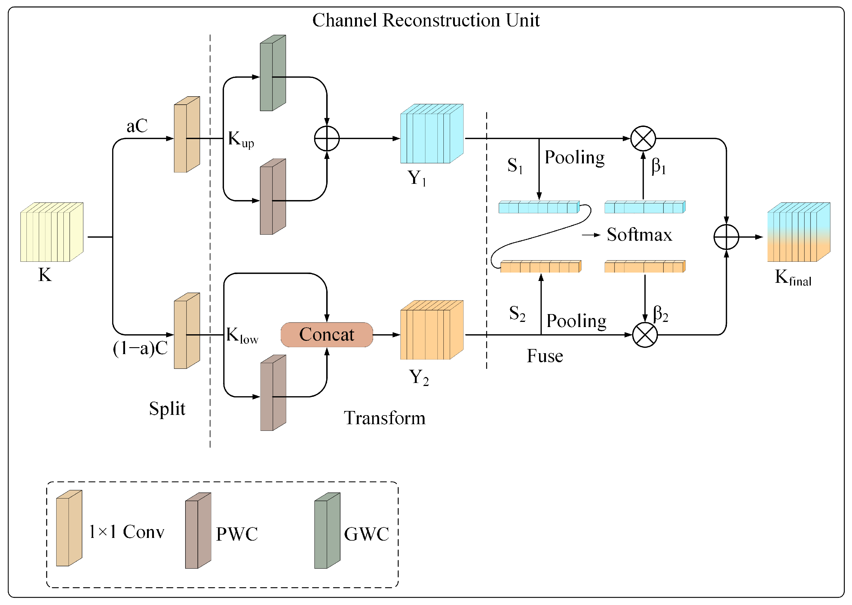
3.3.4. Channel Reconstruction Unit

To better leverage redundant information across channels, we introduce the Channel Reconstruction Unit (CRU), which refines feature channels to extract more discriminative channel features. As illustrated in Figure 8, the CRU adopts a “separation–transformation-fusion” strategy to reduce channel redundancy and enhance feature representation capacity effectively.

Separation. The input feature $K\in {\mathbb{R}}^{C\times H\times W}$ is first split along the channel dimension. It is divided into two parts: one with $\alpha C$ channels and the other with $\left(1-\alpha \right)C$ channels. Here, $0⩽\alpha ⩽1$ represents the channel split ratio. Each sub-feature is then processed by a 1×1 convolution. This operation compresses the channels and reduces the computational costs. As a result, the original feature K is separated into an upper part $K_{up}$ and a lower part $K_{low}$. These two parts serve as the basis for subsequent transformation and fusion operations.

Transformation. During the transformation phase, the input feature $K_{up}$ undergoes processing through a specialized rich feature extraction module. This module integrates Group Convolution (GWC) and Pointwise Convolution (PWC) to derive more representative high-level features while ensuring computational efficiency. Nonetheless, the segmentation of channels into distinct groups may restrict inter-channel communication. PWC introduces fully connected operations across channels to address this limitation and enhance inter-feature interactions. The outputs generated by the GWC and PWC are subsequently combined through element-wise addition to yield the aggregated feature map $Y_1$. This transformation can be articulated as follows:

$$\begin{array}{c}\hfill Y_1=M^G{K}_{up}+M^{P_1}{K}_{up}\end{array}$$

(20)

where $M^G$ denotes the learnable weight matrix for GWC. $M^{P_1}$ denotes the learnable weight matrix for PWC.

During the lower transformation stage, the variable $K_{low}$ is processed through a PWC module, which is responsible for extracting shallow detail features that complement the high-level features derived from the upper transformation stage. The output generated by the PWC module is subsequently combined with the original $K_{low}$ through a channel-wise concatenation operation. This procedure results in the final output feature of the lower transformation stage, referred to as $Y_2$. The entire process can be mathematically represented as follows:

$$\begin{array}{c}\hfill Y_2=Concat\left(M^{P_2}{K}_{low},K_{low}\right)\end{array}$$

(21)

where $M^{P_2}$ denotes the learnable weight matrix for PWC.

Fusion. The transformed output features $Y_1$ and $Y_2$ are adaptively integrated utilizing a streamlined SKNet [38] approach. At the outset, GAP is employed to consolidate input feature information using the channel statistics $S_m$.

The channel descriptors corresponding to the upper and lower transformation features, denoted as $S_1$ and $S_2$, are subsequently combined. The vectors ${\beta }_1$ and ${\beta }_2$ are produced through the application of a channel-wise soft attention mechanism, executed as follows:

$$\begin{array}{c}\hfill {\beta }_1={\displaystyle \frac{e^{S_1}}{e^{S_1}+e^{S_2}}},{\beta }_2={\displaystyle \frac{e^{S_2}}{e^{S_1}+e^{S_2}}},{\beta }_1+{\beta }_2=1\end{array}$$

(22)

In the concluding phase, the feature importance vectors ${\beta }_1$ and ${\beta }_2$ facilitate the integration of $Y_1$ and $Y_2$ within the channel dimension. This results in the final channel-refined feature $K_{final}$, as follows:

$$\begin{array}{c}\hfill K_{final}={\beta }_1{Y}_1+{\beta }_2{Y}_2\end{array}$$

(23)

The CRU leverages lightweight convolutional operations to capture informative channel-level features. At the same time, it applies a cost-efficient feature reuse mechanism to mitigate redundancy. This design improves both computational efficiency and feature representation quality.

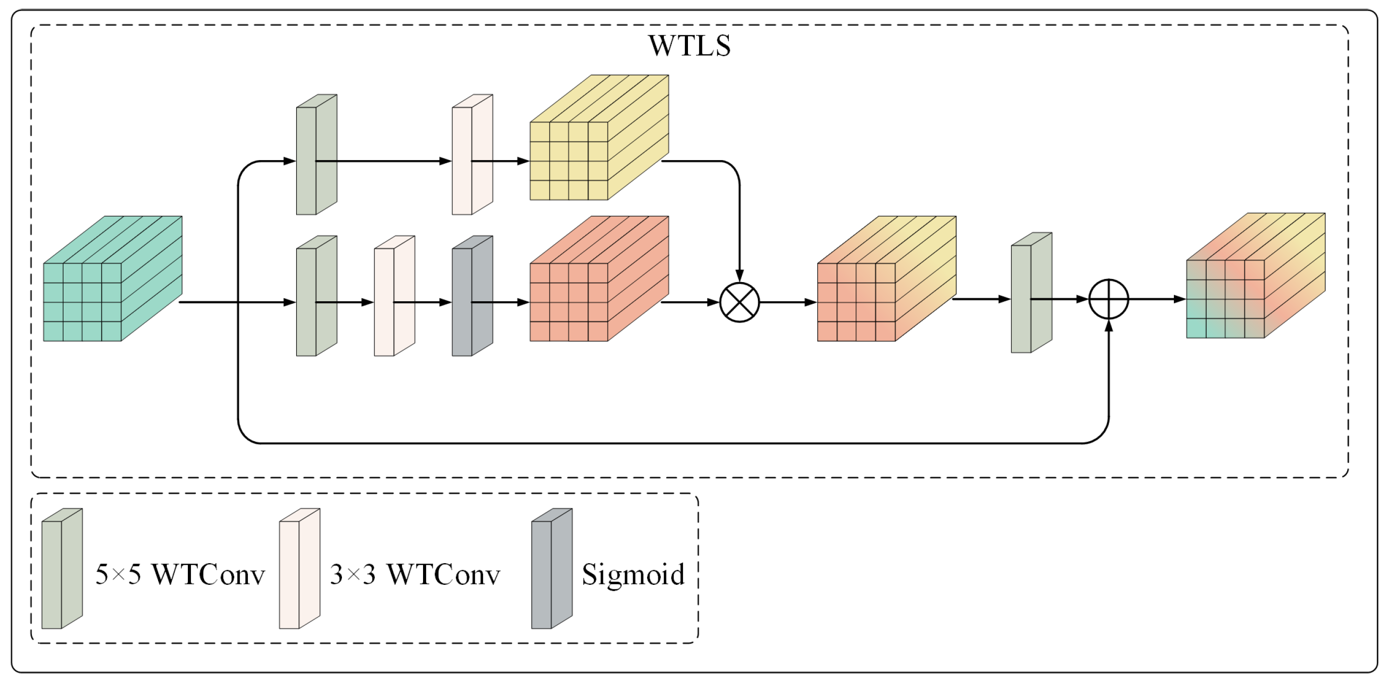
3.4. Wavelet Transform-Guided Local Structure Decoupling Module

Remote sensing images typically encompass intricate details, such as the edges of roads and buildings, making the efficient extraction of local features essential for maintaining critical information and enhancing the quality of image reconstruction. Traditional convolutional neural networks (CNNs) often encounter challenges in capturing long-range dependencies due to their limited receptive fields. This limitation can lead to inadequate contextual awareness and suboptimal feature representation. Furthermore, the constrained receptive field hinders conventional CNNs from effectively capturing large-scale features and long-range dependencies among distant pixels. Consequently, pertinent information that is spatially distant may not be adequately integrated into local features, adversely impacting both compression performance and reconstruction quality.

We propose a wavelet transform-guided local structure decoupling module (WTLS) based on wavelet transform convolution [39] to efficiently extract multi-scale local features from feature maps to address the aforementioned issues. Specifically, wavelet transform convolution leverages the multi-scale decomposition properties of the wavelet transform to enlarge the receptive field while avoiding excessive parameterization significantly. In contrast to conventional convolutions, wavelet transform convolution offers a significant advantage in the extraction of low-frequency information, as wavelet transforms emphasize low-frequency components during the decomposition process. The integration of wavelet transform convolution within the WTLS model facilitates a more precise extraction of multi-scale local features while preserving large-scale contextual information. This capability substantially contributes to the improvement of remote sensing image compression performance and the quality of reconstruction.

As shown in Figure 9, the input feature is first processed by the initial branch. This branch consists of a $5\times 5$ wavelet convolution (WTConv), followed by a $3\times 3$ WTConv. Both layers contribute to multi-scale feature extraction in the wavelet domain. The output of the $3\times 3\mathrm{WTConv}$ is then mapped to result in the output $X_1\in {\mathbb{R}}^{C\times H\times W}$ of the first branch.

Subsequently, the input feature is directed through the second branch of the model. This branch systematically applies a $5\times 5\mathrm{WTConv}$ followed by a $3\times 3\mathrm{WTConv}$. The resultant feature is represented as $X_2\in {\mathbb{R}}^{C\times H\times W}$. An element-wise multiplication is then executed between $X_1$ and $X_2$ to enhance the interaction of the features. The resulting product undergoes further refinement through a $5\times 5\mathrm{WTConv}$ to augment the fusion process. Ultimately, the output of this convolution is combined with the original input X, yielding the final output denoted as $X_{WTLS\_out}$. The entire process can be mathematically expressed as follows:

$$\begin{array}{cc}\hfill X_1& =Sigmoid\left({\mathrm{WTConv}}_{3\times 3}\left({\mathrm{WTConv}}_{5\times 5}\left(X\right)\right)\right)\hfill \\ \hfill X_2& ={\mathrm{WTConv}}_{3\times 3}\left({\mathrm{WTConv}}_{5\times 5}\left(X\right)\right)\hfill \\ \hfill X_{WTLS\_out}& ={\mathrm{WTConv}}_{5\times 5}\left(X_1\otimes X_2\right)+X\hfill \end{array}$$

(24)

where ⊗ denotes element-wise multiplication.

4. Experiments

To ensure a comprehensive evaluation of MGMNet, we employed DOTA, UC-Merced, and NWPU-RESISC45 datasets, which encompass diverse and abundant ground object features, making them well-suited for validating the model’s effectiveness.

MGMNet is compared with several classical image compression standards, including JPEG2000 [5], WebP [7], BPG, and AVIF. In addition, we included recent learning-based approaches, such as those proposed by Cheng et al. [11] (Cheng2020), Jiang et al. [40] (Jiang2022), Liu et al. [34] (Liu2023), Liu et al. [41] (Liu2024), and Qin et al. [42] (Qin2024). Quantitative analyses utilizing four evaluation indicators indicate that MGMNet consistently outperforms its competitors across all metrics.

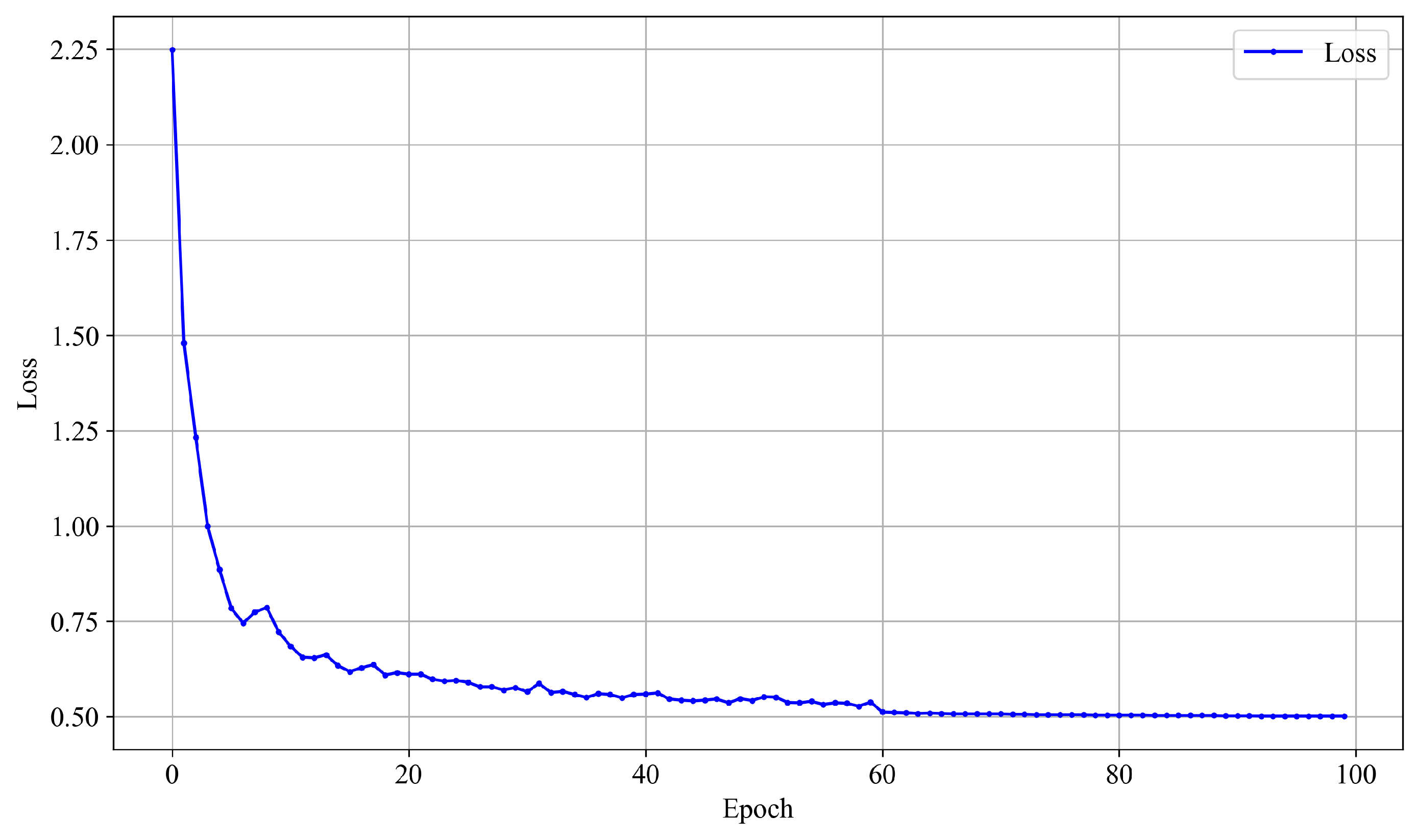
4.1. Loss Fuction

The loss function of our model consists of two components. The first component constrains the bitrate of the bitstream generated during the compression process, including the latent representation and side information. The second component measures the mean squared error (MSE) between the input image and the final output of the model. The formulation is as follows:

$$\begin{array}{cc}\hfill \mathrm{L}& =\mathrm{R}+\lambda ·\mathrm{D}\hfill \\ \hfill & ={\mathbb{E}}_{x\sim p_x}[-{log}_2{p}_{\widehat{y}}\left(Q\left(y\right)\right)]\hfill \\ \hfill & +{\mathbb{E}}_{x\sim p_x}[-{log}_2{p}_{\widehat{z}}\left(\widehat{z}\right)]+\lambda ·{\mathbb{E}}_{x\sim p_x}\left[d(x,\widehat{x})\right]\hfill \end{array}$$

(25)

The rate-distortion optimization aims to simultaneously reduce the size of the compressed bitstream and the distortion in the decompressed image. This process can be summarized as minimizing the number of bits required for compression while maintaining the quality of the decoded image.

To illustrate this, we take the UC-Merced dataset as an example and present the training process under the setting of $\lambda$ = 0.0035 (corresponding to bpp = 0.46). Figure 10 shows the trend of the loss function concerning the number of training epochs.

As observed from the figure, the model exhibits a fast convergence behavior at the early stages of training under this $\lambda$ setting. The overall training process remains stable, with a smooth and steady decrease in the loss. Therefore, under this configuration, the model achieves performance saturation before reaching the preset 150 epochs. Early stopping can thus effectively reduce computational cost while mitigating the risk of overfitting.

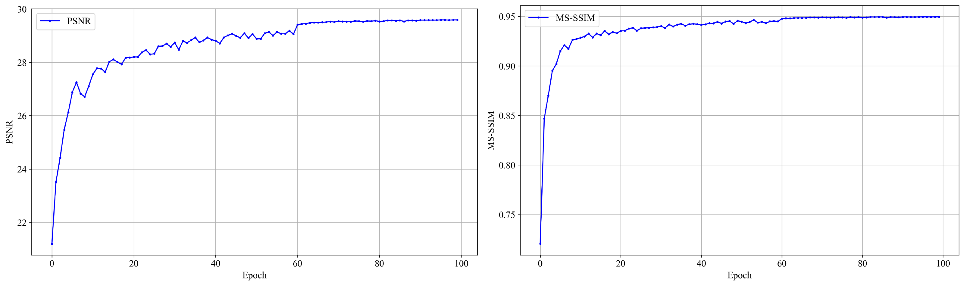
Similarly, under the current setting of $\lambda$ = 0.0035, we further illustrate the evolution of two image quality evaluation metrics, PSNR and MS-SSIM, during training. As shown in Figure 11, both metrics exhibit a steady upward trend as the number of epochs increases and gradually converges in the later stages of training. This indicates that the model continuously improves its reconstruction quality while maintaining strong compression performance.

In particular, around epoch 100, both PSNR and MS-SSIM curves begin to stabilize, suggesting that the model has reached a performance saturation point, where further training yields marginal improvements. Therefore, under this $\lambda$ configuration, early termination of training does not compromise the final model performance and helps improve training efficiency while reducing computational resource consumption.

4.2. Experimental Settings

All learning-based models are developed using the PyTorch 2.1.0. framework. Training is conducted on an NVIDIA RTX 3090 GPU. The Adam optimizer [43] is employed to perform gradient-based optimization. During training, image patches of 256 × 256 pixels are uniformly and randomly sampled from the training datasets. The training process begins with a learning rate of 1 $\times {10}^{-4}$. A mini-batch size of 8 is used during optimization. The model is trained for a total of 200 epochs. The learning rate is gradually reduced during training. It is set to ${10}^{-5}$ after 100 epochs, and further lowered to ${10}^{-6}$ at epoch 150. At epoch 180, it is decreased to ${10}^{-7}$, which is then kept constant until training completes.

The model is trained using a rate-distortion loss function. Distortion is quantified by the MSE between the original and reconstructed images. The balance between rate and distortion is controlled by a trade-off parameter $\lambda$. We evaluate the model under different compression levels by varying $\lambda$ within the set [0.0018, 0.0035, 0.0067, 0.013, 0.025, 0.05].

4.3. Evaluation Indicators

Bit rate is quantified in terms of bits per pixel (Bpp). The assessment of image quality is conducted through four complementary metrics, which are encapsulated in rate-distortion (R-D) curves.

PSNR (Peak Signal-to-Noise Ratio) quantifies the pixel-level reconstruction error, with elevated values signifying enhanced fidelity.

MS-SSIM (Multi-Scale Structural Similarity Index) examines structural similarity across various scales, where increased values imply superior perceptual quality.

LPIPS (Learned Perceptual Image Patch Similarity) assesses perceptual similarity through deep feature representations, with reduced values reflecting greater visual similarity.

VIFp: Quantifies the amount of visual information preserved; higher values denote better quality.

4.4. Analysis of Wavelet Basis and Convolution Kernel Size in WTLS Module

The WTLS (wavelet transform-guided local structure decoupling module) plays a critical role in balancing spatial–frequency representation and computational efficiency in the proposed compression framework. To systematically evaluate the influence of key architectural components, we investigate two primary factors: the choice of wavelet basis and the convolution kernel size, which, respectively, control the frequency decomposition and the spatial receptive field of the model.

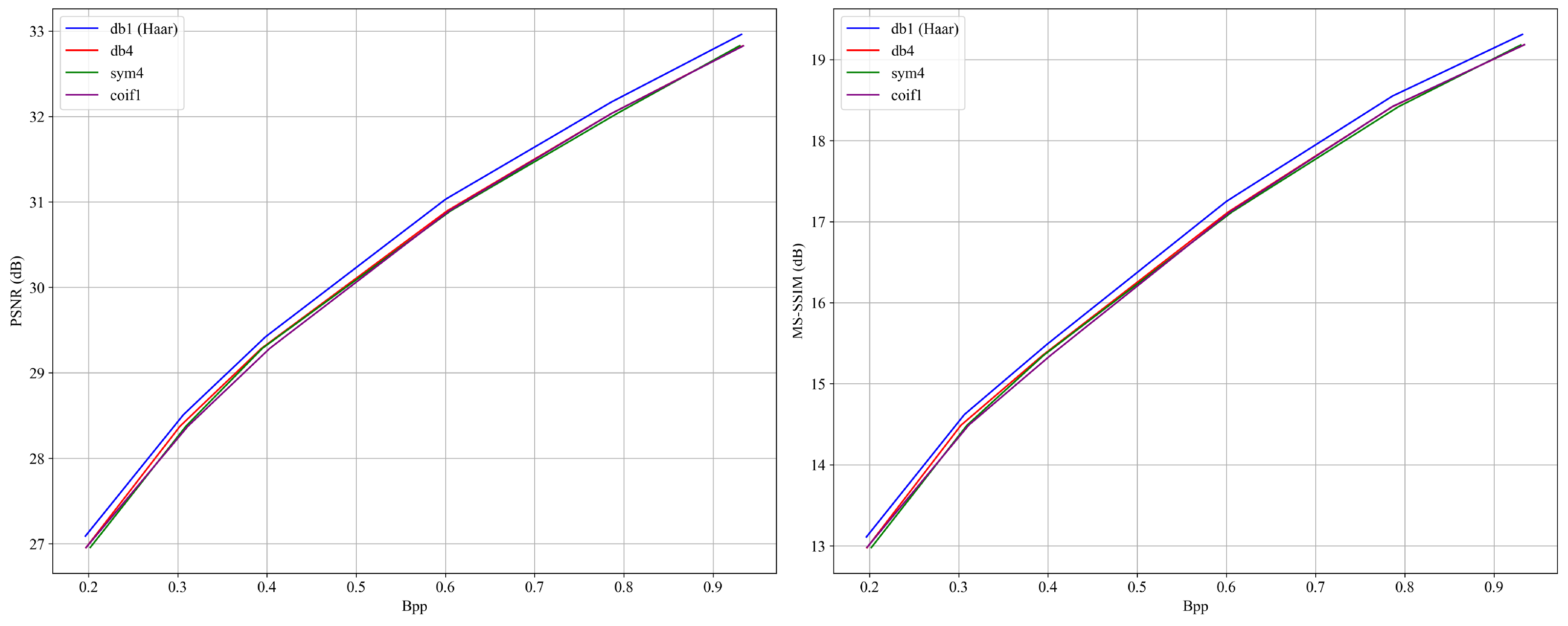
4.4.1. Impact of Wavelet Basis Selection

The wavelet basis determines how input features are decomposed into different frequency bands and directly affects the model’s ability to preserve structural details and compress redundant information. In this study, the Haar wavelet (db1) is adopted as the default wavelet basis due to its unique theoretical and empirical advantages.

As the shortest orthogonal wavelet (support length = 2), Haar offers high sensitivity to sharp transitions and structural boundaries, making it particularly effective in capturing edges of human-made objects such as roads and buildings [44,45,46]. Its strict orthogonality ensures lossless information representation during forward and inverse transforms, contributing to stable and accurate reconstruction. Moreover, Haar’s high computational efficiency—attributable to its simple filter structure—facilitates seamless integration into CNN-based architectures and reduces overall computation overhead.

From an empirical perspective, remote sensing images often involve diverse land-cover types and complex textures with high spatial variability across regions. The Haar wavelet effectively separates low-frequency structures (e.g., terrain contours) from high-frequency details (e.g., rooftops, vegetation boundaries), offering a favorable balance between structural fidelity and perceptual quality [47].

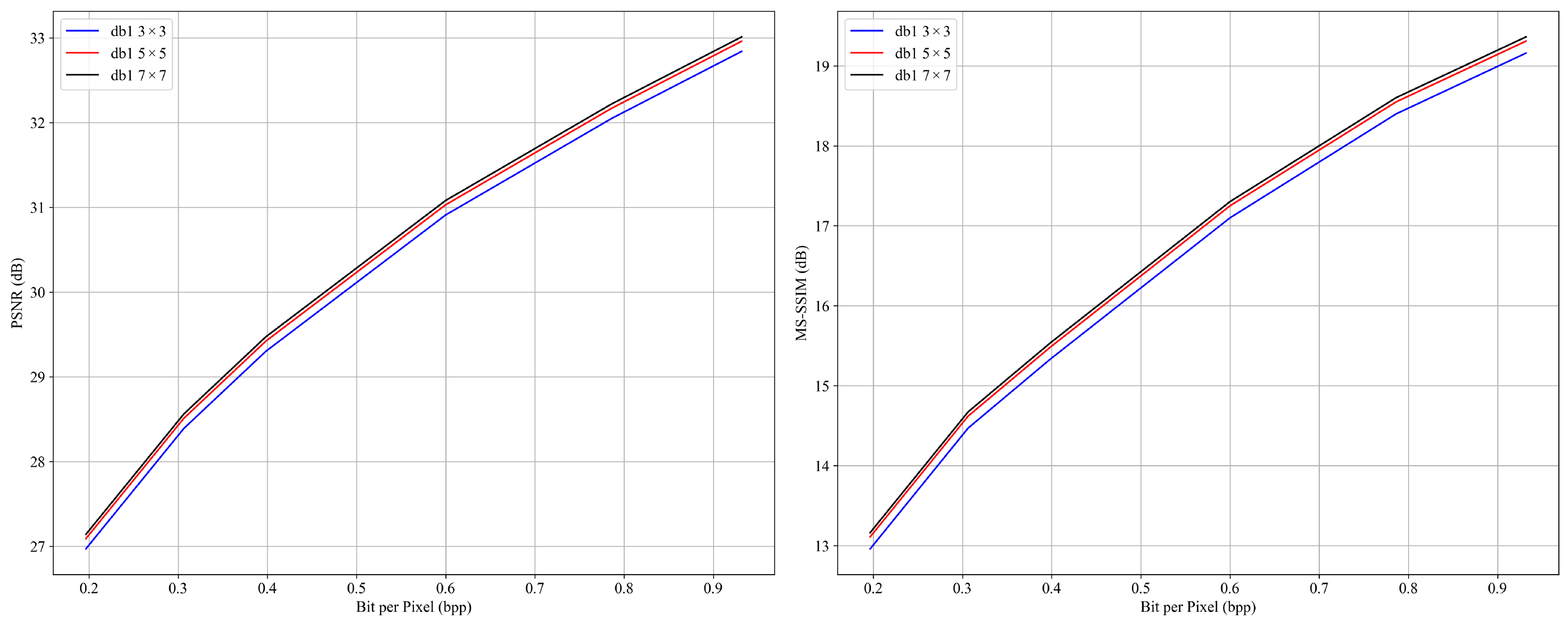
To further validate the suitability of the Haar wavelet, a comparative ablation study is conducted on the UC Merced dataset. Several representative wavelet bases are evaluated, including Daubechies-4 (db4), Symlets-4 (sym4), and Coiflets-1 (coif1), with all other architectural parameters held constant. As shown in Figure 12, the Haar wavelet consistently achieves competitive rate-distortion (RD) performance and demonstrates stronger robustness in preserving geometric features.

4.4.2. Role of Convolution Kernel Size and Performance–Efficiency Trade-Off

While wavelet basis selection influences frequency domain modeling, the convolution kernel size serves as the primary factor in controlling the model’s receptive field, which is crucial for capturing complex spatial dependencies in remote sensing images.

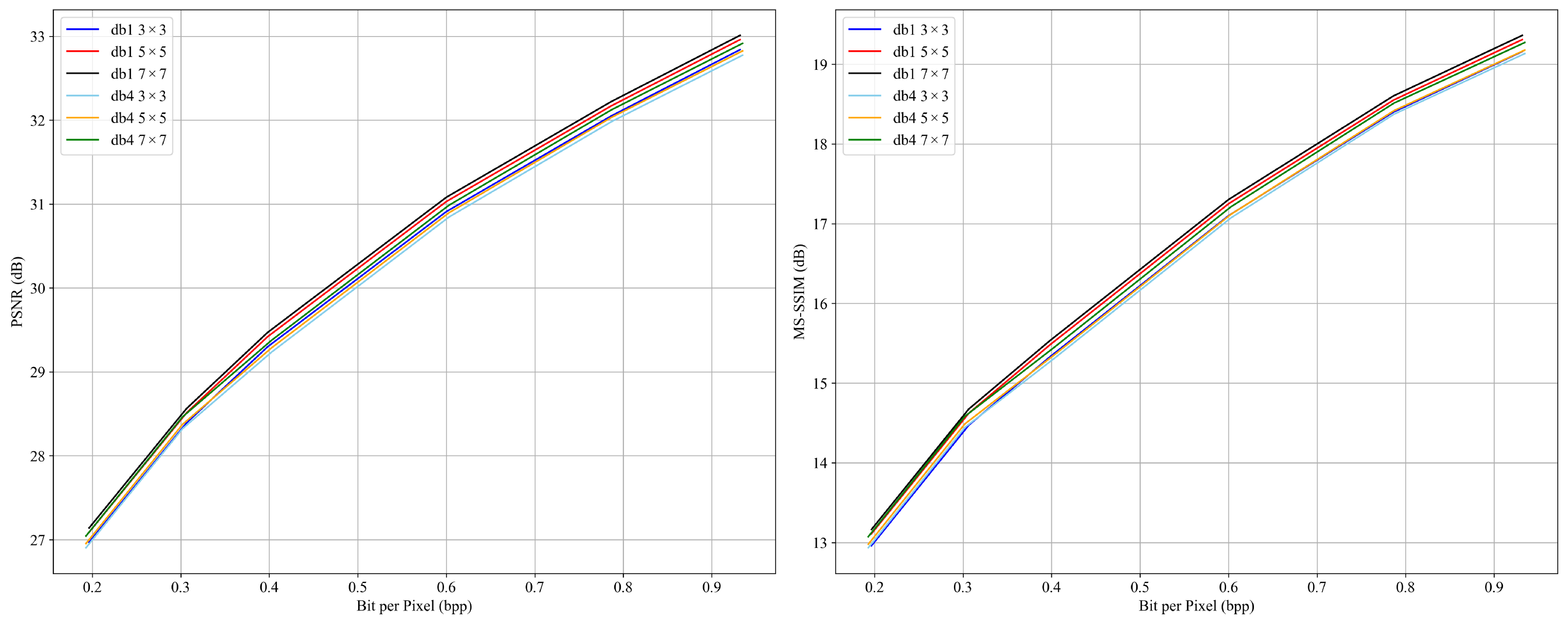
To investigate this, we perform controlled experiments using kernel sizes of 3 × 3, 5 × 5, and 7 × 7, under both Haar and Daubechies-4 configurations. The results are shown in Figure 13 and Figure 14.

The findings reveal that increasing the kernel size substantially expands the receptive field, enhancing the model’s ability to capture long-range spatial dependencies and cross-region structural correlations. This is particularly critical for remote sensing scenes involving non-local continuity, such as road networks, rivers, and mountain ranges.

Larger kernels also strengthen the synergy between convolutional modeling and wavelet-guided frequency decoupling, allowing for a clearer separation of low- and high-frequency features. This improves the model’s capacity to balance structure preservation and texture reconstruction, which directly translates to enhanced reconstruction quality.

However, as shown in

Table 1. Evaluation of the computational efficiency across different wavelet bases and kernel sizes.

Wavelet Basis	Kernel Size	Params (M)	FLOPs (G)	Enc-Time (s)	Dec-Time (s)
Haar	$5\times 5$	56.79	80.76	0.122	0.115
Haar	$3\times 3$	55.32	78.51	0.118	0.101
Haar	$7\times 7$	58.95	82.61	0.158	0.126

, increasing the kernel size results in a noticeable rise in parameter count, FLOPs, and inference time. For instance, switching from a 3 × 3 to a 7 × 7 kernel increases decoding time by over 20%. This trade-off becomes especially significant in real-world applications involving high-resolution data, limited hardware, or edge deployment scenarios.

4.4.3. Final Configuration and Design Considerations

In summary, the convolution kernel size in the WTLS module plays a dominant role in shaping the receptive field and enhancing spatial modeling capability, while the wavelet basis acts more as a tuning factor in frequency-domain decoupling.

Although both influence the model’s performance, kernel size exerts a more direct impact, especially in large-scale, structurally complex scenes.

Considering the trade-off between modeling accuracy, computational cost, and remote sensing adaptability, the Haar wavelet combined with a 5 × 5 convolution kernel is adopted as the default configuration for the WTLS module. This setup achieves a well-balanced solution in terms of structure fidelity, compression quality, and deployment efficiency.

4.5. Rate-Distortion Performance

In this study, we assess the rate-distortion characteristics of all models using four evaluation metrics: PSNR, MS-SSIM, LPIPS, and VIFp. Figure 15, Figure 16 and Figure 17 illustrate the rate-distortion curves for various compression approaches. Additionally, cross-dataset generalization is examined in Figure 18 and Figure 19.

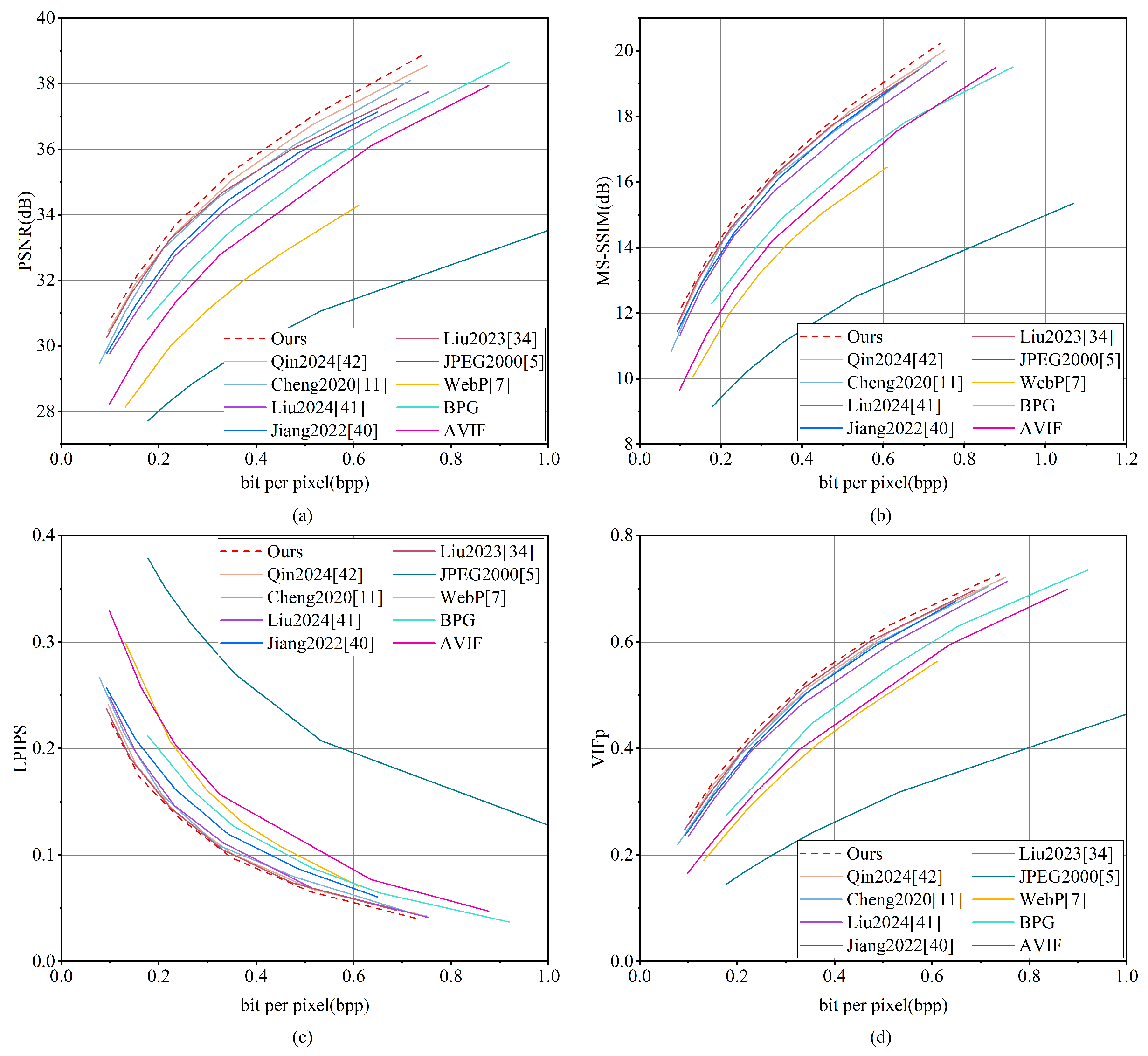
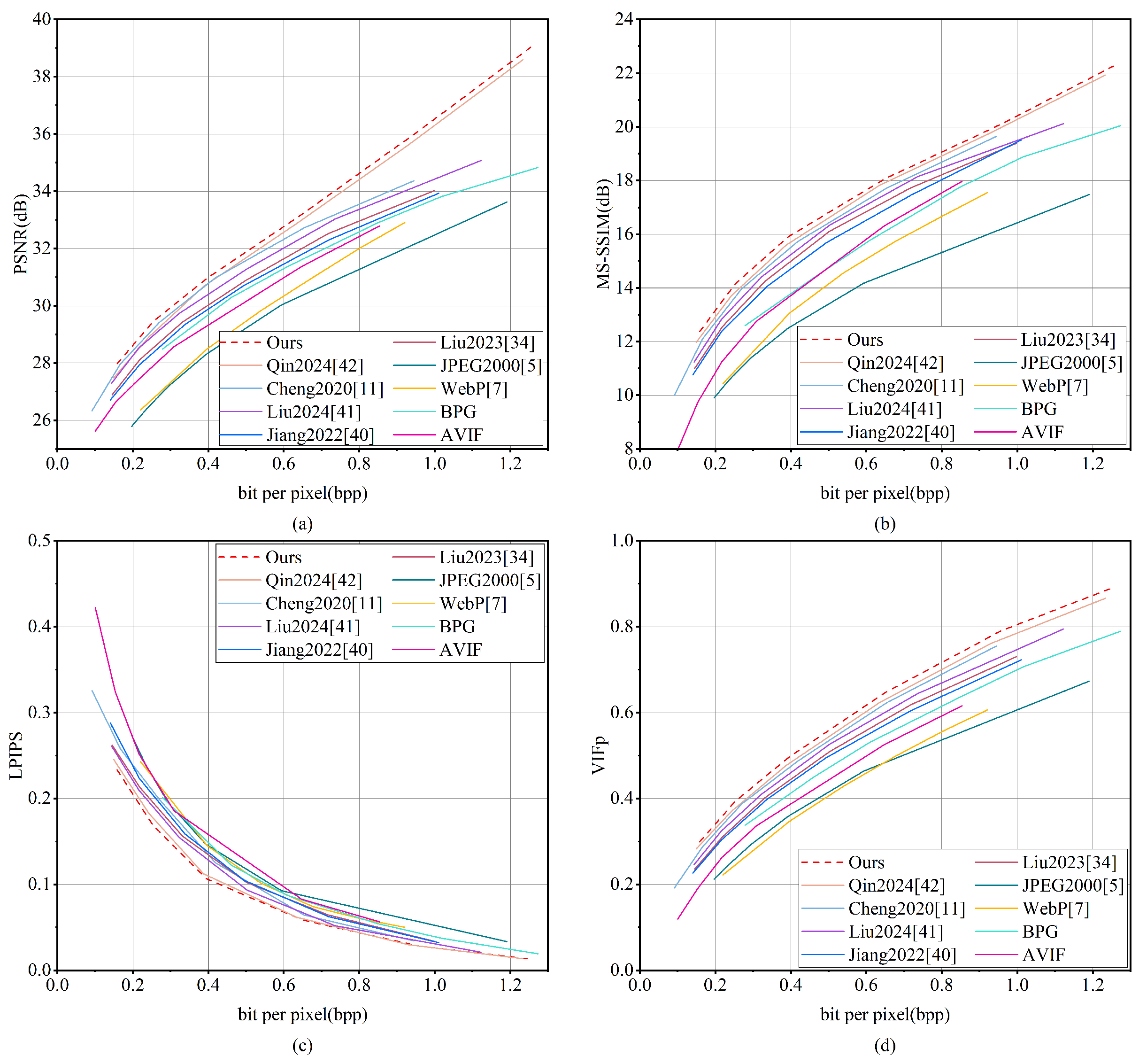
Figure 15 illustrates the rate-distortion curves for several compression techniques assessed using the DOTA dataset. It is noteworthy that MGMNet demonstrates superior performance compared to all other methods in terms of PSNR and MS-SSIM. This finding suggests that MGMNet exhibits enhanced rate-distortion efficiency while effectively maintaining both radiometric fidelity and structural integrity. Qin 2024 [42] ranks closely behind MGMNet in PSNR and MS-SSIM and shows comparable results to Liu 2024 [41] in LPIPS and VIFp. MGMNet also achieves the lowest LPIPS scores, suggesting better alignment with human perceptual quality, and attains the highest VIFp scores, reflecting superior retention of fine-grained details and high-frequency information.

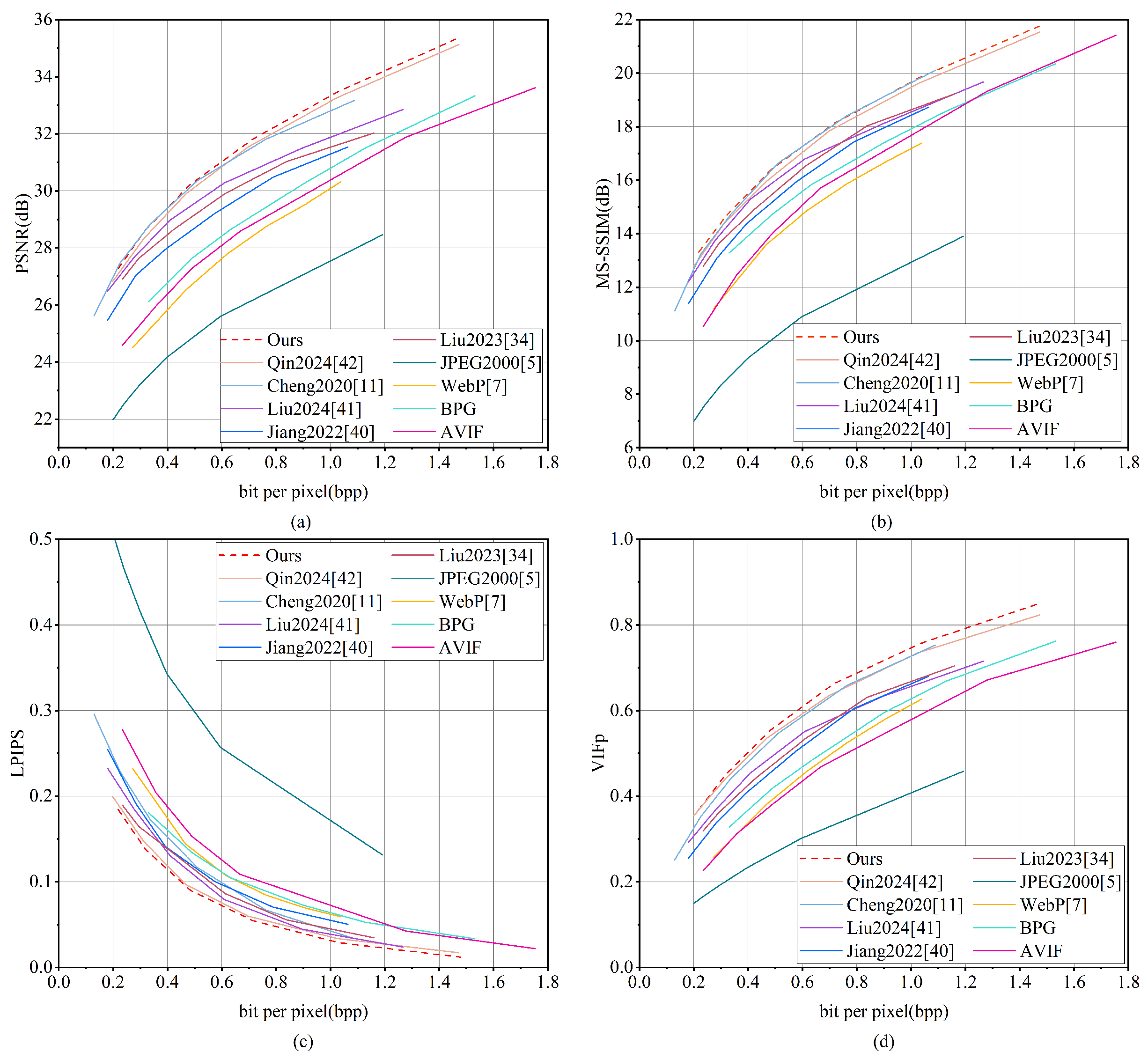
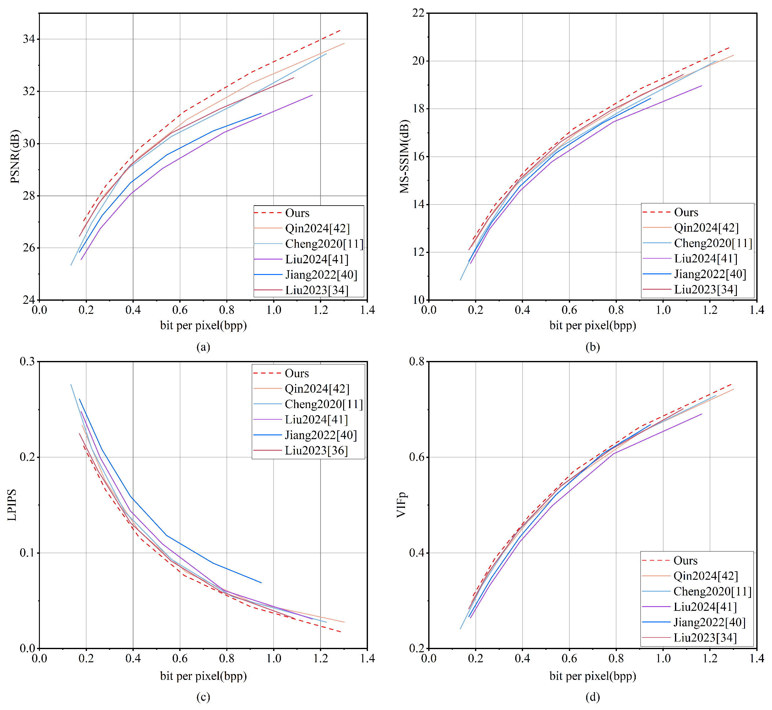
Figure 16 presents the rate-distortion curves for the UC-Merced dataset. MGMNet demonstrates performance in terms of PSNR that is comparable to Cheng 2020 [11] at lower bitrates, while exceeding it at higher bitrates. Furthermore, MGMNet consistently outperforms all other methodologies, with the exception of Cheng 2020 [11], across the entire range of bitrates. In terms of MS-SSIM, MGMNet closely aligns with Cheng 2020 [11] but significantly outperforms all other methods. Additionally, MGMNet exhibits the lowest distortion across bitrates for the LPIPS metric and shows superior performance on the VIFp metric.

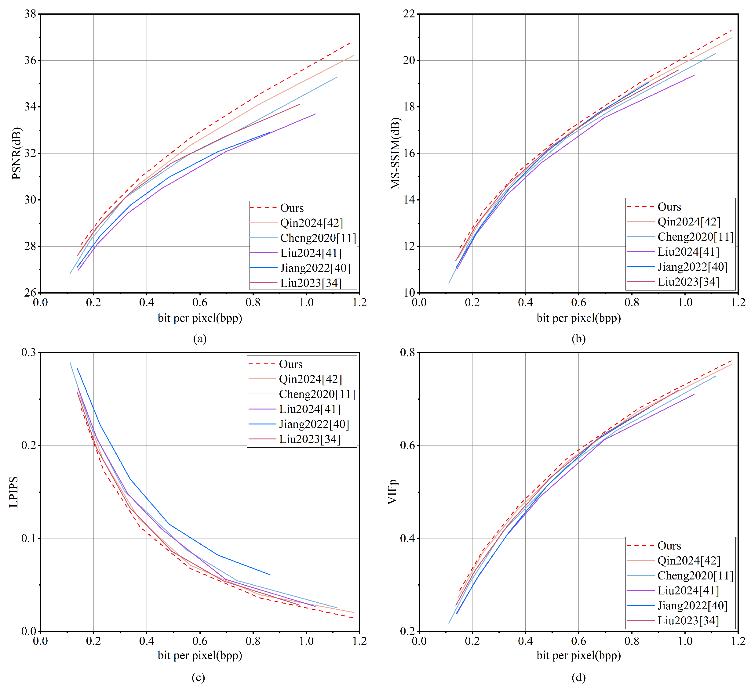
Figure 17 shows the results on NWPU-RESISC45, where MGMNet outperforms all comparison methods in PSNR, MS-SSIM, and VIFp, especially at high bitrates. In terms of LPIPS, MGMNet surpasses Qin 2024 [42] at low bitrates and performs comparably at high bitrates, while consistently outperforming the remaining methods.

To validate its robustness, we evaluated MGMNet on the validation sets of UC-Merced and NWPU-RESISC45 using a model trained on DOTA. As shown in Figure 18 and Figure 19, under cross-dataset validation, MGMNet demonstrates excellent performance in all four metrics. These results confirm MGMNet’s strong generalization capability and its effectiveness for remote sensing image compression.

We compute average BD-rate and BD-PSNR for MGMNet and other comparative methods relative to JPEG2000 as the baseline anchor, as shown in

Table 2. BD-rate and BD-PSNR comparisons of MGMNet and other methods, using JPEG2000 as the anchor reference.

Model	DOTA		UC-Merced		NWPU-RESISC45
	BD-Rate	BD-PSNR	BD-Rate	BD-PSNR	BD-Rate	BD-PSNR
WebP	−43.079%	2.000 dB	−40.364%	2.079 dB	−7.251%	0.389 dB
BPG	−63.976%	3.765 dB	−52.425%	2.873 dB	−25.557%	1.435 dB
AVIF	−58.221%	3.279 dB	−47.959%	2.524 dB	−19.765%	0.983 dB
Cheng2020 ([11])	−75.206%	5.116 dB	−70.973%	5.279 dB	−41.238%	2.281 dB
Jiang2022 ([40])	−71.633%	4.747 dB	−64.888%	3.789 dB	−29.224%	1.458 dB
Liu2023 ([34])	−75.217%	5.131 dB	−67.845%	4.195 dB	−31.684%	1.637 dB
Liu2024 ([41])	−69.802%	4.551 dB	−67.299%	4.563 dB	−37.246%	2.019 dB
Qin2024 ([42])	−77.171%	5.277 dB	−70.301%	5.275 dB	−42.143%	2.658 dB
Ours	−78.198%	5.519 dB	−72.021%	5.473 dB	−43.808%	2.866 dB

. BD-rate measures the difference in bit rate between different compression algorithms at the same image quality typically expressed as a percentage. In comparison, a negative value suggests a lower bit rate, indicating better compression efficiency. BD-PSNR reflects the change in image quality (measured by PSNR) at the same bit rate across different compression algorithms, usually expressed in dB. A positive value means the new method provides a higher PSNR at the same bit rate to yield better image quality. In comparison, a negative value indicates a lower PSNR and poorer quality. Table 2 shows that MGMNet achieves the most excellent BD-rate savings across all three datasets while also providing the highest BD-PSNR improvement. This demonstrates its ability to deliver superior image quality at lower bit rates.

(1)

In the context of the DOTA dataset, MGMNet demonstrates a significant reduction in the bit rate of 78.198% when compared to JPEG2000. When compared to other methods, MGMNet achieves a BD-rate reduction of 35.119%, 14.222%, 19.977%, 2.992%, 6.565%, 2.981%, 8.396%, and 1.027% compared to WebP, BPG, AVIF, Cheng 2020 [11], Jiang 2022 [40], Liu 2023 [34], Liu 2024 [41], and Qin 2024 [42], respectively. At the same bit rate, MGMNet also improves BD-PSNR by 3.519 dB, 1.754 dB, 2.240 dB, 0.403 dB, 0.772 dB, 0.388 dB, 0.968 dB, and 0.242 dB compared to these methods.

(2)

On the UC-Merced dataset, MGMNet reduces the bit rate by 72.021% when maintaining the same image quality as JPEG2000. Under identical bit rate conditions, it also delivers a 5.473 dB gain in PSNR. When compared to other methods, MGMNet reduces BD-rate by 31.657%, 19.596%, 24.062%, 1.048%, 7.133%, 4.176%, 4.722%, and 1.720% relative to WebP, BPG, AVIF, Cheng 2020 [11], Jiang 2022 [40], Liu 2023 [34], Liu 2024 [41], and Qin 2024 [42], respectively. Additionally, at the same bit rate, MGMNet improves BD-PSNR by 3.394 dB, 2.600 dB, 2.949 dB, 0.194 dB, 1.684 dB, 1.278 dB, 0.910 dB, and 0.198 dB compared to these methods.

(3)

For the NWPU-RESISC45 dataset, MGMNet reduces the bit rate by 43.808% compared to JPEG2000 at the same image quality. Compared to other methods, MGMNet achieves BD-rate reductions of 36.557%, 18.251%, 24.043%, 2.570%, 14.584%, 12.124%, 6.562%, and 1.665% relative to WebP, BPG, AVIF, Cheng 2020 [11], Jiang 2022 [40], Liu 2023 [34], Liu 2024 [41], and Qin 2024 [42], respectively. At the same bit rate, MGMNet also improves BD-PSNR by 2.477 dB, 1.431 dB, 1.883 dB, 0.585 dB, 1.408 dB, 1.229 dB, 0.847 dB, and 0.208 dB compared to these methods.

In summary, MGMNet demonstrates significant bitrate savings and image quality improvement on three datasets, fully demonstrating its excellent compression efficiency and robustness.

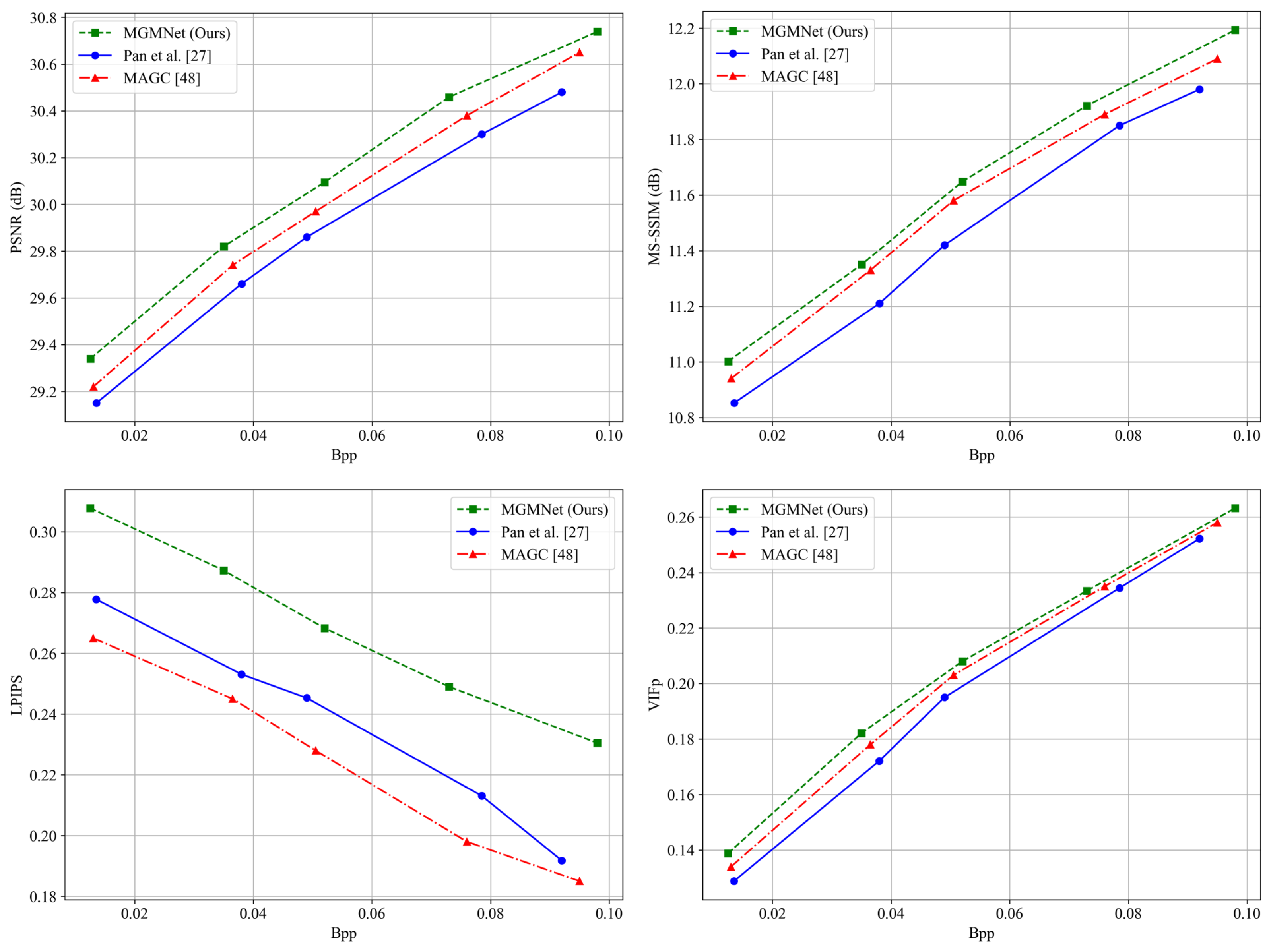
An additional performance evaluation is conducted on the DOTA dataset under extremely low bitrate conditions (BPP < 0.1). Two representative generative compression methods are introduced as baseline comparisons to assess the relative performance of the proposed approach.

(1)

Pan et al. [27] leverages a coupled generative network and compression module to enhance perceptual quality at ultra-low bitrates, particularly achieving favorable results on perceptual metrics such as LPIPS.

(2)

Ye et al. [48] introduces map-assisted semantic priors to guide content-aware reconstruction of remote sensing images, aiming to preserve land-cover structures even at extremely low bitrates.

The experimental results are shown in Figure 20. Although these generative approaches demonstrate advantages in perceptual quality, they typically rely on learned generative priors to hallucinate or fill in missing information caused by aggressive compression. Such generation-based mechanisms may introduce hallucinated details in high-texture regions of remote sensing imagery; for example, by producing non-existent road extensions, fabricated building outlines, or artificial textures.

In contrast, our proposed MGMNet does not rely on explicit generative priors. Instead, it explicitly models multi-scale spatial context and incorporates a wavelet-guided texture enhancement module to restore structural and textural details based on physically consistent and semantically faithful representations.

Under the BPP < 0.1 settings, MGMNet outperforms the above generative methods in objective metrics such as PSNR and MS-SSIM, demonstrating superior ability in recovering pixel-level accuracy and structural integrity.

On the LPIPS metric, MGMNet performs slightly below generative models. This is primarily because LPIPS measures similarity in deep feature space, favoring perceptual closeness rather than true fidelity to the original data source. Our approach places more emphasis on preserving spatial geometry and reconstructing authentic textures, avoiding the risk of introducing perceptually “plausible but incorrect” structures commonly found in generation-based reconstructions.

Overall, under ultra-low bitrate conditions, MGMNet achieves a better balance between structural fidelity and compression quality. The generated images are more geometrically consistent and semantically reliable, making the method well-suited for high-precision remote sensing applications where authenticity and accuracy are critical.

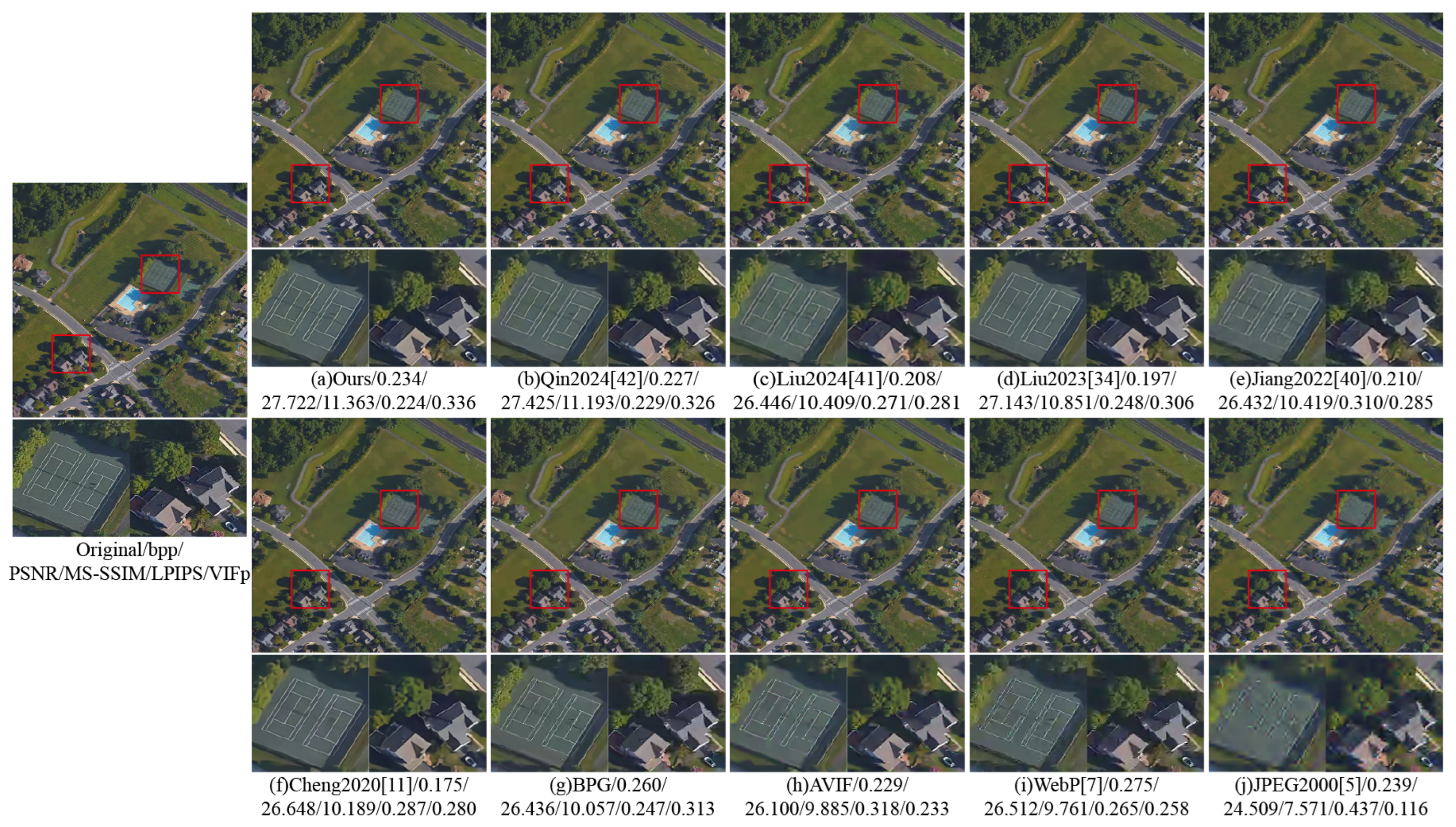
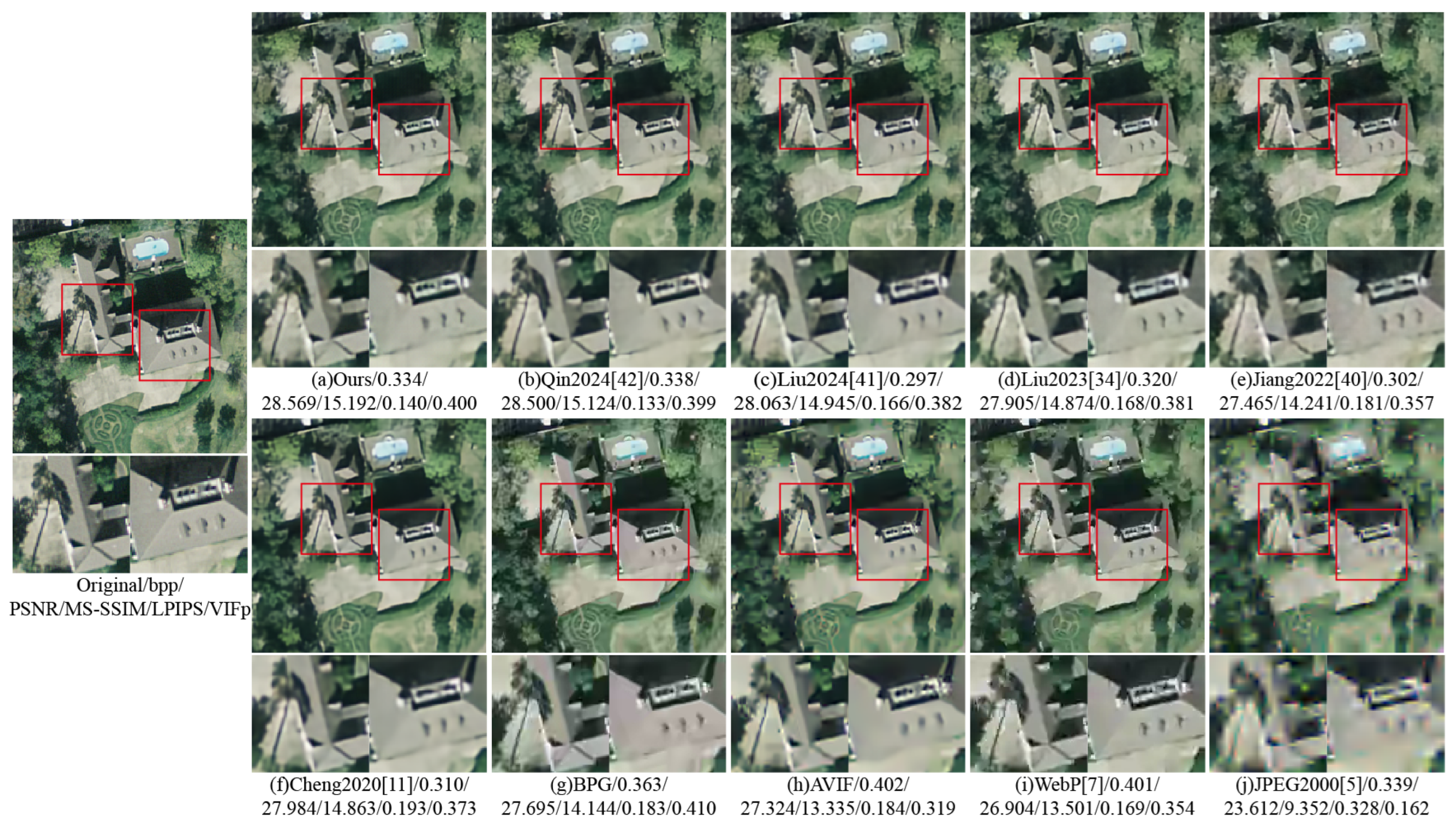
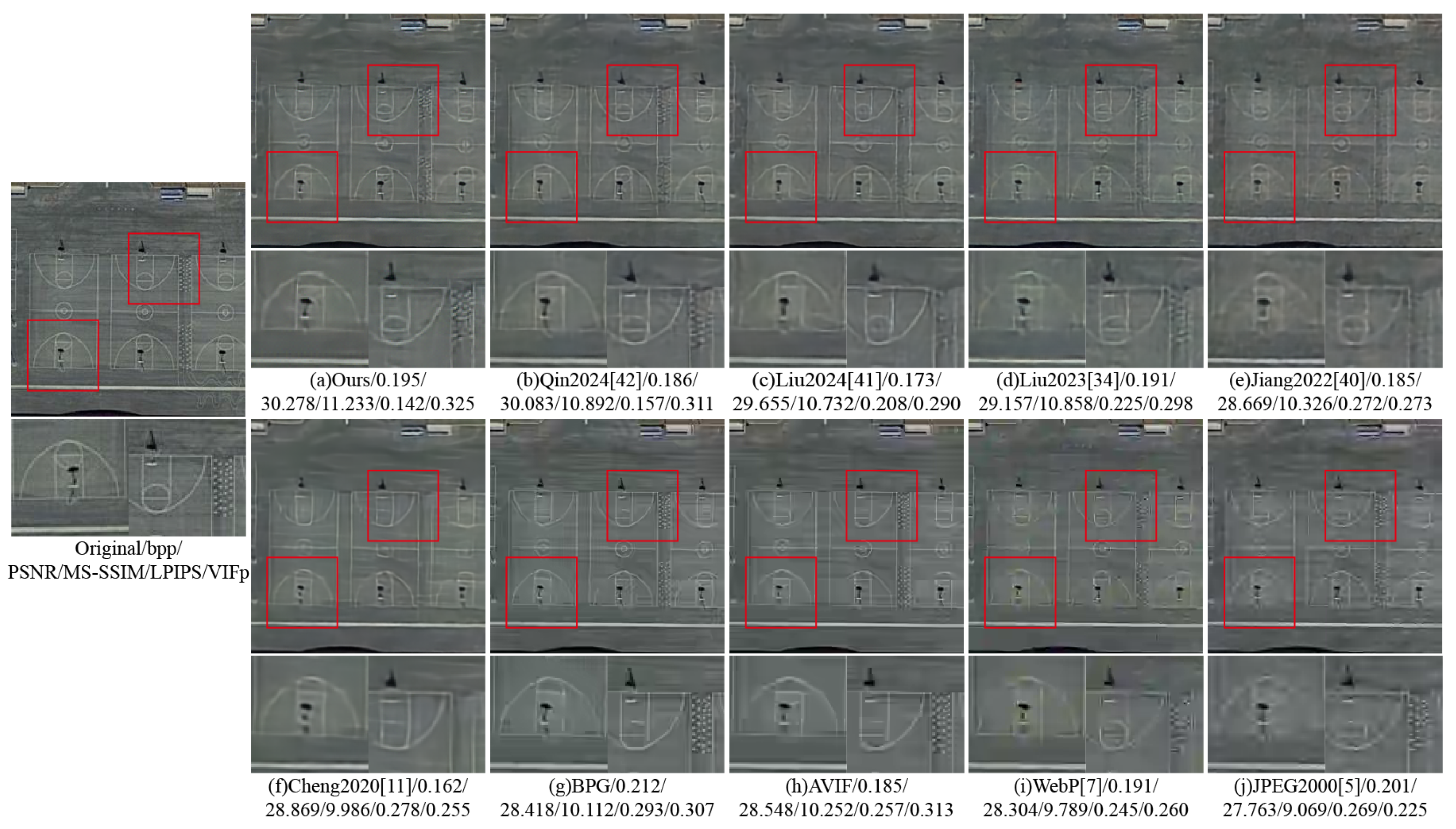
4.6. Visualization of Reconstructed Images

To verify the visual effect of MGMNet, this experiment visualizes and analyzes the reconstructed images from different methods. Figure 21, Figure 22 and Figure 23 show the reconstructed images and their zoomed-in regions for different datasets.

In Figure 21, among the four traditional compression methods, BPG produces visually superior results compared to AVIF, WebP, and JPEG2000. For example, the BPG-reconstructed image clearly shows the tennis court’s grid lines and the outlines of the buildings, while AVIF, WebP, and JPEG2000 exhibit noticeable distortions and blurring. Compared to MGMNet, although BPG achieves a slightly higher bitrate, MGMNet obtains a significant 1.286 dB gain in PSNR. MGMNet also delivers better visual quality, with clearer grid lines and sharper object boundaries.

Moreover, as demonstrated in Figure 22 and Figure 23, MGMNet consistently exhibits enhanced visual performance across the other two datasets. These findings further corroborate its robust generalization ability and resilience in various remote sensing contexts. In summary, MGMNet not only excels in preserving visual details but also in compression efficiency, highlighting its efficacy and potential applicability in remote sensing image compression endeavors.

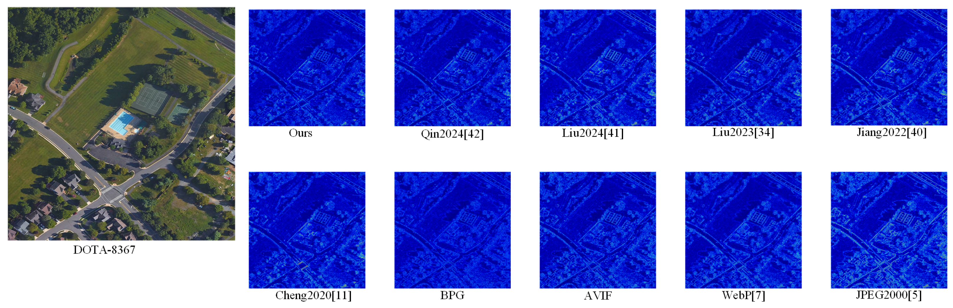
To complement the quantitative metrics in Table 2—where performance differences across methods remain relatively small—pixel-level error heatmaps are employed for qualitative comparison. A detailed pixel-level difference analysis is performed based on the reconstructed results shown in Figure 21, and the corresponding error heatmaps are presented in Figure 24. These heatmaps visualize the absolute per-pixel reconstruction error between the original and compressed images, offering clearer insight into performance differences in structurally critical areas.

The error values are computed as absolute differences at the pixel level and visualized using the Jet colormap, producing heatmaps where cool colors (e.g., blue) represent low error and warm colors (e.g., red) indicate high error. To enhance the visibility of fine residuals in low-error regions, a contrast enhancement factor is applied during heatmap generation, making subtle differences more discernible—particularly in high-resolution remote sensing images that contain rich structural textures.

As illustrated in Figure 24, the proposed method yields uniformly low error across the image. Most regions appear in cool tones, demonstrating strong performance in both texture recovery and structure preservation. Compared to other approaches, fewer high-error regions are observed, especially in edge areas and fine textures, highlighting the method’s superiority in spatial fidelity and detail reconstruction.

Compared to existing deep learning-based approaches, MGMNet demonstrates enhanced capability in restoring fine-grained image details at similar bits per pixel (bpp) levels. It also achieves higher performance in terms of both PSNR and MS-SSIM metrics. In the red-marked regions, Jiang 2022 [40] and Liu 2024 [41] fail to fully reconstruct the gridlines and exhibit artifacts and noise. Liu 2023 [34] and Cheng 2020 [11] exhibit an over-smoothing effect on the vegetation situated behind the residence, which consequently leads to a diminution of high-frequency information. In contrast, MGMNet preserves more texture and sharper edges. Compared with Qin 2024 [42], MGMNet also reconstructs richer textures and more defined contours.

4.7. Ablation Experiments

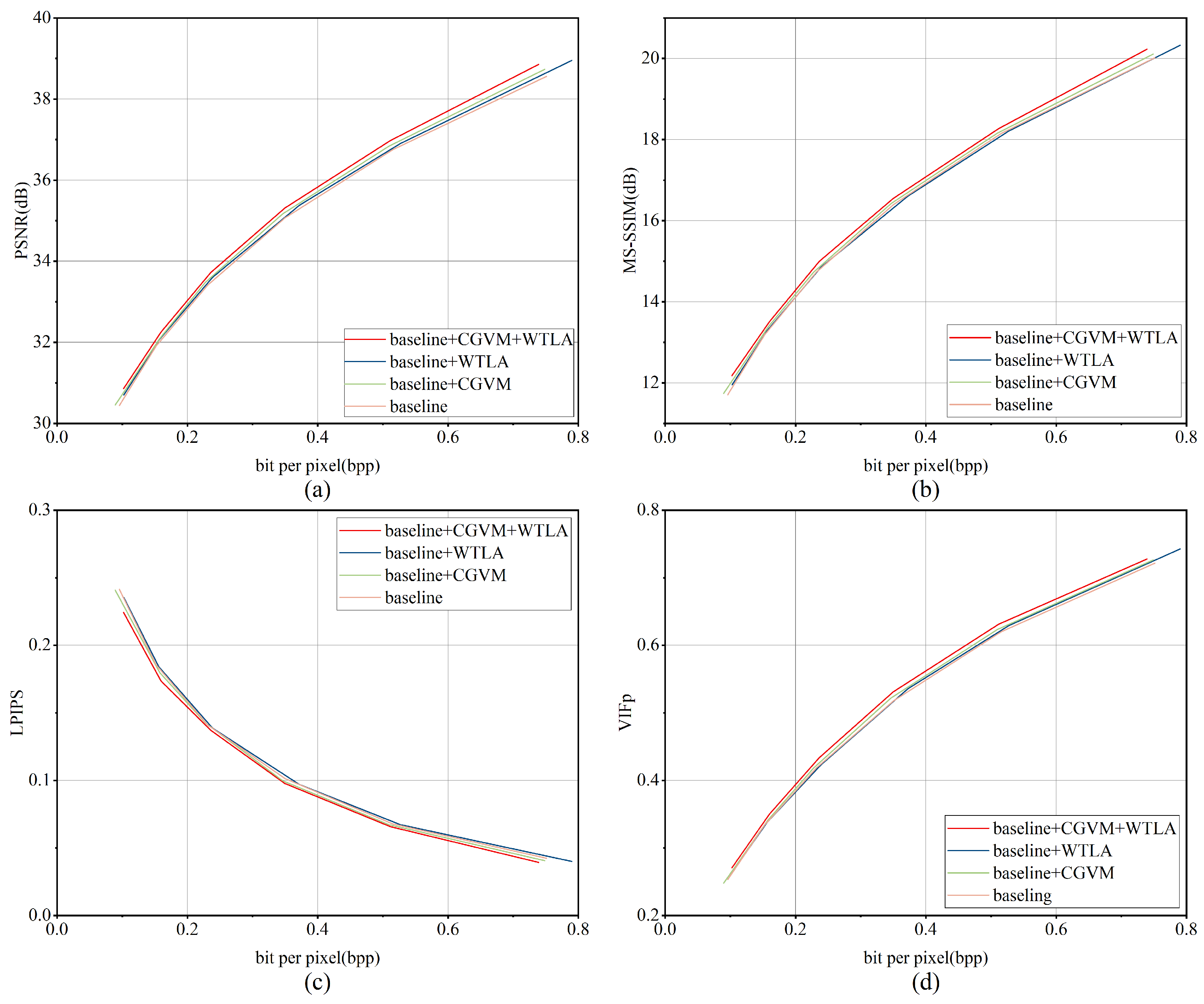
To evaluate the impact of each module, we conducted ablation experiments utilizing the DOTA dataset. The findings are illustrated in Figure 25. Here, the baseline refers to the original network Qin 2024 [42]. Baseline + CGIM denotes the baseline integrated with the Channel–Global Information Module (CGIM). Baseline + WTLS represents the baseline combined with the Wavelet-Transform Local Structure module (WTLS). Baseline + CGIM + WTLS includes both modules integrated simultaneously.

As shown in Figure 25, adding CGIM to the baseline significantly improves rate-distortion performance at similar bitrates. This demonstrates the importance of incorporating channel-wise and global contextual information for accurate remote-sensing image reconstruction.

The baseline + WTLS configuration shows a clear PSNR improvement over the baseline. However, the gains in MS-SSIM and LPIPS are relatively limited. In terms of VIFp, baseline + WTLS performs on par with the baseline at low bitrates and surpasses it at higher bitrates. These results highlight WTLS’s effectiveness in capturing multi-scale local features and enhancing structural quality.

The integrated model, which includes the baseline, CGIM, and WTLS components, consistently exhibits enhanced performance across all assessed metrics. This suggests that the combined integration of CGIM and WTLS facilitates a more thorough representation of features. The proposed architecture enables the model to proficiently learn and assimilate local, channel, and global features, ensuring the preservation of essential information and promoting accurate, high-fidelity image reconstruction.

To further demonstrate the effectiveness of each component, we compute the average BD-rate and BD-PSNR for baseline + CGIM, baseline + WTLS, and baseline + CGIM + WTLS, using the baseline as the reference point. The results are presented in

Table 3. Results of ablation experiments on the DOTA dataset.

Model	BD-Rate	BD-PSNR
baseline + CGIM	−3.262%	0.154 dB
baseline + WTLS	−1.435%	0.067 dB
baseline + CGIM + WTLS	−5.918%	0.289 dB

.

(1)

For the same quality, baseline + CGIM achieves a 3.262% reduction in bit rate compared to the baseline, baseline + WTLS reduces the bit rate by 1.435%, and baseline + CGIM + WTLS leads to a 5.918% decrease.

(2)

For the same bit rate, baseline + CGIM shows a 0.154 dB increase in PSNR over baseline, baseline + WTLS achieves a 0.067 dB improvement, and baseline + CGIM + WTLS results in a 0.289 dB increase in PSNR.

The above results show that both CGIM and WTLS significantly improve image compression performance, while the combination of the two further enhances it.

4.8. Complexity Analysis

To ensure a fair assessment of computational complexity and resource consumption, all compression methods were evaluated on the DOTA validation set using identical hardware and environmental settings. The comparison considers FLOPs, parameter count, and average encoding/decoding times.

All evaluations were conducted with input images of size 3 × 256 × 256, and timing results represent averages to mitigate variations caused by GPU memory usage. The findings indicate that MGMNet attains an advantageous equilibrium between compression efficacy and computational efficiency. Two Transformer-based image compression [22,49] algorithms were further incorporated for comparative analysis, highlighting the computational efficiency of the proposed architecture.

As shown in

Table 4. Evaluation of the computational efficiency across different image compression techniques.

Method	FLOPs (G)	Params (M)	Encoding Time (s)	Decoding Time (s)
Cheng2020 [11]	27.41	8.78	0.118	0.097
Jiang2022 [40]	82.36	116.48	0.125	0.156
Zou2022 [22]	48.70	75.00	0.283	0.272
Entroformer [49]	44.65	78.32	0.185	0.152
Liu2023 [34]	116.78	75.90	0.139	0.145
Liu2024 [41]	190.55	91.17	0.110	0.121
Qin2024 [42]	65.56	47.88	0.098	0.114
Ours	80.76	56.79	0.122	0.115

, in terms of FLOPs, MGMNet incurs an increase of 53.35 G and 15.20 G compared to Cheng 2020 [11] and Qin 2024 [42], respectively. However, it achieves reductions of 1.94%, 30.84%, and 57.61% compared to Jiang 2022 [40], Liu 2023 [34], and Liu 2024 [41], respectively. Regarding model parameters, MGMNet reduces the parameter count by 51.24%, 25.18%, and 37.71% compared to Jiang 2022 [40], Liu 2023 [34], and Liu 2024 [41], respectively, while exhibiting an increase of 48.01 M and 8.91 M compared to Cheng 2020 [11] and Qin 2024 [42].

4.9. Task-Oriented Performance

To assess the practical effectiveness of the proposed compression method in downstream remote sensing tasks, salient object detection is selected as a representative evaluation scenario [50]. This task provides a high-level vision benchmark that is sensitive to both structural integrity and semantic preservation, making it suitable for evaluating compressed image quality.

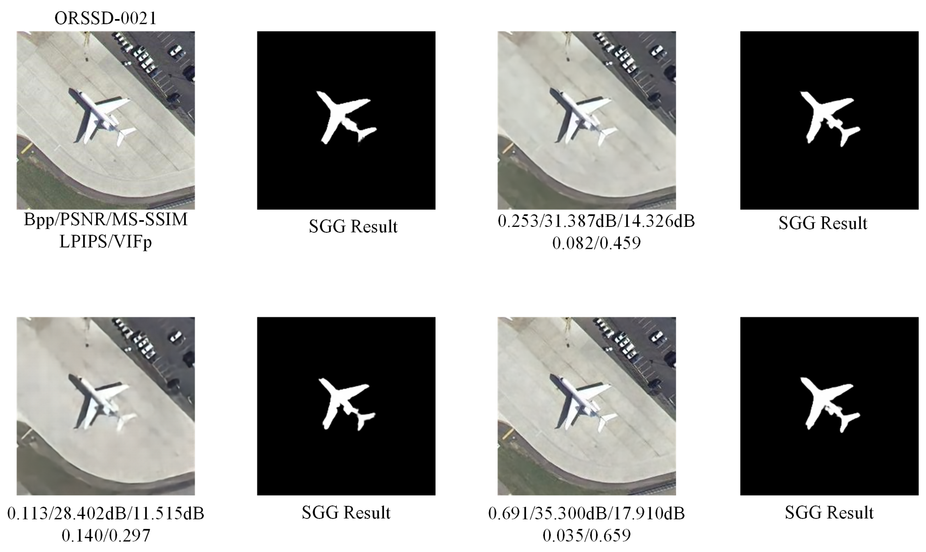
The widely used SggNet model [50] is adopted for saliency prediction, with the ORSSD dataset [51] serving as the evaluation benchmark. ORSSD contains a diverse range of land-cover categories, including urban and natural scenes, and is designed for tasks involving fine-grained structural understanding. To ensure reproducibility and demonstrate representative performance, a sample image (ID: 0021) is randomly selected from the ORSSD test set for qualitative and quantitative analysis.

During the experiment, the trained compression model is applied to compress and reconstruct the test images under varying bitrate settings, measured in bits per pixel (BPP). Each reconstructed image is then fed into the SggNet to perform salient object detection. To evaluate how well the compressed images preserve task-relevant information, we adopt three commonly used metrics: F-measure [52], S-measure [53], and Mean Absolute Error (MAE) [54]. These metrics, respectively, measure the precision-recall balance, structural similarity, and pixel-level accuracy between the predicted saliency maps and the ground truth.

The results, summarized in

Table 5. Evaluation results of ORSSD-0021 under different bitrate settings using three metrics.

Image	S-Measure	F-Measure	MAE
Original	0.9452	0.9051	0.006549
Bpp = 0.113	0.9288	0.8777	0.007654
Bpp = 0.253	0.9360	0.8920	0.007432
Bpp = 0.691	0.9394	0.8971	0.007128

, demonstrate that the proposed method maintains high detection performance across all compression levels. Even under low-bitrate conditions (e.g., BPP = 0.113), the reconstructed images retain sufficient structure and semantics to support accurate saliency detection, as reflected by only slight degradation in all three evaluation metrics.

In addition to the quantitative analysis, Figure 26 provides a visual comparison of the detection results on ORSSD-0021. The original and compressed reconstructed images are processed by SggNet, and the resulting saliency maps are shown side by side for comparison.

5. Conclusions

This research presents MGMNet, a lightweight compression framework specifically designed for remote sensing imagery. It leverages the sequence modeling capabilities inherent in state–space networks, combined with channel-aware semantic enhancement, to enhance compression efficacy. In light of the escalating complexity and volume of remote sensing data, MGMNet confronts significant compression challenges by incorporating two innovative modules: the Wavelet Transform-guided Local Structure Decoupling (WTLS) module and the Channel–Global Information Modeling (CGIM) module. The WTLS module employs a multi-scale decomposition approach to separate structural contours from fine-grained textures, facilitating the parallel modeling of various frequency bands while preserving a streamlined architecture. Concurrently, the CGIM module bolsters global modeling proficiency through directionally selective state–space scanning and dynamic spatial–channel reweighting, thereby effectively capturing both semantic relevance and local discriminability.

Future research will aim to adapt the proposed framework to hyperspectral and multi-temporal remote sensing data. These scenarios involve complex spectral dependencies and temporal variations, posing greater challenges for compression.