Improving the Estimates of County-Level Forest Attributes Using GEDI and Landsat-Derived Auxiliary Information in Fay–Herriot Models

Abstract

National-scale forest inventories such as the Forest Inventory and Analysis (FIA) program in the United States are designed to provide data and estimates that meet target precision at the national and state levels. However, such design-based direct estimates are often not accurate at a smaller geographic scale due to the small sample size. Small area estimation (SAE) techniques provide precise estimates at small domains by borrowing strength from remotely sensed auxiliary information. This study combined the FIA direct estimates with gridded mean canopy heights derived from recently published Global Ecosystem Dynamics Investigation (GEDI) Level 3 data and Landsat data to improve county-level estimates of total and merchantable volume, aboveground biomass, and basal area in the states of Alabama and Mississippi, USA. Compared with the FIA direct estimates, the area-level SAE models reduced root mean square error for all variables of interest. The multi-state SAE models had a mean relative standard error of 0.67. In contrast, single-state models had relative standard errors of 0.54 and 0.59 for Alabama and Mississippi, respectively. Despite GEDI’s limited footprints, this study reveals its potential to reduce direct estimate errors at the sub-state level when combined with Landsat bands through the small area estimation technique.

1. Introduction

National forest inventories (NFIs) are usually designed to provide data and estimates that meet national and state-level target precision [1]. However, these data are used to make management and policy decisions at smaller geographical scales, such as at the sub-state and county levels [2,3]. The NFI data are processed to derive information on the status, trends, and condition of forests nationwide [1] and are critical in the assessment of the impact of climate change, wildfire, and invasive species on biodiversity as well as growth and yield modeling [4]. An example of NFI in the United States is the Forest Inventory and Analysis (FIA) program of the United States Department of Agriculture (USDA) Forest Service. In recent years, there has been a growing focus on enhancing the precision of estimates of forest attributes, e.g., volume, basal area, and biomass at smaller geographical scales [5,6,7,8,9,10,11,12,13,14].

The FIA uses a national-scale sampling approach and involves the measurement of different vegetation attributes in permanent plots on forested lands across the United States. Annually, 10–20 percent of these plots are measured for more than 27 tree-level attributes [15]. More than 100 other variables are then derived from these measured variables, and all measured and derived variables are made publicly available on the FIA Datamart (https://apps.fs.usda.gov/fia/datamart/datamart.html, accessed on 8 July 2024). Generally, good design-based sampling enables accurate and unbiased estimation of forest inventory attributes at the national scale. However, the direct estimates at smaller geographical scales, such as at the county level, are not always as accurate [1,16]. Due to this challenge, there has been a significant development in the use of the model-based approach, such as small area estimation (SAE), to improve the precision of NFI data at smaller domains without increasing sampling effort and cost [12,17,18].

SAE is a statistical technique that allows for the precise estimation of forest attributes utilizing ancillary data for areas with smaller samples [19]. The SAE technique is particularly suited in situations where there are insufficient ground samples to achieve estimates at a desired level of precision [5]. The “small” in the SAE refers to a domain for which reliable statistics of interest cannot be derived by using only the available data [20]. The SAE methods can be classified into three categories—direct, indirect, and composite estimators [5,8,21]. Typically, the direct estimators are derived by using only the data from the small area under study, while the indirect estimators are derived by linking the direct estimates with auxiliary information from within or outside the small domain through regression or imputation [21,22]. To balance the high variance of the direct estimators and the biasedness of the indirect estimator, a model that weighs the two estimators is used to produce a composite estimator. The composite estimator, which could be area-level [23] or unit-level [24], is based on a mixed-effect model and uses a weighted average to account for the model variation and the variation within the direct estimates of the small domains [8,19,23]. Area-level SAE has been widely applied to forest inventory, mainly because auxiliary data may not be available at the plot (unit) level or may not align properly in the case of FIA data due to the swapping and fuzziness of the plot locations. Additionally, the correlation between the direct estimates and the auxiliary information may be reduced due to the low precision of the global positioning system of plot locations [7].

In area-level SAE, the primary source of auxiliary information has been remotely sensed data obtained from various platforms and sensors. This is because remote sensing technologies can be used to retrieve reflectance information related to land cover, vegetation structure, and growth [25]. Also, the temporal and spatial coverage of remotely sensed data makes it relevant to vegetation and environmental studies at different scales. Satellite-based and aerial-level data, such as Landsat, aerial images, and lidar, have been used as auxiliary information with NFI data to improve the precision level of forest inventory attributes using SAE and related methods [6,7,17,22,26,27,28]. While aerial-level data provides high-resolution forest data, they can be expensive and limited, temporally. Thus, studies have mostly relied on publicly available satellite-based data for small area estimation. One of the publicly available satellite data sources is the Global Ecosystem Dynamics Investigation (GEDI).

GEDI is a spaceborne, high-resolution lidar that produces observations of the three-dimensional structure of the Earth. GEDI has been used to develop forest structure and compositional data such as canopy height metrics, aboveground biomass and carbon, and volume. However, no studies have reported the accuracy and precision level that can be achieved by combining GEDI (Level 3) and Landsat data as auxiliary information in an area-level SAE model, especially in the southeastern part of the United States.

Thus, the overall objective of this research was to determine the county-level precision achievable through the combination of GEDI Level 3 canopy height metrics and Landsat bands as auxiliary information with FIA data using the area-level SAE model in estimating forest attributes for the states of Alabama and Mississippi, USA. The specific objectives were to (1) examine the precision gain by the area-level composite estimators in estimating selected forest inventory attributes at single and multi-state levels, and (2) compare the performance of the direct and composite estimators regarding forest inventory attributes of individual counties. The variables of interest were merchantable cubic volume per hectare (CVM, m³ ha⁻¹) defined as the net merchantable bole volume of live trees with at least 12.7 cm (5 inches) diameter at breast height (dbh; diameter at 1.3 m (4.5 feet) above ground); total cubic volume per hectare (CVT, m³ ha⁻¹) defined as the gross volume of live trees with at least 12.7 cm (5 inches) dbh; aboveground biomass per hectare (AGB, Mg ha⁻¹), defined as the aboveground biomass of live trees with at least 2.54 cm (1 inch) dbh; and basal area per hectare (BA, m² ha⁻¹) defined as the cross-sectional area of live trees with at least 2.54 cm (1 inch) dbh. To our knowledge, our study is the first to assess the relevance of combining Landsat and canopy height metrics from spaceborne lidar–GEDI for small area estimation at the county level.

2. Materials and Methods

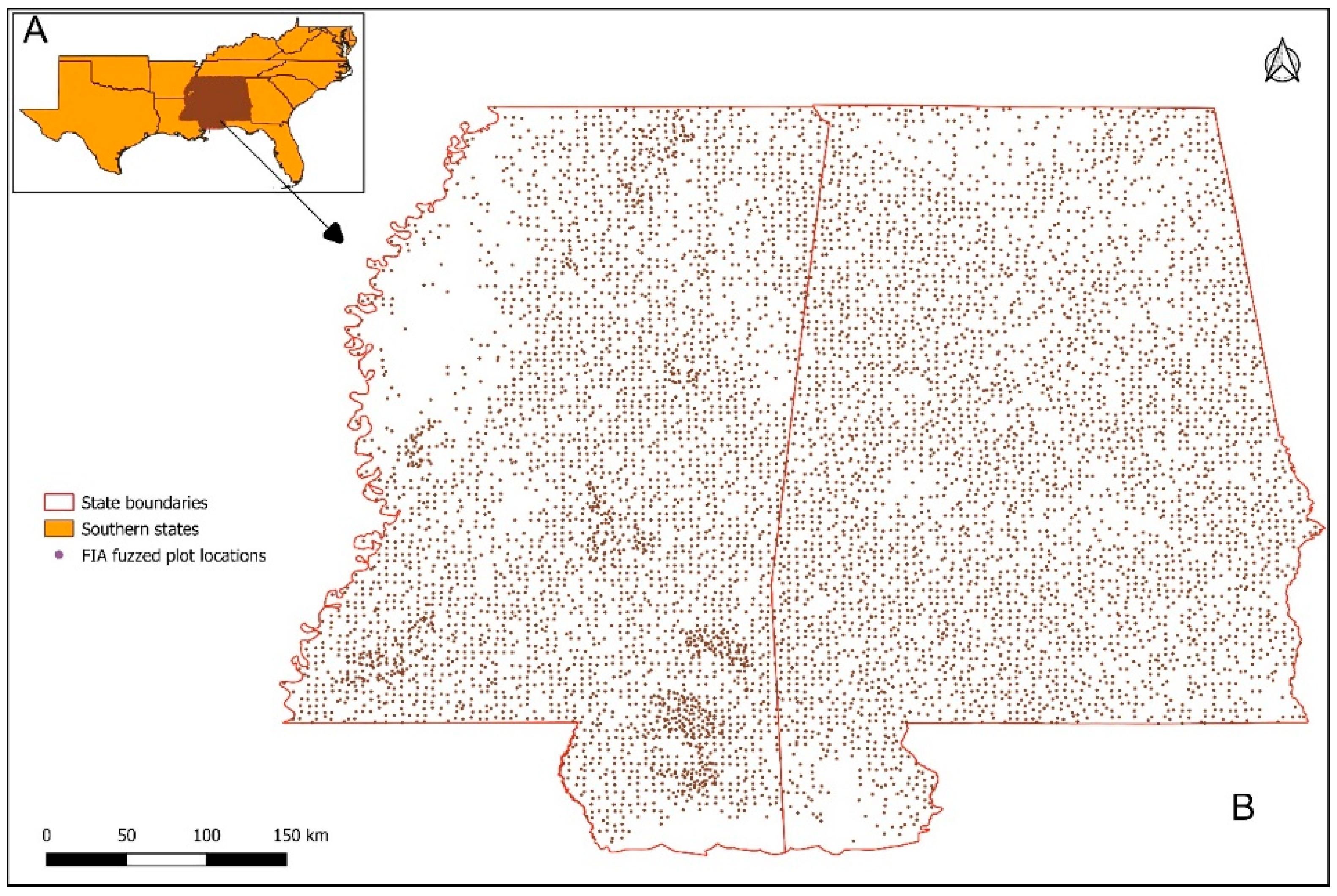
2.1. Study Area

The study area for this research included the states of Alabama and Mississippi, USA (Figure 1). Alabama has 67 counties and covers an area of 13.5 million ha (33.6 million acres). The state has four main soils, including dark loams and red clays, rich limestone, marl soils, varied soil within the mineral belt, sandy loams, and deep porous sands [29]. The average annual temperature is about 18 °C (64 °F), and it occasionally rises to 38 °C (100 °F), with an average elevation of about 150 m above sea level. More than two-thirds of the state is covered by forests of both hardwood and softwood species [30]. These species include loblolly pine (Pinus taeda, L.); shortleaf pine (Pinus echinata Mill.); white oak (Quercus alba L.); hickory species (Carya spp.); red maple (Acer rubrum, L.); sweetgum (Liquidambar styraciflua, L.); and yellow poplar (Liriodendron tulipifera, L.). Mississippi is a neighboring state to Alabama, with 82 counties covering an area of about 12.6 million ha (31 million acres) with various soil types. However, Natchez silt loam is the state’s primary soil type. The elevation ranges from 0 m to 246 m with an average elevation of 91.4 m. The mean annual temperature of the state ranges from 16.6 °C (62 °F) in the north to 20 °C (68 °F) along the coast. The state has both conifers (softwood) and broadleaf species (hardwood) such as loblolly pine (Pinus taeda, L.), the most frequently planted tree species; longleaf pine (Pinus palustris L.); eastern red cedar (Juniperus virginiana, L.); bald cypress (Taxodium distichum, (L.) Rich); and slash pine (Pinus elliottii, Engelm) [15].

2.2. Field Data

The field data used in this study were downloaded from the FIA Database (https://apps.fs.usda.gov/fia/datamart/datamart.html, accessed on 11 September 2023). The datasets consist of annual inventory data collected for both states throughout the full inventory cycle. Each year, the FIA measures up to 20% of the total FIA plots in a state, and the full cycle constitutes measurement of all the FIA plots within the state. In this study, we considered four variables of interest, namely CVM: merchantable volume (m³ ha⁻¹); CVT: total volume (m³ ha⁻¹); AGB: aboveground biomass (Mg ha⁻¹); and BA: basal area (m² ha⁻¹) and the method of measurement and derivation of these forest parameters follows a nationally consistent framework. Therefore, readers are referred to the comprehensive guidelines followed for measuring and estimating the parameters (https://usfs-public.app.box.com/v/FIA-NFI-FieldGuides/file/1694089849801; https://www.srs.fs.usda.gov/pubs/gtr/gtr_srs080/gtr_srs080.pdf, accessed on 11 June 2025). The county-level estimates of variables of interest were obtained using the FIA web application EVALIDator 2.1.0 (https://apps.fs.usda.gov/fiadb-api/evalidator; accessed on 11 September 2023) [31]. Estimates were based on plot measurements taken between 2015 and 2022 for Alabama and between 2016 and 2021 for Mississippi. An FIA plot is a cluster of four subplots. Each subplot consists of one 7.3 m (24 ft) radius subplot, one 2.0 m (6.8 ft) fixed radius micro-plot, and one 17.9 m (58.9 ft) fixed radius macro-plot [1]. When combined, all four subplots, microplots, and macroplots make up areas of approximately 0.01 ha (1/24 acres), 0.001 ha (1/300 acres), and 0.10 ha (1/4 acres), respectively. Macroplots are not commonly measured in the southeastern United States.

2.3. GEDI Data

One of the remotely sensed data used as a source of auxiliary information is the newly released spaceborne lidar (GEDI) Level 3 land surface metrics version 2. We chose GEDI because it has the most advanced and densely sampled lidar sensor currently in orbit, collecting data at the best possible resolution between the latitudes 51.6°N and 51.6°S [32]. Also, it has not been used for SAE at the county level.

The GEDI data was downloaded from the Oak Ridge National Laboratory website (https://daac.ornl.gov/GEDI/guides/GEDI_L3_LandSurface_Metrics_V2.html, accessed on 5 July 2024) and contains the gridded mean and standard deviation of canopy height, mean and standard deviation of ground elevation, and counts of laser footprints in 1 km × 1 km grid cells. The canopy height in the GEDI Level 3 dataset used in this study represents the mean height (in meters) above the ground of the received waveform signal that was first reflected off the top of the canopy (RH100) [33]. Four years (2019–2023) of temporal coverage was used to derive the GEDI Level 3 dataset. The metrics derived from GEDI were the areas in km² covered by tree height classes within GEDI footprints with a 5 m class interval, ranging from 0 to 35 m [8]. That is, the canopy height metric was divided into seven height classes (CHM5, CHM10, CHM15, CHM20, CHM25, CHM30, and CHM35) with an interval of 5 m. The area in km² covered by each class in each county was used as auxiliary information.

2.4. Landsat Data

The Landsat surface reflectance data used, LANDSAT_LC08_C02_T1_L2, was assessed from the Google Earth Engine datasets available at https://developers.google.com/earth-engine/datasets/catalog/LANDSAT_LC08_C02_T1_L2; accessed on 5 July 2024. The surface reflectance datasets have the highest standard quality with improved atmospheric and geometric corrections, and can be accessed via Google Earth Engine’s cloud computing platform (https://code.earthengine.google.com/; accessed on 5 July 2024). County-level estimates of the auxiliary variables were obtained by averaging the values of all pixels within the county. To align with the FIA data, we used the associated FIA data collection years for each state to select the Landsat temporal data. For example, Alabama’s FIA data was measured between 2015 and 2022, and as such, the Landsat data used had the same temporal coverage. The median pixel value of the years was used instead of the mean value to prevent values influenced by snow, clouds, and other reflectance that are out of range. The auxiliary information extracted from Landsat 8 was the surface reflectance of Bands 2 to 7. The entire workflow of this study is represented in Figure 2.

2.5. Direct Estimates

The direct estimates (mean and variance) of the variables of interest at the county level for Alabama and Mississippi were downloaded using EVALIDator 2.1.0. The small domain of interest in this study was the county, and the variables of interest were CVM: merchantable volume (m³ ha⁻¹); CVT: total volume (m³ ha⁻¹); AGB: aboveground biomass (Mg ha⁻¹); and BA: basal area (m² ha⁻¹). The summary statistics for the variables of interest for each state are shown in

Table 1. Summary statistics of FIA estimates for all variables of interest at the state level.

Variables	Alabama		Mississippi		Multi-State
	Mean	Number of Plots	Mean	Number of Plots	Mean	Number of Plots
AGB (Mg ha−1)	124.09	4162	134.66	3879	129.90	8041
CVT (m3 ha−1)	146.1	4048	163.82	3797	155.83	7845
CVM (m3 ha−1)	144.4	4048	159.88	3797	152.93	7845
BA (m2 ha−1)	22.23	4162	23.67	3879	23.02	8041

These estimates are based on the 2021 and 2022 FIA full cycles for Alabama and Mississippi, respectively. CVM: merchantable volume (m³ ha⁻¹); CVT: total volume (m³ ha⁻¹); AGB: aboveground biomass (Mg ha⁻¹); and BA: basal area (m² ha⁻¹)

. The mean direct estimate and variance have the following form.

$${\overline{y}}_c={n_c}^{-1}\sum _{c=1}^n{y}_c$$

(1)

$${{\widehat{v}}^2}_c={(n_c-1)}^{-1}\sum _{c=1}^n{\left(y_c-{\overline{y}}_c\right)}^2$$

(2)

where $y_c$ and $n_c$, are the observations and sample size of a variable of interest in $c$th county, ${\overline{y}}_c,\mathrm{a}\mathrm{n}\mathrm{d}{{\widehat{v}}^2}_c$ represent the mean direct estimate and variance per county, respectively.

2.6. Indirect Estimation

The indirect estimates in the form of a linear regression and the variance from county observations are described as follows.

$${\widehat{y}}_c={\beta }_o+{\beta }_n{x}_n+\epsilon$$

(3)

$${\widehat{\sigma }}_c^2={(n_c-p)}^{-1}\sum _{c=1}^n{\left(y_c-{\widehat{y}}_c\right)}^2$$

(4)

where ${\beta }_o$and ${\beta }_n$ are intercept and regression coefficients for all independent variables, $x_{n,}$ are the independent variables from county-level observations, $\epsilon$ represents the errors, and $p$ is the number of predictor variables.

2.7. Small Area Estimation

The remotely sensed data associated with each county were processed and extracted in the Google Earth Engine. Our domain of interest was the county; therefore, the mean values of the Landsat bands and GEDI height classes for each county were extracted and linked with the county-level direct estimates. The best predictors for the variables of interest were selected based on the Kullback information criterion (KICb2), specifically designed for small area estimation model selection [34]. The area-level model, commonly known as the Fay–Herriot model, used in this study, combines direct and indirect estimators to achieve the area-level empirical best linear unbiased predictor (EBLUP). The Fay–Herriot model was fitted using fh() function in the emdi() library, version 2.2.1 [35] in R version 4.3.0 [36].

The county-level EBLUP of the variable of interest was calculated using Equation (5).

$${\widehat{Y}}_c^{EBLUP}={\widehat{\gamma }}_c{\widehat{Y}}_c^{DIR}+\left(1-{\widehat{\gamma }}_c\right)X_c\widehat{\beta }$$

(5)

${\widehat{Y}}_c^{DIR}$ is the direct estimate (FIA) of a response variable for the $c$th county; $X_c$is a matrix of predictor variables (GEDI and Landsat-derived metrics), $\widehat{\beta }$ is the vector of linear regression coefficients estimated from county-level observations, and ${\widehat{\gamma }}_c$ is the weighting factor. This weighting factor balances the information between the direct (${\widehat{Y}}_c^{DIR}$) and indirect estimators ($X_c\widehat{\beta })$ and is termed the shrinkage factor, which ranges from 0 to 1, and is defined as

$${\widehat{\gamma }}_c={\displaystyle \frac{{\widehat{\sigma }}_i^2}{({\widehat{\sigma }}_i^2+\widehat{v}({\widehat{Y}}_c^{DIR}\left)\right)}}$$

(6)

where $\widehat{v}$represents the direct estimator variance and ${\widehat{\sigma }}_i^2$ is the county-estimated variance from the indirect estimator expressed as a mixed effect in the Fay–Herriot area-level model [7,19].

2.8. Model Evaluation

Precision gained by the composite estimator was assessed using relative standard error (Equation (7)) and root mean squared error (Equations (8) and (9)). These statistics were computed for single and multi-state models.

$$\mathrm{Relative}\mathrm{Standard}\mathrm{Error}\left(\mathrm{RSE}\right)={\displaystyle \frac{RMSE\left({\mathrm{Ŷ}}_c^{EBLUP}\right)}{RMSE\left({\mathrm{Y}}_c^{DIR}\right)}}$$

(7)

$${RMSE(Y}_c^{DIR})=\sqrt{{\displaystyle \frac{1}{k}}\sum _{i=1}^k{{\widehat{v}}^2}_c}$$

(8)

$$RMSE\left({\mathrm{Ŷ}}_c^{EBLUP}\right)=\sqrt{{\displaystyle \frac{1}{k}}\sum _{i=1}^k{\left({\mathrm{Y}}_c-{\mathrm{Ŷ}}_c\right)}^2}$$

(9)

where $RMSE\left({\mathrm{Ŷ}}_c^{EBLUP}\right)$ is the root mean squared error of the area-level SAE estimate; ${RMSE}_c^{DIR}$ is the root mean square error of the direct (FIA) estimates; ${{\widehat{v}}^2}_c$ represents the county-level variance for the variable of interest; k is the number of counties; ${\mathrm{Y}}_c$ represents the direct estimate for county c, and ${\mathrm{Ŷ}}_c$ is the predicted value for county c.

3. Results

3.1. Predictor Variables

The selection of statistically significant predictors, based on the Kullback information criteria, yielded varying results for different variables of interest. The number of selected predictors ranged from four to seven, indicating differences in the complexity and relationships among the variables (

Table 2. Coefficients of selected predictor variables based on the Kullback information criterion (KICb2) for single and multi-state models.

Predictor Variables	CVM (m3 ha−1)			CVT (m3 ha−1)			AGB (Mg ha−1)			BA (m2 ha−1)
	AL	MS	Multi-State	AL	MS	Multi-State	AL	MS	Multi-State	AL	MS	Multi-State
Intercept	80.0063	211.8518	248.9116	81.3008	207.7217	251.9239		140.0752	192.9993	2.1047	36.2126	37.2919
B2		7045.8547			7931.9659			5972.5224
B4	1.4518	−8.4115	−2.7365	1.4699	−8.8589	−2.6017		−4.8016	−2.1075	0.4080	−0.5037	−0.3459
B5		−1.5650	−1.0803		−1.5540	−1.0522		−1.6079	−0.9160	0.0698	−0.1822	−0.1406
B6		2.8862	1.6100		2.9033	1.5436	0.1493	3.9110	1.3996		0.3027	0.1994
B7								−2854.0020		−155.0650
CHM5							0.0754
CHM15	−0.0361			−0.0360			−0.0411			−0.0066
CHM20		−0.0269	−0.0324		−0.0288	−0.0348			−0.0216	−0.0032		−0.0034
CHM25	0.0243	0.0549	0.0360	0.0233	0.0565	0.0360	0.0236	0.0274	0.0269			0.0041
CHM35	0.3077	0.3290	0.2823	0.3082	0.3460	0.2926	0.3225	0.2789	0.2309	0.0427	0.0181

CVM: merchantable volume (m³ ha⁻¹); CVT: total volume (m³ ha⁻¹); AGB: aboveground biomass (Mg ha⁻¹); and BA: basal area (m² ha⁻¹); B2: Blue band, B3: Green band, B4: Red band, B5: Near-Infrared band, B6 and B7: Shortwave infrared 1 and 2; CHMX: Canopy Height Model based on x-interval.

). Based on single-state models, in Alabama, volumes, AGB, and BA models had four, five, and six significant predictors, respectively. However, in Mississippi, the CVM, CVT, and AGB models had the same number of significant predictors (seven), while BA had only four significant predictors. For the multi-state models, volumes (CVM and CVT) and aboveground biomass (AGB) had the same number of predictors (six), while basal area (BA) had five significant predictors.

GEDI-derived areas covered by trees in 20 m (CHM20), 25 m (CHM25), and 35 m (CHM35) height classes were selected as the important predictors of all variables of interest for single-state and multi-state models. CHM15 (area in 15 m height class) was a significant variable for modeling CVM, CVT, and BA, while CHM5 (area in 5 m height class) was a significant predictor in the AGB model. Most of the Landsat bands were significant predictors of all variables of interest. Specifically, Bands 4, 5, and 6 were significant in predicting all the forest attributes considered in this study for single and multi-state models. Band 3 was significant in three models (CVM, CVT, and AGB), while Band 7 was significant in the AGB and BA models. The linear relationship between the SAE-derived and direct estimates for all the variables of interest is shown in Figure 3. Most of the variables had estimates clustered around the 1:1 line.

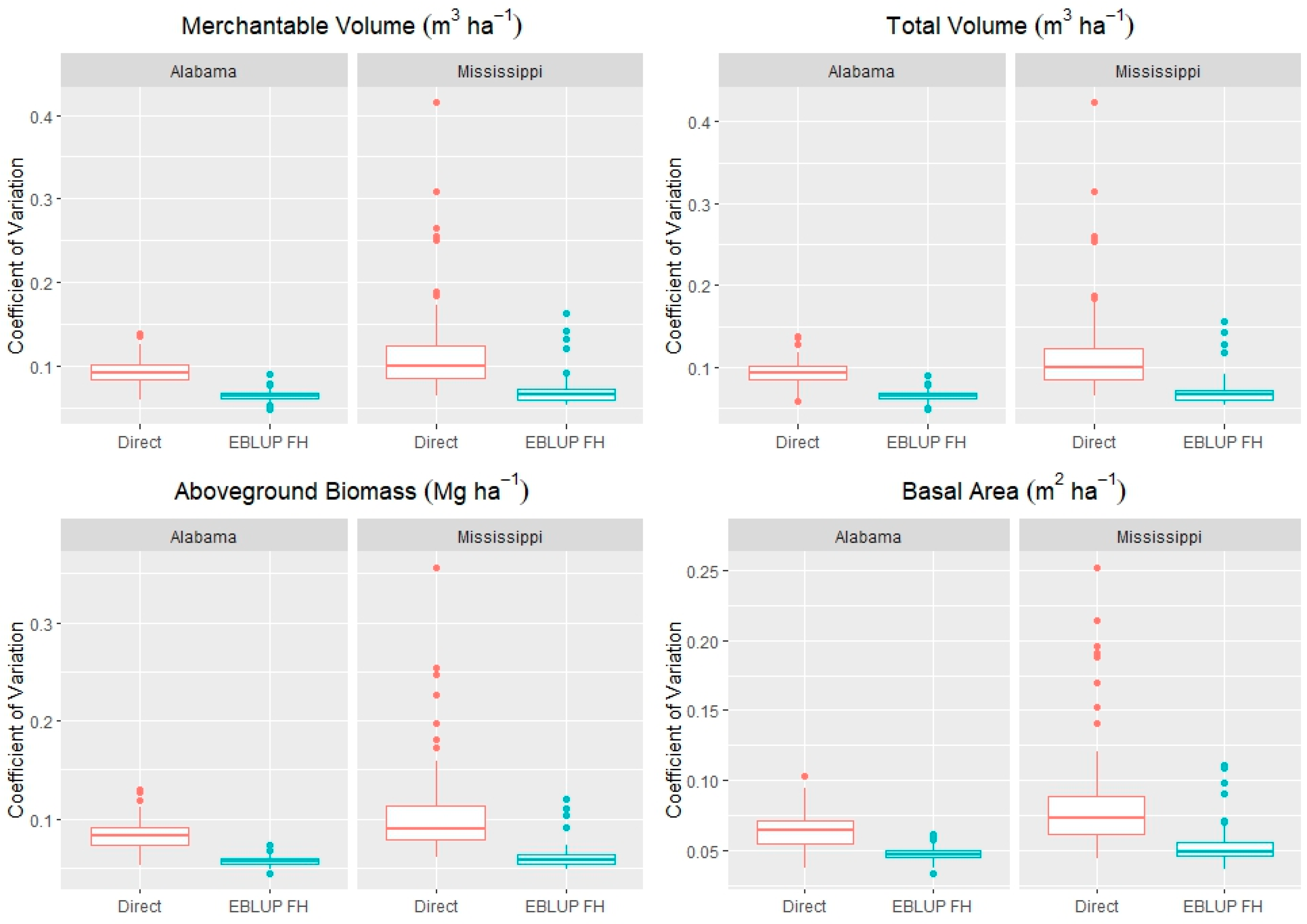
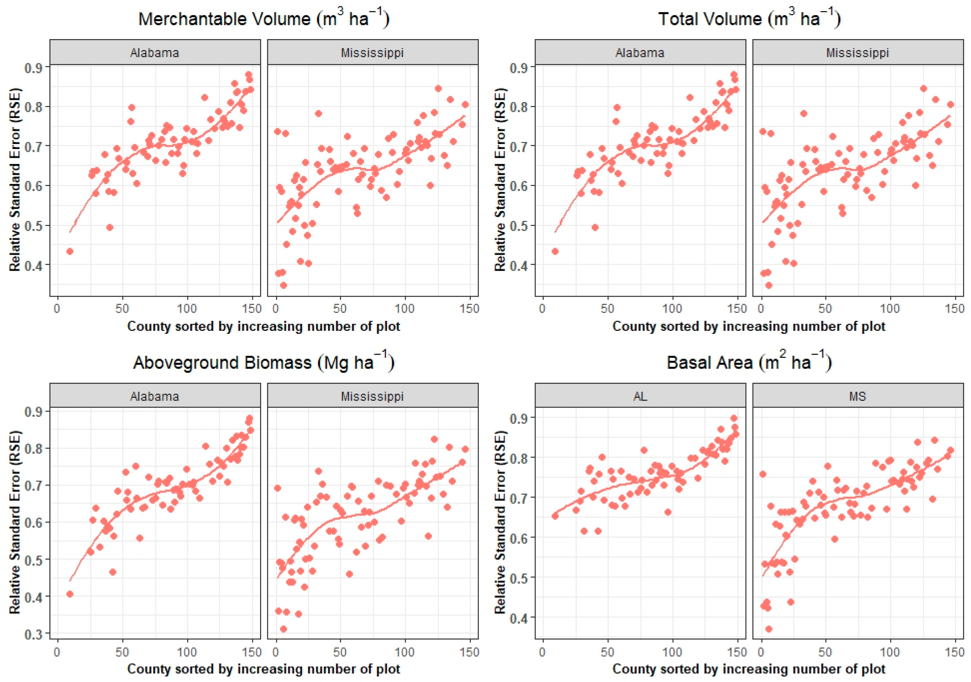
3.2. Performance of the Composite Estimator

The precision gained by the composite estimator is dependent on the relationship between the auxiliary information and the variable of interest.

Table 3. Comparison of the evaluation metrics of direct estimates with composite estimates for the multi-state models.

Variables of Interest	Direct Estimator			Composite Estimator
	Mean	CV	RMSE	Mean	CV	RMSE
AGB (Mg ha−1)	129.90	0.09	12.20	128.18	0.05	7.47
CVT (m3 ha−1)	155.83	0.10	16.15	153.20	0.06	10.31
CVM (m3 ha−1)	152.93	0.10	15.79	150.36	0.06	10.06
BA (m2 ha−1)	23.02	0.07	1.68	22.93	0.05	1.14

CV: Coefficient of Variation; RMSE: Root Mean Square Error; CVM: merchantable volume (m³ ha⁻¹); CVT: total volume (m³ ha⁻¹); AGB: aboveground biomass (Mg ha⁻¹); and BA: basal area (m² ha⁻¹).

shows the performance of the SAE composite estimator compared to FIA direct estimates based on the coefficient of variation (CV) and root mean square error (RMSE) for the multi-state models. At the county level, for all variables of interest, the composite estimates had more than a 30% reduction in their associated error compared to direct estimates. A comparison of the distribution of direct and composite estimates for the variables of interest by state is shown in Figure 4. The composite estimates of all variables of interest had lower variation than the direct estimates.

To determine the precision gained by the models at the county level, we calculated the relative standard error (RSE) metric.

Table 4. Comparison of the relative standard error of single and multi-state models at the county level.

Variables	Mississippi	Alabama	Multi-State
	RSE	RSE	RSE
AGB (Mg ha−1)	0.57 (0.28–0.91)	0.54 (0.30–0.97)	0.64 (0.31–0.88)
CVT (m3 ha−1)	0.57 (0.27–0.93)	0.54 (0.30–0.97)	0.67 (0.33–0.88)
CVM (m3 ha−1)	0.57 (0.28–0.93)	0.55 (0.32–0.97)	0.66 (0.34–0.87)
BA (m2 ha−1)	0.66 (0.35–0.90)	0.54 (0.35–1.08)	0.71 (0.36–0.90)

CVM: merchantable volume (m³ ha⁻¹); CVT: total volume (m³ ha⁻¹); AGB: aboveground biomass (Mg ha⁻¹); and BA: basal area (m² ha⁻¹). Relative Standard Error (RSE). The relative standard error is a measure of the precision gained by the composite estimator at the county level, calculated as the ratio of the root mean squared error of the composite estimator to the root mean squared error of the FIA direct estimator.

shows the precision gained based on the relative standard error (RSE) for single and multi-state models. There was a slight difference in the performance of the composite estimators for single and multi-state models. For all variables, the single-state model had a higher level of precision gained than the multi-state model. The multi-state model had a mean RSE value of 0.67 while single-state models had mean RSE values of 0.54 and 0.59 for Alabama and Mississippi, respectively.

Figure 5 shows the comparison of the coefficient of variation resulting from direct and composite estimates for each state. For both states, direct estimates had a higher degree of variability than the composite estimates. To further elucidate the accuracy gained by the composite estimators and the changes in the CV, we sorted (in an increasing manner) the CV of the direct estimates at the county level for both states (Figure 6). The plot shows the reduction and stability of the variation in the composite estimates around their mean. The variation is lower for composite estimates across all the variables and states than for the direct estimates. Figure 7 shows the precision gain as the number of sample plots increases. The relative standard error increases as the number of plots increases across all variables of interest. Across the two states, the gain in precision was relatively stable when counties had between 50 and 100 plots, and the precision gain was approximately 30% for all variables.

4. Discussion

Our analyses have demonstrated that derived information from optical (Landsat) and spaceborne lidar (GEDI) can improve the precision of national forest inventory estimates at small domains. Auxiliary information for small area estimation has been derived from various remote sensing sources, including satellite-based images, digital aerial photogrammetry, and aerial laser scanning [37]. This is because vegetation properties can be studied based on their reflection under the electromagnetic spectrum. Generally, composite bands used in vegetation analysis contain different band combinations such as short-wave infrared, near-infrared, red, and green bands. These bands have been reported to predict forest variables such as the variables of interest [38,39,40].

Across all variables of interest, derived GEDI metrics were significant predictors, especially the areas covered by trees in 25 m and 35 m height classes. This might be because tree height is significant in modeling tree volumes, aboveground biomass, and basal area [41]. Additionally, the height classes represent the most dominant tree species in the forests within the study area. The GEDI data version used in this study had improved footprint geolocation and prediction methods, making the forest structure information reliable at the specified spatial scale, especially when combined with national forest inventory data like the FIA.

The area-level SAE reduced errors for all variables of interest at single and multi-state levels. This is consistent with the findings of other area-level SAE studies [6,7,8,9,10,42]. The area-level SAE model relies on the regression synthetic estimates when the variance from the FIA direct estimate is high [8,19]. This implies that the model selection criterion is important as it directly impacts the accuracy and reliability of the estimates [34]. The Kullback information criteria (KICb2) used in model selection reduced the probability of selecting an incorrect model. This improved the SAE models’ predictions, resulting in a substantial reduction in the root mean square error given different sources of auxiliary information.

NFIs are designed to provide unbiased estimates at a large geographical scale, but are relatively limited due to the small samples available for sub-domain level estimation [13]. This justifies the high RMSE associated with the direct estimates at the county level for all variables of interest. However, at the county level, the SAE estimates for all variables of interest had error values that were approximately less than half of the direct estimates. The level of precision gained is significant and is comparable to other studies [8,17,26]. This demonstrates the significant potential of the developed area-level models in improving county-level FIA direct estimates on a large scale, particularly with the wall-to-wall availability and geographic coverage of both Landsat and GEDI data. However, careful consideration should be given to the tree species and the forest composition.

Airborne lidar is one of the most utilized auxiliary information sources for SAE [11]. However, airborne lidar is expensive, and the coverage is limited. By demonstrating the capabilities of GEDI data in improving the accuracy of forest inventory estimates at the county level, our work lays the foundations for future applications and modifications of small-area estimation techniques in forest monitoring and management. The accuracy achieved in this study conforms with several works that have been conducted using the SAE technique to improve the estimates of forest attributes at the area level. Cao et al. (2022) [8] reported an average precision gain that ranged between 19% and 30% for county-level estimates of forest volumes in three states. Although they used high-resolution (1 m and 5 m resampled to 10 m) auxiliary information derived from the canopy height metrics of National Agricultural Imagery Program (NAIP) images, the SAE model for merchantable and total volumes achieved a high level of precision. This shows that despite the spatial resolution (1 km) and the limited footprints of GEDI [32], combining it with Landsat can still be used to achieve a more precise estimate than the FIA direct estimates. While not the primary focus of this study, preliminary analysis using Sentinel-2 (10 m resolution) data showed no significant difference in the precision gained for the considered variables of interest. This aligns with the findings of [43] that there is a minimal effect of auxiliary information resolution on estimates and precision.

The probability of deriving statistically reliable estimates increases with a high number and larger plot size, particularly in diverse forest stands. The number of plots varies across states and counties; therefore, it was important to determine the precision gained with changes in the number of plots. From the analysis, the precision gained by the composite estimator decreases as the number of plots increases for all variables (RSE close to 1). This indicates that the model achieved approximately a 10% error reduction for counties with a large number of plots (100 or more). This is significant because the small area estimation assumption is that the small domain (county, in this study) lacks a sufficient sample size for a reliable estimate; thus, relying on auxiliary data to improve estimate precision. However, it seems the model relied on direct estimates for counties with a large number of plots, while significantly improving the estimates for counties with a smaller number of plots. Hence, the reason why counties with ≤50 plots had a significant precision gain (>30%), and those with ≥100 plots had a very low error reduction (<30%). Operationally, large-scale national inventories, such as FIA, could benefit from the SAE models tested here by improving their estimates, especially in states with lower sampling intensities. Additionally, both public and private stakeholders who depend on FIA data to develop their models or workflows can achieve higher accuracy. For example, modeling a specific tree species with FIA data can be improved to obtain estimates with lower variance using SAE models; industries that build their harvesting schedules or corroborate their datasets with FIA data can achieve higher precision. However, consideration should be given to the conditions of the forests, sample sizes, sampling design, and measurement error.

The auxiliary information combination developed for the area-level composite estimator in this study could be adopted or modified in modeling carbon trajectories, ecosystem resilience, and resistance at the county level. In addition, this study only considered merchantable and total cubic volumes, aboveground biomass, and basal area; however, the approach can be broadly applied to model other variables and ecosystem services. Furthermore, future research directions include evaluating the performance of SAE models using FIA data for specific forest types or small domains and incorporating additional indices and percentiles to enhance model accuracy and robustness.

5. Conclusions

This study evaluated the degree to which multisource remotely sensed data comprising spaceborne lidar (GEDI) and Landsat data can improve the precision of FIA estimates of forest variables at the county level using the area-level SAE. We used the Kullback information criterion (KICb2) to select the best model, which is specifically designed for variable selection in Fay–Herriot models. Based on the best model, both GEDI and Landsat metrics were significant predictors of all variables of interest. For the single and multi-state estimation, the area-level SAE models substantially increased the precision of the estimates at the county level for all variables of interest. This demonstrates the relevance of the area-based SAE model in improving forest variables at the county level, leveraging data from spaceborne active and passive sensors. Different FIA data users can utilize and modify metrics from Landsat and GEDI to improve forest attribute estimates at a larger scale without increasing sampling costs and efforts. Landowners and stakeholders utilizing FIA data can significantly benefit by improving the precision of their estimates, resulting in more accurate models and informed management decisions.

References

1. Bechtold, W.A.; Patterson, P.L. (Eds.) The Enhanced Forest Inventory and Analysis Program—National Sampling Design and Estimation Procedures; Gen. Tech. Rep. SRS-80; U.S. Department of Agriculture, Forest Service, Southern Research Station: Asheville, NC, USA, 2005; Volume 080, p. 85. [Google Scholar] [CrossRef]
2. Morin, R.S.; Pugh, S.A.; Liebhold, A.M.; Crocker, S.J. A regional assessment of emerald ash borer impacts in the Eastern United States: Ash mortality and abundance trends in time and space. In Proceedings of the Pushing Boundaries: New Directions in Inventory Techniques and Applications: Forest Inventory and Analysis (FIA) Symposium, Portland, OR, USA, 8–10 December 2015; pp. 233–236. [Google Scholar]
3. May, P.; McConville, K.S.; Moisen, G.G.; Bruening, J.; Dubayah, R. A spatially varying model for small area estimates of biomass density across the contiguous United States. Remote Sens. Environ. 2023, 286, 113420. [Google Scholar] [CrossRef]
4. Knott, J.A.; Liknes, G.C.; Giebink, C.L.; Oh, S.; Domke, G.M.; McRoberts, R.E.; Quirino, V.F.; Walters, B.F. Effects of outliers on remote sensing-assisted forest biomass estimation: A case study from the United States national forest inventory. Methods Ecol. Evol. 2023, 14, 1587–1602. [Google Scholar] [CrossRef]
5. Goerndt, M.E.; Monleon, V.J.; Temesgen, H. A comparison of small-area estimation techniques to estimate selected stand attributes using LiDAR-derived auxiliary variables. Can. J. For. Res. 2011, 41, 1189–1201. [Google Scholar] [CrossRef]
6. Goerndt, M.E.; Monleon, V.J.; Temesgen, H. Small-area estimation of county-level forest attributes using ground data and remote sensed auxiliary information. For. Sci. 2013, 59, 536–548. [Google Scholar] [CrossRef]
7. Coulston, J.W.; Green, P.C.; Radtke, P.J.; Prisley, S.P.; Brooks, E.B.; A Thomas, V.; Wynne, R.H.; E Burkhart, H. Enhancing the precision of broad-scale forestland removals estimates with small area estimation techniques. Forestry 2021, 94, 427–441. [Google Scholar] [CrossRef]
8. Cao, Q.; Dettmann, G.T.; Radtke, P.J.; Coulston, J.W.; Derwin, J.; Thomas, V.A.; Burkhart, H.E.; Wynne, R.H. Increased Precision in County-Level Volume Estimates in the United States National Forest Inventory With Area-Level Small Area Estimation. Front. For. Glob. Change 2022, 5, 769917. [Google Scholar] [CrossRef]
9. Green, P.C.; Burkhart, H.E.; Coulston, J.W.; Radtke, P.J. A novel application of small area estimation in loblolly pine forest inventory. Forestry 2019, 93, 444–457. [Google Scholar] [CrossRef]
10. Green, P.C.; Hogg, D.W.; Watson, B.; Burkhart, H.E. Small Area Estimation in Diverse Timber Types Using Multiple Sources of Auxiliary Data. J. For. 2022, 120, 646–659. [Google Scholar] [CrossRef]
11. Dettmann, G.; Radtke, P.; Coulston, J.; Green, P.; Wilson, B.; Moisen, G. Review and Synthesis of Estimation Strategies to Meet Small Area Needs in Forest Inventory. Front. For. Glob. Change 2022, 5, 813569. [Google Scholar] [CrossRef]
12. Mandallaz, D.; Breschan, J.; Hill, A. New regression estimators in forest inventories with two-phase sampling and partially exhaustive information: A design-based monte carlo approach with applications to small-area estimation. Can. J. For. Res. 2013, 43, 1023–1031. [Google Scholar] [CrossRef]
13. Frescino, T.S.; McConville, K.S.; White, G.W.; Toney, J.C.; Moisen, G.G. Small Area Estimates for National Applications: A Database to Dashboard Strategy Using FIESTA. Front. For. Glob. Change 2022, 5, 779446. [Google Scholar] [CrossRef]
14. Gomez-Rubio, V.; Best, N.; Richardson, S. A Comparison of Different Methods for Small Area Estimation; Working Paper; ESRC National Centre for Research Methods: Southampton, UK, 2009; Available online: https://eprints.ncrm.ac.uk/id/eprint/743/ (accessed on 1 September 2022).
15. USDA Forest Service. Forests of Mississippi, 2020. 2022. Available online: https://www.fs.usda.gov/treesearch/pubs/64765 (accessed on 5 July 2025).
16. Woudenberg, S.W.; Conkling, B.L.; O’connell, B.M.; Lapoint, E.B.; Turner, J.A. The Forest Inventory and Analysis Database: Database Description and Users Manual Version 4.0 for Phase 2; United States Department of Agriculture, Forest Service, Rocky Mountain Research Station: Fort Collins, CO, USA, 2010. [Google Scholar]
17. Magnussen, S.; Mandallaz, D.; Breidenbach, J.; Lanz, A.; Ginzler, C. National forest inventories in the service of small area estimation of stem volume. Can. J. For. Res. 2014, 44, 1079–1090. [Google Scholar] [CrossRef]
18. Hill, A.; Massey, A.; Mandallaz, D. The R Package forestinventory: Design-Based Global and Small Area Estimations for Multiphase Forest Inventories. J. Stat. Softw. 2021, 97, 1–40. [Google Scholar] [CrossRef]
19. Rao, J.N.; Molina, I. Small Area Estimation; John Wiley & Sons: Hoboken, NJ, USA, 2015. [Google Scholar]
20. Hidiroglou, M. Small-Area Estimation: Theory and Practice. In JSM Proceedings, Survery Research Methods Section; American Statistical Association: Alexandria, VA, USA, 2007. [Google Scholar]
21. Costa, A.; Ventura, E.; Satorra, A. An Empirical Evaluation of Small Area Estimators. SORT (Stat. Oper. Res. Trans.) 2003, 27, 113–136. [Google Scholar] [CrossRef]
22. McRoberts, R.E. Estimating forest attribute parameters for small areas using nearest neighbors techniques. For. Ecol. Manag. 2012, 272, 3–12. [Google Scholar] [CrossRef]
23. Fay, R.E.; Herriot, R.A. Estimates of Income for Small Places: An Application of James-Stein Procedures to Census Data. J. Am. Stat. Assoc. 1979, 74, 269–277. [Google Scholar] [CrossRef]
24. Battese, G.E.; Harter, R.M.; Fuller, W.A. An Error-Components Model for Prediction of County Crop Areas Using Survey and Satellite Data. J. Am. Stat. Assoc. 1988, 83, 28–36. [Google Scholar] [CrossRef]
25. Brosofske, K.D.; Froese, R.E.; Falkowski, M.J.; Banskota, A. A Review of Methods for Mapping and Prediction of Inventory Attributes for Operational Forest Management. For. Sci. 2014, 60, 733–756. [Google Scholar] [CrossRef]
26. Breidenbach, J.; Astrup, R. Small area estimation of forest attributes in the Norwegian National Forest Inventory. Eur. J. For. Res. 2012, 131, 1255–1267. [Google Scholar] [CrossRef]
27. Goerndt, M.E.; Wilson, B.T.; Aguilar, F.X. Comparison of small area estimation methods applied to biopower feedstock supply in the Northern U.S. region. Biomass Bioenergy 2019, 121, 64–77. [Google Scholar] [CrossRef]
28. McRoberts, R.E.; Næsset, E.; Gobakken, T. Inference for lidar-assisted estimation of forest growing stock volume. Remote Sens. Environ. 2013, 128, 268–275. [Google Scholar] [CrossRef]
29. Gomillion, C.G.; Norrell, R.J. Alabama. In Encyclopedia Britannica; Encyclopedia Britannica, Inc.: Chicago, IL, USA, 2023. [Google Scholar]
30. Alabama Forestry Commission. Alabama Forest Road Map 2020; Alabama Forestry Commission: Montgomery, AL, USA, 2020. Available online: https://forestry.alabama.gov/Pages/Management/Forms/Forest_Action_Plan.pdf (accessed on 5 July 2025).
31. VanderSchaaf, C. Obtaining Biomass/Volume/Carbon Estimates Using EVALIDator Version 2.0.3 | Mississippi State University Extension Service. Available online: https://extension.msstate.edu/sites/default/files/publications/publications/P3830_web.pdf (accessed on 9 May 2023).
32. Potapov, P.; Li, X.; Hernandez-Serna, A.; Tyukavina, A.; Hansen, M.C.; Kommareddy, A.; Pickens, A.; Turubanova, S.; Tang, H.; Silva, C.E.; et al. Mapping global forest canopy height through integration of GEDI and Landsat data. Remote Sens. Environ. 2021, 253, 112165. [Google Scholar] [CrossRef]
33. Dubayah, R.; Luthcke, S.; Sabaka, T.; Nicholas, J.; Preaux, S.; Hofton, M. GEDI L3 Gridded Land Surface Metrics, version 1; ORNL DAAC: Oak Ridge, TN, USA, 2021. [Google Scholar] [CrossRef]
34. Marhuenda, Y.; Morales, D.; del Carmen Pardo, M. Information criteria for Fay–Herriot model selection. Comput. Stat. Data Anal. 2014, 70, 268–280. [Google Scholar] [CrossRef]
35. Kreutzmann, A.-K.; Pannier, S.; Rojas-Perilla, N.; Schmid, T.; Templ, M.; Tzavidis, N. The R Package emdi for Estimating and Mapping Regionally Disaggregated Indicators. J. Stat. Softw. 2019, 91, 1–33. [Google Scholar] [CrossRef]
36. R Core Team. R: A Language and Environment for Statistical Computing; R Foundation for Statistical Computing: Vienna, Austria, 2023; Available online: https://www.R-project.org/ (accessed on 3 September 2023).
37. Zhang, S.; Vega, C.; Deleuze, C.; Durrieu, S.; Barbillon, P.; Bouriaud, O.; Renaud, J.-P. Modelling forest volume with small area estimation of forest inventory using GEDI footprints as auxiliary information. Int. J. Appl. Earth Obs. Geoinform. 2022, 114, 103072. [Google Scholar] [CrossRef]
38. Astola, H.; Häme, T.; Sirro, L.; Molinier, M.; Kilpi, J. Comparison of Sentinel-2 and Landsat 8 imagery for forest variable prediction in boreal region. Remote Sens. Environ. 2019, 223, 257–273. [Google Scholar] [CrossRef]
39. Chrysafis, I.; Mallinis, G.; Siachalou, S.; Patias, P. Assessing the relationships between growing stock volume and Sentinel-2 imagery in a Mediterranean forest ecosystem. Remote Sens. Lett. 2017, 8, 508–517. [Google Scholar] [CrossRef]
40. Antropov, O.; Rauste, Y.; Tegel, K.; Baral, Y.; Junttila, V.; Kauranne, T.; Hame, T.; Praks, J. Tropical forest tree height and above ground biomass mapping in Nepal using Tandem-X and ALOS PALSAR data. In Proceedings of the IGARSS 2018-2018 IEEE International Geoscience and Remote Sensing Symposium, Valencia, Spain, 22–27 July 2018; IEEE: New York, NY, USA, 2018; pp. 5334–5336. [Google Scholar]
41. Asigbaase, M.; Dawoe, E.; Abugre, S.; Kyereh, B.; Nsor, C.A. Allometric relationships between stem diameter, height and crown area of associated trees of cocoa agroforests of Ghana. Sci. Rep. 2023, 13, 14897. [Google Scholar] [CrossRef]
42. Temesgen, H.; Mauro, F.; Hudak, A.T.; Frank, B.; Monleon, V.; Fekety, P.; Palmer, M.; Bryant, T. Using Fay–Herriot Models and Variable Radius Plot Data to Develop a Stand-Level Inventory and Update a Prior Inventory in the Western Cascades, OR, United States. Front. For. Glob. Change 2021, 4, 745916. [Google Scholar] [CrossRef]
43. Green, P.C.; Burkhart, H.E.; Coulston, J.W.; Radtke, P.J.; Thomas, V.A. Auxiliary information resolution effects on small area estimation in plantation forest inventory. Forestry 2020, 93, 685–693. [Google Scholar] [CrossRef]
Figure 1. Map of the study area: (A) the southern states of the United States; (B) states of Alabama and Mississippi with the publicly reported (fuzzed and swapped) FIA plot locations.
Remotesensing 17 02407 g001
Figure 2. Graphical representation of data sources, variables of interest, and the computer programs used in this study.
Remotesensing 17 02407 g002
Figure 3. Fay–Herriot composite estimates (EBLUP) of county-level forest attributes compared to FIA direct estimates by state. The blue line represents the 1:1 relationship between the composite and direct estimates, while the red line is the regression line based on the model.
Remotesensing 17 02407 g003
Figure 4. Comparison of the distribution of composite estimates to the direct estimates by state.
Remotesensing 17 02407 g004
Figure 5. Comparison of the coefficient of variation between the composite and the direct estimates by state for all the variables of interest.
Remotesensing 17 02407 g005
Figure 6. Changes in the coefficient of variation between the composite and the direct estimates by state for all the variables of interest.
Remotesensing 17 02407 g006
Figure 7. The precision gain by the composite estimator based on increasing plot size by state for all the variables of interest.
Remotesensing 17 02407 g007