Surface Reconstruction Planning with High-Quality Satellite Stereo Pairs Searching

Abstract

Advancements in remote sensing technology have remarkably enhanced the 3D Earth surface reconstruction, which is pivotal for applications such as disaster relief, emergency management, and urban planning, etc. Although satellite imagery offers a cost-effective and extensive coverage solution for 3D reconstruction, the quality of the resulted digital surface model (DSM) heavily relies on the choice of stereo image pairs. However, current approaches of stereo Earth observation still employ a post-acquisition manner without sophisticated planning in advance, causing inefficiencies and low reconstruction quality. This paper introduces a novel quality-driven planning method for satellite stereo imaging, aiming at optimizing the search of stereo pairs to achieve high-quality 3D reconstruction. Moreover, a regression model is customized and incorporated to estimate the reconstructed point cloud geopositioning quality, based on the enhanced features of possible Earth-imaging opportunities. Experiments conducted on both real satellite images and simulated constellation data demonstrate the efficacy of the proposed method in estimating reconstruction quality beforehand and searching for optimal stereo pair combinations as the final satellite imaging schedule, which can improve the stereo quality significantly.

1. Introduction

The continuous development of remote sensing technology has facilitated Earth 3D surface reconstruction, which is widely used in disaster prevention and mitigation, emergency preparation, urban planning, etc. This reconstruction can be achieved by applying geometric analysis after the acquisition of satellite photogrammetric images with proper intersection angles between them. Compared to UAV aerial imagery, satellite imagery is more cost-effective in covering a wider geographic area, and it can capture Earth observation data in a shorter period, thus acquiring a 3D reconstructed view of any target area on a global scale [1]. In addition, the high spatial resolution of satellite images makes it possible to reconstruct high-quality 3D scene information from these images [2,3,4], for which stereo matching algorithms need to be applied to generate a dense 3D point cloud and DSM.

To recover the detailed 3D information of scenes such as cities, streetscapes, and buildings, at least two high-resolution images are needed to provide accurate stereo matching. For example, Li et al. proposed a double propagation stereo matching (DPSM) method for urban 3D reconstruction from stereo-rectified satellite images, which leverages superpixel-based geometric models and three similarity metrics to optimize disparity estimation, while demonstrating superior performance in preserving depth discontinuities and handling occlusions [5]. Yang et al. introduced a generalized stereo matching method that addresses challenges such as the radiation difference and small ground feature difference in satellite images [6]. Their approach utilizes hierarchical graph structure consistency and iterative optimization to improve matching accuracy in urban 3D scene reconstruction. Similarly, Orsingher et al. proposed a comprehensive pipeline for image-based 3D reconstruction of urban scenarios, employing PatchMatch Multi-View Stereo (MVS) techniques [7]. Furthermore, Stucker and Schindler developed ResDepth, a deep residual prior for 3D reconstruction from high-resolution satellite images [8]. This convolutional neural network refines initial stereo digital surface models by conditioning the refinement on the images, effectively improving the quality of 3D reconstructions in urban settings. These studies underscore the ongoing efforts to enhance 3D reconstruction methodologies by integrating advanced stereo matching techniques and machine learning approaches.

Currently, satellite observation of the Earth mainly relies on the push-broom mode to obtain remote sensing images, but this method is prone to errors in stereo correction [9]. The quality of 3D content generation using satellite image pairs can be affected by many factors and is still questionable and unpredictable. For example, most of the literature focuses on the effect of the intersection angles (base–height ratios) on the dense matching results primarily for in-track satellite stereo pairs [10,11]. Instead, Qin R et al. pointed out that the intersection angle is insufficient for stereo pair selection and emphasized the importance of sun-angle difference in determining stereo pair quality [12]. Moreover, Facciolo G et al. analyzed the correlation of the angle between the views, maximum incidence angle, and time difference between the acquisitions, with the quality of DSM [13]. The authors in [14] suggested that the stereo convergence angle should have a value between $5^{\circ }$ and ${15}^{\circ }$, and the difference in sun angles between the two images should be below $25$–${30}^{\circ }$ for satisfactory stereo constructions. Though these conclusions can be useful in guiding multi-view satellite image reconstruction to improve the quality of DSM, such work is carried out in an acquisition–selection manner, i.e., the satellite images are first acquired and then selected to form the stereo pairs. There is still a lack of quantitative algorithms to generate image acquisition plans aiming at high-quality Earth surface 3D reconstruction, so as to decrease redundant remote sensing and data transmission which is usually costly in urgent cartography for emergency management.

In this paper, we propose a novel stereo reconstruction planning method based on quality-driven satellite image pair searching. First, for each pair of stereo images, the quality of the DSM generated using them is calculated by building an estimation model and taking into account various factors. Second, the quality-driven stereo sensing planning method is modeled and solved, by predicting quality values using the quality estimation model while searching for optimal stereo image pairs with a metaheuristic algorithm. Finally, the proposed method is evaluated on extensive satellite orbital simulations aligned with a realistic multi-view stereo dataset. The experimental results show that the quality of the stereo surface can be significantly improved using the quality estimation and task planning method to search for optimal satellite image combinations. To the best of our knowledge, such remote sensing task planning to support high-quality DSM has not been conducted before. The contributions of this paper are as follows:

• A regression method is customized to provide accurate estimation of DSM quality using real reconstructed point cloud geopositioning errors for training. Feature enhancement and selection are applied to retain key factors that contribute significantly to the quality prediction.
• Multi-objective satellite image acquisition planning is modeled to maximize the 3D reconstruction quality while balancing with task quantity and timeliness, which is NP-hard and solved efficiently with constrained optimization algorithms.
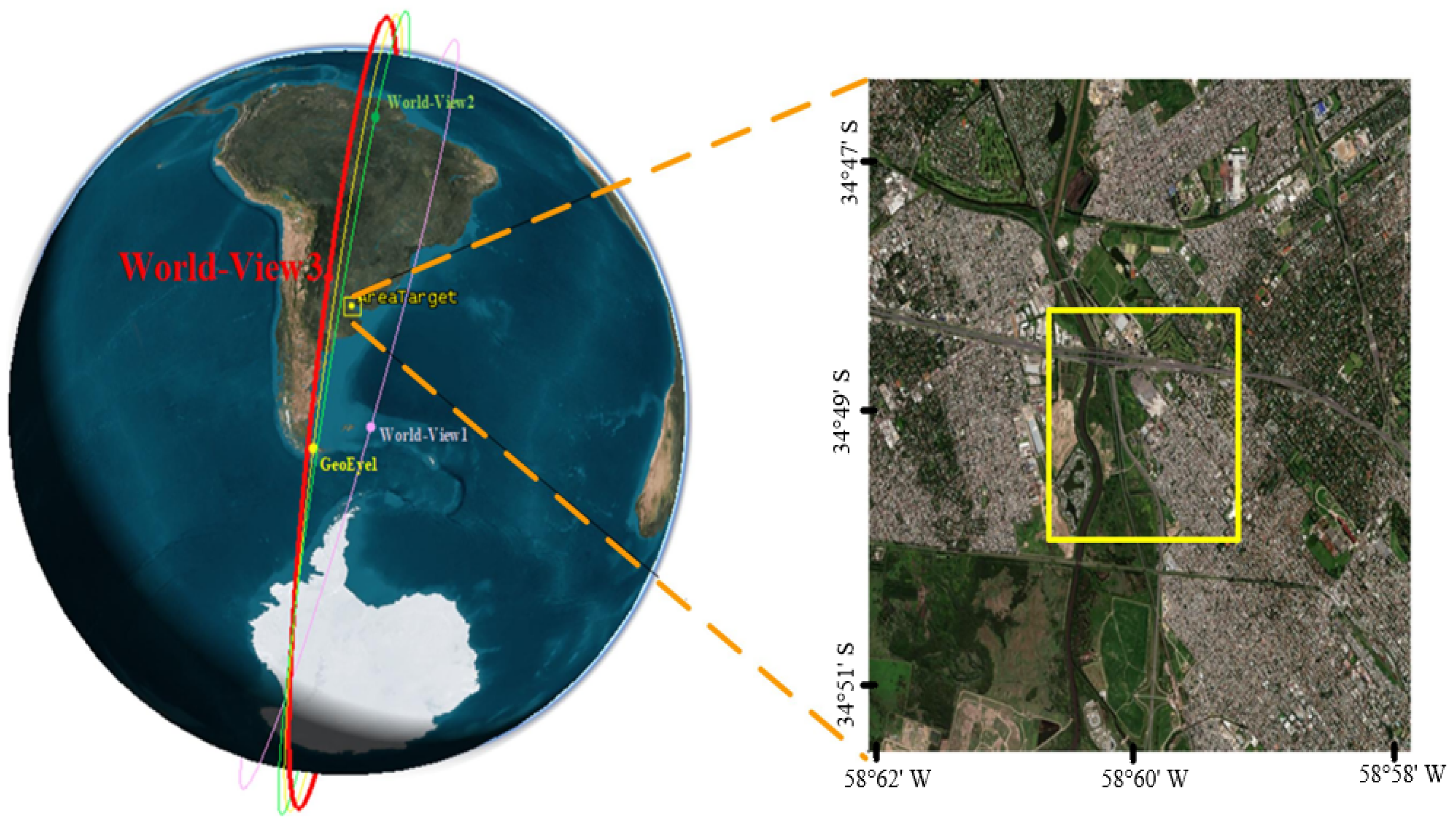
• The orbits of satellite WorldView-3 and its constellation are both simulated and aligned with the real stereo image dataset to form a comprehensive dataset for quality-driven stereo sensing task planning evaluation, which is to be released to the community.

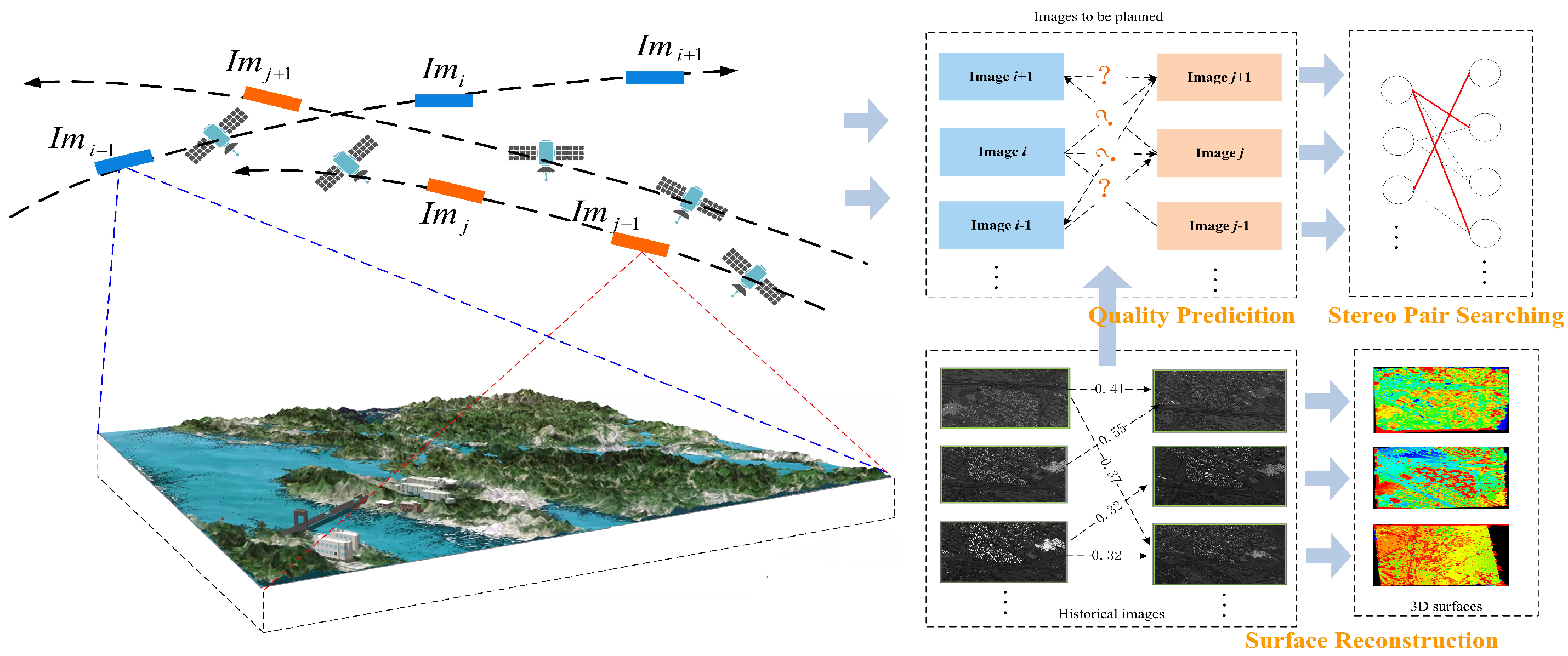
2. Motivation and Method Overview

2.1. Surface Reconstruction Planning Description

The existing satellite photography focuses on observing point or area targets [15], and the planning for this kind of task is to provide the maximized fulfillment of target observations. Because there are usually many possible imaging opportunities for satellites, represented as time windows in their orbits, the role of planning is to choose the time windows and provide the final imaging schedule which maximizes the overall profits. Though image quality is also considered as one of the objectives, such as in [16,17,18], they still tackle traditional satellite imaging tasks. The authors in [19] formalize the quality of stereo imaging tasks as one objective and its variance as another. However, the image quality directly affected by satellite attitude is considered as the 3D reconstruction quality, i.e., calculated as the result of the pitch and roll angles of the satellite, which is similar to reference [18], where the satellite attitude is converted to one imaging angle to represent quality.

Assuming the images captured for all possible visible time windows $VTW$ are denoted as $IM$, each image $i{m}_i$ has its attributes of $a_i$ including off-nadir angle, solar elevation angle, solar azimuth angle, etc., where $1\le i\le N$ and N is the total number of imaging opportunities. Without losing generality, the single-target 3D reconstruction from two images is a function $f(i{m}_i,i{m}_j):IM\times IM\to S$ to map from an image pair to a stereo reconstruction. The task of planning here is to search for optimal pairs of images which lead to high-quality 3D reconstructions. Because planning is a decision making process which can only be implemented before imaging is actually fulfilled, the quality of reconstruction from an arbitrary image pair should be estimated accurately beforehand, according to their attributes of $a_i$ and $a_j$ which can be calculated according to the satellite orbit.

However, the influence of different attributes and their intersections on reconstruction quality is unclear and hard to quantify. Even with the predicted quality, how to search for optimized stereo combinations from a large number of imaging opportunities is not addressed. This is especially challenging for 3D reconstruction with large constellations, to which the quality-driven planning method proposed in this paper can be applied.

2.2. Framework of Quality-Driven Stereo Planning Algorithm

As previously discussed, the estimation of stereo reconstruction quality in advance is an essential premise for quality-driven planning. In this paper, we propose to learn a regression model to quantify this value from historical data by correlating 3D reconstruction results with the attributes of time windows, as shown in Figure 1. The possible opportunities of image shooting are calculated according to satellite orbital dynamics and are illustrated as slices in the orbits. While historical data contain images which can be used to determine the final reconstruction quality for estimation model learning, the future tasks to be planned can only have the time windows with their attributes as input. The images to be planned corresponding to the time slices in orbits are depicted with the same color of blue or orange, representing the images to be captured with different satellites in the constellation.

As shown in Figure 1, the proposed algorithm consists of three main components including 3D surface reconstruction, quality prediction, and stereo pair searching. The role of surface reconstruction is to accurately recover a realistic 3D Earth surface using satellite photogrammetric images as input. Though progress has continuously been made in 3D remote sensing by employing state-of-the-art computer vision technologies, the reconstruction outcome highly depends on the original quality and attributes of the satellite image pair, which needs to be carefully planned, for which the estimation of quality is essential and can be learned from historical DSM reconstruction results. For historical images in Figure 1, pair-wise image combinations are connected, and the DSM accuracy of each pair can be compared to the ground-truth 3D model to provide quality values which are depicted as the edge weights of pair-wise links in historical images. The detailed attributes of each image’s time window are then mapped to the calculated quality to learn the regression model for further predictions of future tasks whose quality of 3D reconstruction is unknown beforehand. In this procedure, a CatBoost algorithm is employed with customized feature enhancement and selection to fulfill accurate quality prediction. The planning model can then be modeled with the overall quality as one objective, and the optimal combinations of imaging opportunities can be found by searching for high objective fitness, so as to achieve a quality-driven planning method. As shown in Figure 1, given the constraints such as satellite maneuvering time, the searching of stereo pairs can be solved as a constrained combinatorial optimization problem which is NP-hard. In the proposed planning, multi-objectives including reconstruction quality as well as task quantity and timeliness are optimized to generate a feasible imaging schedule for satellites to execute. In this way, high-precision reconstruction with appropriate image pairs can be obtained, thus significantly improving the quality and efficiency of 3D reconstruction.

3. Quality Estimation of Earth Surface Reconstruction

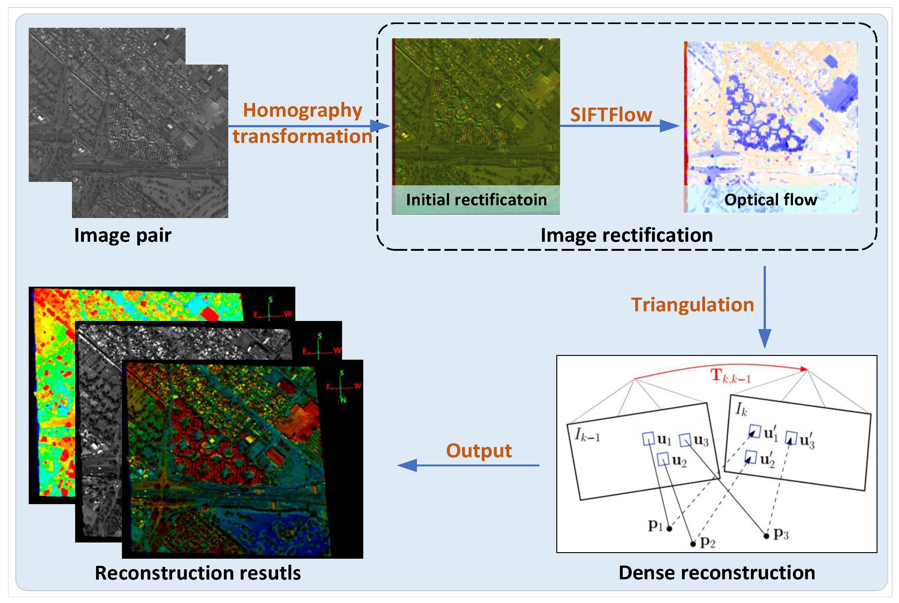
3.1. Earth Surface 3D Reconstruction

In this paper, we utilize a classical 3D reconstruction pipeline to generate point clouds from pairs of images along with their associated camera poses. This pipeline consists of two main steps of feature-based image rectification and triangulation-based dense reconstruction [2] as shown in Figure 2. Given that space-borne imaging platforms are typically positioned at high elevations, the objects on the ground can be reasonably approximated as being coplanar. Therefore, homography transformation is employed as the core method to establish geometric relationships between the two image planes in each stereo pair.

During the image rectification, Scale-Invariant Feature Transform (SIFT) is a commonly used method [20]. First, SIFT is employed to detect and describe feature points in a pair of images A and B. For image A, we consider it as the reference image for rectification and set its homography matrix $H_1$ to the identity matrix. As for image B, the homography matrix $H_2$ relative to image A is estimated based on feature matching. Sparse feature point sets are selected as initial inputs, combined with the Random Sample Consensus (RANSAC) algorithm for robust estimation [21]. Through iterative solving, the optimal homography matrix $H_2$ is obtained, which is then applied to geometrically transform the feature points from image B to align with that of image A. This process can be described as $x_A=H_2·x_B$, where $x_A$ and $x_B$ denote the homogeneous coordinates of feature points from images A and B, respectively. Due to the inability of homography transformation to handle the rectification of local pixels with significant spatial differences, the SiftFlow algorithm is employed for dense optical flow estimation to refine the initial rectification (top-right dashed box in Figure 2), which can effectively capture subtle motion information between images to improve the coverage of rectification [22]. Afterwards, the dense matching results of two-dimensional coordinates, excluding occlusion effects, are obtained to support the triangulation-based dense reconstruction.

Absolute scale information is necessary for the task of 3D reconstruction from satellite images. The RPC (Rational Polynomial Coefficients) model is widely used in optical satellite imagery because it not only incorporates scale information but also allows for the description of complex acquisition systems without depending on physical modeling specific to the satellite [23]. Each RPC is defined by a 3D–2D projection function to map Earth coordinates to image pixels and its inverse function, which maps image pixels back to Earth coordinates.

After the rectification, the dense triangulation is conducted for the generation of a high-quality dense reconstruction, which generates the 3D coordinates of ground points by solving the intersection of back-projected rays from matched pixel pairs obtained in the previous step. First, the pixel coordinates are converted to normalized coordinates according to the RPC model. Using these normalized coordinates, an initial estimation of the 3D point position is derived through linear least squares fitting. This estimation is then iteratively refined by minimizing the reprojection error, which is the difference between the observed pixel coordinates and the predicted coordinates obtained by projecting the estimated 3D point back onto the image planes. The process continues until the reprojection error converges to a sufficiently small value or the maximum number of iterations is reached. Once the dense triangulation is completed, the reconstruction results are output, which accurately represent the 3D structure of the scene.

3.2. Regression Model for Quality Estimation

The DSM reconstruction method can generate 3D models based on the captured satellite image pairs. The reconstruction precision can then be compared to the 3D model ground truth to quantify the quality, based on which the quality prediction model can be trained. In this study, the DSM error is used as an assessment metric of reconstruction quality. It is determined by calculating the mean square error (MSE) between the ground truth and the DSM values reconstructed using the algorithm in Section 3.1. The smaller MSE value means the reconstruction result is closer to the ground truth. Different from other regression tasks, the features of a pair of imaging time windows are highly correlated and have complex impacts on the reconstruction quality, depending on not only the raw features but also their intersections. In this section, a CatBoost-based learning method is proposed with feature enhancement and then trained with feature selection. CatBoost is an efficient Gradient Boosting Decision Tree (GBDT) framework with the advantage in significantly improving model performance and stability, through a series of optimization techniques such as ordered boosting, category feature coding, and overfitting reduction [24].

To improve the effectiveness of the regression model, we perform several preprocessing steps to further adapt CatBoost to the problem of stereo pair quality estimation. First, we enrich the dataset with feature enhancement to ensure that the model is capable of dealing with the rich and highly relevant feature inputs. Second, we perform feature selection using LASSO (Least Absolute Shrinkage and Selection Operator) regression to identify the most predictive features from the enhanced feature set [25].

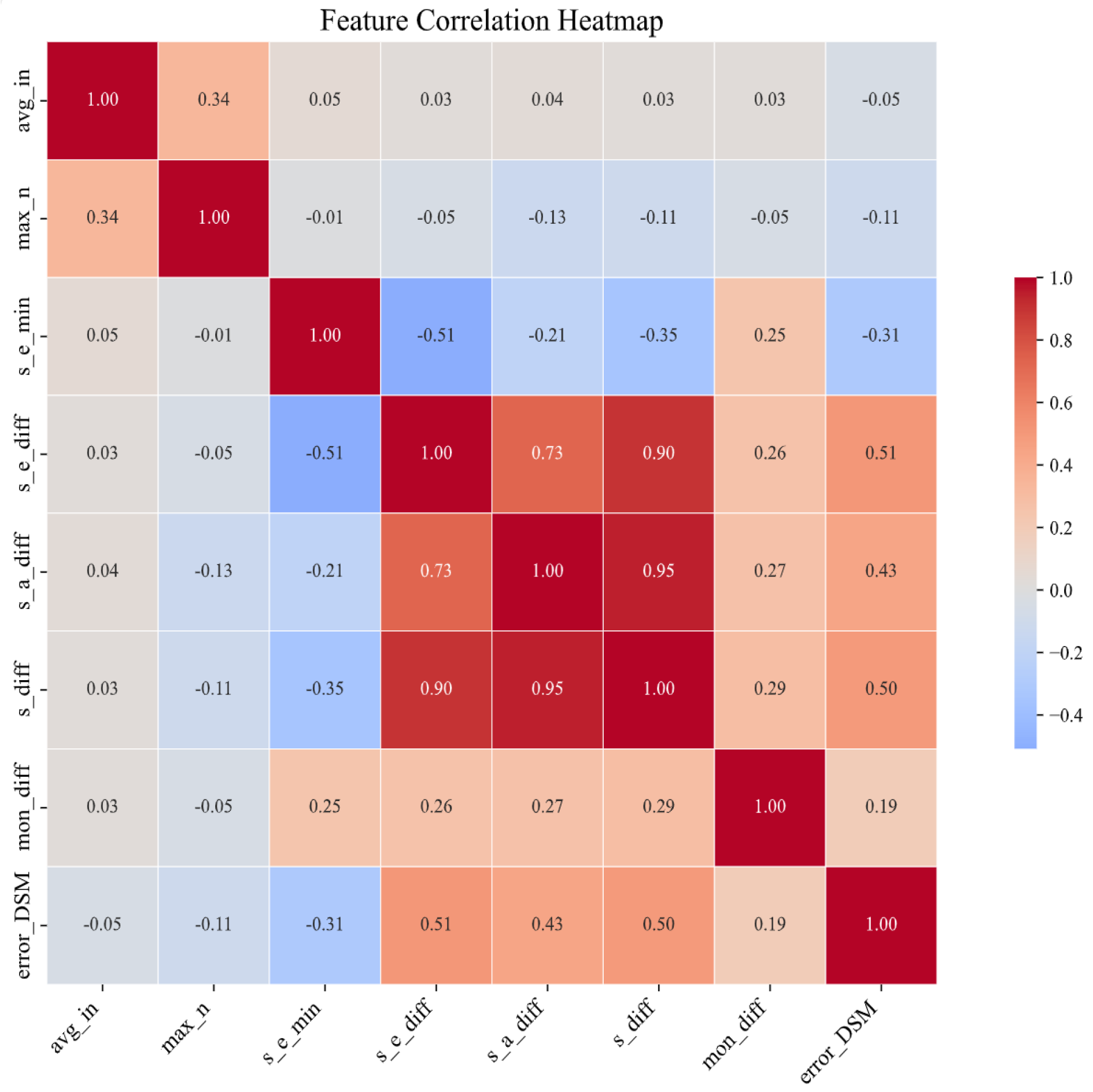
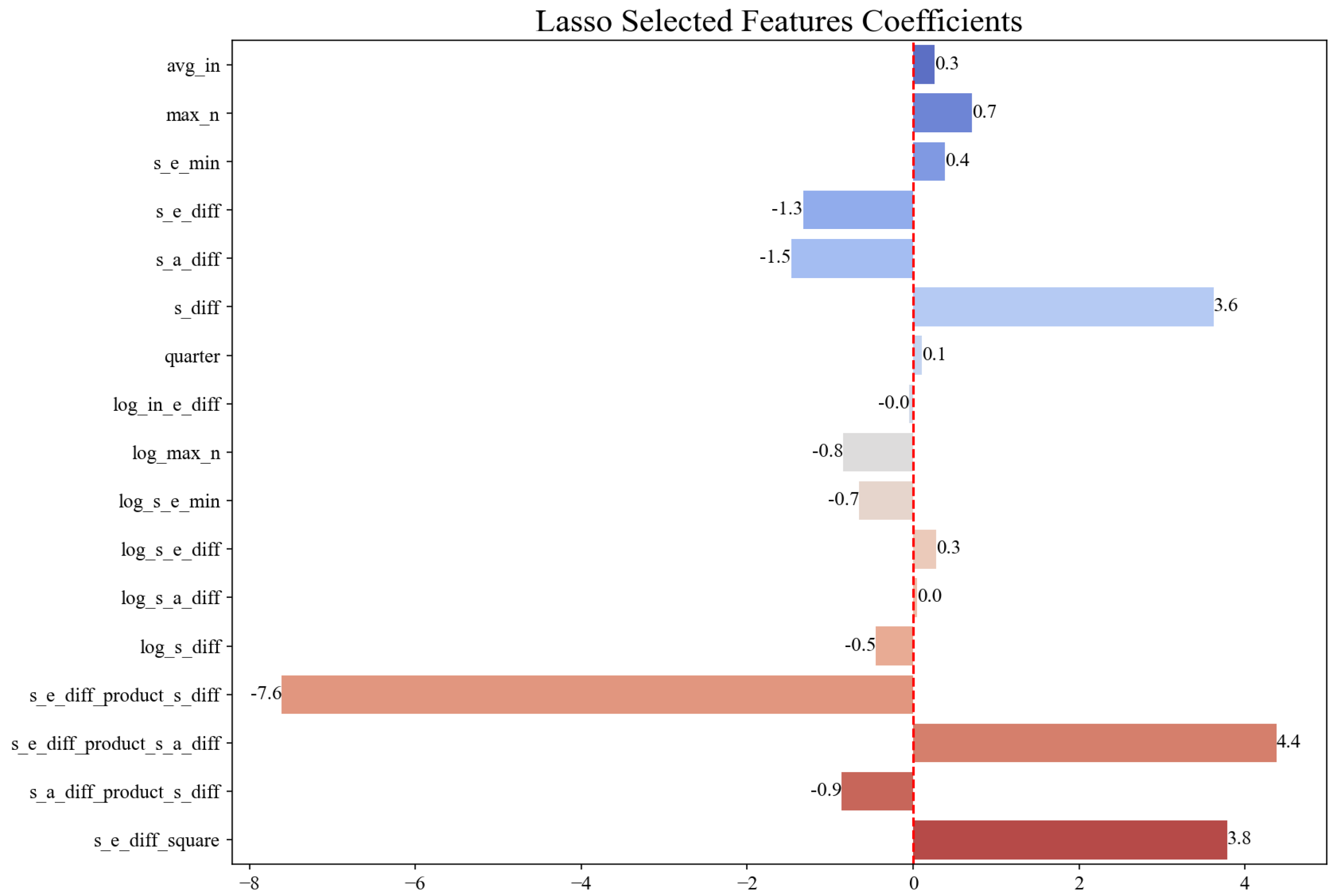
3.2.1. Selection for High-Dimensional Features

The characterization features for quality estimation consist of satellite imaging meta-parameters such as solar elevation angle, solar azimuth angle, time interval, intersection angle, etc., leading to a multi-dimensional regression problem. Because these raw parameters have different influences on the final accuracy of 3D reconstruction, a new form of features is constructed by combining the raw features of an image pair. For example, the difference of two solar azimuth angles is an intersection of two raw features, leading to a new representation. Besides the difference, the operations of the minimum, maximum, root of sum of squares, etc., are also applied to enhance the features. Because not all constructed features are equally important, the Pearson Correlation Coefficient map is calculated for filtering and enhancing the features as shown in Figure 3, in which various features are depicted and compared.

From Figure 3 we can find that the features derived from solar elevation and azimuth angles are more strongly correlated with DSM accuracy, including $s\_a\_diff$ (difference of sun azimuth angle), $s\_e\_diff$ (difference of sun elevation angle), etc., which will be further utilized for feature enhancement. Logarithmic transformation is applied to these chosen parameters to capture the nonlinear relationships [26,27,28]. The transformed features are then appended to the previous features. These efforts construct a richer and more diverse feature space, thus providing a more solid dataset for model training, to better capture complex patterns in the data and improve the quality estimation accuracy, together with the LASSO-based feature selection.

LASSO can automate feature selection by introducing an absolute value-based penalty term (L1 regularization) on top of the traditional least squares method, which not only effectively shrinks the model coefficients, but also reduces unimportant feature coefficients to zeros [25]. This characteristic makes LASSO well suited to deal with high-dimensional data, reducing overfitting while improving the interpretive and predictive performance of the model. Inspired by reference [29], the optimization for quality linear estimation can be formalized as follows:

$$\underset{C\in {\mathbb{R}}^d}{min}{\displaystyle \frac{1}{2}}{∥Y-X^{T}C∥}_2^2+\lambda {∥C∥}_1$$

(1)

where $C={[c_1,\dots ,c_d]}^T$ is the regression coefficient vector, and $c_k$ is the regression coefficient for the k-th feature; $1\le k\le d$. $\lambda {∥C∥}_1$ is a penalty specific to regression, using L1 norm ${∥·∥}_1$. This encourages some coefficients to become 0 to achieve the effect of feature selection. $\lambda$ is the regularization parameter and controls the penalty intensity. In Equation (1), each sample $({\mathbf{x}}_i,y_i)$ ($1\le i\le n$) contains the enhanced features ${\mathbf{x}}_i$ of a stereo pair and the corresponding quality value $y_i$.

The above LASSO-based optimization achieves sparse features used for quality estimation, as shown in Figure 4. The positive feature value indicates that the feature is positively correlated with the reconstruction quality, and vice versa. As shown in Figure 4, there are two features whose coefficients become 0, indicating their irrelevance or redundancy. It can be seen that according to the current feature selection, most of the feature extensions are selected according to the correlation coefficient. Compared to the original features, the feature with enhanced data has a higher selection coefficient in the model, which indicates that data enhancement has a significant positive effect on improving the quality of modeling data.

3.2.2. CatBoost Parameter Tuning

Since there are dependencies among the generated multiple weak learners, the final model can be built as a weighted sum of the regression values from all weak learners. This mechanism makes CatBoost perform well for regression problems that involve multiple features and noisy samples. To integrate multiple base learners, CatBoost employs a serial approach during model tuning. In each tuning round, the sample set remains constant, while the sample weights are continuously updated based on the learned results from the previous round, gradually reducing the bias introduced by noise samples [30].

The effectiveness of machine learning models is heavily influenced by hyperparameters. To optimize these hyperparameters, we utilize the grid search optimization method (GridSearch-CV) [31]. This approach systematically explores a range of hyperparameter combinations to identify the optimal model parameters by exhaustively searching all possible hyperparameter combinations. For each hyperparameter combination, the model performance is tuned using a five-fold cross-validation to select the best performing set from all attempted parameter combinations.

3.2.3. Evaluation Metrics

In this paper, we utilize three evaluation metrics to assess the performance of the quality estimation model in our experiments: root mean square error ($RMSE$), mean absolute error ($MAE$), and coefficient of determination ($R^2$). The metrics are formalized as follows:

$$RMSE=\sqrt{{\displaystyle \frac{1}{n}}{\sum }_{i=1}^n{(y_i-\widehat{y_i})}^2}$$

(2)

$$MAE={\displaystyle \frac{1}{n}}{\sum }_i^n\left|\widehat{y_i}-y_i\right|$$

(3)

where n stands for sample size, and $\widehat{y_i}$ is the predicted quality value, while $y_i$ is the true value.

$$R^2=1-{\displaystyle \frac{\sum {(y_i-\widehat{y_i})}^2}{\sum {(y_i-\overline{y})}^2}}$$

(4)

where $\overline{y}={\displaystyle \frac{1}{n}}{\sum }_{i=1}^n{y}_i$ is the mean value. The closer the value of $R^2$ is to 1, the better the regression model performs.

4. High-Quality DSM with Stereo Pairs Searching

4.1. Quality-Driven Planning Model of Stereo Sensing

To ensure the acquisition of proper images for high-quality 3D surface reconstruction, scientific planning of Earth-imaging tasks is essential, by comprehensively considering satellite orbit dynamics, the pairing of imaging time windows, and the collaborative use of multiple satellites, etc. This is especially important when there are a large number of stereo imaging tasks to be fulfilled by a constellation. In this case, the imaging resources are usually limited and the planning for efficient collaboration of satellites can avoid overlapping tasks and redundant use of resources while fulfilling the tasks as soon as possible.

The parameters and variables used in the proposed planning model are summarized in

Table 1. Quality-driven planning parameters and variables.

Notation	Description
$t{s}_i$/$t{e}_i$	Start/end time of imaging time window i
$t_{start}$/$t_{end}$	Start/end time of entire tasks
$m{t}_k$	Maneuvering time needed for satellite k
${\alpha }_i$	Side-swing angle of imaging time window i
${\alpha }_{max}$	Maximum side-swing angle of satellites
$DSM(i,j)$	DSM error of stereo imaging pair $(i,j)$
${\theta }_{ij}$	Intersection angle of imaging pair $(i,j)$
${\theta }_{min}$/${\theta }_{max}$	Minimum/maximum intersection angle
$x_{ij}$	Decision variable indicating whether to select stereo imaging pair $(i,j)$. $x_{ij}=1$ if $(i,j)$ is selected; otherwise $x_{ij}=0$

. The prediction model of reconstruction quality as trained in Section 3.2 is denoted as a function of imaging pair as $DSM(i,j)$ in the table, to estimate the DSM error for planning model optimization.

This paper characterizes the planning with a multi-objective problem including the objective functions of task quantity, reconstruction DSM error, and task timeliness as follows:

$$\begin{array}{l}Obj1:{\displaystyle \sum _{i,j}}{x}_{ij}\\ Obj2:{\displaystyle \sum _i}{\displaystyle \sum _j}DSM(i,j)·x_{ij}\\ Obj3:{\displaystyle \sum _i}{\displaystyle \sum _j}max(t{e}_i,t{e}_j)·x_{ij}\end{array}$$

(5)

where $max(t{e}_i,t{e}_j)$ is the latest end time for a matched imaging time window pair $(i,j)$. According to the above formalized objectives, the $Obj1$ (number of tasks to be fulfilled) needs to be maximized while $Obj2$ (DSM error) and $Obj3$ (total end time) need to be minimized. The overall objective can be calculated as the weighted sum of above objectives, to be maximized as

$$\begin{array}{c}Obj=\omega 1·Obj1+\omega 2·(-Obj2)+\omega 3·(-Obj3)\hfill \end{array}$$

(6)

In calculating Equation (6), the objectives are normalized to the same scale to avoid the dominance of any objective value, where $\omega 1$, $\omega 2$, and $\omega 3$ are weights for these objectives to control their importance in the model. To provide feasible plans for stereo imaging, the following constraints need to be satisfied when optimizing the above objective function.

Task time span constraint: The observation time window of each task must be within the entire task period.

$$t_{start}\le {ts}_i\le {te}_i\le t_{end},\forall i$$

(7)

Maneuvering time constraints: This is to ensure that the satellite has sufficient maneuvering time to adjust its attitude for two consecutive observations.

$${ts}_{i+1}-{te}_i\ge {mt}_{k,},\forall i,k$$

(8)

Swing angle constraint: Satellite swing angle has to be less than the maximum range.

$$\left|{\alpha }_i\right|\le {\alpha }_{max},\forall i$$

(9)

Intersection angle constraint: The intersection angle value of the stereo imaging pair $(i,j)$ ( $x_{ij}=1$) needs to be within the valid range.

$${\theta }_{min}\le {\theta }_{ij}\le {\theta }_{max},\forall i,j$$

(10)

4.2. Searching for Optimized Stereo Pairs

Since the problem is a combinatorial optimization problem, the optimal solution needs to be selected from enormous imaging pairs while checking the consistency to keep the constraints satisfied in the solution. The Grey Wolf Optimizer (GWO) proposed in [32] is a metaheuristic algorithm widely used in combinatorial optimization problems [33]. By simulating grey wolf hunting, the GWO can efficiently search globally in the complex solution space to avoid being trapped in local optimization.

In the GWO algorithm, the potential solution to the problem is regarded as the position of a group of gray wolves in the search space. The wolf group is resembled with the leadership hierarchy consisting of four roles, namely $\alpha$ (first leader), $\beta$ (second leader), $\delta$ (third leader), and $\omega$ (subordinate), representing the current optimal solution, suboptimal solution, third optimal solution, and the remaining solutions.

In addition to the leadership hierarchy, the hunting mechanism is also simulated in the GWO algorithm with three main phrases of searching for prey, encircling prey, and attacking prey, to better adapt to challenging problems with unknown search spaces [32]. In the GWO algorithm, the optimization (hunting) is guided by $\alpha$, $\beta$, and $\delta$, which are then followed by $\omega$. As denoted in Table 1, $x_{ij}$ is the binary decision variable to represent if the imaging pair is selected to be observed in planning. Therefore, the optimization of position X containing all $x_{ij}$ is indeed the search procedure for the prey (optimal pair combinations). The optimization of X in the GWO can be mathematically represented as follows:

$$\begin{array}{c}D=|C·X_p\left(t\right)-X\left(t\right)|\hfill \\ X(t+1)=X_p\left(t\right)-A·D\hfill \end{array}$$

(11)

where t is the current iteration number, $X_p$ indicates the location of the prey (optimum solution), and $X\left(t\right)$ refers to the position of the individual gray wolf in generation t, i.e., the current searched solution. A and C are coefficient vectors, calculated as follows:

$$\begin{array}{c}A=2a·{\mathbf{r}}_1-a·\mathbf{1}\hfill \\ C=2·{\mathbf{r}}_2\hfill \end{array}$$

(12)

where ${\mathbf{r}}_1$ and ${\mathbf{r}}_2$ are both random vectors in [0,1] to improve the reachability of any available position, a is linearly decreased from 2 to 0 over the course of iterations, and $\mathbf{1}$ is the all-ones vector. According to Equation (12), A is a random vector with all elements in the range of $[-a,a]$.

During the iterative search process, the searching population updates their positions mainly by learning from $\alpha$, $\beta$, and $\delta$ solutions, which are iteratively updated according to Equation (11). Specifically, the $\omega$-wolf adjusts its position according to its distance relationship with $\alpha$, $\beta$, and $\delta$-wolves, and the update formula is as follows:

$$\begin{array}{c}{D}_{\alpha }=|C_1·X_{\alpha }-X|\hfill \\ D_{\beta }=|C_2·X_{\beta }-X|\hfill \\ D_{\delta }=|C_3·X_{\delta }-X|\hfill \\ X_1=X_{\alpha }-A_1·D_{\alpha }\hfill \\ X_2=X_{\beta }-A_2·D_{\beta }\hfill \\ X_3=X_{\delta }-A_3·D_{\delta }\hfill \\ X(t+1)={\displaystyle \frac{X_1+X_2+X_3}{3}}\hfill \end{array}$$

(13)

where X is the current position of the search individual, $X_{\alpha }$, $X_{\beta }$, and $X_{\delta }$ are the position of the $\alpha$, $\beta$, and $\delta$ solution, respectively, and $A_1$, $A_2$, $A_3$, and $C_1$, $C_2$, $C_3$ are the coefficient vectors, which change dynamically with iterations to balance the exploration and exploitation capabilities of the searching. The positions of search individuals are updated through continuous iterations, to adjust the way of combining satellite imaging pairs for the solution that not only optimizes the objective function but also satisfies the constraints. After some iterations, the algorithm gradually converges to the optimal stereo imaging planning scheme, which realizes the optimization of the DSM accuracy by searching for high-quality stereo pairs.

5. Experiments and Evaluation

5.1. Experiment Settings

The satellite images used in this paper are derived from a multi-view benchmark dataset provided by Applied Physics Laboratory in Johns Hopkins University [2]. The dataset includes 50 high-resolution images taken by the World-View3 satellite from different viewpoints for the same geographic area between Nov 2014 and Jan 2016. The orbit of World-View3 and the target region are shown in Figure 5, as well as the other auxiliary satellites simulated in this paper for constellation task planning. The yellow rectangle on the right side enlarges the rectangular region (about 10 square kilometers) to be observed in Figure 5. Each image is accompanied by detailed meta-parameters such as acquisition time, off-nadir angle, solar elevation angle, solar azimuth angle, etc. The features for an image pair can be constructed as described in Section 3.2.1, and a part of the features are listed in

Table 2. Some typical features used for quality prediction.

Notation	Description
avg_in	average intersection angle
max_n	maximum off-nadir angle
s_e_min	minimum sun elevation angle
s_e_diff	difference of sun elevation angle
s_a_diff	difference of sun azimuth angle
s_diff	root of sum of squares (s_a_diff and s_e_diff)
mon_diff	time interval

.

To align the satellite images with the corresponding time windows in the orbit, we simulate the satellite movements according to its orbit TLE (Two Line Elements) data. By performing visible time-window calculations according to the geolocation of the imaging region, additional imaging opportunities can be identified which significantly increases the number of potential time windows. In total, 150 time windows are localized within the same dates when the satellite images are actually captured in the dataset. For each obtained time window, its corresponding meta-parameters are calculated for further model training and planning. The generated dataset is then divided with 80% for training and 20% for testing.

The hyperparameters are chosen as follows: the number of weak learners $n\_estimators$ in the estimation model is set to 630, meaning the model will construct 630 decision trees to balance performance and computational cost; $learning\_rate$, which controls how much each tree contributes to the final predicted result, is set to 0.1; the maximum depth per tree $max\_depth$ is set to 7 to avoid overly complex models; the percentage of training data used for each iteration $subsample$ is set to 55%.

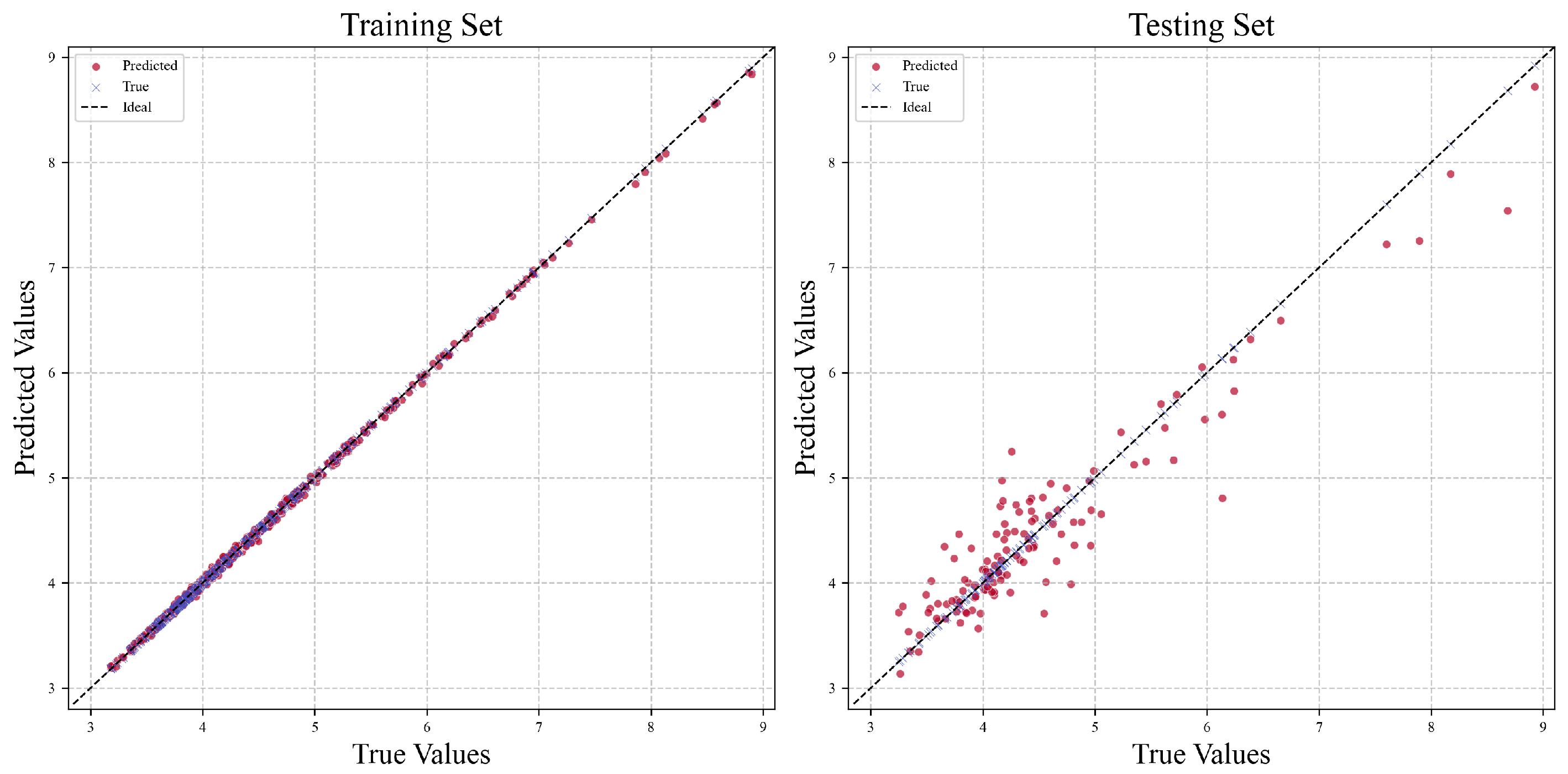
5.2. Evaluation on Surface Reconstruction Quality Estimation

To evaluate the performance of 3D reconstruction quality prediction, the CatBoost-based method is compared to multiple prevailing regression methods. As shown in

Table 3. Result comparison of different prediction models.

Model	${\mathit{R}}^2$	RMSE	MAE
SVR	0.5454	0.7032	0.4654
SVR-FE	0.5503	0.6994	0.4595
XGBoost	0.7485	0.5230	0.3612
XGBoost-FE	0.7719	0.4981	0.3474
CatBoost-FE	0.8856	0.3527	0.2466
CatBoost-LASSO	0.8606	0.3894	0.2742
CatBoost-FE-LASSO	0.8920	0.3427	0.2462

, CatBoost-FE-LASSO (prediction with feature enhancement and selection), CatBoost-FE (prediction with feature enhancement without selection), and CatBoost-LASSO (prediction with feature selection without enhancement) are compared, as well as the SVR-based [34] and XGBoost-based [35] methods.

Table 3 demonstrates that the CatBoost with feature enhancement and selection (CatBoost-FE-LASSO) proposed in this paper performs the best on all evaluation metrics. According to the results, the proposed feature enhancement is superior to feature selection in improving the CatBoost method, because CatBoost-FE outperforms CatBoost-LASSO on all metrics. However, both of them are surpassed by CatBoost-FE-LASSO, which will be employed in quality-driven planning. The advantage of the proposed feature enhancement is also demonstrated on improving the SVR and XGBoost models. Both regressions can be improved by using feature enhancement to learn the SVR-FE and XGBoost-FE models.

The scatter plots illustrating the predicted and true values are shown in Figure 6 for both training and testing sets. An ideal reference line, which represents perfect prediction, is included at a 45-degree angle. From the visualization, we can see that the data points in both training and testing sets are well-distributed, clustering closely around this ideal line. For example, most points in the test set are clustered around the ideal line, indicating that the model has a strong generalization ability. This can also interpret the advantage of CatBoost-FE-LASSO over other models based on SVR and XGBoost, 0.3427 vs. 0.6994 and 0.4981 on $RMSE$ in Table 3 for instance. Specifically, the $R^2$ value of CatBoost-FE-LASSO on the testing set is close to 0.9, reflecting that the model maintains a high prediction accuracy on unseen data. Despite the usefulness of the modeling approach in predicting the quality of reconstruction, there is still much room for further improvement by utilizing external factors such as atmospheric conditions and satellite attitude stability, etc.

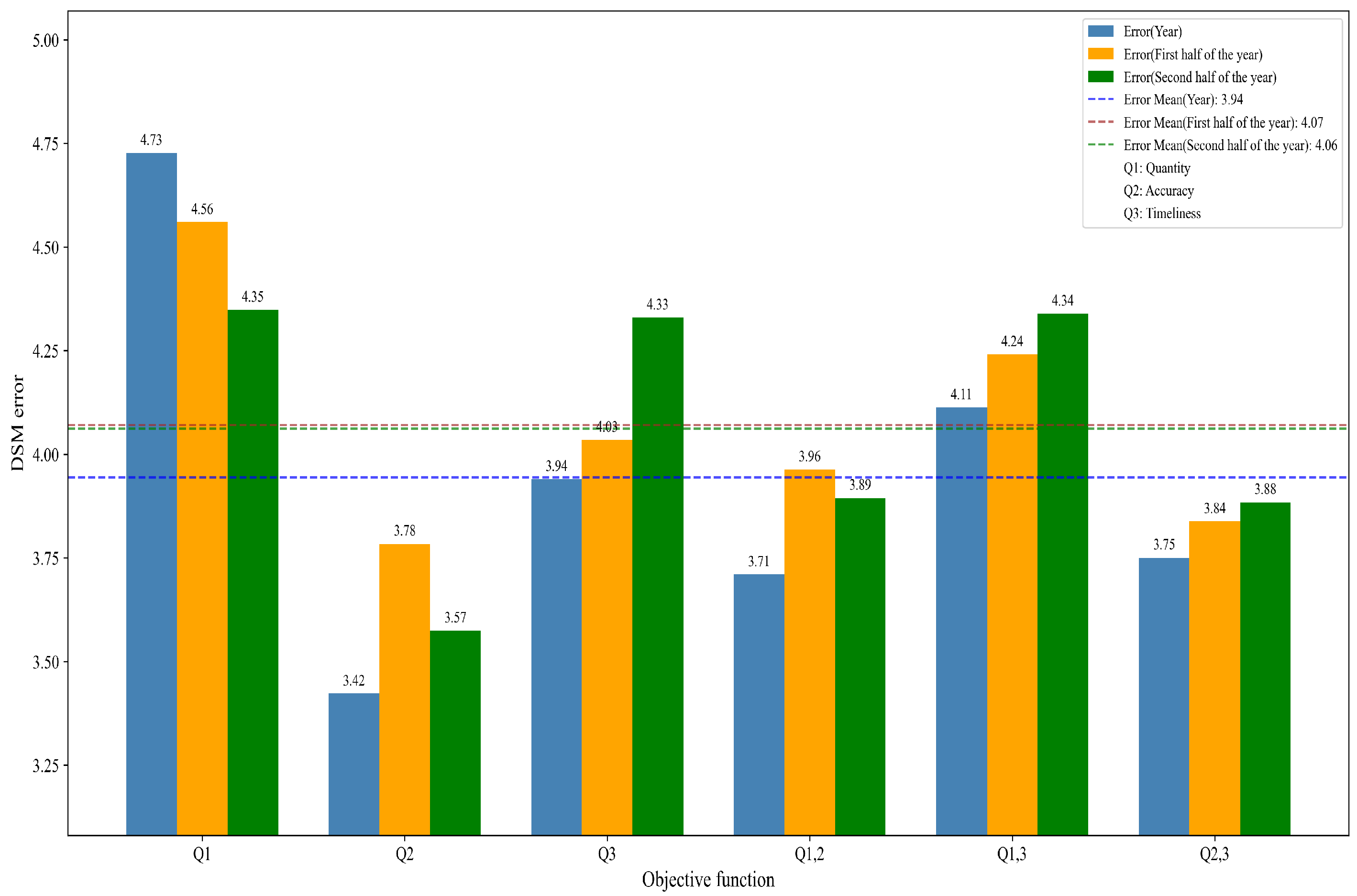
5.3. Evaluation on Planning Using Single Satellite

In this part, the planning results are evaluated using a single satellite of World-View3 as shown in Figure 5, i.e., searching from the 150 time windows localized from the World-View3 orbit as the potential imaging opportunities. This means the task planning needs to search from more than 20,000 stereo pairs to achieve optimal objective function values as modeled in Section 4.1. In solving the single-satellite planning model, the DSM quality of an arbitrary image pair is estimated beforehand using the method as proposed in Section 3.2 to quantify each possible combination. Based on this accurate quantification, the planning model is solved by the GWO algorithm whose setting of parameters is as follows: maximum number of iterations $T=500$; population size $N=100$; stereo image pair intersection angle range ${\theta }_{ij}\in [5^{\circ },{25}^{\circ }]$. The time complexity of the GWO algorithm in this scenario is $O(T·N·M^2)$, where M is the number of time windows, i.e., possible visible duration calculated according to satellite’s orbit.

To verify the effectiveness of our planning algorithm in selecting imaging opportunities to generate higher quality stereo surfaces, we compare different prioritized objective functions by controlling the objective weights in Equation (6), i.e., task quantity (${\omega }_2,{\omega }_3=0$), stereo image quality (${\omega }_1,{\omega }_3=0$), and task timeliness (${\omega }_1,{\omega }_2=0$). With these criteria, the combinations of imaging time windows are optimized to achieve the highest objective scores as is possible. In Figure 7, each averaged 3D reconstruction error is calculated over 10 independent planned results for different objectives of quantity only ($Q_1$), quality ($Q_2$), timeliness ($Q_3$), quantity and quality ($Q_{1,2}$), quantity and timeliness ($Q_{1,3}$), etc., respectively. Results of planning over a whole year (from Nov 2014 to Jan 2016) and two halves of the year 2015 are shown in Figure 7. As shown in this figure, planning with quality ($Q_2$) achieves the best performance, while planning for task quantity ($Q_1$) leads to the highest reconstruction error. While $Q_3$ lies between $Q_2$ and $Q_1$, the introduction of quality in planning can still improve the overall performance with higher $Q_{2,3}$ (${\omega }_1=0$), similar to the improved $Q_{1,2}$ (${\omega }_3=0$) compared to $Q_1$. This demonstrates the importance of quality in planning for better stereo pairs by the results of planning over both a whole year (blue) and a half year (orange or green) in Figure 7.

It is interesting to notice that the quality of stereo imaging distributes differently in the first and second halves of the year 2015. This is depicted by the difference of two halves on objectives such as $Q_2$ and $Q_3$. In Figure 7, the second half of 2015 exceeds the first half with lower DSM error (3.57 vs. 3.78) on $Q_2$ while it is outperformed by the first half on $Q_3$ (4.33 vs 4.03). This is because more high-quality stereo pairs are contained in the second half of 2015, but they are distributed in the last quarter of the year. When timeliness is used as the objective, these late stereo pairs can be hardly planned. That is why quality is poor for the second half of the year on $Q_3$ (timeliness). However, when stereo quality is to be maximized, the high-quality pairs are searched and added to the schedule, achieving better quality on $Q_2$. By considering both quality and timeliness, the proposed method can keep a balance, which is demonstrated by a smaller difference between the two halves of the year on $Q_{2,3}$ in Figure 7.

6. Discussion

6.1. Quality Comparison Using Real Images

Though Figure 7 depicts the comparison based on the estimated quality values, the realistic reconstruction quality can also be evaluated because a subset of stereo pairs have the original images observed by the World-View3 satellite as described in Section 5.1. By selecting these real images from the planned results of the scenarios as shown in Figure 7, the performance of the proposed quality-driven planning method is further evaluated.

Figure 8 demonstrates the quality statistics of real 3D reconstructions using the planned stereo pairs, averaged from the same 10 planning scenarios in Figure 7 for the whole year. The quality results of the top 10 and 30 image pairs selected by the planning algorithm are presented in Figure 8 for different optimization objectives. The trend shown in Figure 8 is consistent with that in Figure 7, which validates the effectiveness of the proposed method. For instance, among the top 10 image pairs, the reconstruction error is lowest when planning based on quality objectives. This indicates that quality-driven planning effectively identifies image pairs that yield higher reconstruction accuracy for future imaging implementation. By relaxing the selection of real image pairs to the top 30, the advantage of the quality-driven planning is still obvious though the mean error slightly increases for $Q_2$ (4.00 vs. 3.98). Moreover, by combining quality with other objectives, the overall quality can be significantly boosted ($Q_{1,2}$ vs. $Q_1$), further demonstrating the effectiveness of the proposed method.

In Figure 9, we present typical 3D reconstruction results for three objectives: task quantity ((a1)–(a3) for $Q_1$), reconstruction quality ((b1)–(b3) for $Q_2$), and timeliness ((c1)–(c3) for $Q_3$). The results are selected around the average level of DSM error in Figure 8, which is 4.0 for $Q_2$, 5.2 for $Q_1$, and 4.2 for $Q_3$ to reflect the average visual quality of DSMs. The heat values in Figure 9 indicate the elevation in each DSM. It is not hard to notice that the 3D surfaces for $Q_2$ (middle row) are much smoother than the others. Meanwhile, when optimizing for $Q_2$, surface details such as building structures can be accurately constructed, which is consistent with the lowest DSM error values illustrated in Figure 8. Though using $Q_3$ (bottom row) as an objective achieves better quality than $Q_1$, it still falls short compared to $Q_2$ in terms of both DSM error and visual appearance.

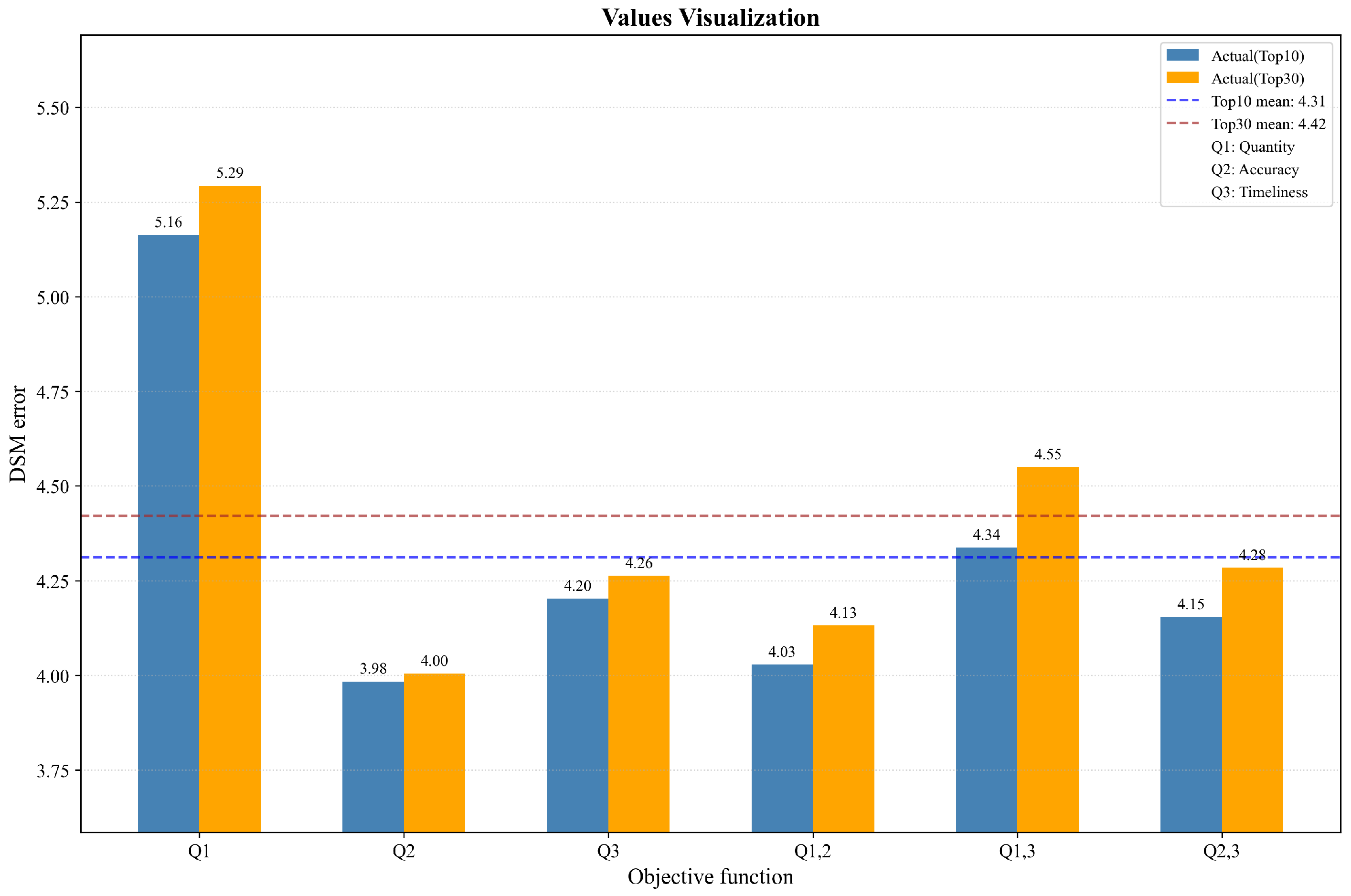
6.2. Further Planning Using Simulated Constellation

When verifying the effectiveness of the proposed planning algorithm in selecting imaging pairing opportunities to generate higher-quality stereo surface, the previous evaluation is carried out using data from a single satellite (WorldView-3). With the development of satellite constellation, multi-satellite collaborative planning has become an important means to further improve observation efficiency and data quality. Therefore, in order to further verify the performance of the algorithm in more complex and practical application scenarios, we simulated a constellation consisting of multiple satellites (including WorldView-3, WorldView-1, WorldView-2, and GeoEye-1), as shown in Figure 5, based on which more experimental evaluation is carried out in this section.

Similar to the case in Section 5.3, the imaging time windows are localized for each satellite based on its orbit. For each potential image pair, the quality of the DSM is assessed to identify stereo pairs with high reconstruction qualities in the planning algorithm. The average reconstruction quality of the selected imaging pairs is presented in Figure 10 for different objectives.

As shown in Figure 10, the quality-driven planning method still returns the best overall reconstruction performance on the quality objective ($Q_2$). This result is consistent with the single satellite result in Figure 7, for planning within the time span of both the whole year and a half of the year. Because more opportunities are available for Earth imaging using multiple satellites, the planning is more computationally complex. However, the quality-driven method can still return the searched stereo pairs in seconds, showing the promising scalability to large-scale problem settings.

7. Conclusions and Future Work

This paper addressed the challenge of satellite stereo image acquisition for high-quality 3D surface reconstruction, whose planning is not well addressed. By proposing a quality-driven planning method, this paper has demonstrated that the selection of stereo pairs can be significantly improved through a combination of regression-based quality estimation and multi-objective optimization. The proposed method leverages a CatBoost regression model with feature enhancement and selection to predict DSM quality based on various factors including intersection angle, sun elevation angle, sun azimuth angle, time intervals, etc., to enable accurate quality estimation before image acquisition. Furthermore, the quality-driven planning is modeled and solved using the Grey Wolf Optimizer and can effectively balance different requirements like task quantity, reconstruction quality, and task timeliness, ensuring efficient use of satellite resources. Experimental results on the public 3D mapping dataset and simulations validate the effectiveness of the proposed approach. Future work can be to extend the method to more flexible collaborative stereo sensing in larger constellations.

References

1. Zhang, K.; Snavely, N.; Sun, J. Leveraging vision reconstruction pipelines for satellite imagery. In Proceedings of the IEEE/CVF International Conference on Computer Vision Workshops, Seoul, Republic of Korea, 27–28 October 2019. [Google Scholar]
2. Bosch, M.; Kurtz, Z.; Hagstrom, S.; Brown, M. A multiple view stereo benchmark for satellite imagery. In Proceedings of the 2016 IEEE Applied Imagery Pattern Recognition Workshop (AIPR), Washington, DC, USA, 18–20 October 2016; pp. 1–9. [Google Scholar]
3. Beyer, R.A.; Alexandrov, O.; McMichael, S. The Ames Stereo Pipeline: NASA’s open source software for deriving and processing terrain data. Earth Space Sci. 2018, 5, 537–548. [Google Scholar] [CrossRef]
4. Wang, P.; Shi, L.; Chen, B.; Hu, Z.; Qiao, J.; Dong, Q. Pursuing 3-D scene structures with optical satellite images from affine reconstruction to Euclidean reconstruction. IEEE Trans. Geosci. Remote Sens. 2022, 60, 5632214. [Google Scholar] [CrossRef]
5. Zhao, L.; Liu, Y.; Men, C.; Men, Y. Double propagation stereo matching for urban 3-d reconstruction from satellite imagery. IEEE Trans. Geosci. Remote Sens. 2021, 60, 5601717. [Google Scholar] [CrossRef]
6. Yang, S.; Chen, H.; Chen, W. Generalized Stereo Matching Method Based on Iterative Optimization of Hierarchical Graph Structure Consistency Cost for Urban 3D Reconstruction. Remote Sens. 2023, 15, 2369. [Google Scholar] [CrossRef]
7. Orsingher, M.; Zani, P.; Medici, P.; Bertozzi, M. Revisiting PatchMatch multi-view stereo for urban 3D reconstruction. In Proceedings of the 2022 IEEE Intelligent Vehicles Symposium (IV), Aachen, Germany, 4–9 June 2022; pp. 190–196. [Google Scholar]
8. Stucker, C.; Schindler, K. ResDepth: A deep residual prior for 3D reconstruction from high-resolution satellite images. ISPRS J. Photogramm. Remote Sens. 2022, 183, 560–580. [Google Scholar] [CrossRef]
9. Oh, J.; Lee, W.H.; Toth, C.K.; Grejner-Brzezinska, D.A.; Lee, C. A Piecewise Approach to Epipolar Resampling of Pushbroom Satellite Images Based on RPC. Photogramm. Eng. Remote Sens. 2010, 76, 1353–1363. [Google Scholar] [CrossRef]
10. Carl, S.; Bärisch, S.; Lang, F.; d’Angelo, P.; Arefi, H.; Reinartz, P. Operational Generation of High-Resolution Digital Surface Models from Commercial Tri-Stereo Satellite Data. Photogramm. Week 2013, 13, 261–269. [Google Scholar]
11. D’Angelo, P.; Rossi, C.; Minet, C.; Eineder, M.; Flory, M.; Niemeyer, I. High Resolution 3D Earth Observation Data Analysis for Safeguards Activities. In Proceedings of the 12th Symposium on International Safeguards, Vienna, Austria, 20–24 0ctober 2014. [Google Scholar]
12. Qin, R. A Critical Analysis of Satellite Stereo Pairs for Digital Surface Model Generation and A Matching Quality Prediction Model. ISPRS J. Photogramm. Remote Sens. 2019, 154, 139–150. [Google Scholar] [CrossRef]
13. Facciolo, G.; Franchis, C.D.; Meinhardt-Llopis, E. Automatic 3D Reconstruction from Multi-date Satellite Images. In Proceedings of the IEEE Conference on Computer Vision and Pattern Recognition Workshops, Honolulu, HI, USA, 21–26 July 2017. [Google Scholar] [CrossRef]
14. Krauß, T.; d’Angelo, P.; Wendt, L. Cross-track satellite stereo for 3D modelling of urban areas. Eur. J. Remote Sens. 2018, 52, 89–98. [Google Scholar] [CrossRef]
15. Pan, Y.; Hui, X.; Li, J.; Zhu, X.; Xu, F.; Wang, P. A Hybrid Method for Dense Points Enclosing and Observation Planning. In Proceedings of the 2024 IEEE International Conference on Systems, Man, and Cybernetics (SMC), Kuching, Malaysia, 6–10 October 2024; pp. 4868–4874. [Google Scholar]
16. Lu, Z.; Shen, X.; Li, D.; Cheng, S.; Wang, J.; Yao, W. Super-agile satellites imaging mission planning method considering degradation of image MTF in dynamic imaging. Int. J. Appl. Earth Obs. Geoinf. 2024, 131, 103968. [Google Scholar] [CrossRef]
17. Li, L.; Chen, H.; Li, J.; Jing, N.; Emmerich, M. Preference-based Evolutionary Many-Objective Optimization for Agile Satellite Mission Planning. IEEE Access 2018, 6, 40963–40978. [Google Scholar] [CrossRef]
18. Yang, W.; Chen, Y.; He, R.; Chang, Z.; Chen, Y. The Bi-objective Active-Scan Agile Earth Observation Satellite Scheduling Problem: Modeling and Solution Approach. In Proceedings of the 2018 IEEE Congress on Evolutionary Computation (CEC), Rio de Janeiro, Brazil, 8–13 July 2018. [Google Scholar] [CrossRef]
19. Ren, L.; Ning, X.; Wang, Z. A competitive Markov decision process model and a recursive reinforcement-learning algorithm for fairness scheduling of agile satellites. Comput. Ind. Eng. 2022, 169, 108242. [Google Scholar] [CrossRef]
20. d’Angelo, P.; Reinartz, P. DSM based orientation of large stereo satellite image blocks. Int. Arch. Photogramm. Remote Sens. Spat. Inf. Sci. 2012, 39, 209–214. [Google Scholar] [CrossRef]
21. Fischler, M.A.; Bolles, R.C. Random Sample Consensus: A Paradigm for Model Fitting with Applications To Image Analysis and Automated Cartography. Commun. ACM 1981, 24, 381–395. [Google Scholar] [CrossRef]
22. Liu, C.; Yuen, J.; Torralba, A.; Sivic, J.; Freeman, W.T. SIFT Flow: Dense Correspondence across Different Scenes; Springer: Berlin/Heidelberg, Germany, 2008. [Google Scholar] [CrossRef]
23. Dial, G.; Grodecki, J. RPC replacement camera models. In Proceedings of the American Society for Photogrammetry and Remote Sensing, Baltimore, MD, USA, 7–11 March 2005; pp. 183–191. [Google Scholar]
24. Dorogush, A.V.; Ershov, V.; Gulin, A. CatBoost: Gradient boosting with categorical features support. arXiv 2018, arXiv:1810.11363. [Google Scholar] [CrossRef]
25. Muthukrishnan, R.; Rohini, R. LASSO: A feature selection technique in predictive modeling for machine learning. In Proceedings of the 2016 IEEE International Conference on Advances in Computer Applications (ICACA), Coimbatore, India, 24 October 2016. [Google Scholar] [CrossRef]
26. Benoit, K. Linear Regression Models with Logarithmic Transformations. Lond. Sch. Econ. Lond. 2011, 22, 23–36. [Google Scholar]
27. Heaton, J. An Empirical Analysis of Feature Engineering for Predictive Modeling. In Proceedings of the SoutheastCon 2016, Norfolk, VA, USA, 30 March–3 April 2016. [Google Scholar] [CrossRef]
28. Ha, T.N.; Lubo-Robles, D.; Marfurt, K.J.; Wallet, B.C. An in-depth analysis of logarithmic data transformation and per-class normalization in machine learning: Application to unsupervised classification of a turbidite system in the Canterbury Basin, New Zealand, and supervised classification of salt in the Eugene Island minibasin, Gulf of Mexico. Interpretation 2021, 9, T685–T710. [Google Scholar]
29. Cui, C.; Wang, D. High dimensional data regression using Lasso model and neural networks with random weights. Inf. Sci. 2016, 372, 505–517. [Google Scholar] [CrossRef]
30. Luo, M.; Wang, Y.; Xie, Y.; Zhou, L.; Qiao, J.; Qiu, S.; Sun, Y. Combination of Feature Selection and CatBoost for Prediction: The First Application to the Estimation of Aboveground Biomass. Forests 2021, 12, 216. [Google Scholar] [CrossRef]
31. Kartini, D.; Nugrahadi, D.T.; Farmadi, A. Hyperparameter Tuning using GridsearchCV on The Comparison of The Activation Function of The ELM Method to The Classification of Pneumonia in Toddlers. In Proceedings of the 2021 4th International Conference of Computer and Informatics Engineering (IC2IE), Depok, Indonesia, 14–15 September 2021; pp. 390–395. [Google Scholar] [CrossRef]
32. Mirjalili, S.; Mirjalili, S.M.; Lewis, A. Grey wolf optimizer. Adv. Eng. Softw. 2014, 69, 46–61. [Google Scholar] [CrossRef]
33. Jiang, T.; Zhang, C. Application of Grey Wolf Optimization for Solving Combinatorial Problems: Job Shop and Flexible Job Shop Scheduling Cases. IEEE Access 2018, 6, 26231–26240. [Google Scholar] [CrossRef]
34. Liu, Y.; Wang, L.; Gu, K. A support vector regression (SVR)-based method for dynamic load identification using heterogeneous responses under interval uncertainties. Appl. Soft Comput. 2021, 110, 107599. [Google Scholar] [CrossRef]
35. Nguyen, H.; Cao, M.T.; Tran, X.L.; Tran, T.H.; Hoang, N.D. A novel whale optimization algorithm optimized XGBoost regression for estimating bearing capacity of concrete piles. Neural Comput. Appl. 2023, 35, 3825–3852. [Google Scholar] [CrossRef]
Figure 1. Framework of quality-driven stereo planning.
Remotesensing 17 02390 g001
Figure 2. Three-dimensional surface reconstruction using satellite image pair.
Remotesensing 17 02390 g002
Figure 3. Feature correlation heatmap.
Remotesensing 17 02390 g003
Figure 4. Feature coefficients after LASSO feature selection. ( λ = 1 × 10 6 ).
Remotesensing 17 02390 g004
Figure 5. Visualization of satellite orbits and observation area. The yellow rectangle on the right side enlarges the rectangular region to be observed.
Remotesensing 17 02390 g005
Figure 6. Evaluation of quality prediction model.
Remotesensing 17 02390 g006
Figure 7. Result comparison with estimated reconstruction quality value. DSM errors as estimated by a regression model for different optimization objectives (task quantity Q 1 , reconstruction quality Q 2 , timeliness Q 3 , and the combinations) are compared.
Remotesensing 17 02390 g007
Figure 8. Result comparison with realistic reconstruction quality values. DSM errors as measured based on ground truth for different optimization objectives (task quantity Q 1 , reconstruction quality Q 2 , timeliness Q 3 , and the combinations) are compared.
Remotesensing 17 02390 g008
Figure 9. Three-dimensional reconstruction results (top to bottom: Q 1 , Q 2 and Q 3 ). The results show that the 3D reconstruction results based on quality-driven planning using Q 2 (reconstruction quality) are superior to those of the other objectives ( Q 1 and Q 3 ) in terms of DSM error and visual smoothness.
Remotesensing 17 02390 g009
Figure 10. Result comparison using simulated constellation.
Remotesensing 17 02390 g010