
A Multi-Level Semi-Automatic Procedure for the Monitoring of Bridges in Road Infrastructure Using MT-DInSAR Data


Abstract
1. Introduction
2. Proposed Methodology
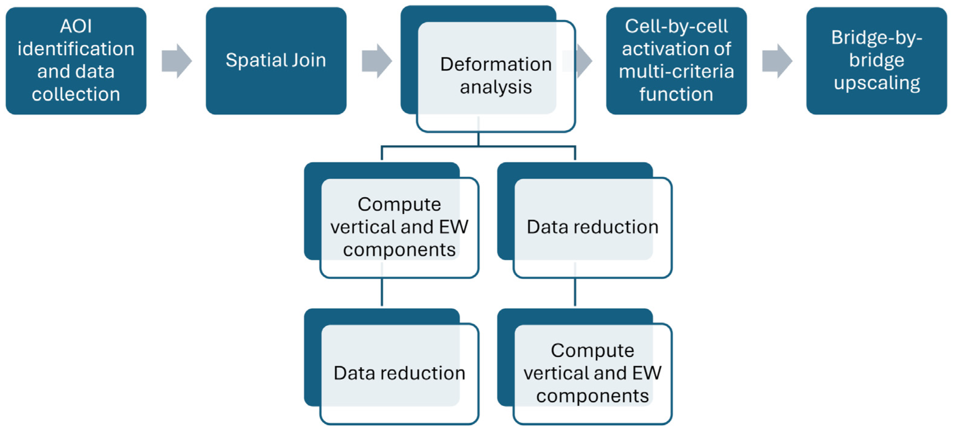
2.1. Workflow
- A satellite data dataset in the AOI.The monitoring process relies on Multi-Temporal Differential Interferometric Synthetic Aperture Radar (MT-DInSAR) analysis. Different satellite data can be adopted. Among the most commonly used datasets, the data from the Sentinel constellation processed and made available by the European Ground Motion Service (EGMS) are well-suited for broad-scale applications, while, for example, data from the first- and second-generation COSMO-SkyMed (CSK) constellations are more effective when applied to smaller, localized areas.
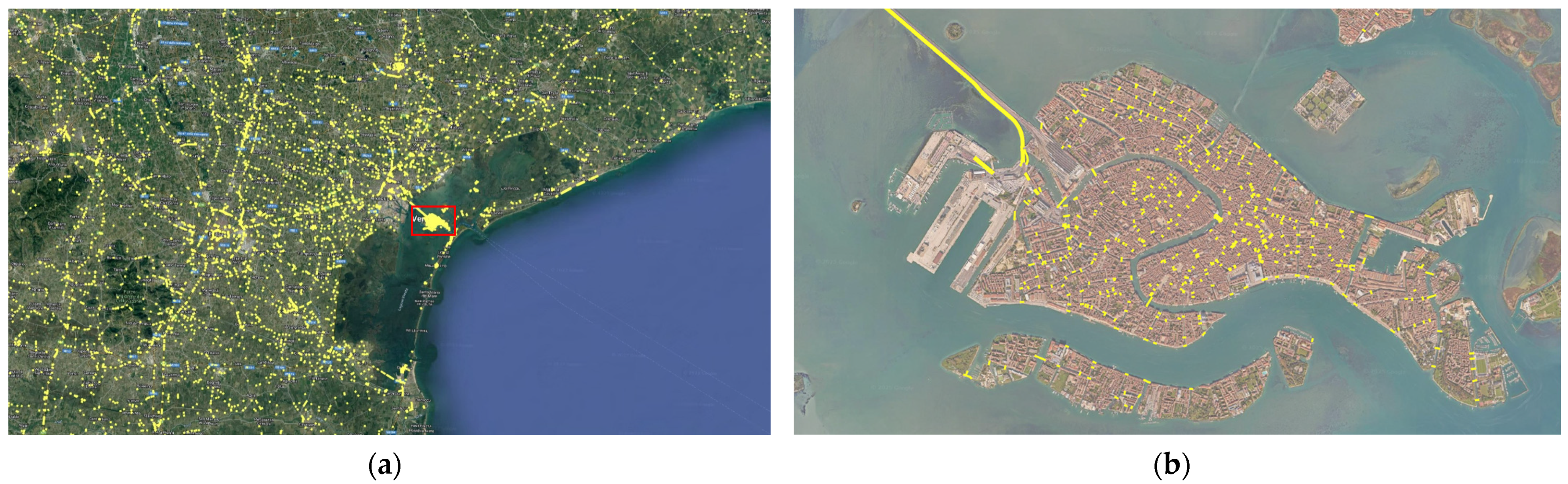
- A georeferenced database of bridges in the AOI.The proposed methodology requires the availability of polygons representing bridges in order to enable spatial queries and the filtering of measurement points (also named as PSs, Persistent Scatterers). However, existing datasets often only provide point geometries indicating bridge locations (latitude and longitude coordinates) within Geographic Information System (GIS) environments, thus requiring additional processing to determine bridge lengths and, subsequently, potential widths.
2.2. Key Datasets
2.2.1. Satellite Data
- -
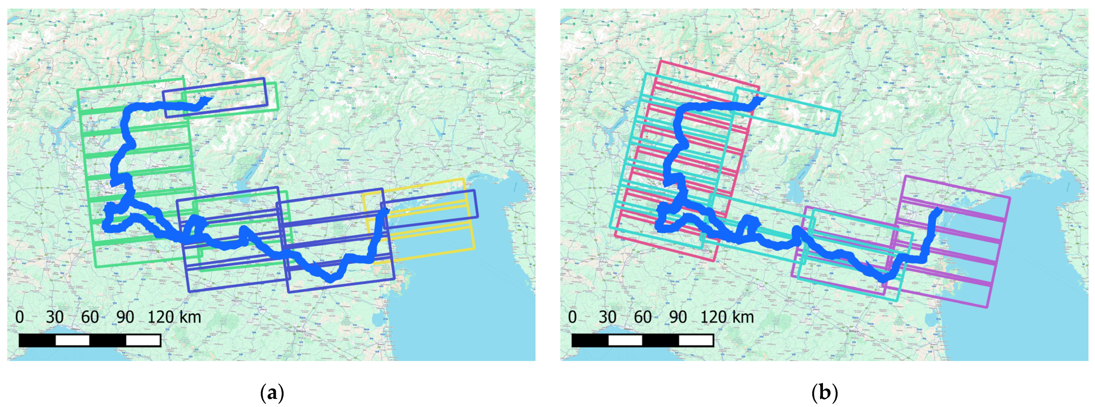
- Basic (Level 2a): This provides displacement measurements along the satellite Line of Sight (LOS) for single data tiles with respect to a local virtual reference point located within each data tile. This means that every data tile has its own reference point, making the velocities and displacement measures relative. It contains geo-localization information (both in plan and in elevation), temporal coherence, displacement velocity (both mean and standard deviation), acceleration (both mean and standard deviation) and seasonal component (both mean and standard deviation), together with the full time series of displacement for each PS. The full resolution (i.e., about 5 × 20 m) of the Sentinel sensor is exploited. The product is delivered as separate datasets for the different tracks and for both ascending and descending orbit geometries.
- -
- Calibrated (Level 2b): This provides data corrected using a GNSS-based deformation model, thereby making all the displacement measures absolute (referenced to an Earth-centered datum). This product contains the same information as the Basic one and exploits the full resolution of the Sentinel sensor of about 5 × 20 m. In this case the product is delivered as separate datasets for ascending and descending orbit geometries.
- -
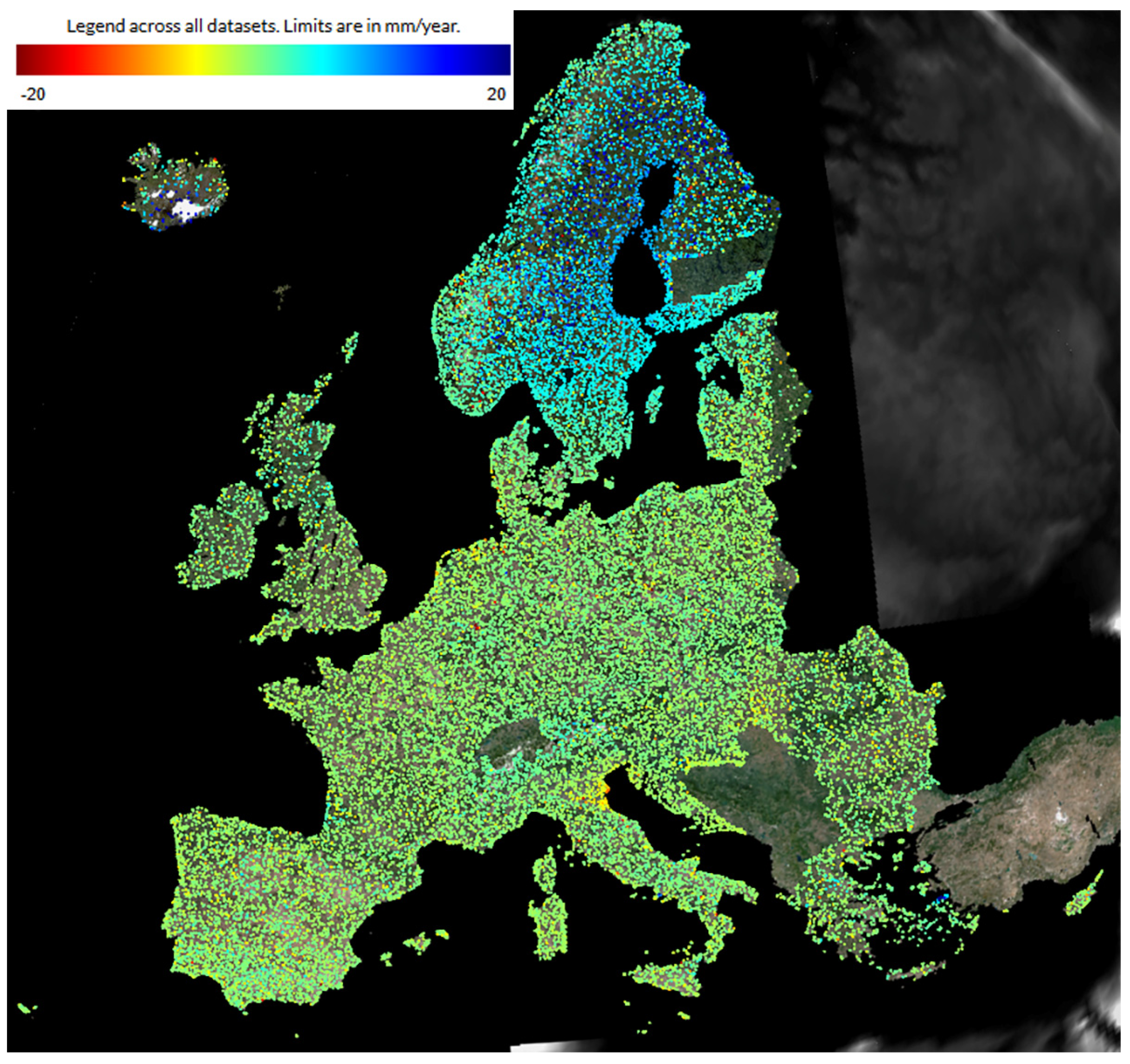
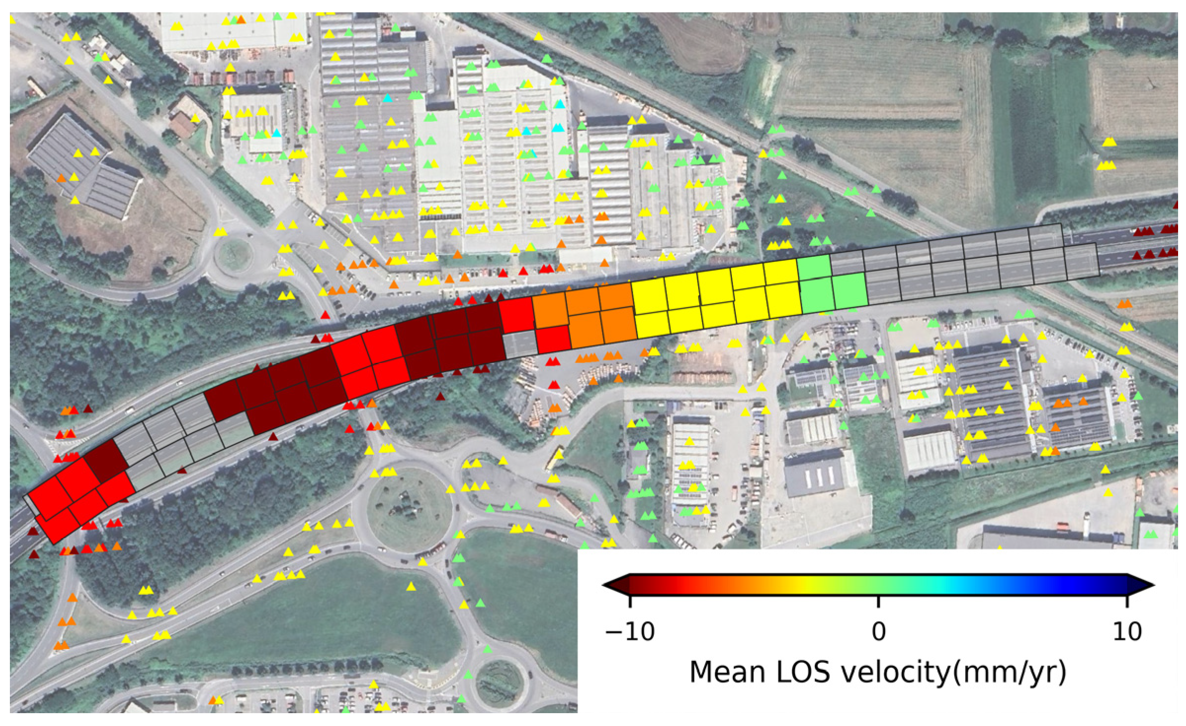
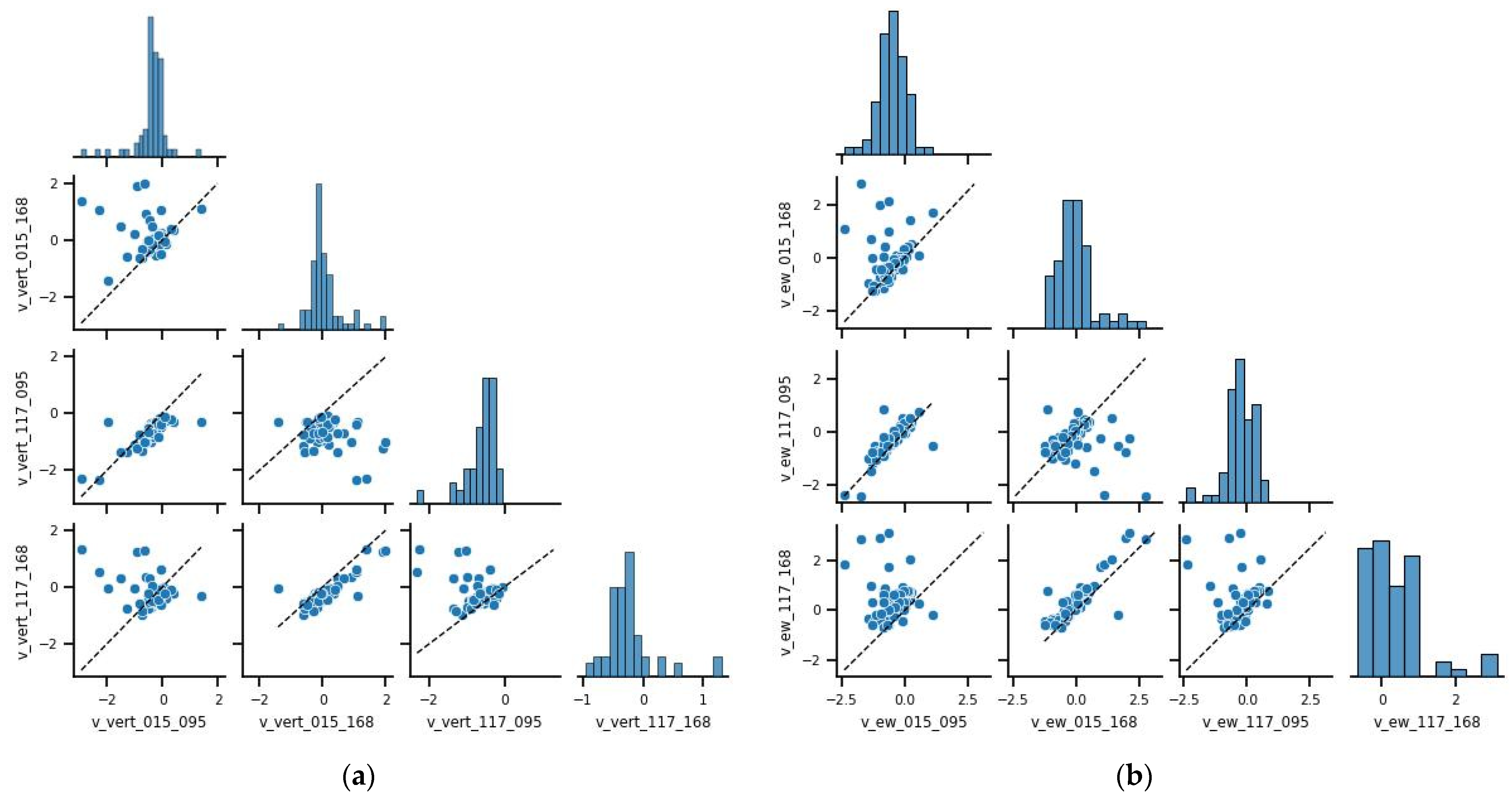
- Ortho (Level 3): Starting from ascending and descending L2b (i.e., calibrated) products, these data are combined to solve for mean vertical and horizontal east–west velocities at each location. To achieve this result, the ascending and descending L2b datasets are down-sampled to a regular 100 m × 100 m grid. The resulting L3 dataset provides the time series and velocities of ground motion in standard geographic directions, which can be easier to interpret for large-scale ground stability assessment. Ortho products are anchored to the GNSS reference frame (i.e., the measures are absolute) and are organized in 100 km × 100 km tiles for dissemination. Unfortunately, due to the poor spatial resolution, this product cannot be used generally for structural health monitoring, even at territorial scale.
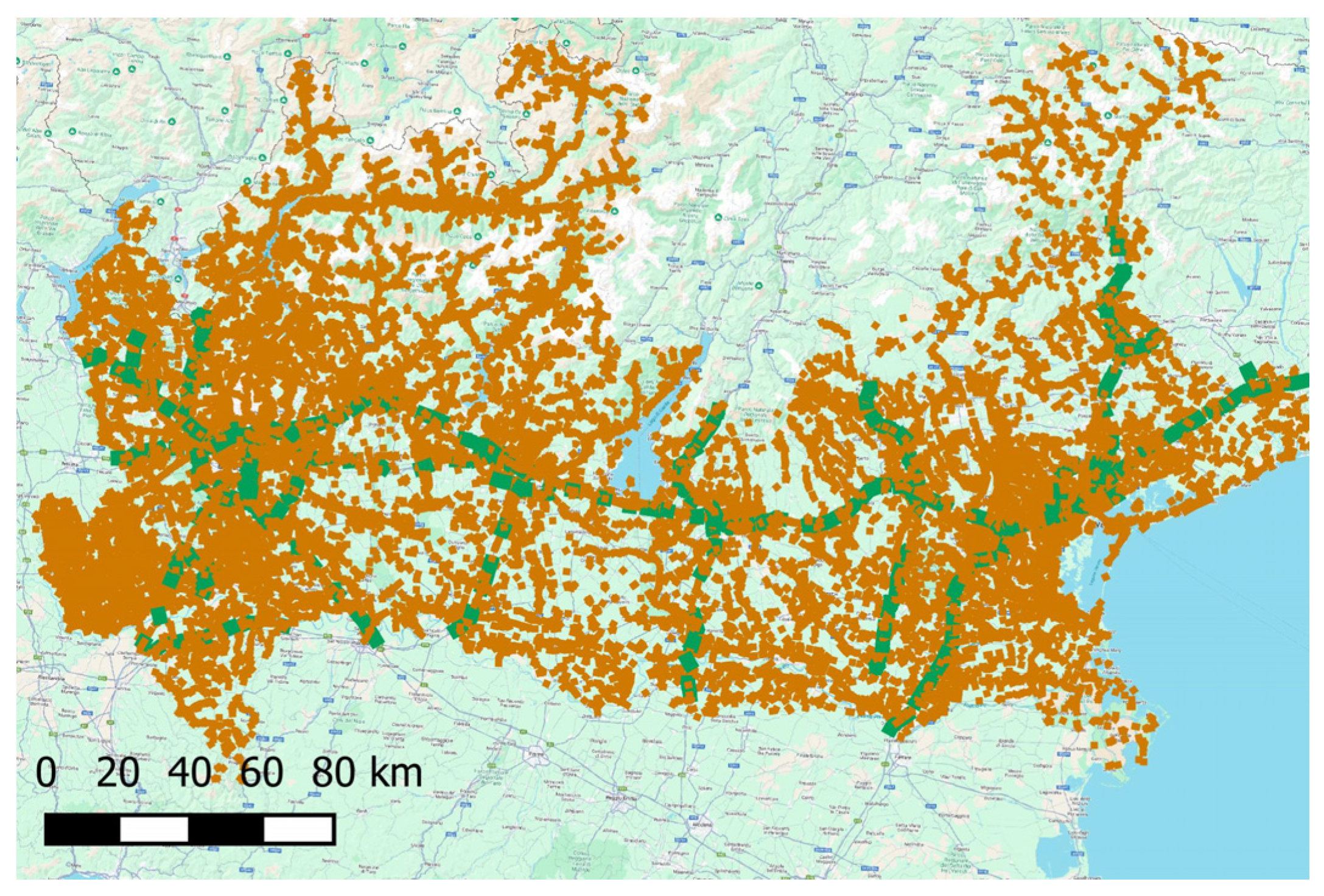
2.2.2. Bridges Dataset
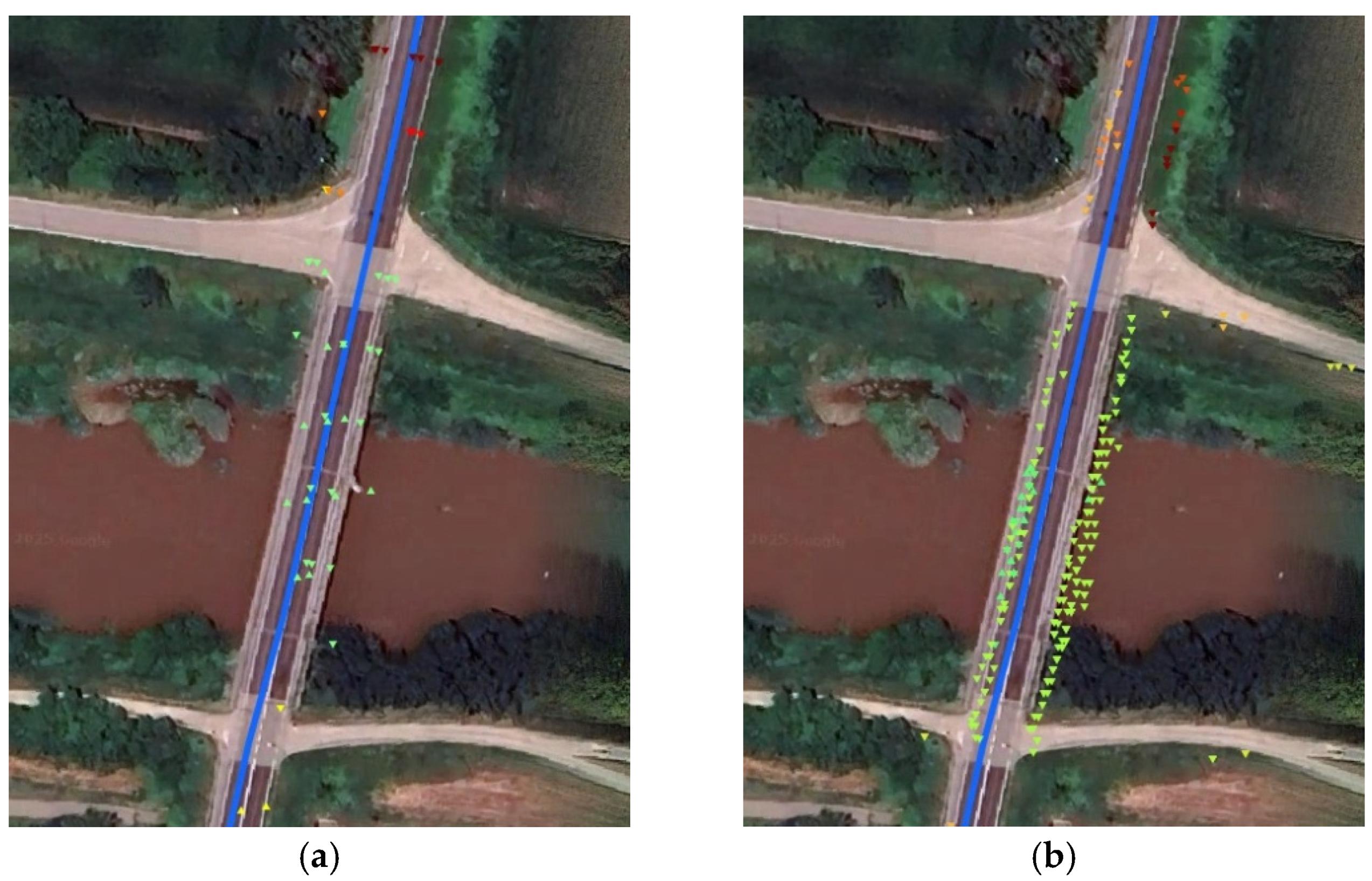
2.3. Spatial Join and Deformation Analysis
- -
- The number and density of PS points;
- -
- The mean coherence of the PS points;
- -
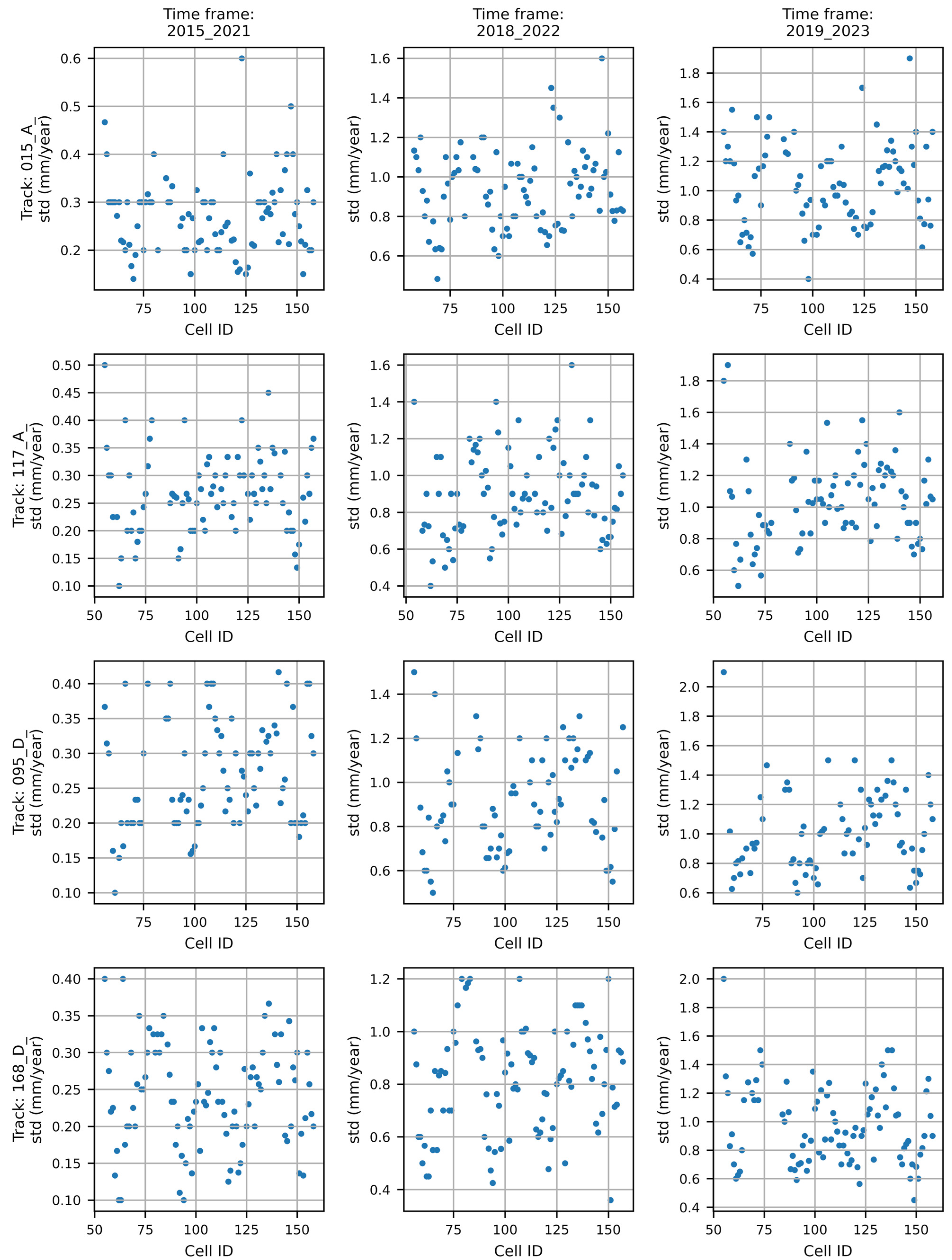
- The mean and standard deviation of the LOS velocities;
- -
- The mean time series of displacement.
2.4. Alert System and Upscaling
3. Case Study: Definition of AOI and Data Collection
4. Results
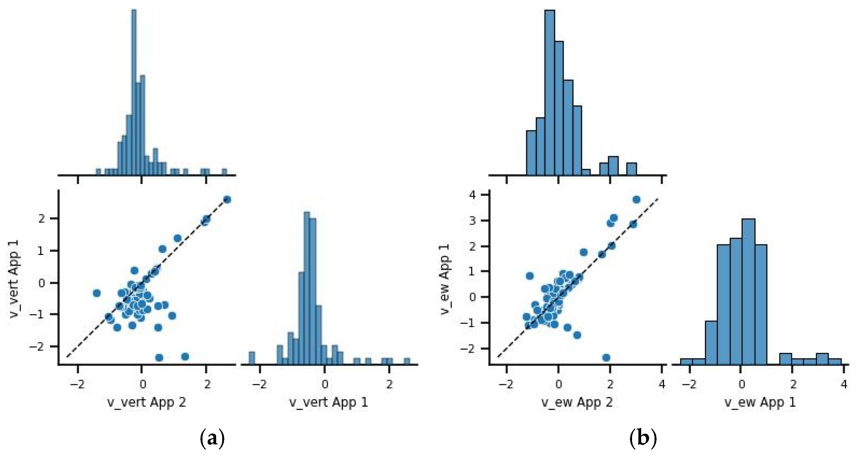
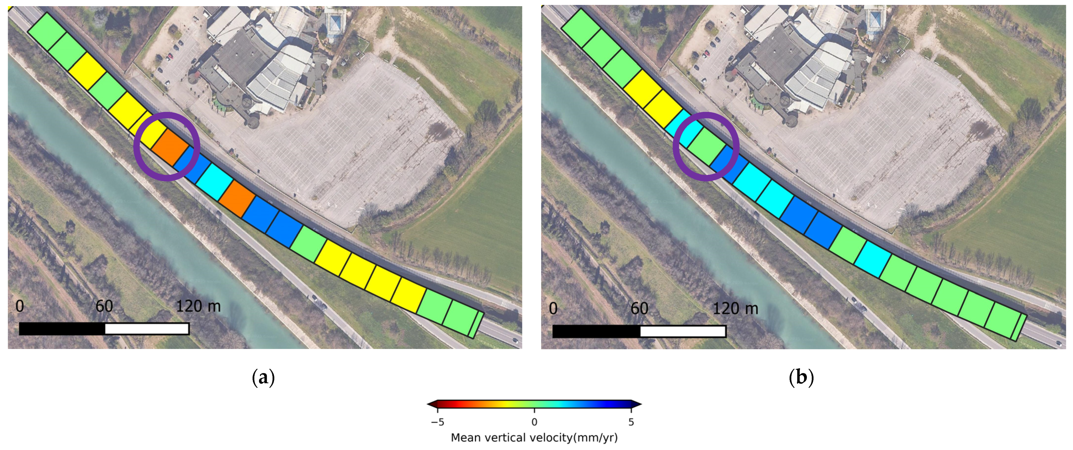
4.1. Spatial Join and Deformation Analysis
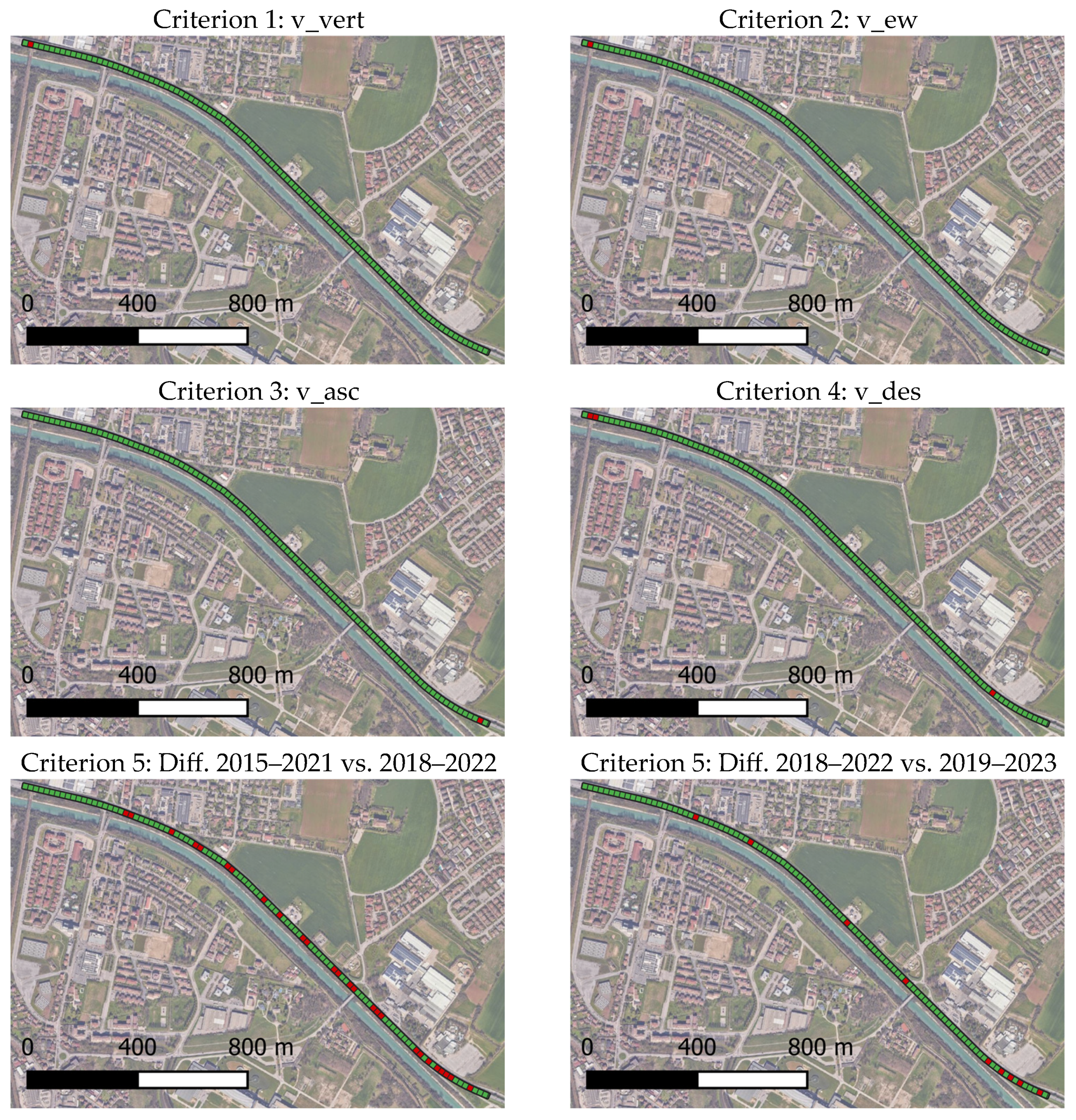
4.2. Alert System and Upscaling
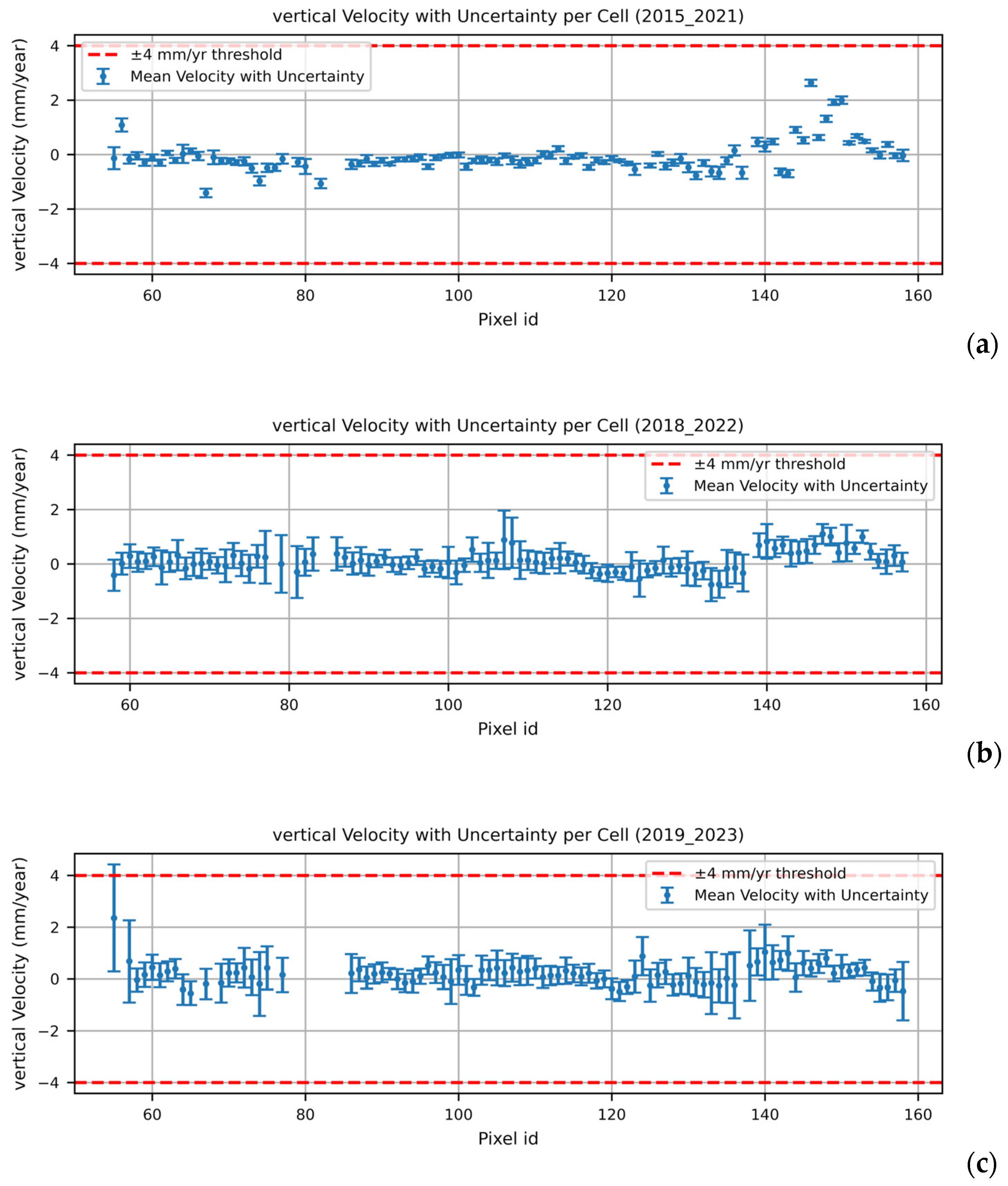
- A mean vertical velocity higher than a threshold of 4 mm/yr;
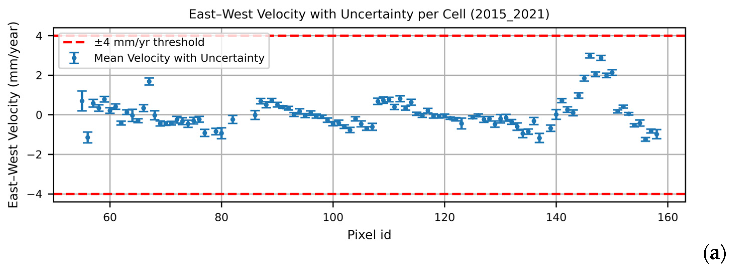
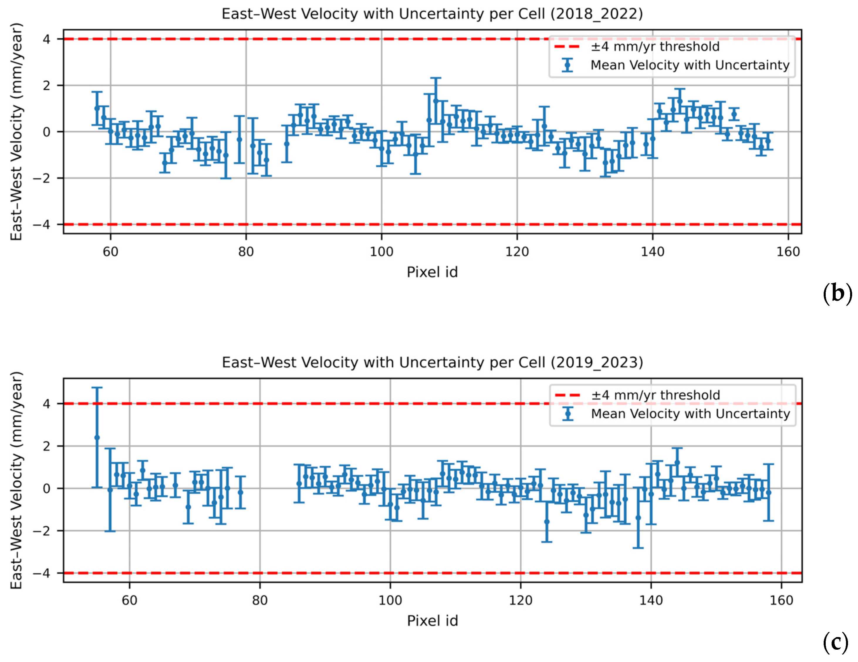
- A mean horizontal velocity higher than a threshold of 4 mm/yr;
- An ascending mean velocity along the LOS higher than a threshold of 4 mm/yr;
- A descending mean velocity along the LOS higher than a threshold of 4 mm/yr;
- Variation with respect to the previous time window larger than 100% for each of the above mentioned data points.
5. Discussion
6. Conclusions
Author Contributions
Funding
Data Availability Statement
Conflicts of Interest
References
- Ferretti, A.; Prati, C.; Rocca, F. Permanent Scatterers in SAR Interferometry. IEEE Trans. Geosci. Remote Sens. 2001, 39, 8–20. [Google Scholar] [CrossRef]
- Ferretti, A.; Fumagalli, A.; Novali, F.; Prati, C.; Rocca, F.; Rucci, A. A New Algorithm for Processing Interferometric Data-Stacks: SqueeSAR. IEEE Trans. Geosci. Remote Sens. 2011, 49, 3460–3470. [Google Scholar] [CrossRef]
- Berardino, P.; Fornaro, G.; Lanari, R.; Sansosti, E. A New Algorithm for Surface Deformation Monitoring Based on Small Baseline Differential SAR Interferograms. IEEE Trans. Geosci. Remote Sens. 2002, 40, 2375–2383. [Google Scholar] [CrossRef]
- Perissin, D.; Wang, T. Repeat-Pass SAR Interferometry with Partially Coherent Targets. IEEE Trans. Geosci. Remote Sens. 2012, 50, 271–280. [Google Scholar] [CrossRef]
- Milillo, P.; Giardina, G.; Perissin, D.; Milillo, G.; Coletta, A.; Terranova, C. Pre-Collapse Space Geodetic Observations of Critical Infrastructure: The Morandi Bridge, Genoa, Italy. Remote Sens. 2019, 11, 1403. [Google Scholar] [CrossRef]
- Infante, D.; Di Martire, D.; Calcaterra, D.; Miele, P.; Scotto di Santolo, A.; Ramondini, M. Integrated Procedure for Monitoring and Assessment of Linear Infrastructures Safety (I-Pro MONALISA) Affected by Slope Instability. Appl. Sci. 2019, 9, 5535. [Google Scholar] [CrossRef]
- Tonelli, D.; Caspani, V.F.; Valentini, A.; Rocca, A.; Torboli, R.; Vitti, A.; Perissin, D.; Zonta, D. Interpretation of Bridge Health Monitoring Data from Satellite InSAR Technology. Remote Sens. 2023, 15, 5242. [Google Scholar] [CrossRef]
- Chang, L.; Dollevoet, R.P.B.J.; Hanssen, R.F. Nationwide Railway Monitoring Using Satellite SAR Interferometry. IEEE J. Sel. Top. Appl. Earth Obs. Remote Sens. 2017, 10, 596–604. [Google Scholar] [CrossRef]
- Macchiarulo, V.; Milillo, P.; Blenkinsopp, C.; Giardina, G. Monitoring Deformations of Infrastructure Networks: A Fully Automated GIS Integration and Analysis of InSAR Time-Series. Struct. Health Monit. 2022, 21, 1849–1878. [Google Scholar] [CrossRef]
- Selvakumaran, S.; Plank, S.; Geiß, C.; Rossi, C.; Middleton, C. Remote Monitoring to Predict Bridge Scour Failure Using Interferometric Synthetic Aperture Radar (InSAR) Stacking Techniques. Int. J. Appl. Earth Obs. Geoinf. 2018, 73, 463–470. [Google Scholar] [CrossRef]
- Cusson, D.; Rossi, C.; Ozkan, I.F. Early Warning System for the Detection of Unexpected Bridge Displacements from Radar Satellite Data. J. Civ. Struct. Health Monit. 2021, 11, 189–204. [Google Scholar] [CrossRef]
- Cusson, D.; Trischuk, K.; Hébert, D.; Hewus, G.; Gara, M.; Ghuman, P. Satellite-Based InSAR Monitoring of Highway Bridges: Validation Case Study on the North Channel Bridge in Ontario, Canada. Transp. Res. Rec. J. Transp. Res. Board. 2018, 2672, 76–86. [Google Scholar] [CrossRef]
- Talledo, D.A.; Miano, A.; Bonano, M.; Di Carlo, F.; Lanari, R.; Manunta, M.; Meda, A.; Mele, A.; Prota, A.; Saetta, A.; et al. Satellite Radar Interferometry: Potential and Limitations for Structural Assessment and Monitoring. J. Build. Eng. 2022, 46, 103756. [Google Scholar] [CrossRef]
- Jung, J.; Kim, D.; Palanisamy Vadivel, S.K.; Yun, S.-H. Long-Term Deflection Monitoring for Bridges Using X and C-Band Time-Series SAR Interferometry. Remote Sens. 2019, 11, 1258. [Google Scholar] [CrossRef]
- Lazecky, M.; Hlavacova, I.; Bakon, M.; Sousa, J.J.; Perissin, D.; Patricio, G. Bridge Displacements Monitoring Using Space-Borne X-Band SAR Interferometry. IEEE J. Sel. Top. Appl. Earth Obs. Remote Sens. 2017, 10, 205–210. [Google Scholar] [CrossRef]
- Markogiannaki, O.; Xu, H.; Chen, F.; Mitoulis, S.A.; Parcharidis, I. Monitoring of a Landmark Bridge Using SAR Interferometry Coupled with Engineering Data and Forensics. Int. J. Remote Sens. 2022, 43, 95–119. [Google Scholar] [CrossRef]
- Farneti, E.; Cavalagli, N.; Costantini, M.; Trillo, F.; Minati, F.; Venanzi, I.; Ubertini, F. A Method for Structural Monitoring of Multispan Bridges Using Satellite InSAR Data with Uncertainty Quantification and its Pre-Collapse Application to the Albiano-Magra Bridge in Italy. Struct. Health Monit. 2023, 22, 353–371. [Google Scholar] [CrossRef]
- Miano, A.; Mele, A.; Silla, M.; Bonano, M.; Striano, P.; Lanari, R.; Di Ludovico, M.; Prota, A. Space-Borne DInSAR Measurements Exploitation for Risk Classification of Bridge Networks. J. Civ. Struct. Health Monit. 2024, 15, 731–744. [Google Scholar] [CrossRef]
- Ignatenko, V.; Laurila, P.; Radius, A.; Lamentowski, L.; Antropov, O.; Muff, D. ICEYE Microsatellite SAR Constellation Status Update: Evaluation of First Commercial Imaging Modes. In Proceedings of the 2020 IEEE International Geoscience and Remote Sensing Symposium, Waikoloa, HI, USA, 26 September–2 October 2020; pp. 3581–3584. [Google Scholar] [CrossRef]
- Stringham, C.; Farquharson, G.; Castelletti, D.; Quist, E.; Riggi, L.; Eddy, D.; Soenen, S. The Capella X-Band SAR Constellation for Rapid Imaging. In Proceedings of the IGARSS 2019—2019 IEEE International Geoscience and Remote Sensing Symposium, Yokohama, Japan, 28 July–2 August 2019; pp. 9248–9251. [Google Scholar] [CrossRef]
- Macchiarulo, V.; Milillo, P.; Blenkinsopp, C.; Reale, C.; Giardina, G. Multi-Temporal InSAR for Transport Infrastructure Monitoring: Recent Trends and Challenges. Proc. Inst. Civ. Eng. Bridge Eng. 2023, 176, 92–117. [Google Scholar] [CrossRef]
- Manconi, A.; Bühler, Y.; Stoffel, A.; Gaume, J.; Zhang, Q.; Tolpekin, V. Brief Communication: Monitoring Impending Slope Failure with Very High-Resolution Spaceborne Synthetic Aperture Radar. Nat. Hazards Earth Syst. Sci. 2024, 24, 3833–3839. [Google Scholar] [CrossRef]
- Castelletti, D.; Farquharson, G.; Brown, J.; De, S.; Yague-Martinez, N.; Stringham, C.; Yalla, G.; Villarreal, A. Capella Space VHR SAR Constellation: Advanced Tasking Patterns and Future Capabilities. In Proceedings of the IGARSS 2022—2022 IEEE International Geoscience and Remote Sensing Symposium, Kuala Lumpur, Malaysia, 17–22 July 2022; pp. 4137–4140. [Google Scholar] [CrossRef]
- Banic, M.; Ristic-Durrant, D.; Madic, M.; Klapper, A.; Trifunovic, M.; Simonovic, M.; Fischer, S. The Use of Earth Observation Data for Railway Infrastructure Monitoring—A Review. Infrastructures 2025, 10, 66. [Google Scholar] [CrossRef]
- Wang, J.; Lu, Z.; Bekaert, D.; Marshak, C.; Govorcin, M.; Sangha, S.; Kennedy, J.; Gregg, P. Along-Arc Volcanism in the Western and Central Aleutian from 2015 to 2021 Revealed by Cloud-Based InSAR Processing. Geophys. Res. Lett. 2023, 50, e2023GL106323. [Google Scholar] [CrossRef]
- Talledo, D.A.; Miano, A.; Di Carlo, F.; Bonano, M.; Mele, A.; Stella, A.; Lanari, R.; Meda, A.; Prota, A.; Saetta, A. Algorithms for Large-Scale Quasi-Real Time Monitoring of Architectural and Cultural Heritage Based on MT-DInSAR Data. Lect. Notes Civ. Eng. 2023, 432, 727–735. [Google Scholar] [CrossRef]
- Abbozzo, A.; Zani, G.; Di Prisco, M. A New Approach to Improve Safe Exceptional Transpor-Tation: A Proof of Concept in the Framework of NRRP. In Proceedings of the 15th fib International PhD Symposium in Civil Engineering 2024, Budapest, Hungary, 28–30 August 2024; p. 457464. [Google Scholar]
- Costantini, M.; Minati, F.; Trillo, F.; Ferretti, A.; Novali, F.; Passera, E.; Dehls, J.; Larsen, Y.; Marinkovic, P.; Eineder, M.; et al. European Ground Motion Service (EGMS). In Proceedings of the 2021 IEEE International Geoscience and Remote Sensing Symposium, Brussels, Belgium, 11–16 July 2021; pp. 3293–3296. [Google Scholar] [CrossRef]
- Crosetto, M.; Solari, L.; Balasis-Levinsen, J.; Bateson, L.; Casagli, N.; Frei, M.; Oyen, A.; Moldestad, D.A.; Mróz, M. Deformation Monitoring at European Scale: The Copernicus Ground Motion Service. Int. Arch. Photogramm. Remote Sens. Spat. Inf. Sci. 2021, XLIII-B3-2021, 141–146. [Google Scholar] [CrossRef]
- Crosetto, M.; Solari, L.; Mróz, M.; Balasis-Levinsen, J.; Casagli, N.; Frei, M.; Oyen, A.; Moldestad, D.A.; Bateson, L.; Guerrieri, L.; et al. The Evolution of Wide-Area DInSAR: From Regional and National Services to the European Ground Motion Service. Remote Sens. 2020, 12, 2043. [Google Scholar] [CrossRef]
- Copernicus Webinar “How to Use EGMS Data”. Questions and Answers, 13 May 2024. Available online: https://land.copernicus.eu/en/events/learn-to-use-and-interpret-the-european-ground-motion-service-data/q-a_egms_webinar_responses_130524.pdf/@@download/file (accessed on 7 April 2025).
- Hrysiewicz, A.; Khoshlahjeh Azar, M.; Holohan, E.P. EGMS-Toolkit: A Set of Python Scripts for Improved Access to Datasets from the European Ground Motion Service. Earth Sci. Inf. 2024, 17, 3825–3837. [Google Scholar] [CrossRef]
- Rouault, E.; Warmerdam, F.; Schwehr, K.; Kiselev, A.; Butler, H.; Łoskot, M.; Szekeres, T.; Tourigny, E.; Landa, M.; Miara, I.; et al. GDAL. Available online: https://gdal.org/en/stable/ (accessed on 10 May 2025).
- OpenDataSicilia Github Repository to Maps of Bridges in Italy by Region. Available online: https://github.com/SiciliaHub/mappe/tree/gh-pages/pontieviadotti (accessed on 7 May 2025).
- Bevington, P.R.; Robinson, D.K. Data Reduction and Error Analysis for the Physical Sciences, 3rd ed.; McGraw-Hill Publishing: New York, NY, USA, 2003; ISBN 0072472278. [Google Scholar]
- Fuhrmann, T.; Garthwaite, M.C. Resolving Three-Dimensional Surface Motion with InSAR: Constraints from Multi-Geometry Data Fusion. Remote Sens. 2019, 11, 241. [Google Scholar] [CrossRef]
- Vradi, A.; Sala, J.; Solari, L.; Balasis-Levinsen, J. Validating the European Ground Motion Service: An Assessment of Measurement Point Density. Int. Arch. Photogramm. Remote Sens. Spat. Inf. Sci. 2023, XLVIII-4/W7-2023, 247–252. [Google Scholar] [CrossRef]
- Koudogbo, F.; Vöge, M.; Martins, J.E.; Raucoules, D.; De Michelle, M.; Vecchiotti, F. EGMS Validation Report: Third Update; EEA: Copenhagen, Denmark, 2025. [Google Scholar]


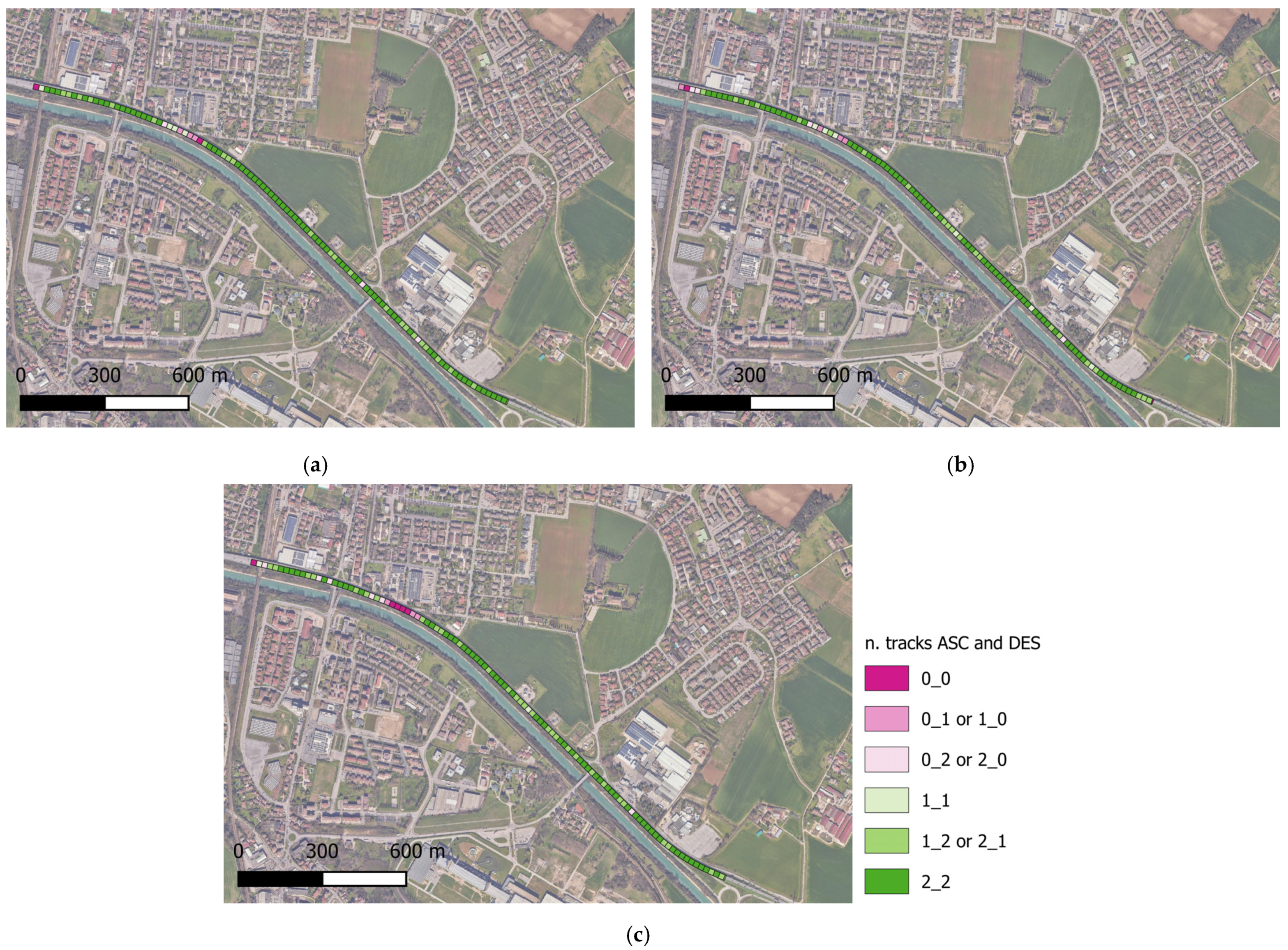
| Number of ASC, DES Tracks | Number of Possible Combinations | Number of Pixels |
|---|---|---|
| 0, 0 | 0 | 342 (11.4%) |
| 1, 0 or 0, 1 | 0 | 455 (15.2%) |
| 2, 0 or 0,2 | 0 | 333 (11.1%) |
| 1, 1 | 1 | 493 (16.4%) |
| 1, 2 or 2, 1 | 2 | 1245 (41.5%) |
| 2, 2 | 4 | 131 (4.4%) |
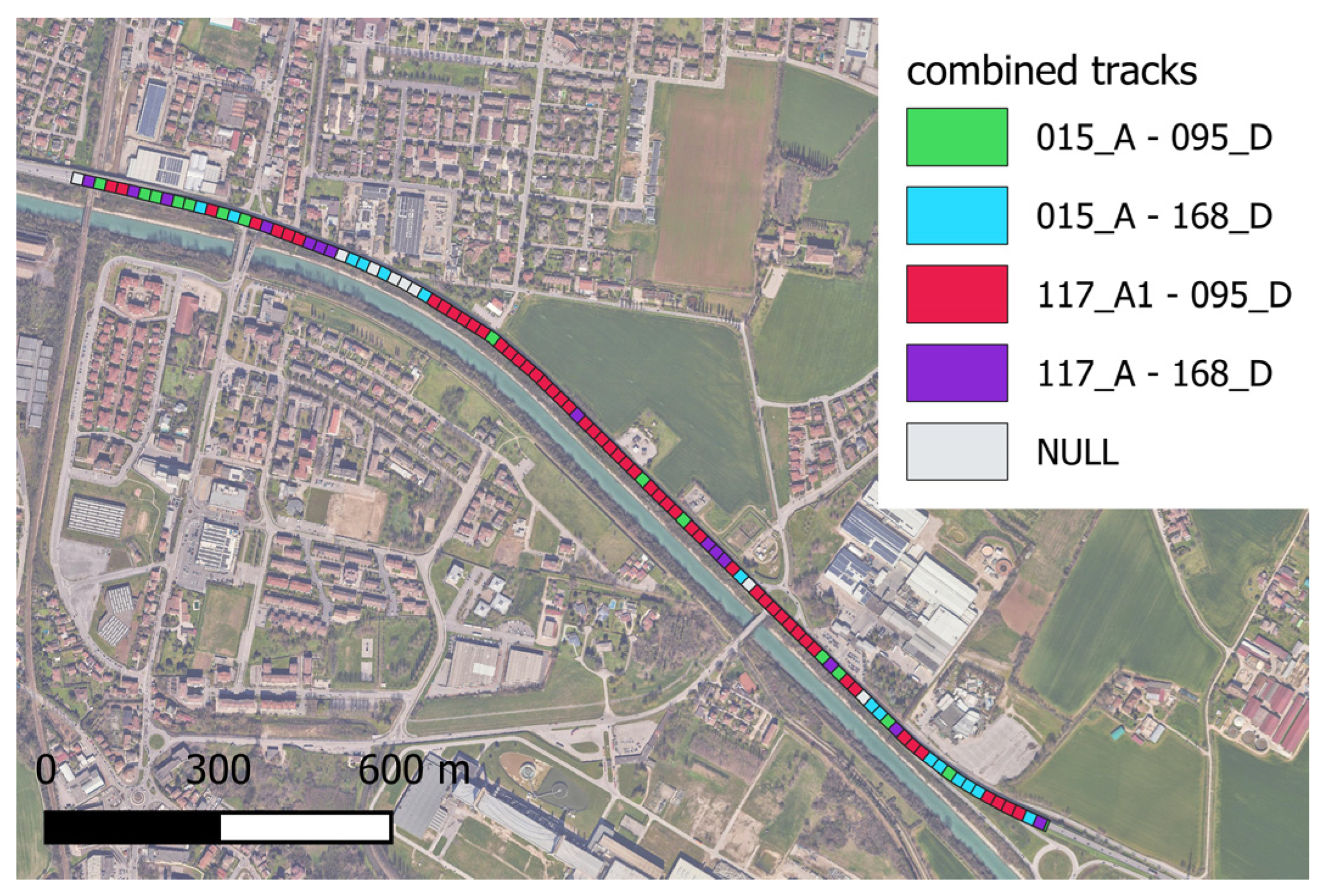
| Track and Orbit Combination | Number of Pixels |
|---|---|
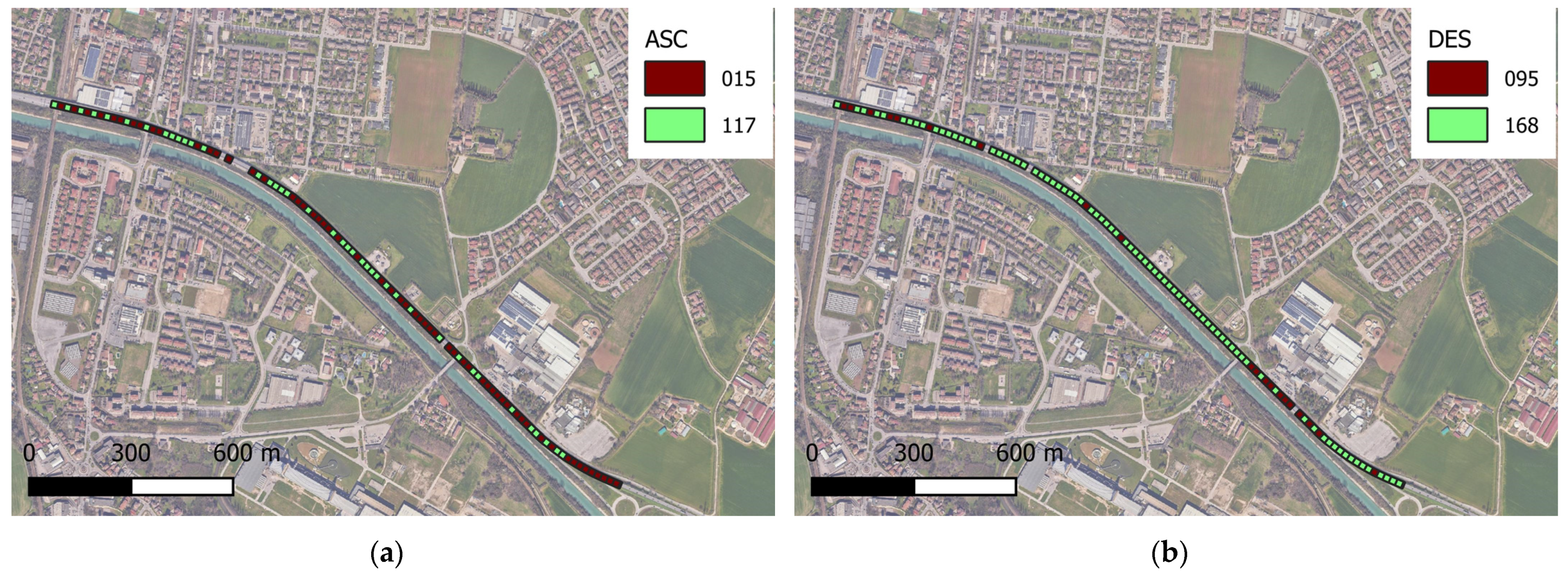
| 015 (A) | 59 |
| 117 (A) | 40 |
| 095 (D) | 21 |
| 168 (D) | 80 |
Disclaimer/Publisher’s Note: The statements, opinions and data contained in all publications are solely those of the individual author(s) and contributor(s) and not of MDPI and/or the editor(s). MDPI and/or the editor(s) disclaim responsibility for any injury to people or property resulting from any ideas, methods, instructions or products referred to in the content. |
© 2025 by the authors. Licensee MDPI, Basel, Switzerland. This article is an open access article distributed under the terms and conditions of the Creative Commons Attribution (CC BY) license (https://creativecommons.org/licenses/by/4.0/).
Share and Cite
Talledo, D.A.; Saetta, A. A Multi-Level Semi-Automatic Procedure for the Monitoring of Bridges in Road Infrastructure Using MT-DInSAR Data. Remote Sens. 2025, 17, 2377. https://doi.org/10.3390/rs17142377
Talledo DA, Saetta A. A Multi-Level Semi-Automatic Procedure for the Monitoring of Bridges in Road Infrastructure Using MT-DInSAR Data. Remote Sensing. 2025; 17(14):2377. https://doi.org/10.3390/rs17142377
Chicago/Turabian StyleTalledo, Diego Alejandro, and Anna Saetta. 2025. "A Multi-Level Semi-Automatic Procedure for the Monitoring of Bridges in Road Infrastructure Using MT-DInSAR Data" Remote Sensing 17, no. 14: 2377. https://doi.org/10.3390/rs17142377
APA StyleTalledo, D. A., & Saetta, A. (2025). A Multi-Level Semi-Automatic Procedure for the Monitoring of Bridges in Road Infrastructure Using MT-DInSAR Data. Remote Sensing, 17(14), 2377. https://doi.org/10.3390/rs17142377