Applying Deep Learning Methods for a Large-Scale Riparian Vegetation Classification from High-Resolution Multimodal Aerial Remote Sensing Data

Abstract

The unique vegetation in riparian zones is fundamental for various ecological and socio-economic functions in these transitional areas. Sustainable management requires detailed spatial information about the occurring flora. Here, we present a Deep Learning (DL)-based approach for processing multimodal high-resolution remote sensing data (aerial RGB and near-infrared (NIR) images and elevation maps) to generate a classification map of the tidal Elbe and a section of the Rhine River (Germany). The ground truth was based on existing mappings of vegetation and biotope types. The results showed that (I) despite a large class imbalance, for the tidal Elbe, a high mean Intersection over Union (IoU) of about 78% was reached. (II) At the Rhine River, a lower mean IoU was reached due to the limited amount of training data and labelling errors. Applying transfer learning methods and labelling error correction increased the mean IoU to about 60%. (III) Early fusion of the modalities was beneficial. (IV) The performance benefits from using elevation maps and the NIR channel in addition to RGB images. (V) Model uncertainty was successfully calibrated by using temperature scaling. The generalization ability of the trained model can be improved by adding more data from future aerial surveys.

1. Introduction

Riparian ecosystems are ecologically important transitional zones between land and water that play a vital role in maintaining biodiversity, water quality and habitat connectivity [1,2]. The vegetation in these areas is highly specialized and contributes to essential functions such as bank stabilization, flood protection and nutrient cycling [3]. At the same time, riparian zones are subject to intensive human use, particularly in regions where rivers serve multiple purposes. In Germany, federal waterways are an example of this duality, acting as ecologically valuable corridors while also serving as economically important transport routes. Ensuring ecological integrity while meeting economic and infrastructural demands is a key challenge in the sustainable management of riparian areas. Knowledge of the distribution of vegetation is required to meet this challenge.

Traditional methods of monitoring vegetation cover (e.g., field surveys) have several disadvantages, including being time-consuming and having limited spatial and temporal extent. Remote sensing data offer the potential for a spatially highly resolved, large-scale and frequent observation of vegetation [4]. Due to these advantages, remote sensing is nowadays a key instrument for the monitoring of ecosystems [5]. However, processing remote sensing data is still challenging because of, e.g., the large volume of data in multiple resolutions (temporal, spatial, spectral), the availability of different modalities (like optical images or elevation information) and complex image compositions [6,7,8].

Machine learning (ML) algorithms have the potential to deal with this complexity and to achieve high accuracy for a variety of tasks [9,10,11,12,13]. With recent advances in computational power and in computer vision, as well as remote sensing, Deep Learning (DL, a sub-field of ML) methods achieved remarkable performance in various applications [6,14,15]. In contrast to traditional ML, DL offers key advantages like the ability to autonomously extract features from data (reducing the need for manual data processing) and handling large amounts of data [14]. Consequently, DL methods are also frequently studied for the analysis of remote sensing data, where many studies demonstrated the benefits compared to traditional ML methods [16,17,18,19]. Furthermore, DL shows promising results for the classification of vegetation in remote sensing data [8,20,21,22,23,24,25,26,27,28,29,30,31,32,33,34]. However, it is important to note that DL is not always superior to traditional ML algorithms. Depending on the training data and task, classic ML approaches might perform better than DL (e.g., [35]).

Currently, two main types of DL architectures prevail in the semantic segmentation task in remote sensing data: convolutional neural networks (CNNs) and transformers [36]. Transformers only emerged in recent years, and thus there are few studies applying these architectures to remote sensing data. Self-attention is the main mechanism of transformers and allows capturing contexts over a long range [37]. On the other hand, CNNs are widely used and extensively studied. Thus, many CNN architectures (and modifications) were tested for the application to remote sensing data, and pre-trained models are available for use. Furthermore, CNNs capture local dependencies and are robust to small changes in an image. Compared to transformers, CNNs are computationally more efficient and usually require less training data [37,38,39]. CNNs and transformers both achieved high performance with remote sensing data [20,28,34,37,40]. There are also hybrid architectures that aim to combine the benefits of CNNs and transformers [38].

DL for classification tasks is usually applied in a supervised manner (i.e., ground truth data are used for training) when labeled data are available in a sufficient amount [6,41]. In this case, the quality of the ground truth is critical for the model performance [42]. If only limited labeled data are available, there are many approaches for training DL architectures with a low amount of labeled data or even unlabeled data (e.g., self-supervised learning) [43,44,45,46].

In contrast to images used in common computer vision applications, remote sensing data are often composed of more than three channels. Examples include multi- or hyperspectral images and additional data from other sources like elevation models. Studies showed that DL and ML methods generally benefit from high-resolution inputs [18,27] and that a combination of data from different sources is usually beneficial for the performance of DL models [8,47,48,49,50]. However, there are many options for combining different modalities. These can be broadly categorized into early and late fusion approaches [51]. In the early fusion approaches, the data from each source are combined in early stages of the models. A simple example is the concatenation of the data from each modality, which is then jointly used as an input for a model. Early fusion approaches are usually simpler to implement, and the number of trainable parameters in the model is only slightly increased. The data must be aligned to be suitable for the joint processing [51,52]. Late fusion methods fuse the data at a later step in a network. Often, each modality is processed by a separate model, and the extracted features are fused before the prediction of the model. Alternatively, each separate model can produce a prediction, and the predictions are averaged to obtain the final result. Thus, late fusion models heavily increase the number of trainable parameters, but are also powerful, since each modality is processed by a specialized model [52]. There are also middle fusion approaches, where the modalities (or the extracted features) are fused in the middle of the model [53,54]. Besides providing different modalities as inputs, DL and ML methods also generally benefit from high-resolution inputs.

In this study, we propose a DL-based workflow for classifying riparian vegetation in high-resolution remote sensing data with the following input modalities: RGB-NIR (near-infrared) images and elevation models. Due to the high-class imbalance in our two datasets (five out of nine classes with frequencies between 0.13 and 2.4%) and the number of training images (63,327 (tidal Elbe) and 4312 (Rhine) patches of the size 256 × 256), there is only a small number of labelled pixels for these minority classes. The performance difference between transformer networks and CNNs depends, among other things, on the characteristics of the dataset (e.g., size, complexity, class imbalance). When trained from scratch, CNNs usually perform better with a smaller number of training examples [39]. Thus, we choose state-of-the-art CNN architectures with modifications described in this study.

The objective of this study is to set up a high-performing CNN model for classifying frequently occurring units in riparian zones (e.g., vegetation units, water, substrate). To assess this objective, we carried out the following analyses:

• The evaluation of the performance of CNN architectures on the large-scale classification of riparian vegetation in high-resolution aerial images. The influence of different inputs (RGB, NIR, elevation models) and random seeds on the model performance is analyzed. For the combination of the optical images and elevation models, two fusion approaches are evaluated.
• The calibration of the model uncertainties.
• The evaluation of the generalization ability of the trained model. Furthermore, the influence of labelling errors in the ground truth will be investigated.

2. Materials and Methods

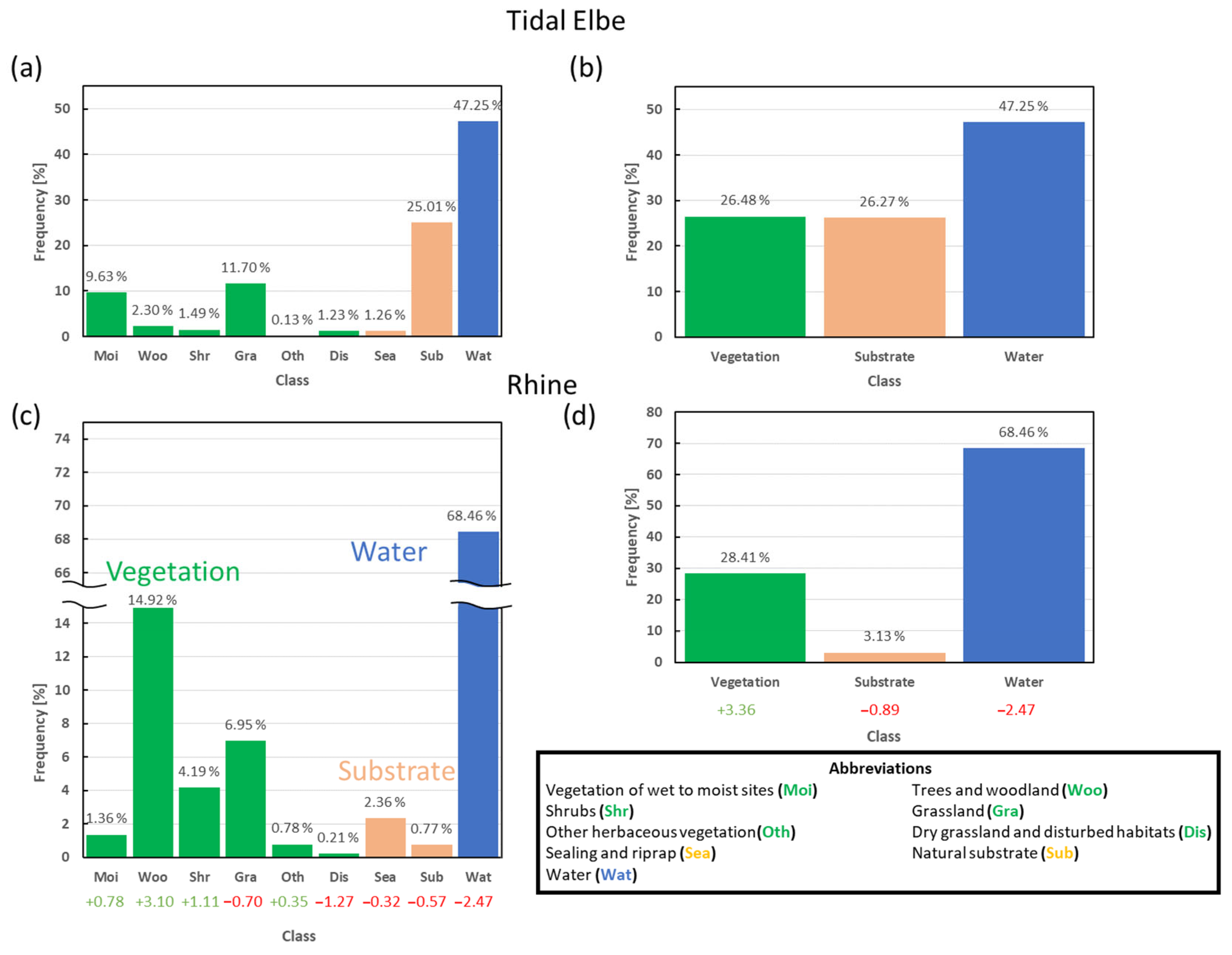
2.1. Study Areas

This study used existing large-scale high-resolution aerial image datasets from riparian zones from the two most important waterways in Germany, the Rhine and the Elbe River, for applying the DL-classification workflow. Areas were chosen where suitable reference data (also called ground truth) exist. The first study area is the Elbe estuary, located in northern Germany, around Hamburg (Figure 1a), and is characterized by tidal flats and marshes. The reference dataset covers 81 km of the Elbe estuary and was collected as part of the fairway modification. In the present study, these data were used to train (with hyperparameter tuning) several CNNs, to analyze the contribution of the different inputs, to calibrate the model confidence and to test approaches to fuse different input modalities.

The second study area covers the river banks of 19 km of the Rhine River in the south-west of Germany, near Mainz (Figure 1b). The vegetation reference data were collected for the purpose of ecological maintenance of the waterway. The second area is used to test the generalization ability of the best-performing model from the first area. Here, the effects of pre-training and the correction of ground truth labels were analyzed.

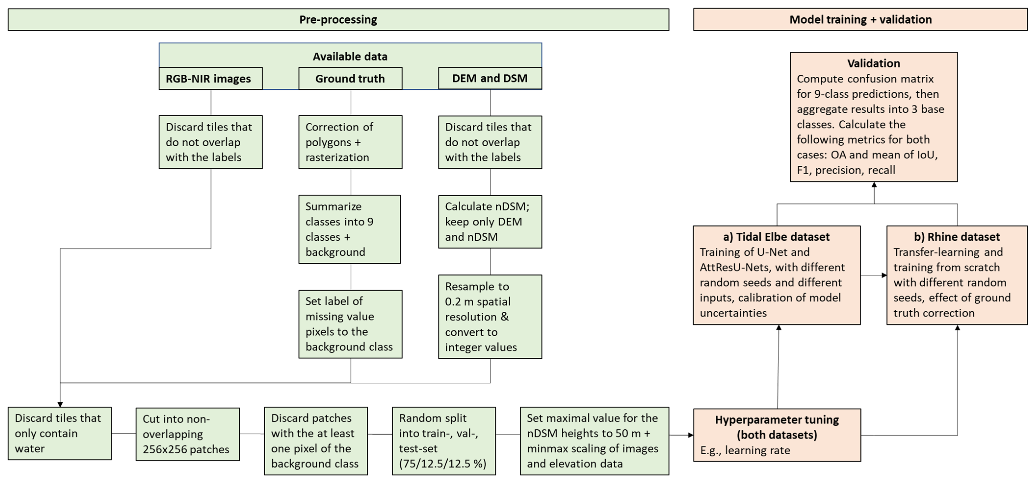
2.2. Data and Pre-Processing

The available data of the tidal Elbe estuary consist of 392 tiles of RGB-NIR aerial images, digital elevation models (DEM) and digital surface models (DSM), all recorded and processed by BSF Swissphoto GmbH (Glattpark in Switzerland). The optical images were captured with an UltraCam Eagle 100 (manufactured by WILD GmbH, Völkermarkt in Austria) on four days between 20 July and 8 September 2016. They have a spatial resolution of 0.2 m, an extent of 5000 × 5000 pixels and are provided as 8-bit (per channel) unsigned raster data. The aerial image data were collected at low tide with outgoing water during a spring tide. The vegetation on the banks of the tidal Elbe grows above the neap high water [55] (mainly in the upper third of the tidal flats). The elevation data were captured with a Trimble AX60 camera (manufactured by Trimble Inc., Westminster, CO in the USA) between 16 March and 1 April 2016. They have a spatial resolution of 1 m and are provided as 32-bit (signed float) raster files.

Reference data (ground truth) for the tidal estuary were originally produced in 2017, also including the above-mentioned remote sensing data in an intermediate step. A Sequential Maximum a Posteriori algorithm produced a pre-classification based on previous field surveys (2006 and 2011). The results were cross-checked and corrected by extensive new field surveys of the whole area in 2016/2017. In this way, 37 classes were mapped [56] and are now used as our reference data.

The RGB aerial images of the Rhine area were captured on 13 August 2012 and 17 September 2013. Overall, 47 tiles with a size of 5002 × 5002 pixels and a spatial resolution of 0.2 m were provided by the BKG (Federal Agency for Cartography and Geodesy, Frankfurt am Main, Germany, [57]). The ground truth data for the Rhine River are based on a vegetation survey of biotope types of the Rhine River from 2016 to 2017 [58].

Both datasets were pre-processed in a similar way (Figure 2). First, image tiles and elevation tiles (DEM and DSM) that did not overlap with the labelled area were discarded. In the next step, the reference data were rasterized to the same dimensions and resolution as the optical image tiles. Thus, the reference data were converted to 8-bit tiles of size 5000 × 5000 pixels (for the Rhine dataset 5002 × 5002 pixels) with a spatial resolution of 0.2 m. The labelled classes were summarized into nine classes, which can be further summarized into three base classes: vegetation, substrate and water (

Table 1. Classes that were considered in this study.

Class	Description
Vegetation of wet to moist sites (Moi)	Vegetation in the immediate vicinity of rivers and lakes. Example units: reed, pioneers, perennials of moist locations
Natural substrate (Sub)	Areas without sealing or vegetation. Example units: sand, gravel, fine-grained material, tidal flats, un-sealed roads
Trees and Woodland (Woo)	Woody vegetation with a height of >3 m. Example units: deciduous forest, hardwood meadow. Example species: Salix spp., Populus spp.
Shrubs (Shr)	Woody vegetation with a height of <3 m
Water (Wat)	Rivers, lakes, ponds
Grassland (Gra)	Vegetation dominated by grasses. Example units: pasture, grassland of intensive or extensive usage
Other herbaceous vegetation (Oth)	Non-woody, herbaceous vegetation at nutrient-rich sites. Example species: Rubus spp., Urtica dioica
Dry grassland and disturbed habitats (Dis)	Example units: medium to tall forbs of dry sites. Example species: Calamagrostis epigejos, Artemisia vulgaris
Sealing and riprap (Sea)	Example units: rocks, buildings, roads

).

Unlabeled pixels were assigned to a separate class (called “background”), which was not considered for the model training. Furthermore, for areas in the tiles that were not captured in the optical images, the corresponding pixels in the ground truth were also set to the background class. Annotation errors in the ground truth can have a significant negative influence on the performance of DL models [42]. Thus, since noticeable labeling errors were observed in the Rhine dataset, the ground truth data were corrected manually. The label of about 15% of the pixels was corrected. Figure 3 shows two examples of uncorrected and corrected ground truth images in the Rhine dataset to illustrate the errors in the original ground truth. Here, some features (like the bridge in Figure 3a,b) were not labelled, or their boundaries were not delineated correctly (e.g., the trees in Figure 3d,e).

The normalized DSM (nDSM) was calculated by subtracting the DEM from the DSM. All negative values in the nDSM were set to 0. The DSM was not considered in further analysis. DEM and nDSM were resampled to a spatial resolution of 0.2 m, and the 32-bit (signed) floating-point values were multiplied by 100 (to conserve the precision of two decimal places) and converted to 8-bit (unsigned) integer values. This step was needed, since the data loader of the Tensorflow library natively needs 8-bit integer values for images with three or four channels.

In the next step, all tiles that only contained the water class were removed to mitigate the class imbalance. This affected 28 tiles for the tidal Elbe and none for the Rhine River. The remaining tiles were cut into 256 × 256 pixel-sized patches, which did not overlap to avoid data leakage during the training and testing of the models. Patches that contained the background class were removed to ensure that only patches with a densely labelled ground truth (with the nine classes) remain. The remaining patches were randomly assigned to three datasets for training the models (training set, about 75%), tuning the hyperparameters (validation set, about 12.5%) and evaluating the final model performances (test set, about 12.5%). In the nDSM, values greater than 50 m were set to 50 m to remove implausible and erroneous values. Afterwards, the values in the nDSM, DEM and RGB(-NIR) patches were scaled in a range between 0 and 1, using the min-max normalization:

$$x^{\prime }={\displaystyle \frac{x-x_{min}}{x_{max}-x_{min}}}$$

(1)

With the original value (x), the normalized value (x′) and the minimum (x_min) and maximum value (x_max) in the training dataset.

Table 2. Detailed information about the datasets used in this study.

Dataset	Number of 256 × 256 Tiles			Modalities	Number of Field Survey Classes	Number of Large Images
	Training Set	Validation Set	Test Set
Tidal Elbe	63,327	10,772	10,545	RGB-NIR, DSM, DEM	37	392
Rhine	4312	773	742	RGB	271	47

Each dataset was split into a training, validation and test set.

summarizes details regarding both datasets.

The class distribution of both datasets (after the pre-processing, before splitting into training, validation and test sets) exhibits a large class imbalance and is illustrated in Figure 4.

2.3. Classification Algorithms

2.3.1. Basics of CNNs

The basic operation giving a CNN its name is the convolution, where an input is convolved with a spatial filter to extract information. For example, one could consider an RGB image with dimensions 256 × 256 × 3 (the numbers correspond to the height, width and number of channels of the image) as an input to a CNN. A filter could have the dimensions 3 × 3 × 3 (usually a 2D convolution is applied, where the number of channels of the filter is equal to the number of channels of the input). Note: both the image and the filter are represented as matrices for conducting the calculations. The result of applying one filter to an input is one feature map, where only one characteristic (also called feature) of the input is detected and displayed (e.g., all edges in the input with a vertical orientation). The parameters of the filter determine which feature is detected (these parameters are learned during the training of the network, i.e., there is an automatic selection of a suitable filter for a given task). The resulting feature map usually has the same spatial dimensions (i.e., height and width) as the input (this is usually ensured by padding the input with zeros). Thus, here, the dimensions of one feature map would be 256 × 256 × 1. Multiple filters are applied by the network to obtain multiple feature maps that detect different characteristics in the input. In this example, if 64 filters were applied to the input, the result would be 64 feature maps, each with dimensions 256 × 256 × 1 and each displaying another characteristic of the input. When more filters are applied, more relevant features can be captured and utilized by the network. All feature maps can be summarized in one matrix, in this example with dimensions 256 × 256 × 64 (the number of channels corresponds to the number of applied filters). CNNs are hierarchically organized in different levels, i.e., the calculated feature maps from one level are the inputs for the filters in the next level. Thus, the characteristics detected by the filters are getting more complex and specialized with subsequent (deeper) levels. This allows the network to learn filters that detect complex characteristics that are specific for each class, allowing the network to solve the desired task (e.g., the semantic segmentation of the input). An introduction to CNNs can be found, for instance, in the references [59,60,61,62].

2.3.2. U-Nets

The U-Net is a CNN that was originally developed for the semantic segmentation of medical images [63]. Several studies demonstrated the potential of U-Net-based architectures for processing remote sensing data [25,27,30,49,64,65]. U-Nets are among the most popular CNNs for the semantic segmentation of vegetation in remote sensing data [7].

Details about the architecture of a basic U-Net can be found in [63]. This study applies the U-Net architecture with the following modifications: residual connections (with batch normalization), attention gates and either early or late fusion of the input modalities. The modifications are described in the following passages. The U-Net, where the architecture is extended by implementing attention gates and residual connections, is referred to as AttResU-Net. The most complex architecture (AttResU-Net with late fusion) is presented in the last section of this sub-chapter.

2.3.3. Residual Connections

Residual connections allow one to efficiently train deeper networks [66]. The residual convolution block is illustrated in Figure 5b. In the main branch, the input feature maps are processed by a convolutional layer. Then, a normalization—the so-called batch normalization—is applied, since it was shown to be beneficial for training deep neural networks (e.g., by enabling faster and more effective optimization and improving the generalization ability [67,68]). The number of channels is increased (usually double the number of input channels). Then the rectified linear unit (ReLU, [69,70]) activation function is used (in this activation function, all negative values are set to zero, and positive values are not modified), and another convolutional layer with batch normalization is applied. In the secondary branch, a 1 × 1 convolution (with batch normalization) is applied to the input feature maps to increase the number of channels. The outputs of the branches are combined by a connection (called residual connection), which adds the feature maps elementwise. Finally, the ReLU activation function is applied to generate the output of the residual convolution block. The convolutions in the main branch have a filter size of 3 × 3, a stride of 1 and use “same” padding (i.e., after applying the convolution to an input, the height and width of the resulting feature maps is the same as the input dimensions). Figure 5a also shows a convolutional block without the residual connection. This block was used in the baseline U-Net architecture.

2.3.4. Attention

The applied attention gate was proposed by Oktay et al. in 2018 [71]. However, there are various ways to design attention modules (e.g., [72,73,74,75]). When incorporated into the U-Net architecture, attention mechanisms showed promising results [65,71,72]. This module allows the network to highlight important sections of the feature maps (and reduces noisy activations or low activations from irrelevant regions) [71]. Here, the attention is used in the skip-connections, which connect feature maps from the encoder (with higher spatial resolution but simpler features) with feature maps from the decoder (with less spatial resolution but more complex features).

Figure 6 shows the structure of the implemented attention gate. Since the feature maps from the encoder and decoder have different heights, widths and number of channels, both inputs must be processed to have equal dimensions. The first input to the attention gate comes from the encoder. Feature maps from the encoder have a higher spatial resolution, but fewer channels (shallower features). A 3 × 3 convolutional layer (with stride = 2 and batch normalization) is applied to lower the spatial dimension. The gating signal comes from the feature maps of a lower stage of the decoder. These feature maps have a lower spatial dimension but contain more complex features and a higher number of channels. Thus, a 1 × 1 convolutional layer (with batch normalization) is applied to reduce the number of channels. In the next step, the processed feature maps from the encoder (with higher spatial information) and decoder (with more complex features) are combined by applying an elementwise addition. Weights that align between both inputs result in higher values. Then, a ReLU activation function is applied to discard negative values. A 1 × 1 convolution is applied to combine the information across all channels into a single channel. In the next step, a sigmoid activation function is applied to scale the values between 0 and 1. Pixels with high values in the resulting feature map correspond to regions with high activations in the feature maps from the encoder and decoder. The dimensions of these attention scores are then processed to match the dimensions of the input from the encoder by applying a transposed convolution (to match the spatial dimensions) and then copying the channel (to match the number of channels). In the next step, the attention scores are elementwise multiplied with the input from the encoder. This step weights the feature maps of the encoder according to the calculated attention weights. The output of the attention gate is obtained by applying a 1 × 1 convolution (with batch normalization).

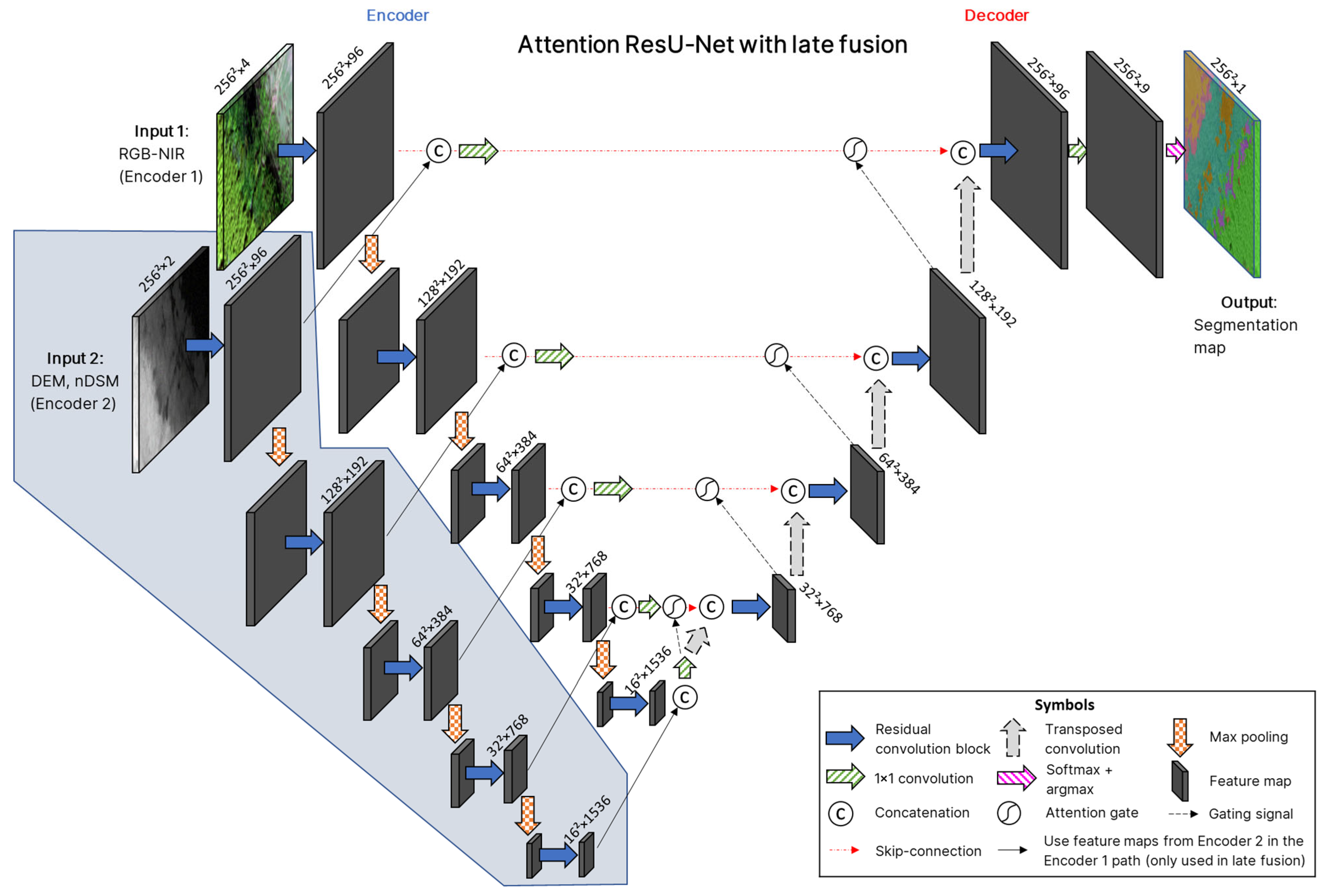
2.3.5. Model Architecture with Early and Late Fusion

The architecture used in this study (Figure 7) is based on the classical U-Net [63], modified with residual connections [66] and an attention gate [71]. Additionally, the fusion approaches presented in [48] are adopted for the combination of the RGB-NIR images and elevation models (nDSM and DEM). From here on, this architecture with late fusion is referred to as AttResU-Net LF. For comparison, one early fusion and one late fusion approach were applied for the fusion of the two modalities. The data from the elevation models were aligned to the RGB-NIR images in the pre-processing. Thus, for the early fusion approach, the data from both modalities could be concatenated and jointly used as the input to the models. In the late fusion approach, both modalities were processed by a separate encoder. The feature maps from both encoders were fused in each stage of the U-Net (similar to the approach of Qiu et al. [48]). Details regarding the model architecture are described below (also see Figure 7).

The basic structure of the AttResU-Net LF consists of an encoder part (per input modality), where features are extracted and the spatial dimensions are downsampled, and a decoder part, where the feature maps are upsampled to the original spatial dimensions and utilized to make the predictions. The encoder and decoder are organized in multiple stages. Feature maps are computed in the encoders by applying convolutional layers (see Figure 5b) to the input. The number of extracted features depends on the number of filters used in the convolutional layer. The filters used in the residual convolutional blocks use a window size of 3 × 3 (and 1 × 1), a stride of 1 and ‘same’ padding. Non-linearity is introduced by applying a ReLU activation function to the feature maps. In each stage of the encoders, one residual convolutional block (see Figure 5b) is applied. At this point, the feature maps from both encoders are used in two paths: (I) the path connecting encoder and decoder (skip-connections, see below): here, the feature maps of both encoders are concatenated to combine the extracted information from the optical images and elevation models. The number of channels is reduced by applying a 1 × 1 convolution. This reduces the computational load of the late fusion approach. (II) In each encoder, the spatial dimensions of the feature maps are downsampled by a factor of two, and the result is passed to the next stage of the corresponding encoder. The downsampling is done by applying a max-pooling layer with a window size of two and a stride of two. The downsampling of the feature maps provides several advantages, including the following: (I) fewer computational resources are needed; (II) only important information is kept in the feature maps; and (III) the receptive field of the convolutional kernels is increased [76,77,78].

In the next stage, again one convolutional block (with twice the number of filters used in the previous stage) is applied, and the resulting feature maps are passed to the skip-connection in the current stage and downsampled to reach the next stage. Thus, in the stages of the encoders, the spatial size of the feature maps decreases while the number of features increases. This procedure is repeated four times until the main connection (bridge) between the encoders and decoder is reached. Feature maps in the bridge are processed by a convolutional block but not downsampled.

The feature maps from both encoders are concatenated and then used simultaneously in two ways: (I) A transposed convolution is applied to upsample the spatial dimensions. (II) As input to the attention gate (see Figure 6) in the skip-connections of the previous stage in the encoder (which connect encoders and decoder) to improve the feature maps in the decoder (by combining the high-resolution features with the upsampled feature maps [63]). The results of both operations are concatenated. Thus, information of both encoders and the decoder is combined here. Then, a residual convolutional block (with half of the number of filters used in the previous stage) is applied. Thus, the operations in one stage of the decoder can be summarized as follows: the feature maps are passed to the attention gate and upsampled. Then, the feature maps are concatenated and a residual convolutional block is applied. Therefore, in subsequent stages of the decoder, the spatial size of the feature maps increases again, while the number of feature channels decreases.

This procedure is repeated until the spatial size of the input is restored (note: in the original architecture of the U-Net, the convolutions were applied without padding; thus, in this case, the size of the final feature maps is slightly lower). Then, a 1 × 1 convolutional layer is applied, where the number of filters (with a window size of 1 × 1) is equal to the number of classes that are considered in the classification (here: nine). Finally, the softmax activation function is applied to the feature maps (for a binary classification, a sigmoid function would be used). This rescales the pixel values in the feature maps: each pixel has a value between 0 and 1, and at a fixed position, the sum of the pixel values over each channel equals 1. The semantic segmentation map is obtained by applying the argmax of the feature maps. The pixel value in the semantic segmentation map is set to the class with the corresponding channel that exhibits the highest softmax (or sigmoid) score at this position.

The encoder for the input of the elevation models (“encoder 2” in Figure 7) is only used in the late fusion approach. For the early fusion models (called AttResU-Net EF), there is only one encoder that processes all data together (RGB-NIR, DEM, and nDSM are concatenated). Since this approach has considerably fewer trainable parameters, two architectures were considered for the early fusion. The first one has the same number of filters in each stage of the encoder as the late fusion encoders (96 filters in the first stage, EF1). The second architecture has 123 filters in the first stage, resulting in a similar number of trainable parameters as the AttResU-Net LF (EF2).

2.4. Accuracy Measures

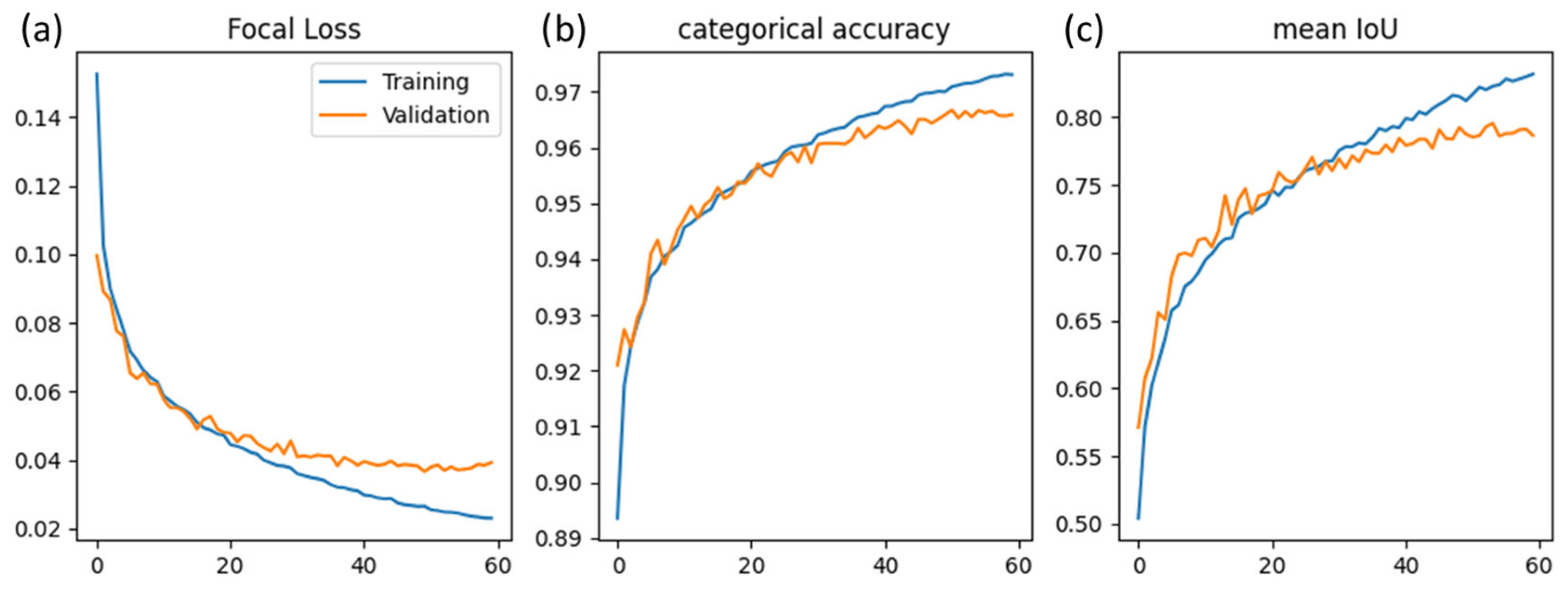
To assess the performance of the trained models, for each classification, the multi-class confusion matrices were computed. The confusion matrix is a tool to compare the predictions of a model with the ground truth for each class. The entries of a confusion matrix can be summarized as true positives (TP), true negatives (TN), false positives (FP) and false negatives (FN). Based on these four components, various metrics can be derived. For this study, the most common metrics for the application of DL for the semantic segmentation in remote sensing images were calculated for each class separately: Precision, Recall, Intersection over Union (IoU) and F1-Score [79,80]. For each metric, the mean value of all classes is calculated by using the arithmetic mean. Furthermore, the overall accuracy (OA) was calculated as an additional metric, which summarizes the performance over all classes.

The OA was calculated by dividing the sum of the TP values of each class (i) by the number of predictions (n). Due to this calculation, the OA is sensitive to imbalanced class distributions [80].

$$OA={\displaystyle \frac{{\sum }_{i}TP}{n}}$$

(2)

The precision (also called the user’s accuracy for positives, in traditional RS literature) is calculated as the ratio of TP to all predictions of a given class.

$$Precision={\displaystyle \frac{TP}{TP+FP}}$$

(3)

The recall (also called producer’s accuracy for positives, in traditional RS literature) is calculated as the ratio of TP to all occurrences of a given class in the ground truth.

$$Recall={\displaystyle \frac{TP}{TP+FN}}$$

(4)

The F1-Score (also called Dice-coefficient) is calculated as the ratio between precision and recall of a given class, where FN and FP are equally weighted:

$$F1-Score={\displaystyle \frac{2\times Precision\times Recall}{Precision+Recall}}$$

(5)

The IoU (also called Jaccard index) is calculated as the ratio between TP and the sum of TP, FP and FN of a given class:

$$IoU={\displaystyle \frac{TP}{TP+FP+FN}}$$

(6)

All metrics range between 0 and 1, where 0 indicates the worst and 1 the best possible performance of the model. A comprehensive discussion of common metrics and their use in remote sensing studies is provided in Maxwell et al. (2021) [79,80].

In addition to these performance measures, the model uncertainty can be investigated. Raw outputs of the final softmax (in a multi-class case) activation function (which takes values between 0 and 1) of complex CNNs usually do not reflect true uncertainties. Modern CNNs are often overconfident classifiers (i.e., true uncertainties are underestimated). This is due to various reasons, including the use of batch normalization and the increasing depth and width of the networks [81]. While the use of the focal loss can decrease this deviation, this can also lead to models that are underconfident (i.e., true uncertainties are overestimated) [82]. A common metric to measure the calibration of a network is the expected calibration error (ECE) [81]. To calculate the ECE, the confidence values of the model predictions are grouped into M equally spaced bins B. Then, a weighted average is calculated over each bin according to the following:

$$ECE=\sum _{m=1}^M{\displaystyle \frac{\left|B_m\right|}{n}}|acc(B_m)-conf(B_m)|$$

(7)

With the number of predictions (n), the number of predictions in the current bin m ($B_m$), the average accuracy of the predictions in the current bin (acc($B_m$)) and the average confidence in the current bin (conf($B_m$)). For a perfectly calibrated classifier, the accuracy would equal the confidence for each bin (e.g., 85% of the predictions in the confidence bin 80–90% would be true predictions). A lower ECE corresponds to a better-calibrated model. A simple calibration method is temperature scaling (an extension of Platt scaling) where the softmax values are scaled by a parameter called temperature. The temperature can be optimized on the validation set by minimizing a loss with respect to the scaled softmax values and the true prediction class. The temperature scaling does not change the class predictions of the model [81].

2.5. Model Training

The choice of hyperparameter (parameters that are not optimized during backpropagation) values has a considerable influence on the performance of models. There are no default values of hyperparameters that lead to optimal results for every architecture and task [83]. Thus, to ensure a fair comparison between the simple U-Net and the AttResU-Net, the hyperparameters were tuned for each architecture (and input) separately. The tuning was conducted with the training and validation sets of the tidal Elbe dataset. A mixture of manual and automatic tuning was applied.

Table 3. Hyperparameters considered in the analysis.

Hyperparameter	Variation	Best Settings for the U-Net Models
Learning rate	Initial LR: 1 × 10−5, 5 × 10−5, 1 × 10−4, 5 × 10−4, 1× 10−3 Decay schemes: none, step decay (Step size: 3, 4, 5, 6, 7; decay rate: 0.7, 0.75, 0.8, 0.85, 0.9)	1 × 10−4 with a step decay (5, 0.8)
Batch normalization (BN)	With/without Momentum parameter: 0.7, 0.75, 0.8, 0.85, 0.9	With BN, momentum = 0.85
Optimization Algorithm	Adam RMSprop SGD	Adam
Loss function	Focal loss (gamma = 2) Cross-entropy loss Dice loss	Focal loss
Number of stages in the U-Nets (without the bridge)	3, 4	4
Dropout layer	Without/with: 0.1, 0.2	Without
Parameter initialization	Random He-normal	He-normal
Number of Epochs	Up to 100	60
Upscaling	Transposed convolution Upsampling (nearest neighbor)	Transposed convolution
Activation function	ReLU Leaky ReLU (alpha = 0.1)	ReLU

Overview of the optimized hyperparameters of the DL architectures for the semantic segmentation of the Tidal Elbe dataset. In bold: tuned with the hyperband algorithm; the other hyperparameters were tuned manually. For all U-Nets, the same set of optimal hyperparameters was determined.

shows the tuned hyperparameters and the variation that was considered. For hyperparameter settings not discussed here or where no range of values is given, the standard values were used (e.g., for the Adam optimizer). The manual tuning was conducted to select well-working options for the following hyperparameters:

• The loss function (used to quantify the deviation of the model predictions and the ground truth values).
• The optimization algorithm (used to adapt the model weights during training to minimize the loss).
• The initialization of the parameters in the convolutional layers.
• The upsampling method used in the decoder of the U-Net to increase the spatial size of the feature maps.
• The activation function (used to introduce non-linearity into the network).

Data augmentation (flipping and mirroring) was applied to the training data to improve model performance [84]. Furthermore, a batch size of 32 and a patch size of 256 pixels were set to ensure that the large models could be trained on the available computational resources. The number of filters in the convolutional layers was set to the maximum value possible in the late fusion architecture with the available computational power (96 in the first stage of the U-Nets).

The automatic tuning was conducted on a few selected hyperparameters (highlighted in bold in Table 3): the momentum in the batch normalization layer, the initial learning rate and the corresponding decay scheme (step size and decay rate). These were chosen for the automated tuning due to the high number of plausible values and since they had a noticeable influence on the model performance. The implementation of the hyperband algorithm [85] in the Keras-Tuner library [86] was utilized for the automatic hyperparameter tuning. For each of these hyperparameters, the hyperband algorithm randomly chose a value from the predefined values (given in Table 3). The settings with the highest performance (in terms of, e.g., mean IoU) on the validation set were used for training the final models (see Section 3.2). The final performance of the models with the best hyperparameters was evaluated on the test set. Furthermore, the influence of different input modalities (RGB, NIR, DEM, and nDSM) on the performance was analyzed. The usage of the optical images and height information was investigated by testing early and late fusion strategies. All models were trained for 60 epochs. The models with the highest performance on the validation set were saved and used for further analysis.

Transfer Learning

Instead of training a new DL model from scratch (with randomly initialized weights) for every new task and dataset, it is possible to adapt existing models by using transfer learning. In transfer learning, the knowledge learned on one (usually relatively large) dataset (or task) is re-used to boost the performance on a related task or (usually small) dataset. This is done by training (also called pre-training) an existing model on another dataset (this is called fine-tuning). There are multiple strategies for applying transfer learning [87,88].

The AttResU-Net, which was trained on the tidal Elbe dataset (only with the RGB images), was applied for the classification of the Rhine dataset. To assess the effect of fine-tuning and the correction of the ground truth, the model was applied without fine-tuning and with fine-tuning on the uncorrected and corrected ground truth. Furthermore, an AttResU-Net with randomly initialized weights was trained from scratch. Hyperparameter tuning was conducted to determine suitable values for the learning rate (and decay scheme).

All models were implemented with the TensorFlow (2.13.0, ref. [89]) and Keras (2.13.1, ref. [90]) libraries. The U-Net implementations are based on [91] and were heavily modified for this study (e.g., by adding the late fusion approach and adapting the attention implementation). All computations were performed on an NVIDIA RTX A6000 (48 GB memory, with CUDA 11.8). For the model training, deterministic GPU calculations were used, and all random seeds were set to a fixed value of 2. To assess the variation of the results due to random processes (e.g., initialization of the weights), each model was also trained with three other fixed random seeds (1, 3 and 4).

3. Results

This section is structured as follows: first the tidal Elbe dataset was used to train (with hyperparameter tuning) a simple U-Net and AttResU-Net and compare their performance on the test-set. The AttResU-Net was used for further analysis: the contribution of the different inputs, the calibration of the model confidence and evaluation of the early and late fusion of the two input modalities (optical images and elevation models). Then, the dataset of the Rhine River was used for testing the generalization ability of the best-performing model. Furthermore, the correction of ground truth labels and the effect of pre-training were analyzed. To assess the variation of the performance metrics, each model was trained with four different random seeds.

3.1. Hyperparameter Tuning

Table 3 summarizes the tested hyperparameters (with the considered range of settings) and the best settings for the U-Nets. The tuning resulted in the same optimal settings for all of the tested U-Nets: a learning rate of 1 × 10⁻⁴ with a step decay (step size of 5 epochs and a decay rate of 0.8), batch normalization (with a momentum of 0.85) and the Adam optimizer was used. Of the tested loss functions, minimizing the focal loss (implemented in the focal loss library, version 0.0.7 [92]) was best suited for training the models. The focal loss was shown to be effective in dealing with imbalanced classes [93] and is defined as the cross-entropy loss multiplied by a modulating factor:

$$Focalloss={-(1-p_t)}^{\gamma }\times \mathrm{l}\mathrm{o}\mathrm{g}\left(p_t\right)$$

(8)

With the model’s estimated probability for the ground truth class p_t and the gamma value γ, which reduces the impact of easy-to-classify examples on the loss. With γ = 0, the focal loss is equal to the cross-entropy loss. Higher values for γ extend the range in which easy examples receive low loss values (thus, difficult examples contribute more to the loss). A typical value for γ is 2 [92,93]. The architectures consist of four stages (plus the bridge between encoder and decoder) and apply the ReLU activation function, He-normal parameter initialization in the convolutional layers and the transposed convolutional layer for upsampling the feature maps. Dropout layers were not beneficial for the model performance.

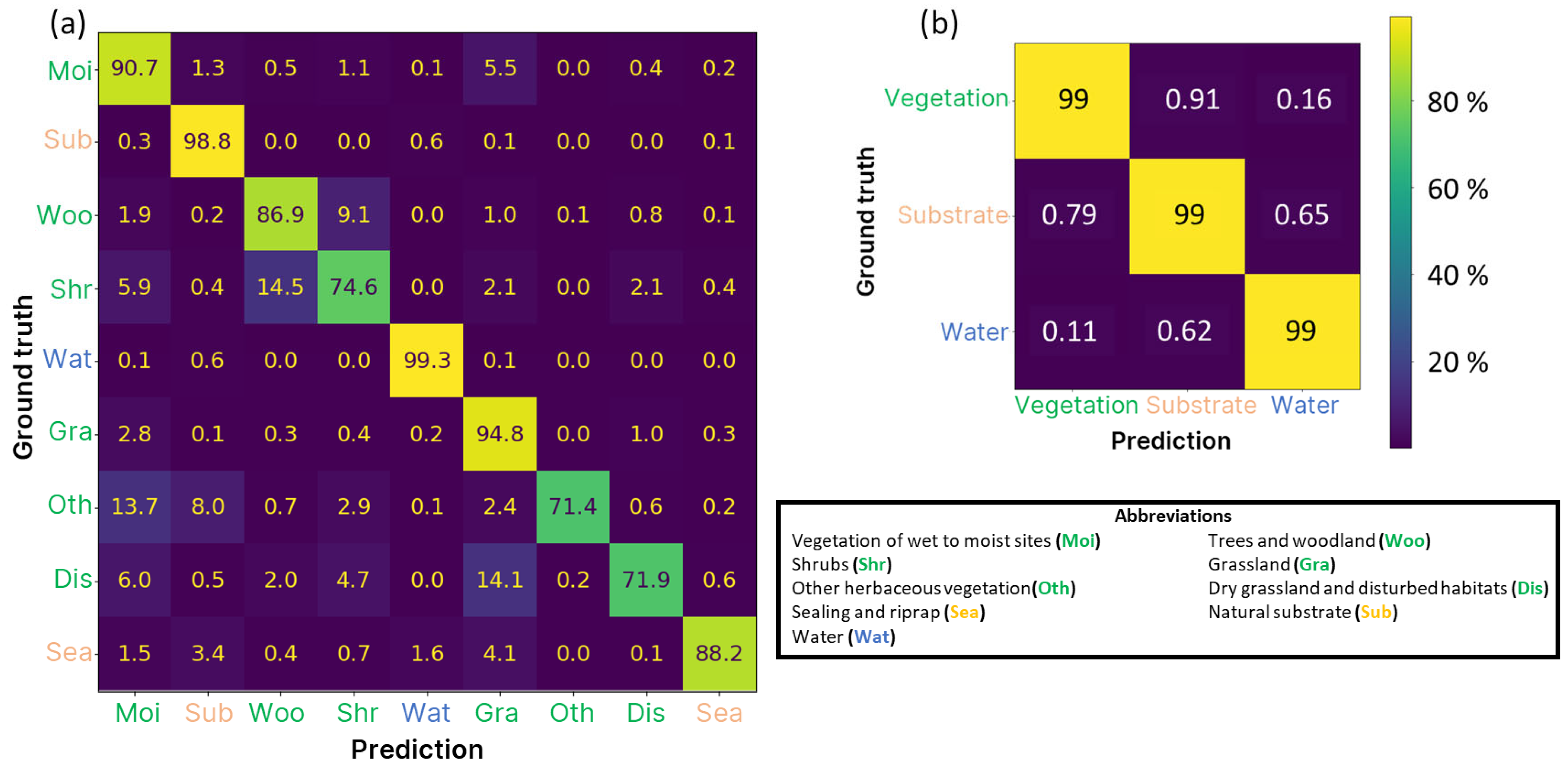
3.2. Performance on the Tidal Elbe Dataset

The performance of the trained models was evaluated on the test set of the Tidal Elbe dataset (

Table 4. Performance of the trained models on the Tidal Elbe dataset (nine classes).

Input Data Modality	Mean IoU	Mean F1-Score	Overall Accuracy	Mean Precision	Mean Recall	Training Duration per Epoch [s]	Number of Trainable Parameters
U-Net
RGB-NIR	75.05 74.74–75.23	84.69 84.50–84.81	96.00 95.87–96.07	86.83 86.23–87.43	83.23 83.02–83.44	~1755	69,834,249
AttResU-Net
RGB	75.41 74.97–75.80	84.97 84.61–85.27	96.03 95.97–96.08	87.13 87.07–87.27	83.51 82.98–83.96	~2398	78,472,545
RGB-NIR	76.47 76.23–76.73	85.75 85.57–85.89	96.32 96.29–96.36	87.55 87.44–87.78	84.39 84.21–84.49	~2406	78,473,505
RGB, DEM, nDSM	77.91 77.56–78.19	86.82 86.57–87.02	96.43 96.37–96.49	88.20 87.59–88.51	85.39 85.39–85.87	~2567	78,474,465
DEM, nDSM	65.71	77.42	93.49	80.84	75.28	~2493	78,471,585
RGB-NIR, DEM, nDSM (EF1)	77.68 77.49–77.87	86.60 86.46–86.75	96.55 96.52–96.58	87.75 87.50–88.03	85.64 85.55–85.71	~2650	78,475,425
RGB-NIR, DEM, nDSM (LF)	77.81 77.53–78.12	86.73 86.51–86.92	96.49 96.44–96.54	88.55 88.16–88.96	85.40 85.04–85.83	~3486	128,741,601
RGB-NIR, DEM, nDSM (EF2)	78.33 77.96–78.66	87.08 86.81–87.31	96.61 96.58–96.64	88.30 87.26–88.81	86.13 85.51–86.43	~3901	128,805,018

The metrics were determined by calculating the arithmetic mean of all individual runs. Below each performance metric, the range across the four tested random seeds is given (except for the model trained only on DEM and nDSM). The best and second-best values are highlighted in bold and underlined numbers, respectively. For the combination of optical images with elevation models, an early fusion (EF) and a late fusion (LF) approach were tested.

). To consider the variation of the performances, each model was trained four times with different random seeds and evaluated on the test set. The final performance of a model was then obtained by taking the arithmetic mean of these performances. Each model was trained with the same four random seeds. With RGB-NIR images as input, the simple U-Net reached an average mean IoU of about 75%. Including attention and residual connections in the architecture improved the performance to an average of 76.47% (depending on the random seed, the improvement ranges between 1.00 and 1.99 percentage points).

The AttResU-Net architecture was trained with different input modalities to assess the performance gain with each additional modality. Without the NIR channel, the performance dropped to an average of 75.41% (about 1 percentage point; depending on the random seed, the performance dropped between 0.43 and 1.76 percentage points). When adding the elevation models to the input (with early fusion of the modalities), the average mean IoU improved by 1.21 percentage points (depending on the random seed, between 0.76 and 1.64) to 77.68% (EF1 model). Additionally, to extend the ablation study and further analyze the influence of the input modalities, one model was trained only with the elevation models as an input. Here, a mean IoU of 65.71% was reached (due to the low performance compared to the other models, only one random seed was considered). Furthermore, one model was trained without the NIR channel (i.e., RGB and elevation models were used as the input). This model slightly outperformed the EF1 model (where the NIR channel was considered) and reached a mean IoU of 77.91%. This is mostly due to better results for the “other herbaceous vegetation class” (with a mean IoU of 62.3% instead of 58.1%), for most classes the IoU slightly decreased without the NIR channel.

Since the overall performance with and without the NIR channel (considering RGB and elevation models as input) is almost identical in our study and the NIR channel has proven to be beneficial in other studies [12,94,95], the successive model trainings include the NIR channel. In the late fusion approach (LF), a second encoder was trained to extract the features from the elevation models. Therefore, the number of trainable parameters and training time increased significantly by about 50 × 10⁶ parameters and about 800 s per epoch, respectively. However, the average mean IoU (compared to EF1) increased only slightly to 77.81% (0.13 percentage points). In contrast to the other results, depending on the random seed, the model with the LF approach performed worse than the EF1 approach (up to 0.34 percentage points) or better (up to 0.63 percentage points).

For a fair comparison between early and late fusion, an early fusion model with a similar number of trainable parameters was trained (EF2). The training duration increased to about 3900 s per epoch, but the model also achieved the highest performance with a mean IoU of 78.33% (0.52 percentage point increase compared to the late fusion model; depending on the random seed, a slight decrease of up to 0.16 or an increase of up to 1.13 percentage points). Overall, the elevation maps as additional inputs led to an increase in the mean IoU of about 1.21 to 1.86 percentage points (between 0.76 and 2.43, depending on the fusion approach and random seed). For the semantic segmentation of the three base classes, the additional input modalities only slightly improved the mean IoU (from 97.19 to 97.75%), and the difference between early and late fusion architectures was neglectable. For the best-performing model, the progress of the focal loss, accuracy and mean IoU during training is shown in Figure 8. The highest performance was reached after 54 epochs.

For the best-performing model (AttResU-Net EF2), normalized confusion matrices were computed for the semantic segmentation of all nine and the three base classes (Figure 9). Three classes (“shrubs”, “other herbaceous vegetation” and “dry grassland and disturbed habitats”) were classified with recall values between 71 and 75%. Two classes (“trees and woodland” and “sealing and riprap”) were detected with recalls of 87 and 88%. For the other classes (“vegetation of wet to moist sites”, “natural substrate”, “water” and “grassland”), recall values over 91% were reached. The largest misclassifications (each with about 14%) were between “shrubs” and “trees and woodland”, “grassland” and “dry grassland and disturbed habitats” and “vegetation of wet to moist sites” and “other herbaceous vegetation”.

For the semantic segmentation of the base classes, the classification results were summarized into the three classes (“vegetation”, “substrate” and “water”). For all three classes, recall values of 99% were achieved (

Table 5. Performance of the trained AttResU-Nets on the tidal Elbe dataset (three classes).

Input Modalities	Mean IoU	Mean F1-Score	Overall Accuracy	Mean Precision	Mean Recall
RGB	97.19 96.90–97.33	98.56 98.40–98.63	98.71 98.57–98.76	98.57 98.43–98.67	98.58 98.43–98.67
RGB-NIR	97.58 97.53–97.60	98.77 98.73–98.80	98.90 98.89–98.91	98.73 98.73–98.73	98.79 98.77–98.80
RGB, DEM, nDSM	97.62 97.57–97.67	98.78 98.73–98.83	98.92 98.88–98.94	98.74 98.70–98.77	98.83 98.80–98.87
DEM, nDSM	94.30	97.07	97.42	96.93	97.23
RGB-NIR, DEM, nDSM (EF1)	97.74 97.70–97.77	98.86 98.83–98.87	98.98 98.97–98.99	98.85 98.83–98.87	98.88 98.87–98.90
RGB-NIR, DEM, nDSM (LF)	97.68 97.63–97.70	98.83 98.80–98.87	98.95 98.94–98.97	98.77 98.73–98.80	98.88 98.87–98.90
RGB-NIR, DEM, nDSM (EF2)	97.75 97.70–97.79	98.87 98.87–98.87	98.99 98.97–99.00	98.84 98.83–98.87	98.89 98.87–98.93

The metrics were determined by calculating the arithmetic mean of all individual runs. Below each performance metric, the range over the four tested random seeds is given. The best and second-best values are highlighted in bold and underlined numbers, respectively.

).

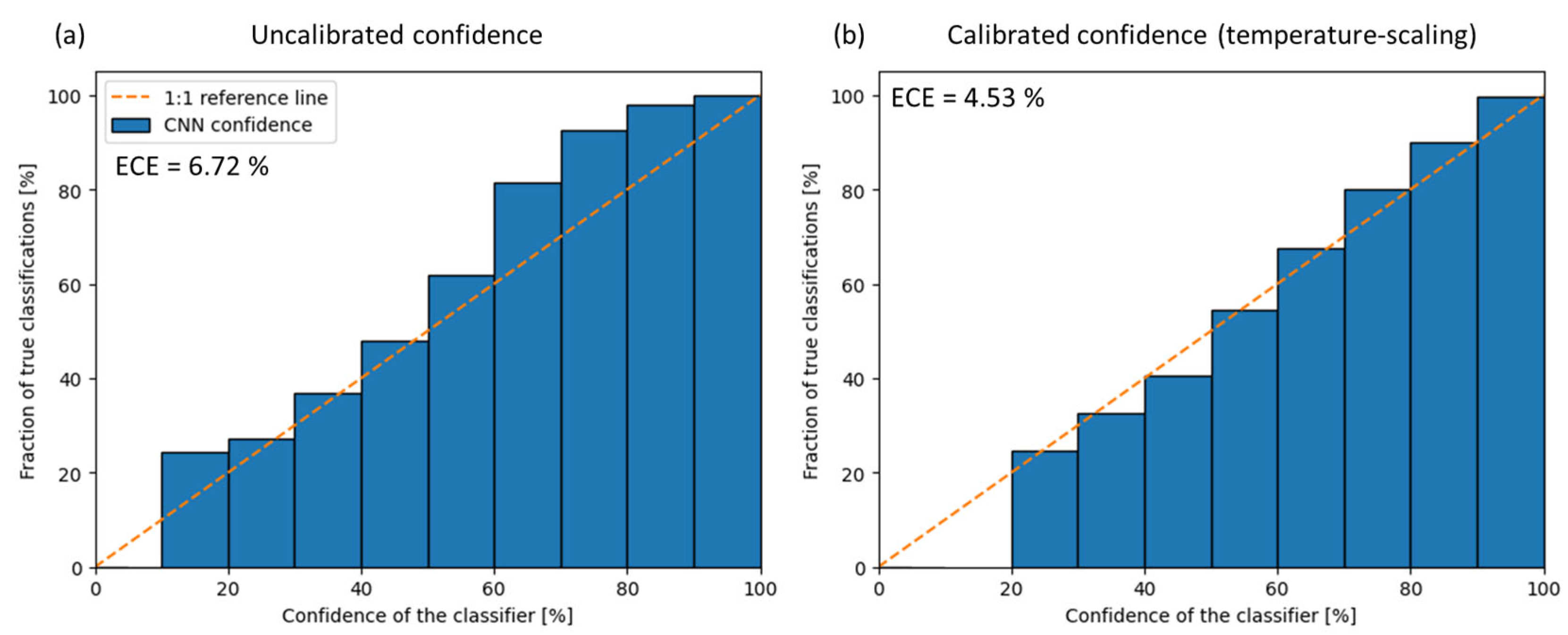
3.3. Model Calibration

To assess the model calibration, reliability diagrams were calculated in the following way. The softmax scores (ranging from 0 to 100%) of the best-performing model (AttResU-Net EF2) were grouped into bins with a width of 10%. For each bin, the fraction of true predictions was calculated. Figure 10a shows the reliability diagram prior to the calibration. The bins between 60 and 90% show a noticeable deviation from the reference line, i.e., the model is underconfident and gives greater uncertainties than the true uncertainties are. The calculated ECE is 6.72%.

The temperature scaling was applied to calibrate the model predictions. The optimal temperature value was determined with the validation set by minimizing the cross-entropy loss with respect to the scaled softmax values and the true prediction class (for 100 epochs). The minimum loss was reached after 55 epochs with a temperature value of about 0.5867. Applying the temperature scaling improves the calibration (especially for the bins between 60 and 90%) and reduces the ECE to 4.53%.

3.4. Performance on the Rhine Dataset (Generalization)

The AttResU-Net, which was trained on the RGB images of the tidal Elbe dataset, was fine-tuned for the classification of the Rhine dataset. The hyperparameter tuning resulted in the following values for the fine-tuning: The fine-tuning (of all layers in the architecture) was conducted for 100 epochs with a learning rate of 5 × 10⁻⁴ and a stepwise decay (decay rate of 0.75 and a step size of 6). The models with randomly initialized weights were trained for 100 epochs (one epoch was completed in about 162 s) with a learning rate of 1 × 10⁻⁴, which was decreased after every third epoch with a decay rate of 0.9. The model with the best performance on the validation set was saved and used for further analysis. The final performance was evaluated with the test set and the corrected ground truth as the reference (

Table 6. Performance of the models on the Rhine dataset.

Classes	Mean IoU [%]	Mean F1-Score [%]	Overall Accuracy [%]	Mean Precision [%]	Mean Recall [%]
Direct application of the AttResU-Net with corrected ground truth data (without fine-tuning)
9	21.85 18.53–24.77	30.32 27.33–33.27	54.66 40.42–69.13	33.48 31.67–36.68	37.65 35.87–39.55
3	46.96 36.50–57.17	63.01 53.50–71.60	67.03 54.16–80.28	65.36 59.83–70.13	71.80 66.40–76.90
Fine-tuning with uncorrected ground truth data
9	38.53 38.42–38.57	49.30 49.04–49.51	88.47 88.29–88.61	56.49 55.51–57.02	52.30 51.96–52.60
3	70.25 70.03–70.50	79.22 79.07–79.43	94.14 94.07–94.26	79.22 79.10–79.47	79.87 79.63–80.13
Fine-tuning with corrected ground truth data
9	59.95 58.83–60.59	72.34 70.98–73.10	93.87 93.82–93.91	77.83 76.54–79.07	69.72 68.20–70.78
3	85.71 85.50–85.93	91.55 91.40–91.69	98.04 97.98–98.06	91.66 91.13–91.83	91.47 91.23–91.67
Training from scratch with corrected ground truth data (randomly initialized weights)
9	58.15 57.72–58.68	70.46 69.92–71.08	93.45 93.07–93.65	76.73 74.12–77.99	67.70 66.76–68.21
3	85.17 84.89–85.37	91.13 90.93–91.27	98.01 97.95–98.05	91.59 91.37–91.83	90.68 90.49–90.77

The table shows the performance of the models (from scratch and pretrained on the tidal Elbe dataset, only with RGB images as the input) on the Rhine dataset for classifying nine and three summarizing classes. The best and second-best values are highlighted in bold and underscored numbers, respectively.

). Each model was trained with four different random seeds. The performance metrics were determined by taking the arithmetic mean of all performance values. Without fine-tuning, the AttResU-Net achieved an average mean IoU of about 22%. The performance increased to about 38% (in terms of average mean IoU) when the model was fine-tuned on the uncorrected ground truth. By using the corrected ground truth as the reference for the fine-tuning, the mean IoU greatly increases to about 60%, which is about 2 percentage points higher than training a model from scratch.

Normalized confusion matrices were computed for the semantic segmentation of the nine and the three classes with the fine-tuned AttResU-Net (Figure 11). The class “dry grassland and disturbed habitats” was classified with a low recall value of 21% (with an average mean IoU of 18%). Five classes (“vegetation of wet to moist sites”, “shrubs”, “natural substrate”, “other herbaceous vegetation” and “sealing and riprap”) were detected with recalls between 56 and 79% (and average mean IoUs between 39 and 65%). For the other classes (“grassland”, “trees and woodland” and “water”), recall values between 86 and 99% (with average mean IoUs of 76–98%) were reached. The largest misclassifications were between “shrubs” and “trees and woodland” (34%) or “trees and woodland” (27%), and between “dry grassland and disturbed habitats” and “grassland” (21%) or “trees and woodland” (22%). The base classes “vegetation” and “water” were classified with a recall of over 97% and average mean IoUs of about 94 and 98%, respectively. A recall of 79% and mean IoU of about 64% was reached for the class “substrate”. The largest sources of errors were the misclassification of “substrate” as “vegetation” (15%) and “water” (6.2%).

4. Discussion

4.1. Random Seeds

To ensure a fair comparison between different models and inputs, hyperparameter tuning was conducted for each architecture (with the different input modalities) separately. Furthermore, each model was trained with four (identical) random seeds. This is important because the hyperparameters and random initializations can have a large influence on the model performance [83,96]. Thus, their influence could make a model comparison meaningless, since, e.g., a better model with an unfavorable random seed could perform worse than a worse model with a favorable random seed. This is highlighted by the results of this study: The variation of the random seed led to a variation of the mean IoU of up to 0.38 and 0.83 percentage points (depending on the model and input). Furthermore, the same random seed resulting in high performance for a U-Net with one input modality did not necessarily lead to a high performance for the other U-Nets (and vice versa). For example, the same random seed led to the highest performance for the AttResU-Net with only RGB images as input (75.80% mean IoU) and the lowest performance for the model with all inputs (EF1, 77.49% mean IoU). This means that even a comparison of one architecture with different inputs is only meaningful if more than one fixed random seed is considered.

4.2. Early vs. Late Fusion

The late fusion of the feature maps extracted from the optical images and the elevation models slightly outperformed the first early fusion approach. However, the late fusion model also had about 64% more learnable parameters. Since CNNs usually perform better with more parameters in the architecture (e.g., with more filters in the convolutional layers [97]), the improvement could be attributed to the implementation of the data fusion or simply the increase in parameters (or both). Thus, to ensure a fair comparison, an early fusion approach with an approximately equal number of learnable parameters was trained. This model outperformed the late fusion approach and thus revealed that the improvement can be attributed to the increasing number of filters in the CNN. Furthermore, for the tidal Elbe dataset, the early fusion seems to be more beneficial than the late fusion approach.

4.3. Model Performance on the Tidal Elbe Dataset

The influence of different input modalities (and fusion strategies) was investigated with the tidal Elbe dataset. Figure 12a presents the IoU per class and model (with different input modalities), averaged over the runs with the different random seeds. The addition of spectral information from the NIR channel improved the IoU for all classes by about 0.28–2.68 percentage points. The largest increase in IoU was for the classes “other herbaceous vegetation”, “vegetation of wet to moist sites”, “sealing and riprap”, “dry grassland and disturbed habitats” and “shrubs”. Several studies demonstrated the benefits of the NIR channel for the discrimination of vegetation (e.g., [12,94,95]). Incorporating elevation data further enhances the IoU, particularly in distinguishing vegetation types with similar spectral signatures but differing heights, such as “shrubs” and “trees and woodland”. Depending on the model, the IoU increased between 0.1 and 3.55 percentage points. For the best-performing model, the greatest increase in the average IoU was for the classes “trees and woodland”, “sealing and riprap”, “other herbaceous vegetation”, “shrubs” and “dry grassland and disturbed habitats” (2.15–3.55 percentage points). The importance of elevation data for classifying riparian vegetation is also emphasized in a related study by Rommel et al. [12]. This is highlighted by a model solely trained on elevation data. This model shows high performance for “trees and woodland” (a recall of 83%) and low confusion with the “shrubs” class (about 18%). The model already detects five classes with high performance (IoU > 70) and four classes with a lower performance (IoUs between 32 and 58%, Figure 12). The elevation models might provide complementary information to the optical images and thus enable a performance boost.

However, training a model only with RGB and elevation models (without the NIR channel) slightly (~0.23 percentage points) improved the overall performance compared to a model (EF1) trained on all inputs. The performance of six classes decreased without the NIR channel (between 0.1 and 0.75 percentage points), whereas the performance of two classes (“dry grassland and disturbed habitats” and “shrubs”) improved slightly (0.05–0.35 percentage points), and the performance of the “other herbaceous vegetation” increased greatly (4.2 percentage points). Since the performance for the “other herbaceous vegetation” increases substantially, the overall performance is greater without the NIR channel.

Adding more information does not necessarily lead to improved model performance [98,99]. Furthermore, a model trained on a selection of channels can outperform a model trained on all available channels [99]. Previous studies reported the ambiguity of the NIR channel. Although it is usually considered useful, the NIR channel may cause a degradation in performance for individual classes [100,101]. In our case, adding the NIR channel and the elevation models to the RGB input individually, both increased the model performance. However, the utilization of all inputs was slightly less beneficial, especially due to the lower performance for the “other herbaceous vegetation”. This effect might be caused by multiple factors, like the low number of training examples or a heterogeneous composition of this class (only influencing the distribution in the NIR channel). A wide-spread distribution of the NIR channel, compared to the RGB channels (Figure 13), supports this hypothesis. The width of the distribution was calculated by considering 90% of the values (discarding the 5% lowest and 5% highest reflection values). The distribution of the NIR channel is between 75 and 100% wider than the other optical channels (this difference is between −0.12 and 57% for the other vegetation classes). The utilization of both, the NIR channel and the elevation models, might introduce conflicting information for the “other herbaceous vegetation” and thereby weaken the corresponding performance.

Overall, most classes benefited from the additional inputs. The difference of the IoUs of the classifications of the simpler model (AttResU-Net with RGB images as inputs) and the best-performing model (AttResU-Net with RGB-NIR images and elevation models as inputs, EF2) revealed that the performance for the minority classes increased the most (Figure 12b). The simpler model already achieved high IoUs for the majority classes (“water” and “natural substrate”), and thus the IoU only increased slightly with the more complex models (less than 1 percentage point). Contrarily, the IoU of the minority classes (“trees and woodland”, “sealing and riprap”, “other herbaceous vegetation”, “shrubs” and “dry grassland and disturbed habitats”) significantly improved with the additional inputs (between about 2 and 6 percentage points, depending on the model). Overall, the models achieved higher performance for classes with more training data and vice versa. Hence, the model performance might be improved by specifically collecting more training data for the minority classes. Since the minority classes benefited the most from more complex model architectures, the detection of these classes might be further improved with increasing model complexity. Despite the large class imbalance, the best model achieves decent classification for the minority classes (with average IoUs between 57 and 62%). For the other six classes, the model reaches high performance (with average IoUs of 76–99%). Furthermore, the classification of the three base classes is in excellent agreement with the ground truth (with IoUs > 99%). Whether the higher effort (e.g., collecting more training data, adding more modalities, using more computational resources) is justified depends on the performance requirements for a given task.

4.4. Model Uncertainties

The reliability diagrams (Figure 10) revealed an overestimation of prediction uncertainties by the model. Usually, CNNs underestimate the uncertainty due to, e.g., the increasing depth and width of the networks [81]. However, the use of the focal loss could explain the opposite behavior of the trained networks [82]. The model predictions provide the most benefit to practical applications if the level of uncertainty can be trusted and appraised by users. Thus, the reliability of DL models should be analyzed in similar case studies and, if needed, predictions should be accordingly calibrated. This study successfully applied temperature scaling for the calibration. This method is effective and easy to implement and apply, which makes it especially suitable for practical applications [81]. The uncertainties can be used to guide in situ campaigns by focusing the manual mappings on areas where the classification exhibits high uncertainties.

4.5. Generalization to the Rhine Dataset

Furthermore, this study analyzed the generalization ability of the trained model for the classification of a second dataset. The DL model is (pre-)trained on the tidal Elbe dataset and then applied to the Rhine dataset, which has significantly less training data (about 93% less data). The direct application of the pre-trained model led to low agreement with the ground truth (about 22% IoU). The generalization is challenging due to various differences in the datasets. These differences include the number of mapped classes in the reference data (which are summarized to nine classes—Table 2), the different areas covered, the different composition of the vegetation (tidal Elbe vs. Rhine), the available data sources and the temporal difference (2016 vs. 2012 and 2013). Figure 14 illustrates the spectral differences of the datasets, exemplary for the “vegetation of wet to moist sites” (Moi) class between the two areas. The distribution of the RGB values differs in the characteristics of the peaks (position, height, ordering) and shape. Since the Rhine dataset is composed of aerial images from two different measurement campaigns (from 2012 and 2013), the spectrum of the “vegetation of wet to moist sites” class shows a slight bimodal shape (Figure 14b). The assemblage of a large and diverse dataset (e.g., from different measurement campaigns) would be beneficial for improving the generalization ability. A model that is pre-trained on an extensive dataset with a large variation is more likely to generalize well to new data [102,103].

Furthermore, the correction of labeling errors demonstrated the importance of a reliable ground truth. A model trained on the original ground truth achieved lower mean IoU (about 20 percentage points) than the model trained on the corrected ground truth. Despite the large differences in the datasets, the pre-training was slightly beneficial in comparison with training from scratch. Despite the large difference between the datasets, the pre-trained model achieved a slightly higher mean IoU (about 2 percentage points).

5. Conclusions

Compared to traditional ML methods, DL offers advantages that include the automatic extraction of meaningful features from data, the handling of large datasets, higher performance in many applications and methods for improving the generalization ability (e.g., transfer learning) [14]. This study demonstrated the capabilities of DL models for a large-scale classification of riparian vegetation with high accuracy. A well-chosen model architecture, with appropriate settings (e.g., hyperparameters) and a reliable ground truth, is crucial for reaching high performance. The prediction uncertainties were calibrated by applying temperature scaling. Furthermore, the importance of considering multiple random seeds when conducting a comparison of DL models was highlighted. The presented workflow can aid future studies in the use of DL methods for similar applications. Additionally, the trained model can support future vegetation mappings by providing a preliminary large-scale classification map with corresponding uncertainties.

Future work should focus on the performance comparison with different DL architectures (e.g., transformers and advanced CNNs) and additional fusion approaches to find the most efficient way of utilizing remote sensing data. The model performance could be further improved by considering additional input data (e.g., multitemporal data from additional sensors or platforms). Furthermore, the generalization ability could be improved by e.g., applying self-supervised strategies (for leveraging unlabeled data) and supervised methods (e.g., by assembling labeled training data from the remote sensing community). A model trained in that way could ideally be applied to the classification of new datasets, without generating an extensive ground truth for fine-tuning (these models are called foundation models).

References

1. Ward, J.V.; Tockner, K.; Schiemer, F. Biodiversity of floodplain river ecosystems: Ecotones and connectivity. Regul. Rivers Res. Manag. 1999, 15, 125–139. [Google Scholar] [CrossRef]
2. Wenskus, F.; Hecht, C.; Hering, D.; Januschke, K.; Rieland, G.; Rumm, A.; Scholz, M.; Weber, A.; Horchler, P. Effects of floodplain decoupling on taxonomic and functional diversity of terrestrial floodplain organisms. Ecol. Indic. 2025, 170, 113106. [Google Scholar] [CrossRef]
3. Riis, T.; Kelly-Quinn, M.; Aguiar, F.C.; Manolaki, P.; Bruno, D.; Bejarano, M.D.; Clerici, N.; Fernandes, M.R.; Franco, J.C.; Pettit, N.; et al. Global Overview of Ecosystem Services Provided by Riparian Vegetation. BioScience 2020, 70, 501–514. [Google Scholar] [CrossRef]
4. Xie, Y.; Sha, Z.; Yu, M. Remote sensing imagery in vegetation mapping: A review. J. Plant Ecol. 2008, 1, 9–23. [Google Scholar] [CrossRef]
5. Cavender-Bares, J.; Schneider, F.D.; Santos, M.J.; Armstrong, A.; Carnaval, A.; Dahlin, K.M.; Fatoyinbo, L.; Hurtt, G.C.; Schimel, D.; Townsend, P.A.; et al. Integrating remote sensing with ecology and evolution to advance biodiversity conservation. Nat. Ecol. Evol. 2022, 6, 506–519. [Google Scholar] [CrossRef]
6. Zhu, X.X.; Tuia, D.; Mou, L.; Xia, G.-S.; Zhang, L.; Xu, F.; Fraundorfer, F. Deep Learning in Remote Sensing: A Comprehensive Review and List of Resources. IEEE Geosci. Remote Sens. Mag. 2017, 5, 8–36. [Google Scholar] [CrossRef]
7. Kattenborn, T.; Leitloff, J.; Schiefer, F.; Hinz, S. Review on Convolutional Neural Networks (CNN) in vegetation remote sensing. ISPRS J. Photogramm. Remote Sens. 2021, 173, 24–49. [Google Scholar] [CrossRef]
8. Audebert, N.; Le Saux, B.; Lefèvre, S. Semantic Segmentation of Earth Observation Data Using Multimodal and Multi-scale Deep Networks. arXiv 2016, arXiv:1609.06846. [Google Scholar]
9. Holloway, J.; Mengersen, K. Statistical Machine Learning Methods and Remote Sensing for Sustainable Development Goals: A Review. Remote Sens. 2018, 10, 1365. [Google Scholar] [CrossRef]
10. Lary, D.J.; Alavi, A.H.; Gandomi, A.H.; Walker, A.L. Machine learning in geosciences and remote sensing. Geosci. Front. 2016, 7, 3–10. [Google Scholar] [CrossRef]
11. Maxwell, A.E.; Warner, T.A.; Fang, F. Implementation of machine-learning classification in remote sensing: An applied review. Int. J. Remote Sens. 2018, 39, 2784–2817. [Google Scholar] [CrossRef]
12. Rommel, E.; Giese, L.; Fricke, K.; Kathöfer, F.; Heuner, M.; Mölter, T.; Deffert, P.; Asgari, M.; Näthe, P.; Dzunic, F.; et al. Very High-Resolution Imagery and Machine Learning for Detailed Mapping of Riparian Vegetation and Substrate Types. Remote Sens. 2022, 14, 954. [Google Scholar] [CrossRef]
13. Fiorentini, N.; Bacco, M.; Ferrari, A.; Rovai, M.; Brunori, G. Remote Sensing and Machine Learning for Riparian Vegetation Detection and Classification. In Proceedings of the 2023 IEEE International Workshop on Metrology for Agriculture and Forestry (MetroAgriFor), Pisa, Italy, 6–8 November 2023; pp. 369–374. [Google Scholar]
14. Ahmed, S.F.; Alam, M.S.B.; Hassan, M.; Rozbu, M.R.; Ishtiak, T.; Rafa, N.; Mofijur, M.; Shawkat Ali, A.B.M.; Gandomi, A.H. Deep learning modelling techniques: Current progress, applications, advantages, and challenges. Artif. Intell. Rev. 2023, 56, 13521–13617. [Google Scholar] [CrossRef]
15. Osco, L.P.; Marcato Junior, J.; Marques Ramos, A.P.; de Castro Jorge, L.A.; Fatholahi, S.N.; de Andrade Silva, J.; Matsubara, E.T.; Pistori, H.; Gonçalves, W.N.; Li, J. A review on deep learning in UAV remote sensing. Int. J. Appl. Earth Obs. Geoinf. 2021, 102, 102456. [Google Scholar] [CrossRef]
16. Boston, T.; Van Dijk, A.; Larraondo, P.; Thackway, R. Comparing CNNs and Random Forests for Landsat Image Segmentation Trained on a Large Proxy Land Cover Dataset. Remote Sens. 2022, 14, 3396. [Google Scholar] [CrossRef]
17. Song, W.; Feng, A.; Wang, G.; Zhang, Q.; Dai, W.; Wei, X.; Hu, Y.; Amankwah, S.O.Y.; Zhou, F.; Liu, Y. Bi-Objective Crop Mapping from Sentinel-2 Images Based on Multiple Deep Learning Networks. Remote Sens. 2023, 15, 3417. [Google Scholar] [CrossRef]
18. Ulku, I.; Akagunduz, E.; Ghamisi, P. Deep Semantic Segmentation of Trees Using Multispectral Images. IEEE J. Sel. Top. Appl. Earth Obs. Remote Sens. 2022, 15, 7589–7604. [Google Scholar] [CrossRef]
19. Zhang, X.; Han, L.; Han, L.; Zhu, L. How Well Do Deep Learning-Based Methods for Land Cover Classification and Object Detection Perform on High Resolution Remote Sensing Imagery? Remote Sens. 2020, 12, 417. [Google Scholar] [CrossRef]
20. Bazi, Y.; Bashmal, L.; Rahhal, M.M.A.; Dayil, R.A.; Ajlan, N.A. Vision Transformers for Remote Sensing Image Classification. Remote Sens. 2021, 13, 516. [Google Scholar] [CrossRef]
21. Chen, S.; Zhang, M.; Lei, F. Mapping Vegetation Types by Different Fully Convolutional Neural Network Structures with Inadequate Training Labels in Complex Landscape Urban Areas. Forests 2023, 14, 1788. [Google Scholar] [CrossRef]
22. Correa Martins, J.A.; Marcato Junior, J.; Pätzig, M.; Sant’Ana, D.A.; Pistori, H.; Liesenberg, V.; Eltner, A. Identifying plant species in kettle holes using UAV images and deep learning techniques. Remote Sens. Ecol. Conserv. 2022, 9, 1–16. [Google Scholar] [CrossRef]
23. Detka, J.; Coyle, H.; Gomez, M.; Gilbert, G.S. A Drone-Powered Deep Learning Methodology for High Precision Remote Sensing in California’s Coastal Shrubs. Drones 2023, 7, 421. [Google Scholar] [CrossRef]
24. Fricker, G.A.; Ventura, J.D.; Wolf, J.A.; North, M.P.; Davis, F.W.; Franklin, J. A Convolutional Neural Network Classifier Identifies Tree Species in Mixed-Conifer Forest from Hyperspectral Imagery. Remote Sens. 2019, 11, 2326. [Google Scholar] [CrossRef]
25. Kim, K.; Lee, D.; Jang, Y.; Lee, J.; Kim, C.-H.; Jou, H.-T.; Ryu, J.-H. Deep Learning of High-Resolution Unmanned Aerial Vehicle Imagery for Classifying Halophyte Species: A Comparative Study for Small Patches and Mixed Vegetation. Remote Sens. 2023, 15, 2723. [Google Scholar] [CrossRef]
26. Ma, L.; Liu, Y.; Zhang, X.; Ye, Y.; Yin, G.; Johnson, B.A. Deep learning in remote sensing applications: A meta-analysis and review. ISPRS J. Photogramm. Remote Sens. 2019, 152, 166–177. [Google Scholar] [CrossRef]
27. Schiefer, F.; Kattenborn, T.; Frick, A.; Frey, J.; Schall, P.; Koch, B.; Schmidtlein, S. Mapping forest tree species in high resolution UAV-based RGB-imagery by means of convolutional neural networks. ISPRS J. Photogramm. Remote Sens. 2020, 170, 205–215. [Google Scholar] [CrossRef]
28. Thisanke, H.; Deshan, C.; Chamith, K.; Seneviratne, S.; Vidanaarachchi, R.; Herath, D. Semantic Segmentation using Vision Transformers: A survey. Eng. Appl. Artif. Intell. 2023, 126, 106669. [Google Scholar] [CrossRef]
29. Veras, H.F.P.; Ferreira, M.P.; da Cunha Neto, E.M.; Figueiredo, E.O.; Corte, A.P.D.; Sanquetta, C.R. Fusing multi-season UAS images with convolutional neural networks to map tree species in Amazonian forests. Ecol. Inform. 2022, 71, 101815. [Google Scholar] [CrossRef]
30. Wagner, F.H.; Sanchez, A.; Tarabalka, Y.; Lotte, R.G.; Ferreira, M.P.; Aidar, M.P.M.; Gloor, E.; Phillips, O.L.; Aragão, L.E.O.C.; Pettorelli, N.; et al. Using the U-net convolutional network to map forest types and disturbance in the Atlantic rainforest with very high resolution images. Remote Sens. Ecol. Conserv. 2019, 5, 360–375. [Google Scholar] [CrossRef]
31. Yao, M.; Zhang, Y.; Liu, G.; Pang, D. SSNet: A Novel Transformer and CNN Hybrid Network for Remote Sensing Semantic Segmentation. IEEE J. Sel. Top. Appl. Earth Obs. Remote Sens. 2024, 17, 3023–3037. [Google Scholar] [CrossRef]
32. Yu, A.; Quan, Y.; Yu, R.; Guo, W.; Wang, X.; Hong, D.; Zhang, H.; Chen, J.; Hu, Q.; He, P. Deep Learning Methods for Semantic Segmentation in Remote Sensing with Small Data: A Survey. Remote Sens. 2023, 15, 4987. [Google Scholar] [CrossRef]
33. Zhao, S.; Tu, K.; Ye, S.; Tang, H.; Hu, Y.; Xie, C. Land Use and Land Cover Classification Meets Deep Learning: A Review. Sensors 2023, 23, 8966. [Google Scholar] [CrossRef]
34. Ma, Y.; Zhang, Y. Study on Vegetation Extraction from Riparian Zone Images Based on Cswin Transformer. Adv. Comput. Signals Syst. 2024, 8, 57–62. [Google Scholar] [CrossRef]
35. Gröschler, K.-C.; Muhuri, A.; Roy, S.K.; Oppelt, N. Monitoring the Population Development of Indicator Plants in High Nature Value Grassland Using Machine Learning and Drone Data. Drones 2023, 7, 644. [Google Scholar] [CrossRef]
36. Aleissaee, A.A.; Kumar, A.; Anwer, R.M.; Khan, S.; Cholakkal, H.; Xia, G.-S.; Khan, F.S. Transformers in Remote Sensing: A Survey. Remote Sens. 2023, 15, 1860. [Google Scholar] [CrossRef]
37. Maurício, J.; Domingues, I.; Bernardino, J. Comparing Vision Transformers and Convolutional Neural Networks for Image Classification: A Literature Review. Appl. Sci. 2023, 13, 5521. [Google Scholar] [CrossRef]
38. Wang, G.; Chen, H.; Chen, L.; Zhuang, Y.; Zhang, S.; Zhang, T.; Dong, H.; Gao, P. P2FEViT: Plug-and-Play CNN Feature Embedded Hybrid Vision Transformer for Remote Sensing Image Classification. Remote Sens. 2023, 15, 1773. [Google Scholar] [CrossRef]
39. Huang, L.; Jiang, B.; Lv, S.; Liu, Y.; Fu, Y. Deep-Learning-Based Semantic Segmentation of Remote Sensing Images: A Survey. IEEE J. Sel. Top. Appl. Earth Obs. Remote Sens. 2024, 17, 8370–8396. [Google Scholar] [CrossRef]
40. Lin, X.; Cheng, Y.; Chen, G.; Chen, W.; Chen, R.; Gao, D.; Zhang, Y.; Wu, Y. Semantic Segmentation of China’s Coastal Wetlands Based on Sentinel-2 and Segformer. Remote Sens. 2023, 15, 3714. [Google Scholar] [CrossRef]
41. Maxwell, A.E.; Bester, M.S.; Ramezan, C.A. Enhancing Reproducibility and Replicability in Remote Sensing Deep Learning Research and Practice. Remote Sens. 2022, 14, 5760. [Google Scholar] [CrossRef]
42. Steier, J.; Goebel, M.; Iwaszczuk, D. Is Your Training Data Really Ground Truth? A Quality Assessment of Manual Annotation for Individual Tree Crown Delineation. Remote Sens. 2024, 16, 2786. [Google Scholar] [CrossRef]
43. Berg, P.; Pham, M.-T.; Courty, N. Self-Supervised Learning for Scene Classification in Remote Sensing: Current State of the Art and Perspectives. Remote Sens. 2022, 14, 3995. [Google Scholar] [CrossRef]
44. Hosseiny, B.; Mahdianpari, M.; Hemati, M.; Radman, A.; Mohammadimanesh, F.; Chanussot, J. Beyond Supervised Learning in Remote Sensing: A Systematic Review of Deep Learning Approaches. IEEE J. Sel. Top. Appl. Earth Obs. Remote Sens. 2024, 17, 1035–1052. [Google Scholar] [CrossRef]
45. Rußwurm, M.; Wang, S.; Kellenberger, B.; Roscher, R.; Tuia, D. Meta-learning to address diverse Earth observation problems across resolutions. Commun. Earth Environ. 2024, 5, 37. [Google Scholar] [CrossRef]
46. Wang, Y.; Albrecht, C.M.; Braham, N.A.A.; Mou, L.; Zhu, X.X. Self-supervised Learning in Remote Sensing: A Review. IEEE Geosci. Remote Sens. Mag. 2022, 10, 213–247. [Google Scholar] [CrossRef]
47. Al-Najjar, H.A.H.; Kalantar, B.; Pradhan, B.; Saeidi, V.; Halin, A.A.; Ueda, N.; Mansor, S. Land Cover Classification from fused DSM and UAV Images Using Convolutional Neural Networks. Remote Sens. 2019, 11, 1461. [Google Scholar] [CrossRef]
48. Qiu, K.; Budde, L.E.; Bulatov, D.; Iwaszczuk, D.; Schulz, K.; Nikolakopoulos, K.G.; Michel, U. Exploring fusion techniques in U-Net and DeepLab V3 architectures for multi-modal land cover classification. In Proceedings of the Earth Resources and Environmental Remote Sensing/GIS Applications XIII, Berlin, Germany, 5–7 September 2022. [Google Scholar]
49. Maretto, R.V.; Fonseca, L.M.G.; Jacobs, N.; Korting, T.S.; Bendini, H.N.; Parente, L.L. Spatio-Temporal Deep Learning Approach to Map Deforestation in Amazon Rainforest. IEEE Geosci. Remote Sens. Lett. 2021, 18, 771–775. [Google Scholar] [CrossRef]
50. Piramanayagam, S.; Saber, E.; Schwartzkopf, W.; Koehler, F. Supervised Classification of Multisensor Remotely Sensed Images Using a Deep Learning Framework. Remote Sens. 2018, 10, 1429. [Google Scholar] [CrossRef]
51. Gadzicki, K.; Khamsehashari, R.; Zetzsche, C. Early vs Late Fusion in Multimodal Convolutional Neural Networks. In Proceedings of the 2020 IEEE 23rd International Conference on Information Fusion (FUSION), Rustenburg, South Africa, 6–9 July 2020; pp. 1–6. [Google Scholar]
52. Snoek, C.G.M.; Worring, M.; Smeulders, A.W.M. Early versus Late Fusion in Semantic Video Analysis. In Proceedings of the MULTIMEDIA ’05: Proceedings of the 13th Annual ACM International Conference on Multimedia, Singapore, 6–11 November 2005; pp. 339–402. [Google Scholar] [CrossRef]
53. Baltrušaitis, T.; Ahuja, C.; Morency, L.-P. Multimodal Machine Learning: A Survey and Taxonomy. arXiv 2019, arXiv:1705.09406. [Google Scholar] [CrossRef]
54. Damer, N.; Dimitrov, K.; Braun, A.; Kuijper, A. On Learning Joint Multi-biometric Representations by Deep Fusion. In Proceedings of the 2019 IEEE 10th International Conference on Biometrics Theory, Applications and Systems (BTAS), Tampa, FL, USA, 23–26 September 2019; pp. 1–8. [Google Scholar]
55. Fivash, G.S.; Temmerman, S.; Kleinhans, M.G.; Heuner, M.; van der Heide, T.; Bouma, T.J. Early indicators of tidal ecosystem shifts in estuaries. Nat. Commun. 2023, 14, 1911. [Google Scholar] [CrossRef]
56. Nature-Consult. Semiautomatisierte Erfassung der Vegetation der Tideelbe auf Grundlage Vorhandener Multisensoraler Fernerkundungsdaten 2017, Report on behalf of the Federal Institute of Hydrology, Koblenz, Germany 61 pages. Unpublished work.
57. German Federal Agency for Cartography and Geodesy (BKG). Available online: https://www.bkg.bund.de/EN/Home/home.html (accessed on 18 December 2024).
58. BfG; Björnsen Beratende Ingenieure GmbH. Bestandserfassung Rhein Km 49,900 bis Km 50,500 und Km 51,000 bis Km 52,200. Im Auftrag des Wasserstraßen- und Schifffahrtsamtes Bingen. Bundesanstalt für Gewässerkunde, Koblenz, BfG-1942, 2017; Unpublished work.
59. Ponti, M.A.; Ribeiro, L.S.F.; Nazare, T.S.; Bui, T.; Collomosse, J. Everything You Wanted to Know about Deep Learning for Computer Vision but Were Afraid to Ask. In Proceedings of the 2017 30th SIBGRAPI Conference on Graphics, Patterns and Images Tutorials (SIBGRAPI-T), Niterói, Brazil, 17–18 October 2017; pp. 17–41. [Google Scholar]
60. Yamashita, R.; Nishio, M.; Do, R.K.G.; Togashi, K. Convolutional neural networks: An overview and application in radiology. Insights Imaging 2018, 9, 611–629. [Google Scholar] [CrossRef] [PubMed]
61. Khan, A.; Sohail, A.; Zahoora, U.; Qureshi, A.S. A survey of the recent architectures of deep convolutional neural networks. Artif. Intell. Rev. 2020, 53, 5455–5516. [Google Scholar] [CrossRef]
62. Alzubaidi, L.; Zhang, J.; Humaidi, A.J.; Al-Dujaili, A.; Duan, Y.; Al-Shamma, O.; Santamaria, J.; Fadhel, M.A.; Al-Amidie, M.; Farhan, L. Review of deep learning: Concepts, CNN architectures, challenges, applications, future directions. J. Big Data 2021, 8, 53. [Google Scholar] [CrossRef]
63. Ronneberger, O.; Fischer, P.; Brox, T. U-Net: Convolutional Networks for Biomedical Image Segmentation. In Proceedings of the Medical Image Computing and Computer-Assisted Intervention—MICCAI 2015, Munich, Germany, 5–9 October 2015; Lecture Notes in Computer Science. Volume 9351. [Google Scholar] [CrossRef]
64. Ouyang, S.; Li, Y. Combining Deep Semantic Segmentation Network and Graph Convolutional Neural Network for Semantic Segmentation of Remote Sensing Imagery. Remote Sens. 2020, 13, 119. [Google Scholar] [CrossRef]
65. Shirvani, Z.; Abdi, O.; Goodman, R.C. High-Resolution Semantic Segmentation of Woodland Fires Using Residual Attention UNet and Time Series of Sentinel-2. Remote Sens. 2023, 15, 1342. [Google Scholar] [CrossRef]
66. He, K.; Zhang, X.; Ren, S.; Sun, J. Deep Residual Learning for Image Recognition. In Proceedings of the 2016 IEEE Conference on Computer Vision and Pattern Recognition (CVPR), Las Vegas, NV, USA, 27–30 June 2016. [Google Scholar] [CrossRef]
67. Ioffe, S.; Szegedy, C. Batch Normalization: Accelerating Deep Network Training by Reducing Internal Covariate Shift. In Proceedings of the 32nd International Conference on International Conference on Machine Learning, Lille, France, 6–11 July 2015; Volume 37, pp. 448–456. [Google Scholar] [CrossRef]
68. Santurkar, S.; Tsipras, D.; Ilyas, A.; Mądry, A. How Does Batch Normalization Help Optimization? In Proceedings of the 32nd International Conference on Neural Information Processing Systems, Montréal, QC, Canada, 3–8 December 2018; pp. 2488–2498. [Google Scholar]
69. Szandała, T. Review and Comparison of Commonly Used Activation Functions for Deep Neural Networks. arXiv 2021, arXiv:2010.09458. [Google Scholar]
70. Krizhevsky, A.; Sutskever, I.; Hinton, G.E. ImageNet classification with deep convolutional neural networks. Commun. ACM 2017, 60, 84–90. [Google Scholar] [CrossRef]
71. Oktay, O.; Schlemper, J.; Folgoc, L.L.; Lee, M.; Heinrich, M.; Misawa, K.; Mori, K.; McDonagh, S.; Hammerla, N.Y.; Kainz, B.; et al. Attention U-Net: Learning Where to Look for the Pancreas. arXiv 2018, arXiv:1804.03999. [Google Scholar]
72. Chen, Z.; Zhao, J.; Deng, H. Global Multi-Attention UResNeXt for Semantic Segmentation of High-Resolution Remote Sensing Images. Remote Sens. 2023, 15, 1836. [Google Scholar] [CrossRef]
73. Park, J.; Woo, S.; Lee, J.-Y.; Kweon, I.S. BAM: Bottleneck Attention Module. arXiv 2018, arXiv:1807.06514. [Google Scholar]
74. Woo, S.; Park, J.; Lee, J.-Y.; Kweon, I.S. CBAM: Convolutional Block Attention Module. In Proceedings of the ECCV, Munich, Germany, 8–14 September 2018; pp. 3–19. [Google Scholar]
75. Shi, W.; Meng, Q.; Zhang, L.; Zhao, M.; Su, C.; Jancsó, T. DSANet: A Deep Supervision-Based Simple Attention Network for Efficient Semantic Segmentation in Remote Sensing Imagery. Remote Sens. 2022, 14, 5399. [Google Scholar] [CrossRef]
76. Nirthika, R.; Manivannan, S.; Ramanan, A.; Wang, R. Pooling in convolutional neural networks for medical image analysis: A survey and an empirical study. Neural Comput. Appl. 2022, 34, 5321–5347. [Google Scholar] [CrossRef] [PubMed]
77. O’Shea, K.; Nash, R. An Introduction to Convolutional Neural Networks. arXiv 2015, arXiv:1511.08458. [Google Scholar]
78. Zafar, A.; Aamir, M.; Mohd Nawi, N.; Arshad, A.; Riaz, S.; Alruban, A.; Dutta, A.K.; Almotairi, S. A Comparison of Pooling Methods for Convolutional Neural Networks. Appl. Sci. 2022, 12, 8643. [Google Scholar] [CrossRef]
79. Maxwell, A.E.; Warner, T.A.; Guillén, L.A. Accuracy Assessment in Convolutional Neural Network-Based Deep Learning Remote Sensing Studies—Part 2: Recommendations and Best Practices. Remote Sens. 2021, 13, 2591. [Google Scholar] [CrossRef]
80. Maxwell, A.E.; Warner, T.A.; Guillén, L.A. Accuracy Assessment in Convolutional Neural Network-Based Deep Learning Remote Sensing Studies—Part 1: Literature Review. Remote Sens. 2021, 13, 2450. [Google Scholar] [CrossRef]
81. Guo, C.; Pleiss, G.; Sun, Y.; Weinberger, K.Q. On Calibration of Modern Neural Networks. In Proceedings of the 34th International Conference on Machine Learning, Sydney, Australia, 6–11 August 2017; Volume 70, pp. 1321–1330. [Google Scholar]
82. Patra, R.; Hebbalaguppe, R.; Dash, T.; Shroff, G.; Vig, L. Calibrating Deep Neural Networks using Explicit Regularisation and Dynamic Data Pruning. arXiv 2023, arXiv:2212.10005. [Google Scholar]
83. Wojciuk, M.; Swiderska-Chadaj, Z.; Siwek, K.; Gertych, A. Improving classification accuracy of fine-tuned CNN models: Impact of hyperparameter optimization. Heliyon 2024, 10, e26586. [Google Scholar] [CrossRef]
84. Taylor, L.; Nitschke, G. Improving Deep Learning with Generic Data Augmentation. In Proceedings of the IEEE Symposium Series on Computational Intelligence (SSCI), Bangalore, India, 18–21 November 2018. [Google Scholar]
85. Li, L.; Jamieson, K.; DeSalvo, G.; Rostamizadeh, A.; Talwalkar, A. Hyperband: A Novel Bandit-Based Approach to Hyperparameter Optimization. J. Mach. Learn. Res. 2018, 18, 1–52. [Google Scholar]
86. O’Malley, T.; Bursztein, E.; Long, J.; Chollet, F.; Jin, H.; Invernizzi, L. KerasTuner. Available online: https://github.com/keras-team/keras-tuner (accessed on 18 December 2024).
87. Cui, B.; Chen, X.; Lu, Y. Semantic Segmentation of Remote Sensing Images Using Transfer Learning and Deep Convolutional Neural Network With Dense Connection. IEEE Access 2020, 8, 116744–116755. [Google Scholar] [CrossRef]
88. Zhuang, F.; Qi, Z.; Duan, K.; Xi, D.; Zhu, Y.; Zhu, H.; Xiong, H.; He, Q. A Comprehensive Survey on Transfer Learning. Proc. IEEE 2021, 109, 43–76. [Google Scholar] [CrossRef]
89. Abadi, M.; Barham, P.; Chen, J.; Chen, Z.; Davis, A.; Dean, J.; Devin, M.; Ghemawat, S.; Irving, G.; Isard, M.; et al. Tensorflow: A system for large-scale machine learning. In Proceedings of the 12th USENIX Symposium on Operating Systems Design and Implementation, Savannah, GA, USA, 2–4 November 2016; pp. 265–283. [Google Scholar]
90. Chollet, F. Keras. Available online: https://keras.io (accessed on 18 December 2024).
91. Bhattiprolu, S. Available online: https://github.com/bnsreenu/python_for_microscopists/blob/master/224_225_226_models.py (accessed on 18 December 2024).
92. artemmavrin. Available online: https://github.com/artemmavrin/focal-loss (accessed on 18 December 2024).
93. Lin, T.-Y.; Goyal, P.; Girshick, R.; He, K.; Dollár, P. Focal Loss for Dense Object Detection. In Proceedings of the IEEE International Conference on Computer Vision (ICCV), Venice, Italy, 22–29 October 2017. [Google Scholar] [CrossRef]
94. Kupidura, P.; Osińska-Skotak, K.; Lesisz, K.; Podkowa, A. The Efficacy Analysis of Determining the Wooded and Shrubbed Area Based on Archival Aerial Imagery Using Texture Analysis. ISPRS Int. J. Geo-Inf. 2019, 8, 450. [Google Scholar] [CrossRef]
95. Tu, Y.-H.; Johansen, K.; Phinn, S.; Robson, A. Measuring Canopy Structure and Condition Using Multi-Spectral UAS Imagery in a Horticultural Environment. Remote Sens. 2019, 11, 269. [Google Scholar] [CrossRef]
96. Akesson, J.; Toger, J.; Heiberg, E. Random effects during training: Implications for deep learning-based medical image segmentation. Comput. Biol. Med. 2024, 180, 108944. [Google Scholar] [CrossRef]
97. Tan, M.; Le, Q.V. EfficientNet: Rethinking Model Scaling for Convolutional Neural Networks. In Proceedings of the 36th International Conference on Machine Learning, Long Beach, CA, USA, 9–15 June 2019; Volume 97, pp. 6105–6114. [Google Scholar]
98. Tzepkenlis, A.; Marthoglou, K.; Grammalidis, N. Efficient Deep Semantic Segmentation for Land Cover Classification Using Sentinel Imagery. Remote Sens. 2023, 15, 27. [Google Scholar] [CrossRef]
99. Vaze, S.; Foley, C.J.; Seddiq, M.; Unagaev, A.; Efremova, N. Optimal Use of Multi-spectral Satellite Data with Convolutional Neural Networks. arXiv 2020, arXiv:2009.07000. [Google Scholar]
100. Barros, T.; Conde, P.; Gonçalves, G.; Premebida, C.; Monteiro, M.; Ferreira, C.S.S.; Nunes, U.J. Multispectral Vineyard Segmentation: A Deep Learning Comparison Study. arXiv 2022, arXiv:2108.01200. [Google Scholar] [CrossRef]
101. Radke, D.; Radke, D.; Radke, J. Beyond Measurement: Extracting Vegetation Height from High Resolution Imagery with Deep Learning. Remote Sens. 2020, 12, 3797. [Google Scholar] [CrossRef]
102. Jiao, L.; Huang, Z.; Lu, X.; Liu, X.; Yang, Y.; Zhao, J.; Zhang, J.; Hou, B.; Yang, S.; Liu, F.; et al. Brain-Inspired Remote Sensing Foundation Models and Open Problems: A Comprehensive Survey. IEEE J. Sel. Top. Appl. Earth Obs. Remote Sens. 2023, 16, 10084–10120. [Google Scholar] [CrossRef]
103. Lu, S.; Guo, J.; Zimmer-Dauphinee, J.R.; Nieusma, J.M.; Wang, X.; VanValkenburgh, P.; Wernke, S.A.; Huo, Y. Vision Foundation Models in Remote Sensing: A Survey. arXiv 2025, arXiv:2408.03464v2. [Google Scholar] [CrossRef]
Figure 1. The datasets used in this study cover the tidal Elbe (a) and part of the Rhine River (b). The red polygons cover the areas of the available ground truth data. The overview maps show the entire Rhine and Elbe rivers (dark blue) and all other federal waterways (light blue) in Germany.
Remotesensing 17 02373 g001
Figure 2. Workflow of this study. U-Net and AttResU-Net are both CNNs. The AttResU-Net is based on the U-Net, where the architecture is extended with an attention gate and residual connections (OA = Overall accuracy, IoU = Intersection over Union).
Remotesensing 17 02373 g002
Figure 3. Example RGB images of the Rhine dataset. (a) Shows a bridge; (d) shows a vegetated groyne with the corresponding uncorrected (b,e) and the manually corrected ground truth (c,f).
Remotesensing 17 02373 g003
Figure 4. Class distribution in the datasets. Distribution of the nine (a,c) classes in the final pre-processed datasets (before splitting into training, validation and test sets). The classes can be summarized into three categories: vegetation, substrate and water (b,d). The change of the class distribution due to the label correction in the Rhine dataset is indicated in green (increase) and in red (decrease) numbers below the corresponding classes (e.g., in the un-corrected dataset, the water class had a frequency of 70.93%).
Remotesensing 17 02373 g004
Figure 5. Structure of a convolution block (a) and a residual convolution block (b). In a convolution block, multiple filters are applied to an input to extract features. Non-linearity is introduced by an activation function (here, the rectified linear unit, ReLU). The results are processed by a second convolutional layer (with multiple filters) and a ReLU to obtain the final feature maps of the block. The letters above the feature maps indicate their size as height (H) × width (W) × number of channels (C). Height and width are usually the same value. The number of channels of the output feature maps (Cout) is usually twice the number of channels of the input (Cin).
Remotesensing 17 02373 g005
Figure 6. Structure of the attention gate. The letters and numbers above the feature maps indicate their size as height (H) × width (W) × number of channels (C). Height and width have the same size. The dimensions of the feature maps from the encoder are used as a reference. The feature maps from the gating signal have half the height and width, and twice the number of channels, compared to the feature maps from the encoder. The module is implemented after [71].
Remotesensing 17 02373 g006
Figure 7. Architecture of the AttResU-Net with late fusion. Encoder 2 is only used for late fusion; in case of early fusion, the DEM and nDSM are concatenated to the RGB-NIR images and passed into encoder 1. For the best model with early fusion, 123 filters were used in the first stage of the encoder. The number of filters is then doubled in the subsequent stages (and halved in the stages of the decoder). The numbers above the feature maps indicate their size as height and width × number of channels (height and width have the same size; thus, the spatial dimensions are given as height2). The fusion mechanism is similar to that in [48].
Remotesensing 17 02373 g007
Figure 8. Training and validation curves. Progression of the focal loss (a), accuracy (b) and mean IoU (c) during training of the AttResU-Net EF2.
Remotesensing 17 02373 g008
Figure 9. Confusion matrix of the best-performing model (AttResU-Net EF2). The confusion matrix for the nine classes (a) and three summarizing classes (b) is shown. Both confusion matrices are normalized by rows (thus, showing the recall values), and the numbers are given in %. The values were calculated on the test set of the tidal Elbe dataset.
Remotesensing 17 02373 g009
Figure 10. Reliability diagrams. (a) shows the uncalibrated confidence, and (b) the calibrated confidence of the best-performing model (AttResU-Net EF2).
Remotesensing 17 02373 g010
Figure 11. Results of the classification of the Rhine dataset. The AttResU-Net EF2 was pre-trained on the tidal Elbe dataset and fine-tuned on the Rhine dataset. The confusion matrix for the nine classes (a) and three classes (b) is shown. Both confusion matrices are normalized by rows (thus, showing the recall values), the numbers are given in %. The results were calculated on the test set of the Rhine dataset.
Remotesensing 17 02373 g011
Figure 12. Performance of all models per class. The IoU values were calculated by taking the arithmetic mean of the performances of the models trained with the four different random seeds. (a) Averaged IoU per class and model (with different input modalities). For each class, the frequency in the dataset is given by the orange bars. (b) Improvement in average IoU vs. frequency of each class in the training dataset. The average IoU is compared between the classifications of the AttResU-Net with RGB images as inputs and the AttResU-Net with all inputs (RGB-NIR images and elevation models, EF2) and more trainable parameters.
Remotesensing 17 02373 g012
Figure 13. Histogram of reflection values for four channels of the class “other herbaceous vegetation” (Oth) in the tidal Elbe dataset.
Remotesensing 17 02373 g013
Figure 14. Histogram of reflection values for all channels of the class “vegetation of wet to moist sites” (Moi). (a) RGB-NIR channels in the tidal Elbe dataset and (b) RGB channels in the Rhine dataset. The bin size is 8.
Remotesensing 17 02373 g014