A Novel Approach for Improving Cloud Liquid Water Content Profiling with Machine Learning

Abstract

Accurate prediction of Cloud Liquid Water Content (CLWC) is critical for understanding and forecasting weather phenomena, particularly in regions with complex microclimates. This study integrates high-resolution ERA5 climatic data from the European Centre for Medium-Range Weather Forecasts (ECMWF) with radiosonde observations from the Hong Kong area to address data accuracy and resolution challenges. Machine learning (ML) models—specifically Fine Tree regressors—were employed to interpolate radiosonde data, resolving temporal and spatial discrepancies and enhancing data coverage. A metaheuristic algorithm was also applied for data cleansing, significantly improving correlations between input features (temperature, pressure, and humidity) and CLWC. The methodology was tested across multiple ML algorithms, with ensemble models such as Bagged Trees demonstrating superior predictive accuracy and robustness. The approach substantially improved CLWC profile reliability, outperforming traditional methods and addressing the nonlinear complexities of atmospheric data. Designed for scalability, this methodology extends beyond Hong Kong’s unique conditions, offering a flexible framework for improving weather prediction models globally. By advancing CLWC estimation techniques, this work contributes to enhanced weather forecasting and atmospheric science in diverse climatic regions.

1. Introduction

Cloud Liquid Water Content (CLWC), expressed in grams per cubic meter (g/m³), is a key parameter in atmospheric science, influencing cloud formation, radiative transfer, and precipitation processes [1]. It directly affects weather and climate dynamics by shaping cloud properties and driving hydrological cycles [2,3]. CLWC also plays a critical role in aviation safety, where elevated values can cause ice accretion and reduce visibility [4,5]. In remote sensing, accurate CLWC estimates are essential for calibrating satellite instruments [6], and in urban planning, they support infrastructure design and flood mitigation [7].

Despite its significance, predicting the CLWC remains challenging due to its intricate role in cloud microphysics, specifically in regulating cloud optical properties and atmospheric radiation [8]. CLWC interactions with shortwave and longwave radiation significantly impact the Earth’s energy balance and major climate cycles [9,10]. This challenge becomes particularly pronounced in urban areas such as Hong Kong, where diverse geography, complex terrain, and proximity to large bodies of water create numerous microclimates, complicating accurate CLWC estimation using traditional physical models.

The urgency of accurate CLWC estimation has increased recently, driven by its central role in climate change modeling and extreme weather prediction [11]. CLWC significantly affects cloud radiative forcing, albedo, and feedback mechanisms, which constitute major sources of uncertainty in global climate models [12]. Concurrently, the increasing frequency and intensity of extreme weather events such as floods, cyclones, and severe storms highlight the need for improved monitoring and modeling of cloud microphysics [13]. Enhanced CLWC profiling not only contributes to more reliable precipitation forecasting and hazard warnings but also supports long-term climate diagnostics and policy-driven climate modeling efforts [14].

Historically, CLWC retrieval has experienced considerable advancements. Initial studies by [15], using scanning microwave spectrometers, established foundational relationships between brightness temperatures at various frequencies and CLWC values. Subsequent studies improved modeling and measurement capabilities, particularly in estimating cloud liquid water and total precipitable water (TPW) values [16,17,18,19,20]. Techniques for retrieving the CLWC using visible wavelengths were later summarized effectively by [19], proving reliable under diverse atmospheric conditions [20]. Advancements in radar technology have also enabled novel methods for estimating the cloud LWC, particularly employing single-wavelength cloud radar [21]. Important studies by [22,23] further enhanced CLWC retrieval from low-Earth-orbit satellites. However, satellite-based remote sensing remains limited by spatial resolution constraints, as it is unable to resolve rapid cloud changes or fine-scale structures [24]. Conversely, ground-based platforms like CloudNet offer detailed local data but suffer from sensor biases such as wetting and evaporation losses [25]. Recent approaches have combined active and passive remote sensing techniques to overcome these limitations [26,27]. The methodology proposed in this study complements these efforts and may help refine satellite-based CLWC retrievals, particularly in cases where cloud radar or microwave sensors are limited by coarse resolution, signal attenuation, or data gaps.

Recent developments suggest that machine learning (ML) methods could overcome the inherent limitations of traditional CLWC retrieval methods. For instance, [28] introduced an ML-based method for retrieving Liquid Water Path (LWP) measurements from satellite data, demonstrating the potential of ML for enhancing retrieval accuracy. Related ML frameworks have also been successfully applied in radar-based sensing tasks such as interference mitigation and signal classification [29,30], supporting their adaptability in complex atmospheric environments. Despite these advancements, limitations persist, particularly in accurately predicting high LWP values due to insufficient training data, emphasizing the need for further model refinement and validation across diverse geographical regions and cloud conditions.

In response, this study addresses the challenge of predicting CLWC profiles by employing an innovative ML approach using a comprehensive dataset consisting of 2,592,950 samples. This extensive dataset includes varying CLWC values, significantly reducing prediction discrepancies and improving accuracy. Despite potential limitations associated with data sources and measurement biases, advanced data preprocessing techniques have been implemented to enhance the correlation between local radiosonde observations and global satellite-based ERA5 data.

This paper is structured as follows: Section 2 presents the materials and methods, including an overview of the approach, data sources, and preprocessing strategies. Section 3 describes the results of the machine learning models applied to full-year and grouped datasets. Section 4 discusses the findings and limitations of the current study. Finally, Section 5 concludes the paper and outlines potential directions for future research.

2. Materials and Methods

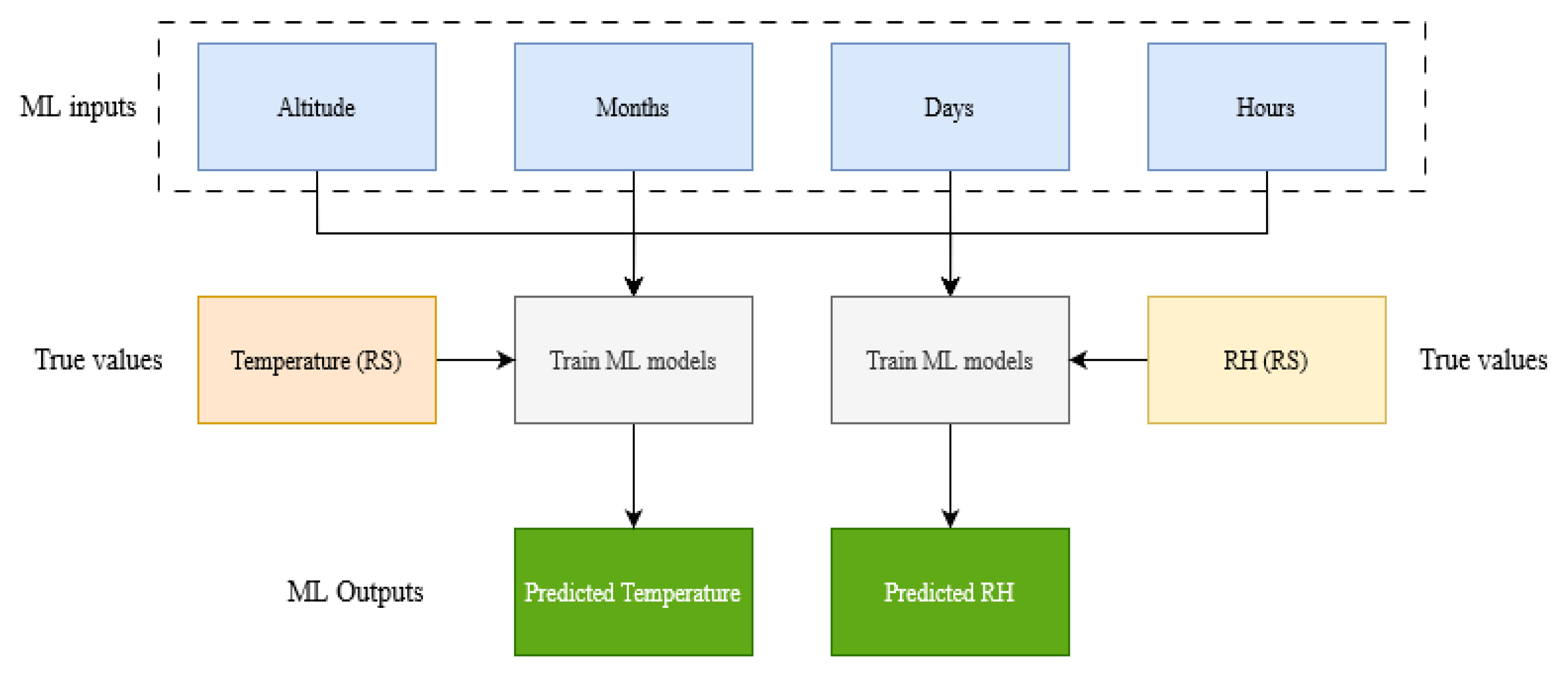
2.1. Overview of Approach and Processing Flow

This study presents a comprehensive methodology for improving the estimation of Cloud Liquid Water Content (CLWC) profiles using machine learning (ML) techniques. The approach integrates high-quality atmospheric datasets, advanced preprocessing techniques, and diverse ML models to achieve accurate predictions. The processing flow is designed to ensure reliability, robustness, and applicability across varying atmospheric conditions.

The ERA5 dataset from the European Centre for Medium-Range Weather Forecasts (ECMWF) served as the primary source of atmospheric data in this study. This dataset provides global coverage with high temporal and spatial resolution, including critical parameters such as temperature, pressure, relative humidity, and specific humidity. Radiosonde observations from the Hong Kong Observatory (HKO) were used as ground truth to validate ERA5 data. The study focuses on ensuring that ERA5 accurately represents real atmospheric conditions, particularly for the unique microclimates in Hong Kong.

To address the significant temporal and spatial discrepancies between ERA5 and radiosonde datasets, a machine learning-based interpolation process was developed and applied to the radiosonde data. Decision tree models were trained to predict radiosonde temperature and relative humidity values for any given altitude and time. Once trained, these models were used to estimate temperature and humidity at the precise altitudes, dates, and times of the ERA5 dataset. This alignment allowed for a fair and rigorous validation of ERA5 data against radiosonde observations, resulting in an excellent correlation between the interpolated radiosonde data and ERA5 measurements. This validation provided confidence in using the ERA5 dataset as the primary dataset for training ML models in CLWC profile prediction.

The preprocessing pipeline addressed ERA5 data quality issues through advanced techniques. Outliers and anomalies were corrected using a hybrid optimization algorithm that combined Antlion Optimization (ALO) and Grasshopper Optimization (GOA). This method improved the correlations between input features (temperature, pressure, relative humidity, and specific humidity) and CLWC profiles, ensuring the dataset’s reliability for ML training. To eliminate short-term fluctuations while preserving meaningful atmospheric trends, three smoothing techniques were applied and compared: moving average (movmean), Gaussian smoothing, and moving median (movmedian).

The processed data were used to train and evaluate a range of ML models, including decision trees, ensemble models (Bagged and Boosted Trees), and neural networks. These models were assessed using robust performance metrics, such as root mean square error (RMSE), mean absolute error (MAE), correlation coefficient, and R-squared (R²). Ensemble models, particularly Bagged Trees, consistently outperformed other approaches, demonstrating superior accuracy and robustness in predicting CLWC.

Figure 1 illustrates the complete processing flow, from data acquisition and validation to preprocessing and model training. This structured approach ensures that the study’s findings are grounded in high-quality data and rigorous analysis, contributing valuable insights to the field of atmospheric science [31].

2.2. Data Description and Analysis

2.2.1. ERA5 Data

The ERA5 dataset from the ECMWF offers full atmospheric coverage from pole to equator [32]. Its temporal resolution is achieved through hourly updates of various factors relating to the atmosphere, land, and seas. This resolution is beneficial for observing the intricate nature of weather systems and detecting subtle climate change variations [33,34]. Regarding spatial resolution, ERA5 datasets cover about 31 km horizontally and 37 vertical levels up to an altitude of 80 km. The data are distributed on a 0.25° × 0.25° grid. ERA5 includes a 10-member ensemble to enhance its robustness, offering insights into the reanalysis’s uncertainty, both temporally and geographically [34]. Our study focuses on the Hong Kong region for the year 2021. The ERA5 data selected for this study encompass the exact latitude and longitude coordinates forming a targeted grid over the area at the following coordinates: 113.49°E–22.33°N, 113.74°E–22.33°N, 113.99°E–22.33°N, 114.24°E–22.33°N, 113.49°E–22.08°N, 113.74°E–22.08°N, 113.99°E–22.08°N, 114.24°E–22.08°N. This investigation spanned a range of atmospheric parameters at 37 different pressure levels, encompassing temperature profiles, relative and specific humidity levels, and cloud liquid water content profiles derived using the ideal gas law and specific cloud liquid water content profiles.

2.2.2. Radiosonde Data

Radiosonde data from the Hong Kong Observatory (HKO) served as the ground truth to validate the integrity of the ERA5 dataset. HKO routinely launches Vaisala RS41-SG radiosondes, which can use both manual and automatic launch processes and collect atmospheric measurements [35]. The radiosondes carefully capture temperature, relative humidity, and pressure observations, with accuracy ranging from 2% to 4%. These observations are obtained every twelve hours, with each sample consisting of around 2331 measurements taken from 66 m up to 30,215 m above ground level. In addition to the primary observations, the radiosondes provide additional data such as wind direction, dew point, and wind speed, which help understand the atmospheric profile up to about 24 km above ground level [35]. These radiosonde data have been used in this study just to prove the validity of the ERA5 data, as mentioned and detailed in Section 2.4.1.

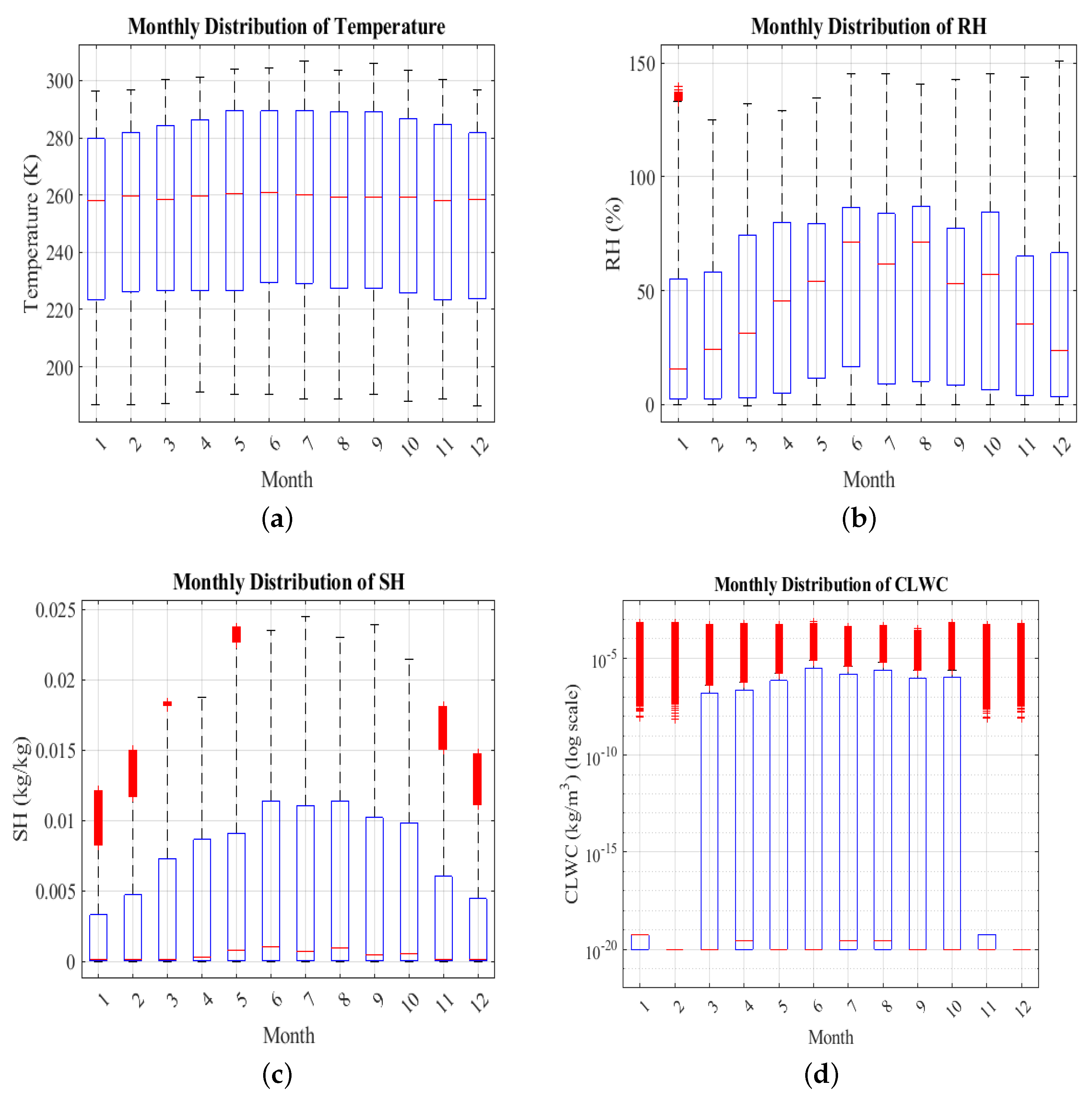
2.3. Climatology of Hong Kong Area and Data Groups

Hong Kong’s subtropical climate exhibits significant seasonal variability that influences Cloud Liquid Water Content (CLWC) values. Winter months (January and February) are characterized by cool and dry conditions with minimal cloud formation and low atmospheric moisture. In spring (March and April), rising temperatures and humidity promote moderate cloud formation and increasing CLWC variability. During summer (May to August), high temperatures, elevated humidity, and frequent thunderstorms lead to peak CLWC values, particularly during the typhoon season from July to September. Autumn (September and October) marks a transition with stabilizing atmospheric conditions and moderate CLWC levels, while late autumn and early winter (November and December) bring cooler, dry, and stable conditions with reduced CLWC variability [36]. Figure 2 illustrates monthly distributions of temperature, relative humidity, specific humidity, and CLWC values for 2021.

To better understand and analyze the impact of these climatological patterns on atmospheric processes, data from 2021 were categorized into five climatological groups as follows: January and February form Group 1, characterized by cooler, drier conditions. Group 2 includes March and April, marking the start of warmer weather and increasing humidity, signaling spring. Group 3, from May to August, represents the summer peak with the highest moisture and temperatures. Group 4, comprising September and October, reflects the transition from peak summer. Finally, Group 5, with November and December, indicates the onset of cooler, drier winter weather. These groups reflect the seasonal characteristics of Hong Kong, capturing the variability of key meteorological parameters, including temperature, relative humidity, specific humidity, and CLWC. This grouping provides a structured approach to studying the region’s unique atmospheric dynamics and their influence on CLWC distribution throughout the year.

2.4. Detailed Methodology

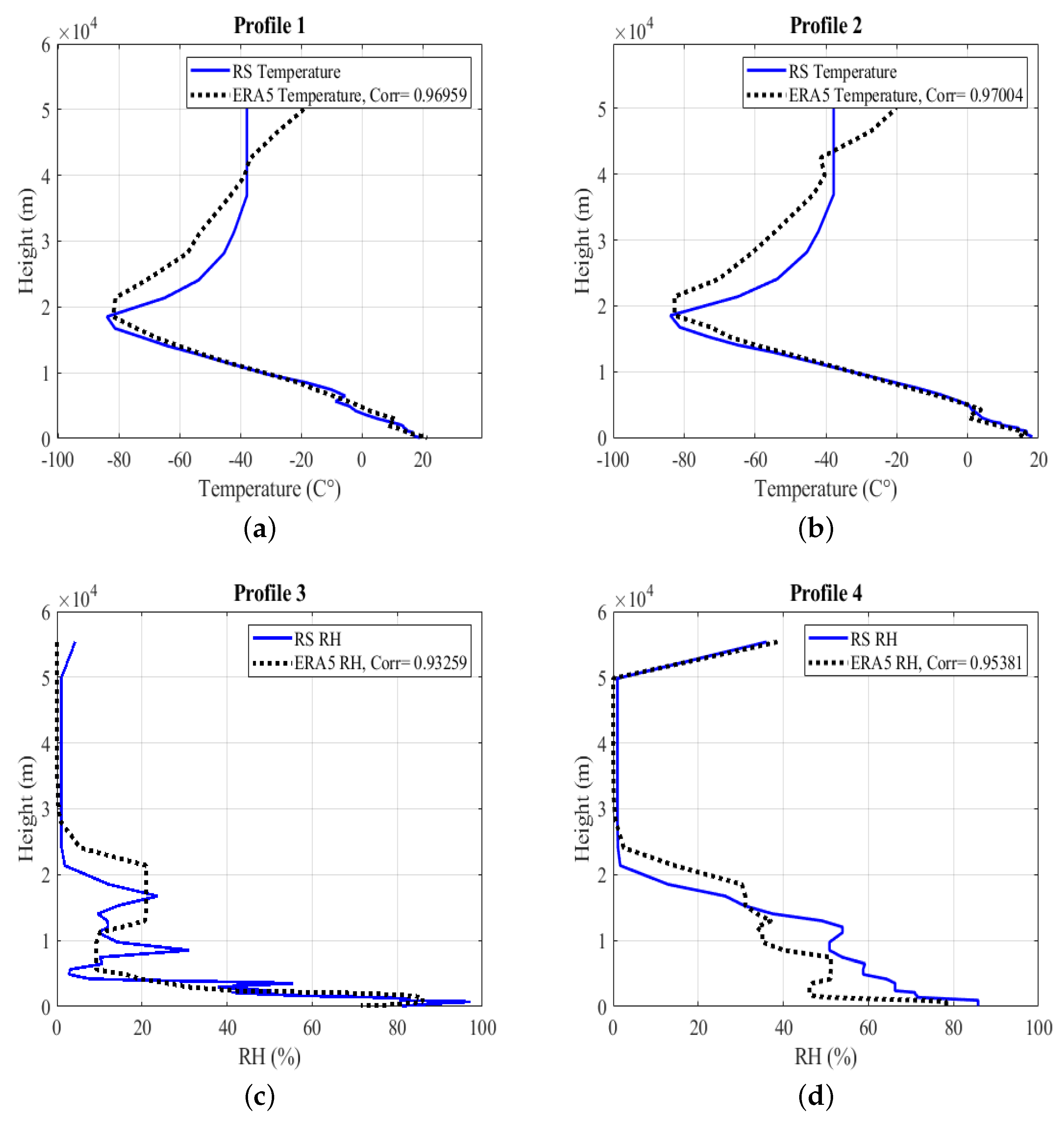
2.4.1. Correlation Between ERA5 and Radiosonde Data

To validate the reliability of the ERA5 dataset for Cloud Liquid Water Content (CLWC) prediction, this study compared ERA5 atmospheric measurements with high-accuracy radiosonde observations from the Hong Kong Observatory (HKO). Radiosonde observations provide precise measurements of atmospheric parameters, including temperature, relative humidity, and pressure. However, significant discrepancies in sampling times and altitudes between the two datasets posed challenges for direct comparison.

To address this issue, machine learning (ML) techniques were employed to interpolate radiosonde values at unsampled altitudes and times (0 and 12 UTC). Figure 3 presents a flow chart of the interpolation framework for temperature and relative humidity using two separate ML models. Both models take altitude, month, day, and hour as input features. The first model outputs interpolated radiosonde temperature values, while the second estimates relative humidity. Fine Tree regression models with a minimum leaf size of 4 were used for both tasks. A total of 958,617 samples were used, split into 85% for training and 15% for testing. Five-fold crossvalidation was applied to enhance model generalizability and robustness.

The performance of the trained models is presented in

Table 1. The performance of machine learning models in predicting the temperature and relative humidity for the radiosonde data in the testing dataset.

Model Type	RMSE	MSE	R-Squared	MAE	Correlation Coefficient
Fine Tree (Temperature (°C))	1.3007	1.6917	0.9984	1.0164	0.9992
Fine Tree (Relative humidity (%))	3.0501	9.3032	0.9894	1.8300	0.9965

. The temperature interpolation model achieved an R-squared value of 0.9984 and a correlation coefficient of 0.9992 on the testing dataset, along with low error values (RMSE = 1.3007 °C; MAE = 1.0164 °C). The relative humidity model also demonstrated strong predictive performance, with an R-squared of 0.9894 and a correlation coefficient of 0.9965 (RMSE = 3.0501%; MAE = 1.8300%). These results confirm the effectiveness of the ML models in generating accurate interpolated profiles.

Figure 4 compares ML-interpolated and actual radiosonde profiles for relative humidity and temperature. The fine decision tree showed high accuracy, closely matching real data. As seen in (a), it captured humidity variation with altitude; as seen in (b), it accurately reproduced temperature changes. The model achieved correlation coefficients of 0.9953 for humidity and 0.9942 for temperature, confirming its strong predictive performance.

Based on these results, the interpolated radiosonde temperature and relative humidity values were used to align the radiosonde and ERA5 datasets at common time and height points. This generated a matched dataset for robust comparison across both data sources. This interpolation process was completed prior to training the CLWC prediction models to ensure consistent and aligned inputs for machine learning. It is important to note that the radiosonde data were used solely for validating the reliability of ERA5 temperature and relative humidity. They were not used in the cleaning or optimization stages of the modeling pipeline. All subsequent data cleaning, feature optimization, and CLWC prediction steps were conducted entirely within the ERA5 dataset. This approach ensured internal consistency among the input and target variables while leveraging radiosonde observations only for independent input validation.

Subsequently, correlation coefficients were calculated between the interpolated radiosonde values and ERA5 data for temperature and relative humidity from January to June 2021, as summarized in

Table 2. Correlation coefficients between ERA5 and radiosonde measurements.

	Temperature Correlation	Relative Humidity Correlation
January	0.9486	0.7435
February	0.9570	0.7495
March	0.9683	0.7697
April	0.9686	0.7404
May	0.9686	0.7976
June	0.9667	0.8159
All six months	0.9632	0.7808

. The average correlation coefficient for relative humidity across all months was 0.7808, with monthly values ranging from 0.7404 to 0.8159. Temperature correlations were consistently higher, with an average of 0.9632 and values ranging from 0.9486 in January to 0.9667 in June. These findings indicate a strong agreement between the two datasets. Only the first six months are included due to data availability from the Hong Kong Observatory.

To further validate the ERA5 dataset, Figure 5 presents height profiles comparing ERA5 values with interpolated radiosonde values. Subfigures (a) and (b) display temperature profiles for two representative cases, yielding correlation coefficients of 0.9696 and 0.9700, respectively. Subfigures (c) and (d) show the corresponding relative humidity profiles, which also reveal strong agreement, with correlation values of 0.9538 and 0.9326. These results demonstrate consistent alignment between the two sources across different atmospheric levels despite natural variability in humidity.

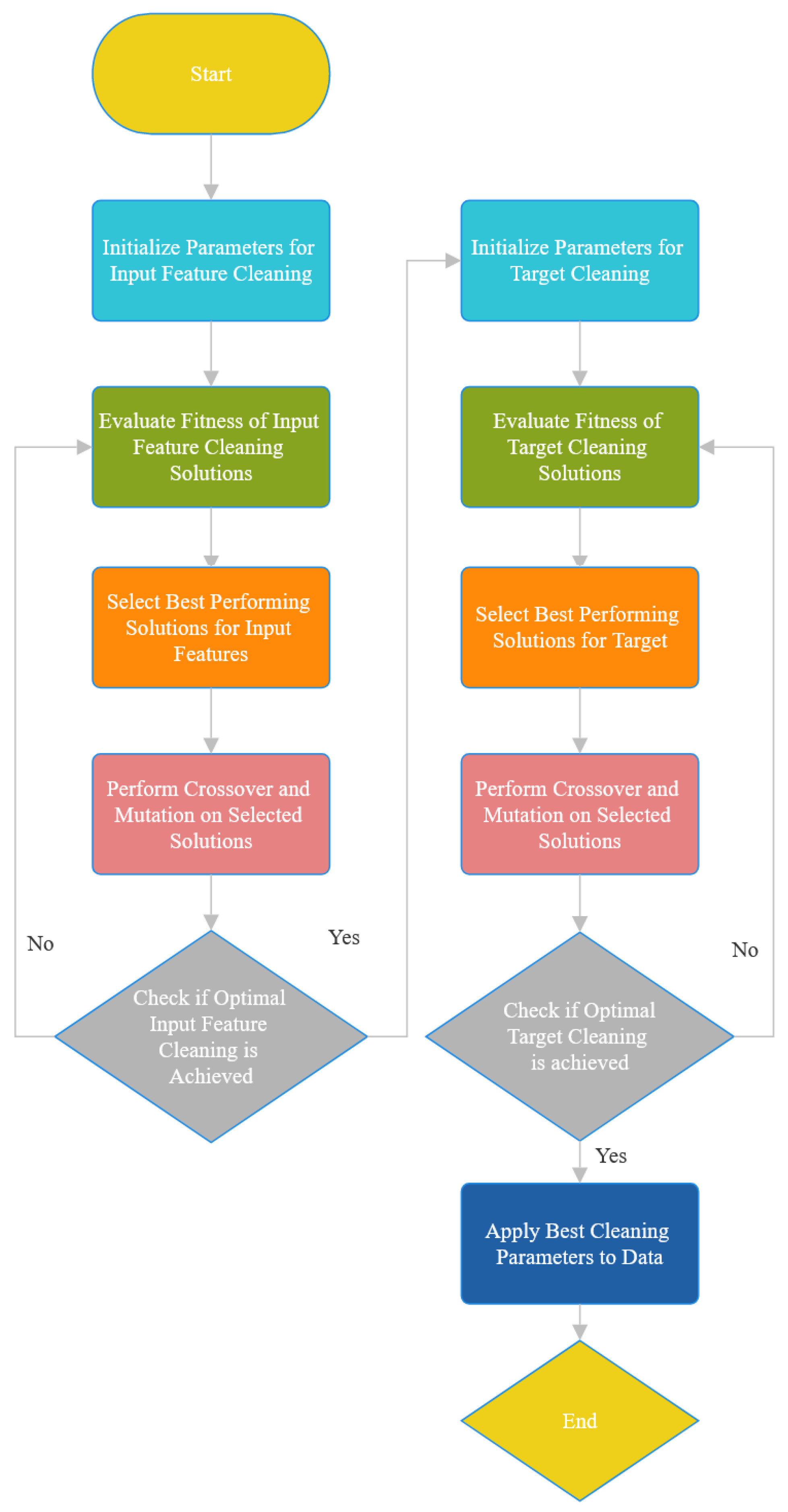
2.4.2. Data Quality Control and Prepossessing

Ensuring high data quality is critical for improving the accuracy and reliability of Cloud Liquid Water Content (CLWC) predictions, particularly given the variability and noise inherent in atmospheric datasets. This study employed a comprehensive preprocessing pipeline to address data anomalies, optimize features’ correlations, and prepare the dataset for machine learning (ML) analysis. The pipeline included advanced data cleaning and smoothing, using optimization techniques tailored to the specific challenges of atmospheric data.

Outliers, which can significantly distort predictions, were identified and corrected. These anomalies often arise from environmental factors or sensor malfunctions during critical data collection periods. To systematically clean the dataset, a hybrid optimization algorithm combining Antlion Optimization (ALO) and Grasshopper Optimization Algorithm (GOA) was implemented [37,38]. This approach leverages the strengths of both algorithms by balancing exploration (the ability to broadly search the solution space for diverse potential solutions) and exploitation (the focused refinement of high-quality solutions to converge on optimal data-cleaning parameters). This balance enhances the robustness of the preprocessing process, particularly in complex atmospheric datasets where noise and variability are common.

As part of the hybrid optimization algorithm, a fitness function, serving as the objective function, is formulated to guide the preprocessing process. This fitness score quantifies the quality of each data-cleaning solution based on the correlation between the cleaned input feature and the target CLWC. The function is defined as follows:

$$fitness=min\left({\displaystyle \frac{1}{\left|\mathrm{corr}(cleane{d}_{i}npu{t}_{f}eature,Outpu{t}_{t}arget)\right|}}\right)$$

(1)

This objective function was applied independently to each input feature (temperature, pressure, relative humidity, and specific humidity), allowing the optimization algorithm to separately maximize the correlation between inputs and the output.

The preprocessing steps were guided by this objective function and iteratively refined using the hybrid algorithm. Outlier correction and smoothing were implemented to ensure robust alignment between input features and CLWC values. The results of this preprocessing demonstrated significant improvements in data quality. Correlation coefficients between input features and CLWC increased substantially. For instance, the correlation between pressure and CLWC improved from 0.21 to 0.68, while the correlation between ERA5 temperature and CLWC increased from 0.20 to 0.69 after applying the cleaning and optimization process. Similar enhancements were observed for relative humidity and specific humidity, with correlations increasing by over 50%. These results underscore the effectiveness of the hybrid optimization algorithm in enhancing dataset reliability and ensuring robust predictions.

Figure 6 illustrates the complete preprocessing pipeline based on a hybrid metaheuristic optimization strategy. The left-hand branch focuses on cleaning the input features—namely, temperature, pressure, relative humidity, and specific humidity—while the right-hand branch targets the cleaning of the output variable—Cloud Liquid Water Content (CLWC). Each side begins with parameter initialization, followed by an evaluation of solution fitness based on correlation with the prediction target (for inputs) or input alignment (for the target). Best-performing solutions are selected and undergo crossover and mutation steps inspired by evolutionary algorithms. These steps are repeated iteratively until the optimal data-cleaning configuration is achieved. Although both sides of the figure follow an identical optimization cycle, they serve distinct roles: the input cleaning stream aims to enhance signal relevance and remove noise that may reduce model generalizability, while the target cleaning stream ensures that the CLWC values themselves are free from irregular spikes or anomalies that would bias training. Performing the same process separately allows for targeted adaptation, which would not be possible in a unified cleaning pipeline. To the best of our knowledge, this dual-track hybrid optimization for independently preprocessing both input and target variables has not been previously reported in the atmospheric or remote sensing literature. Existing studies often focus only on feature-side cleaning. The novelty of our approach lies in optimizing both ends of the machine learning pipeline using metaheuristic evolution strategies, which enhances model robustness and improves correlation significantly.

By systematically addressing data inconsistencies, this methodology ensured that the final dataset was well suited for training robust ML models capable of accurate CLWC predictions.

2.4.3. Performance Evaluation Metrics for CLWC Estimation

Evaluating algorithm performance in predicting Cloud Liquid Water Content values involves several statistical metrics, each offering unique insights into the algorithms’ prediction performance. Mean absolute error (MAE) is the first of these metrics represented through the equation:

$$MAE={\displaystyle \frac{1}{N}}\sum _{i=1}^N\left|X_{true}\left(i\right)-X_{predicted}\left(i\right)\right|$$

(2)

where N represents the total count of data samples, while $X_{true}$ and $X_{predicted}$ denote the actual observed values and the values predicted by the model, respectively. MAE measures the average magnitude of prediction errors by calculating the mean of the absolute differences between actual and forecasted observations. This metric is especially valuable in scenarios where errors are weighed proportionally to their absolute magnitude, making it less sensitive to large outliers than RMSE [39].

Secondly, the root mean square error (RMSE) provides a more detailed assessment of prediction accuracy:

$$RMSE=\sqrt{\left[\left(\sum _{i=1}^N{\left(X_{true}\left(i\right)-X_{predicted}\left(i\right)\right)}^2\right)/N\right]}$$

(3)

RMSE is particularly sensitive to more significant errors due to its squaring of the differences before averaging. This sensitivity makes RMSE invaluable when significant errors are more detrimental than smaller ones. However, its interpretation can be less intuitive than MAE due to the squaring and square root steps, even though RMSE retains the same units as the original data [35].

Another critical metric is the mean squared error (MSE), which is given by

$$MSE={\displaystyle \frac{1}{N}}\sum _{i=1}^N{\left(X_{true}\left(i\right)-X_{predicted}\left(i\right)\right)}^2$$

(4)

Like RMSE, MSE emphasizes more significant errors by squaring the differences between true and predicted values. This feature makes MSE a key metric in contexts where more significant deviations need to be penalized more heavily. MSE is also preferred for its mathematical properties in optimization contexts. However, unlike RMSE, MSE has squared units, which can make its interpretation less intuitive when evaluating model errors [35].

The correlation coefficient $\left(\rho \right)$ shifts the focus from error magnitude to the linear relationship between actual and predicted values. It is calculated using the following formula:

$$\begin{array}{c}\hfill \rho \left(X_{true},X_{predicted}\right)={\displaystyle \frac{1}{N-1}}\sum _{i=1}^N\left({\displaystyle \frac{X_{true}\left(i\right)-{\mu }_{true}}{{\sigma }_{true}}}\right)\\ \hfill \left({\displaystyle \frac{X_{predicted}\left(i\right)-{\mu }_{predicted}}{{\sigma }_{predicted}}}\right)\end{array}$$

(5)

In Equation (5), $\mu$ represents the mean, and $\sigma$ stands for the standard deviation. This coefficient ranges from −1 to 1, providing insight into how closely the changes in predicted values correspond to changes in actual values. While the correlation coefficient effectively measures the strength of the linear relationship between predicted and actual values, it does not reflect the magnitude of individual errors. Therefore, it is best interpreted alongside error-based metrics such as RMSE or MAE for a complete assessment of predictive performance [35].

Finally, the coefficient of determination (R-squared or $R^2)$ offers a different perspective on model performance. It is represented by

$$R^2=1-{\displaystyle \frac{{\sum }_{i=1}^N{\left(X_{true}\left(i\right)-X_{predicted}\left(i\right)\right)}^2}{{\sum }_{i=1}^N{\left(X_{true}\left(i\right)-\overline{X_{true}}\right)}^2}}$$

(6)

R-squared quantifies the proportion of variance in the dependent variable that is predictable from the independent variables. This metric is instrumental in regression problems, as it measures how much of the variability in the outcome can be explained by the model, offering insights into the effectiveness of the independent variables in predicting the dependent variable. A higher R-squared value is often sought after, as it indicates that a greater proportion of variance in the dependent variable is accounted for by the model, suggesting a stronger predictive ability in the context of the regression analysis [40].

2.4.4. ML Algorithms and Methods Used in This Study

This study employed diverse machine learning (ML) algorithms to predict Cloud Liquid Water Content (CLWC), with each selected for its unique strengths in handling nonlinear relationships and complex atmospheric data. The models include decision trees, ensemble trees, and neural networks, which were tailored to the characteristics of the dataset.

Decision tree models were utilized for their interpretability and ability to capture nonlinear patterns. These models are particularly effective in atmospheric studies where relationships between variables can be complex. Ensemble methods were implemented to enhance accuracy by reducing variance and improving generalization [35].

Neural networks were applied to explore their capacity for modeling complex, high-dimensional data. While these models offer flexibility in learning intricate patterns, their performance is sensitive to network depth and neuron configurations, requiring careful tuning to avoid overfitting [35].

Each model was trained and evaluated using the preprocessed ERA5 dataset described earlier. The dataset was divided into training (85%) and testing (15%) subsets, with five-fold crossvalidation applied to ensure robustness and minimize overfitting. Performance metrics, including RMSE, MAE, and R-squared, were used to evaluate the models, as detailed in the evaluation metrics section.

Table A1. Overview of machine learning models and their hyperparameters.

Model Type	Hyperparameters
Linear Regression (LR)	Linear term only
Fine Tree (FT)	Minimum leaf size: 4
Bagged Ensemble Tree (BTT)	Minimum leaf size: 8; Number of learners: 30
Wide Neural Network (WNN)	Single layer with 100 neurons; Activation function: ReLU; Iteration limit: 1000
Trilayered Neural Network (TriNN)	Three layers, each with 10 neurons; Activation function: ReLU; Iteration limit: 1000

summarizes the models’ configurations, including key parameters such as tree leaf size, number of learners, and neural network layers. For example, the Fine Tree model utilized a minimum leaf size of 4, while Bagged Trees included 30 learners. This table is provided in the Appendix A for reference.

3. Results

This section describes the results of using various machine learning algorithms to predict Cloud Liquid Water Content profiles. The study utilized meteorological data from Hong Kong for the year 2021. This dataset (containing 2,592,950 samples) originated from ERA5 data gathered across eight specific locations in Hong Kong and was analyzed at 37 atmospheric pressure levels throughout the year. It was then organized into one comprehensive dataset for the entire year, as well as five distinct groups based on the specific meteorological characteristics described earlier. For the analysis, the data were partitioned into two distinct subsets: 85% was employed for a detailed crossvalidation process, utilizing a k = 5-fold method for thorough training and validation, while the remaining 15% was reserved for testing the models’ performance.

To mitigate overfitting, the K-fold crossvalidation technique and early stopping were implemented. The former divides the data into five subsets, each used once as validation data, offering a reliable performance estimate on unseen data. On the other hand, early stopping monitors the model’s performance during training and stops the process if the validation error increases. This combination of techniques effectively balances bias and variance, limiting overfitting and ensuring accurate model performance evaluation. The first subsection of this analysis focuses on the outcomes of applying these algorithms to the full-year dataset. This includes a detailed examination of performance metrics and insights gained from the crossvalidation process. The second subsection shifts to analyzing the grouped data, adhering to the previously described categorization process.

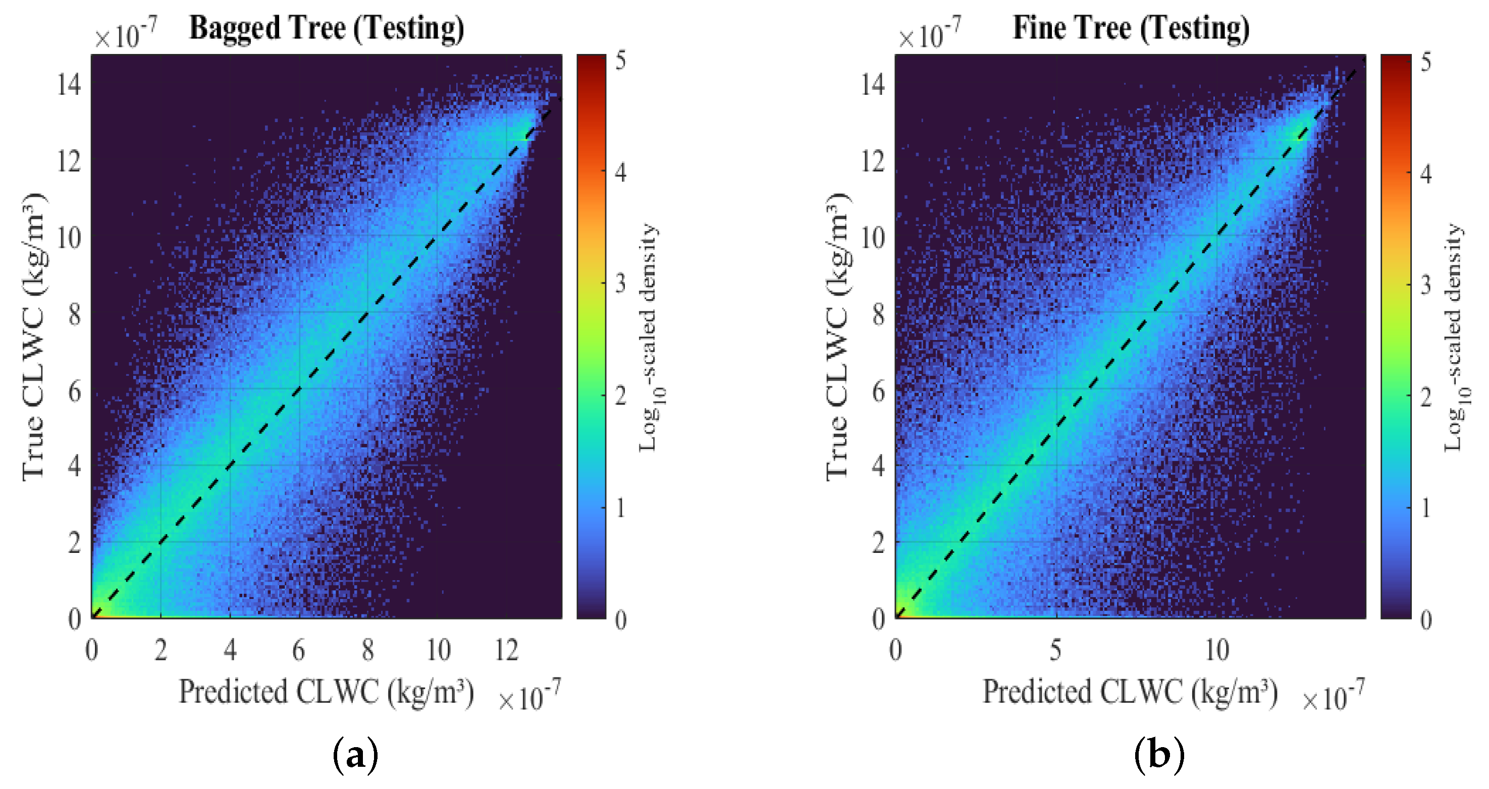
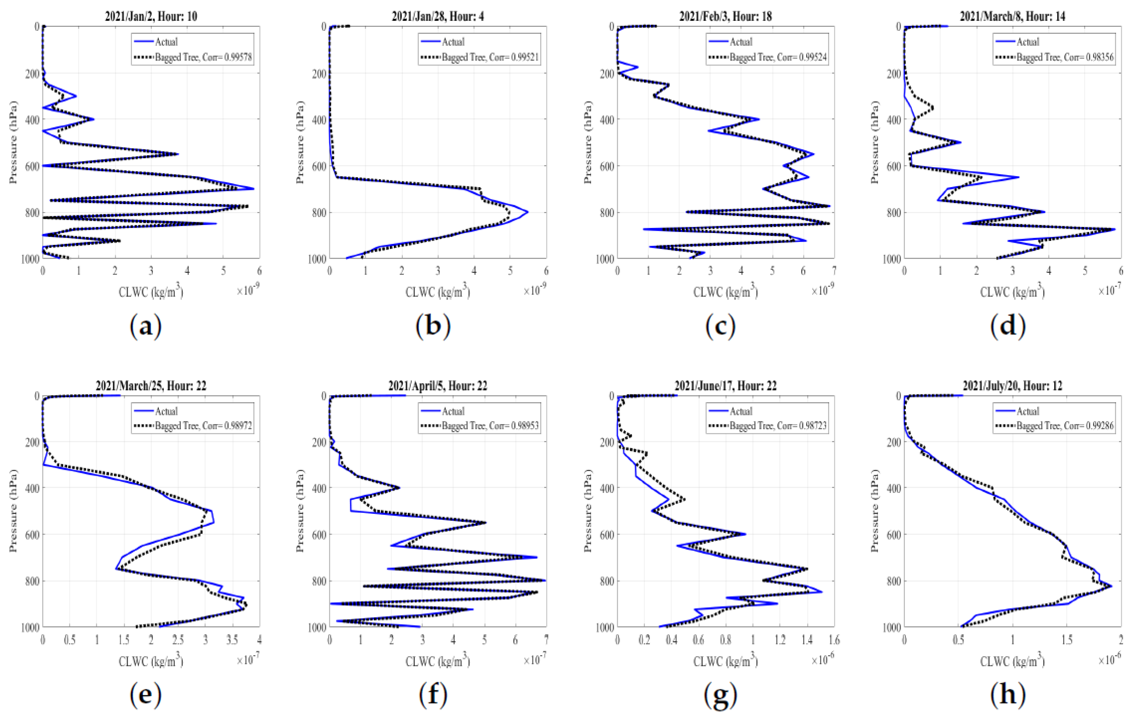
3.1. Analysis of Results Based on the Full-Year Data

Table 3. Performance results of various machine learning models for predicting Cloud Liquid Water Content (CLWC) in the 2021 training dataset.

Model Type	RMSE (kg/m3)	MSE (kg/m3)2	R2	MAE (kg/m3)	Correlation
Fine Tree	$1.41\times {10}^{-7}$	$1.98\times {10}^{-14}$	0.85895	$7.56\times {10}^{-8}$	0.9736
Bagged Tree	$1.25\times {10}^{-7}$	$1.57\times {10}^{-14}$	0.88800	$7.42\times {10}^{-8}$	0.9678
WNN	$9.99\times {10}^{-4}$	$9.97\times {10}^{-7}$	$-7109489$	$6.00\times {10}^{-4}$	0.0112
TriNN	$9.16\times {10}^{-4}$	$8.39\times {10}^{-7}$	$-5982461$	$5.00\times {10}^{-4}$	0.0198
LR	$2.16\times {10}^{-7}$	$4.66\times {10}^{-14}$	0.667978	$1.60\times {10}^{-7}$	0.8173

summarizes the performance of various machine learning models for predicting Cloud Liquid Water Content (CLWC) values using the 2021 training dataset, while

Table 4. Performance results of various machine learning models for predicting Cloud Liquid Water Content (CLWC) in the 2021 testing dataset.

Model Type	MAE (kg/m3)	MSE (kg/m3)2	RMSE (kg/m3)	R2	Correlation
Fine Tree	$7.26\times {10}^{-8}$	$1.84\times {10}^{-14}$	$1.36\times {10}^{-7}$	0.8692	0.9331
Bagged Tree	$7.26\times {10}^{-8}$	$1.50\times {10}^{-14}$	$1.23\times {10}^{-7}$	0.8932	0.9452
WNN	$6.20\times {10}^{-4}$	$1.00\times {10}^{-6}$	$1.00\times {10}^{-3}$	$-7.117\times {10}^6$	0.0127
TriNN	$6.40\times {10}^{-4}$	$9.84\times {10}^{-7}$	$9.90\times {10}^{-4}$	$-6.998\times {10}^6$	0.0227
LR	$1.60\times {10}^{-7}$	$4.67\times {10}^{-14}$	$2.16\times {10}^{-7}$	0.6675	0.817

presents their performance on the testing dataset. The testing dataset results validate the trends observed during training, with Bagged Tree consistently emerging as the top-performing model.It achieved the lowest RMSE ($1.23\times {10}^{-7}$ kg/m³) and MSE ($1.50\times {10}^{-14}$ (kg/m³)²), along with the highest R-squared value (0.8932) and correlation coefficient (0.9452). These results reinforce its robustness and generalizability across unseen data.

Similarly, the Fine Tree model maintained strong performance in the testing dataset, achieving an RMSE of $1.36\times {10}^{-7}$ kg/m³ and an R-squared value of 0.8692. This further confirms its reliability in capturing the nonlinear relationships inherent in the dataset. In contrast, the neural network models (WNN and TriNN) continued to exhibit poor performance, with significantly higher RMSE values ($1.0\times {10}^{-3}$ and $9.9\times {10}^{-4}$ kg/m³, respectively) and large negative R-squared scores. As observed in the training dataset, the ReLU activation function’s inability to prevent "dead neurons" and the networks’ simplistic architectures limited their capacity to generalize to the testing data.

The linear regression (LR) model showed better results than neural networks but remained weaker than the tree-based models, with an RMSE of $2.16\times {10}^{-7}$ kg/m³ and an R-squared value of 0.6675. This further highlights the limitations of linear models in handling the complex dynamics of atmospheric data. These extreme R² values are mathematically valid and occur when the model errors greatly exceed the variance of the ground truth, which confirms total model failure in those cases.

The consistent superior performance of tree-based models, particularly Bagged Trees, across both training and testing datasets, emphasizes their effectiveness in CLWC prediction. However, the neural networks and linear regression model faced challenges in capturing the intricate nonlinearities of the dataset, underscoring the need for robust algorithms tailored to the complexities of atmospheric data.

Figure 7 and Figure 8 present scatter density plots that provide a comprehensive visual narrative of multiple machine learning models’ effectiveness in predicting CLWC profiles across training and testing datasets.

The Bagged Tree and Fine Tree models resulted in good accuracy in the training dataset analysis, as shown in Figure 7. Their scatter plots are characterized by densely packed dots along the diagonal, suggesting that most predictions closely match the actual measurements. The Bagged Tree, in particular, has a tighter cluster of data points, suggesting its somewhat higher accuracy.

The scatter density plots for the testing dataset, as shown in Figure 8, present the tested and verified performances of the ML algorithms. The Bagged Tree model provided accurate predictions that closely match actual responses, producing a dense cluster along the center line, which supports the high R-squared and correlation coefficient values. Although the Fine Tree model produced a slightly more distributed scatter of points, it still yielded good prediction accuracy.

The group of profiles presented in Figure 9 offers a comparative visualization of CLWC predictions from three distinct machine learning models (Bagged Trees, Fine Tree, and linear regression) against actual measured values from radiosondes across varying pressure levels. These profiles were selected randomly at various times and under different environmental conditions. The y axis in each subfigure has been reversed to represent the actual altitudes intuitively.

These sample profiles demonstrate that the Bagged Trees and Fine Tree models closely follow the actual CLWC values across the pressure levels. This consistency is particularly evident in profiles like a, b, d, and e, where the correlation coefficients are very high, suggesting high prediction accuracy. In contrast, the linear regression model, while generally matching the trend of actual CLWC values, tended to diverge at specific pressure levels. For instance, profiles b, e, and g show scenarios where the linear regression predictions differ significantly from the real observations at nearly all pressure levels, resulting in the lowest correlation coefficients. This divergence highlights the model’s limitations in adapting to the nonlinear nature of atmospheric data, as linear techniques may not adequately capture the dynamics of cloud formation.

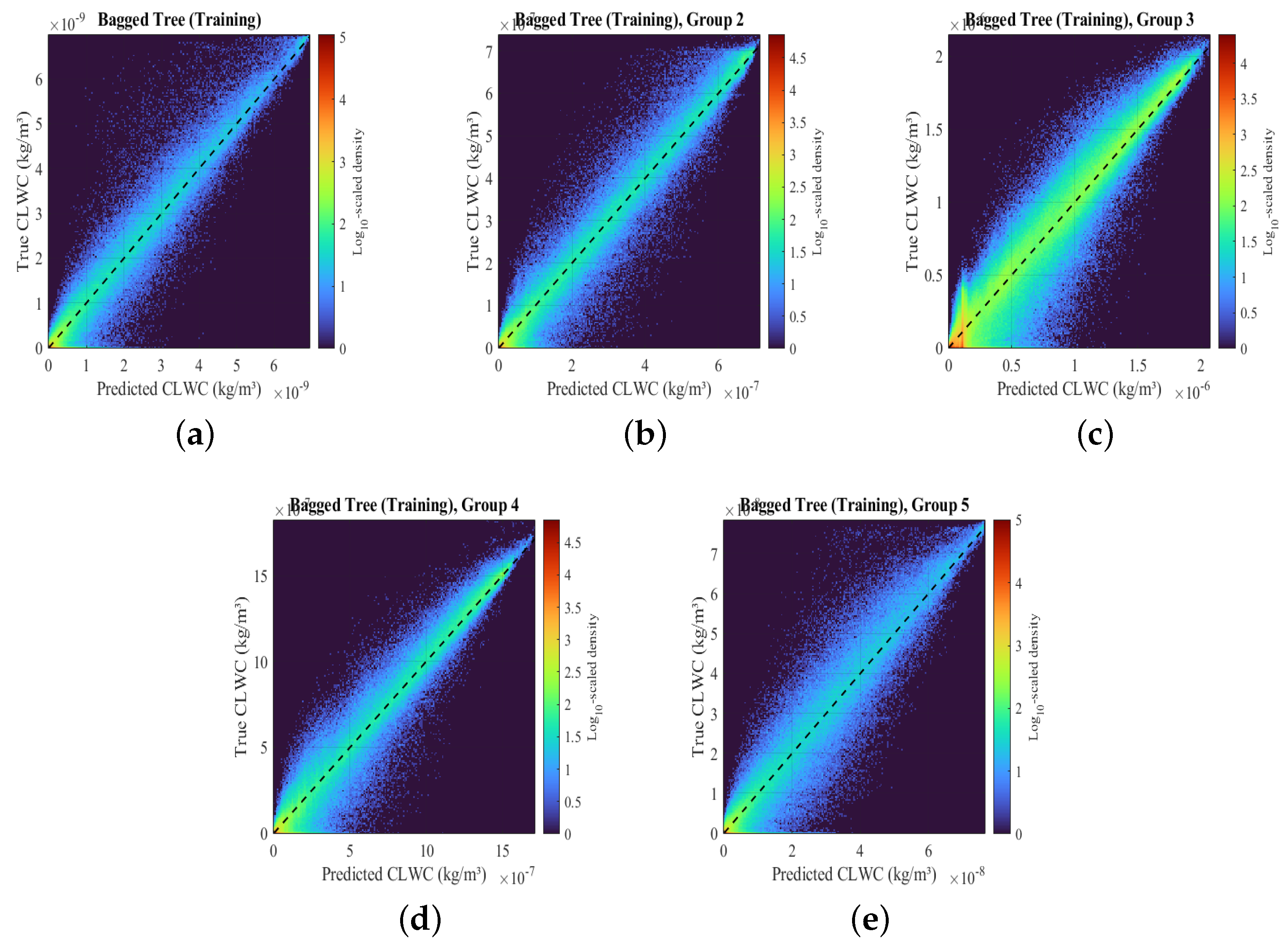
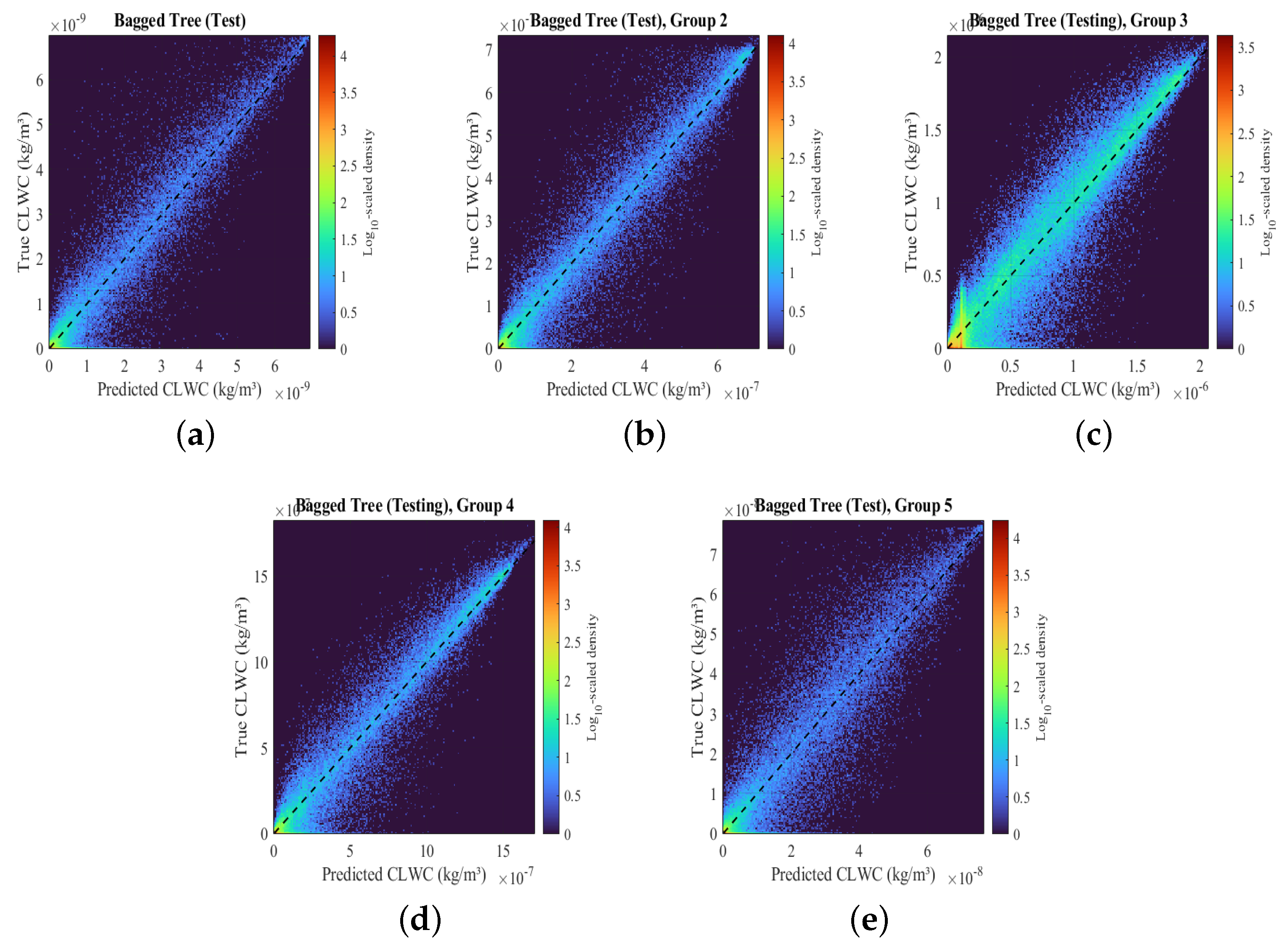
3.2. Performance Evaluations Based on Grouped Datasets

Table 5. Performance results of machine learning models across different groups in the 2021 training dataset for CLWC prediction.

Model Type	RMSE (kg/m3)	MSE (kg/m3)2	R2	MAE (kg/m3)	Correlation
Group 1 Bagged Tree	$4.55\times {10}^{-10}$	$2.07\times {10}^{-19}$	0.9214	$2.46\times {10}^{-10}$	0.9602
Group 1 Fine Tree	$5.09\times {10}^{-10}$	$2.59\times {10}^{-19}$	0.9018	$2.32\times {10}^{-10}$	0.9502
Group 1 WNN	$1.00\times {10}^{-3}$	$1.00\times {10}^{-6}$	$-3.8\times {10}^{11}$	$7.00\times {10}^{-4}$	$-0.0061$
Group 2 Bagged Tree	$5.05\times {10}^{-8}$	$2.55\times {10}^{-15}$	0.9431	$2.94\times {10}^{-8}$	0.9713
Group 2 Fine Tree	$5.69\times {10}^{-8}$	$3.24\times {10}^{-15}$	0.9276	$2.89\times {10}^{-8}$	0.9634
Group 2 WNN	$1.00\times {10}^{-3}$	$1.00\times {10}^{-6}$	$-2.2\times {10}^7$	$6.00\times {10}^{-4}$	0.0011
Group 3 Bagged Tree	$1.71\times {10}^{-7}$	$2.92\times {10}^{-14}$	0.9143	$1.15\times {10}^{-7}$	0.9564
Group 3 Fine Tree	$1.74\times {10}^{-7}$	$3.04\times {10}^{-14}$	0.9105	$1.03\times {10}^{-7}$	0.9546
Group 3 WNN	$1.00\times {10}^{-3}$	$9.94\times {10}^{-7}$	$-2.92\times {10}^5$	$6.00\times {10}^{-4}$	$-0.0227$
Group 4 Bagged Tree	$1.15\times {10}^{-7}$	$1.32\times {10}^{-14}$	0.9468	$6.82\times {10}^{-8}$	0.9733
Group 4 Fine Tree	$1.26\times {10}^{-7}$	$1.58\times {10}^{-14}$	0.9360	$6.41\times {10}^{-8}$	0.9677
Group 4 WNN	$1.00\times {10}^{-3}$	$1.01\times {10}^{-6}$	$-4.07\times {10}^5$	$6.00\times {10}^{-4}$	0.0093
Group 5 Bagged Tree	$6.21\times {10}^{-9}$	$3.86\times {10}^{-17}$	0.8962	$3.48\times {10}^{-9}$	0.9467
Group 5 Fine Tree	$7.36\times {10}^{-9}$	$5.42\times {10}^{-17}$	0.8543	$3.78\times {10}^{-9}$	0.9257
Group 5 WNN	$1.00\times {10}^{-3}$	$1.02\times {10}^{-6}$	$-2.7\times {10}^9$	$7.00\times {10}^{-4}$	0.0222

presents the performance of machine learning models for predicting Cloud Liquid Water Content (CLWC) across different groups in the 2021 training dataset, while

Table 6. Performance results of machine learning models across different groups in the 2021 testing dataset for CLWC prediction.

Model Type	RMSE (kg/m3)	MSE (kg/m3)2	R2	MAE (kg/m3)	Correlation
Group 1 Bagged Tree	$4.42\times {10}^{-10}$	$1.96\times {10}^{-19}$	0.9257	$2.35\times {10}^{-10}$	0.9624
Group 1 Fine Tree	$4.90\times {10}^{-10}$	$2.40\times {10}^{-19}$	0.9089	$2.16\times {10}^{-10}$	0.9538
Group 1 WNN	$1.00\times {10}^{-3}$	$1.03\times {10}^{-6}$	$-3.9\times {10}^{11}$	$7.00\times {10}^{-4}$	$-0.0107$
Group 2 Bagged Tree	$4.77\times {10}^{-8}$	$2.28\times {10}^{-15}$	0.9493	$2.77\times {10}^{-8}$	0.9745
Group 2 Fine Tree	$5.38\times {10}^{-8}$	$2.90\times {10}^{-15}$	0.9355	$2.68\times {10}^{-8}$	0.9674
Group 2 WNN	$1.00\times {10}^{-3}$	$1.02\times {10}^{-6}$	$-2.3\times {10}^7$	$6.00\times {10}^{-4}$	0.0212
Group 3 Bagged Tree	$1.67\times {10}^{-7}$	$2.77\times {10}^{-14}$	0.9188	$1.11\times {10}^{-7}$	0.9588
Group 3 Fine Tree	$1.67\times {10}^{-7}$	$2.78\times {10}^{-14}$	0.9186	$9.81\times {10}^{-8}$	0.9587
Group 3 WNN	$1.00\times {10}^{-3}$	$9.77\times {10}^{-7}$	$-2.86\times {10}^6$	$6.00\times {10}^{-4}$	$-0.0011$
Group 4 Bagged Tree	$1.10\times {10}^{-7}$	$1.21\times {10}^{-14}$	0.9509	$6.51\times {10}^{-8}$	0.9754
Group 4 Fine Tree	$1.20\times {10}^{-7}$	$1.44\times {10}^{-14}$	0.9416	$6.14\times {10}^{-8}$	0.9706
Group 4 WNN	$1.00\times {10}^{-3}$	$1.00\times {10}^{-6}$	$-4.05\times {10}^6$	$6.00\times {10}^{-4}$	0.0028
Group 5 Bagged Tree	$6.14\times {10}^{-9}$	$3.77\times {10}^{-17}$	0.8988	$3.41\times {10}^{-9}$	0.9481
Group 5 Fine Tree	$7.22\times {10}^{-9}$	$5.21\times {10}^{-17}$	0.8601	$3.69\times {10}^{-9}$	0.9286
Group 5 WNN	$1.00\times {10}^{-3}$	$1.01\times {10}^{-6}$	$-2.7\times {10}^9$	$7.00\times {10}^{-4}$	$-0.0277$

shows their performance on the corresponding testing dataset. These grouped evaluations provide insights into how the models perform under varying atmospheric conditions.

The Bagged Tree model consistently delivered the best performance across all groups in both the training and testing datasets. For instance, in Group 1, it achieved an RMSE of $4.55\times {10}^{-10}$ kg/m³ (training) and $4.42\times {10}^{-10}$ kg/m³ (testing), along with high R-squared values (0.9214 for training and 0.9257 for testing). Similar trends were observed in other groups, with Bagged Trees maintaining superior accuracy and robustness in handling data variability. This highlights the model’s ability to generalize effectively and adapt to different atmospheric patterns.

The Fine Tree model also performed well, though slightly weaker than Bagged Trees. In Group 1, for example, its RMSE was $5.09\times {10}^{-10}$ kg/m³ in the training dataset and $4.89\times {10}^{-10}$ kg/m³ in the testing dataset, with corresponding R-squared values of 0.9018 and 0.9089. These results confirm the reliability of Fine Trees as an alternative when computational efficiency is prioritized.

Conversely, the neural network models (WNN and TriNN) exhibited poor performance across all groups, with significantly higher RMSE values (e.g., $1.00\times {10}^{-3}$ kg/m³) and large negative R-squared scores. These outcomes reinforce the challenges faced by neural networks in this study, including the “dead neuron” issue associated with ReLU activation and its inability to capture the nonlinear dynamics of CLWC data effectively.

The consistently superior performance of tree-based models, particularly Bagged Trees, underscores their robustness in handling grouped data. The results also highlight the importance of selecting models capable of addressing the complexities of atmospheric datasets while ensuring generalizability across different conditions.

Figure 10 and Figure 11 display scatter density plots of predicted versus actual CLWC values for Groups 1 to 5 during the training and testing phases, respectively. Across all groups, the Bagged Tree model demonstrated strong alignment with actual CLWC values, particularly at lower ranges, where the density clusters are tightly concentrated along the diagonal.

In Group 1, the Bagged Tree model achieved high predictive accuracy, as evident in the clear clustering along the diagonal. Similar trends can be observed in Group 2, where the model exhibited consistent predictive symmetry and reduced dispersion. These characteristics were maintained across Groups 3 to 5, further highlighting the robustness of the Bagged Tree model in both the training and testing phases.

The consistency in the patterns of scatter density between the training and testing stages underscores the ability of the model to generalize effectively to unseen data. These results confirm the reliability of the Bagged Tree model in capturing the nonlinear relationships inherent in atmospheric datasets and its suitability for CLWC prediction.

Figure 12 demonstrates the ability of the Bagged Tree model to predict CLWC values in various atmospheric pressures for five distinct climatological groups. The y axis in each subfigure has been reversed to represent the actual altitudes accurately. For each climatological group, the predicted CLWC profiles and the actual CLWC values are presented at different times. The Bagged Tree model consistently aligned its predictions with the actual CLWC profiles across all examples, as evidenced by the high correlation coefficients ranging from 0.983 to 0.996. This indicates the robust performance of the model across all atmospheric pressure levels and its adaptability in varying climatic conditions.

4. Discussion

While this study demonstrates the effectiveness of machine learning models for CLWC estimation, it does not include a direct comparison with traditional physical models, such as radiative transfer-based retrievals or parameterization schemes in numerical weather prediction systems. These conventional approaches often involve assumptions that may limit their accuracy under complex atmospheric conditions. In contrast, our data-driven models offer flexibility in capturing nonlinear relationships from real-world observations. A quantitative comparison with physics-based CLWC retrievals would provide further context and is identified as an important direction for future work.

In addition to this methodological consideration, the current study is geographically limited to the Hong Kong region, which presents unique microclimatic challenges. Although the proposed approach is designed to be scalable, its performance may vary across different climatic zones due to regional meteorological dynamics and differences in data availability or quality. Furthermore, both the ERA5 and radiosonde datasets have known biases—particularly in regions with complex terrain or in moist tropical environments—that may affect the accuracy of CLWC estimation. Another limitation is the use of data from a single year (2021), which may not capture interannual variability in atmospheric conditions. Future studies should evaluate the model across multiple years and diverse locations to further test its robustness and generalizability.

Beyond model scope and dataset representativeness, an additional consideration is the uncertainty inherent in the ML predictions themselves. Although the ML models demonstrated strong predictive performance, uncertainties remain due to potential errors in the input datasets and model generalization limits. Radiosonde observations, while used for validation, are subject to measurement uncertainties (e.g., ±2–4% for humidity). ERA5 data, though widely used, have known limitations in vertical resolution and representativeness in regions with complex terrain. Moreover, since the models do not currently include predictive intervals or error bars, future efforts should incorporate uncertainty quantification methods—such as bootstrap resampling or quantile regression—to better assess the confidence levels of the predicted CLWC profiles.

5. Conclusions

This study developed a machine learning (ML)-based methodology for estimating Cloud Liquid Water Content (CLWC) values by integrating ERA5 climatic data from the European Centre for Medium-Range Weather Forecasts (ECMWF) with detailed atmospheric observations from Hong Kong in 2021. A key initial step involved validating the ERA5 data against radiosonde observations from the Hong Kong Observatory to ensure they accurately represented true atmospheric conditions. ML models were used to interpolate radiosonde data, successfully bridging data gaps and aligning radiosonde and ERA5 datasets to address altitude, date, and time discrepancies.

A metaheuristic algorithm was implemented for data cleaning, significantly improving the correlations between input characteristics (e.g. temperature, pressure, and humidity) and the target CLWC values. This process removed anomalies and noise while preserving intrinsic relationships, ensuring the dataset’s reliability for ML predictions.

The dataset was further segmented into groups based on similar atmospheric features, enhancing the applicability of ML models tailored to specific climatic conditions. Among the models evaluated, the decision trees, particularly Fine Tree, showed strong predictive accuracy, with low RMSE and high R-squared values. Bagged Tree, an ensemble method, consistently demonstrated superior performance across both full-year and grouped datasets. In contrast, shallow neural network architectures struggled to capture the complex dynamics of CLWC data due to issues such as inactive neurons caused by the ReLU activation function.

Future work will test the proposed methods under diverse environmental scenarios and integrate them into operational forecasting systems. Efforts will focus on refining preprocessing techniques, incorporating additional atmospheric parameters, and validating the models against ground-based and satellite observations, such as microwave radiometers and MODIS. While this study validated the atmospheric inputs using radiosonde data, future validation of the predicted CLWC values against independent observational datasets, such as radiometer- or CloudNet-based retrievals, will be essential to assess their physical realism. In addition, external validation in regions with different climatic and geographic conditions—such as arid zones, continental regions, and high-altitude environments—will be conducted to evaluate model generalizability and identify any location-specific calibration needs. Additionally, a key extension of this work will involve benchmarking the machine learning models against traditional physical retrieval methods, including radiative transfer-based models and parameterization schemes used in numerical weather prediction. These comparisons will help quantify the relative advantages and limitations of data-driven versus physics-based approaches. These steps will further enhance the models and expand their applicability in atmospheric research and forecasting. Evaluating model robustness across multiple years of data will also be an important step to ensure temporal generalizability under varying climatic conditions.

References

1. Wallace, J.M.; Hobbs, P.V. Atmospheric Science: An Introductory Survey; Elsevier: Amsterdam, The Netherlands, 2006; Volume 92. [Google Scholar]
2. Shukla, J.; Sud, Y. Effect of cloud-radiation feedback on the climate of a general circulation model. J. Atmos. Sci. 1981, 38, 2337–2353. [Google Scholar] [CrossRef]
3. Techel, F.; Pielmeier, C. Point observations of liquid water content in wet snow–investigating methodical, spatial and temporal aspects. Cryosphere 2011, 5, 405–418. [Google Scholar] [CrossRef]
4. Korolev, A.; Isaac, G.; Strapp, J.; Cober, S.; Barker, H. In situ measurements of liquid water content profiles in midlatitude stratiform clouds. Q. J. R. Meteorol. Soc. A J. Atmos. Sci. Appl. Meteorol. Phys. Oceanogr. 2007, 133, 1693–1699. [Google Scholar] [CrossRef]
5. Gultepe, I.; Sharman, R.; Williams, P.D.; Zhou, B.; Ellrod, G.; Minnis, P.; Trier, S.; Griffin, S.; Yum, S.S.; Gharabaghi, B.; et al. A review of high impact weather for aviation meteorology. Pure Appl. Geophys. 2019, 176, 1869–1921. [Google Scholar] [CrossRef]
6. Guo, X.; Wang, Z.; Zhao, R.; Wu, Y.; Wu, X.; Yi, X. Liquid water content measurement with SEA multi-element sensor in CARDC icing wind tunnel: Calibration and performance. Appl. Therm. Eng. 2023, 235, 121255. [Google Scholar] [CrossRef]
7. Notaro, V.; Liuzzo, L.; Freni, G.; La Loggia, G. Uncertainty analysis in the evaluation of extreme rainfall trends and its implications on urban drainage system design. Water 2015, 7, 6931–6945. [Google Scholar] [CrossRef]
8. Morrison, H.; van Lier-Walqui, M.; Fridlind, A.M.; Grabowski, W.W.; Harrington, J.Y.; Hoose, C.; Korolev, A.; Kumjian, M.R.; Milbrandt, J.A.; Pawlowska, H.; et al. Confronting the challenge of modeling cloud and precipitation microphysics. J. Adv. Model. Earth Syst. 2020, 12, e2019MS001689. [Google Scholar] [CrossRef]
9. Brun, E. Investigation on wet-snow metamorphism in respect of liquid-water content. Ann. Glaciol. 1989, 13, 22–26. [Google Scholar] [CrossRef]
10. Thies, B.; Egli, S.; Bendix, J. The influence of drop size distributions on the relationship between liquid water content and radar reflectivity in radiation fogs. Atmosphere 2017, 8, 142. [Google Scholar] [CrossRef]
11. Boucher, O.; Randall, D.; Artaxo, P.; Bretherton, C.; Feingold, G.; Forster, P.; Kerminen, V.-M.; Kondo, Y.; Liao, H.; Lohmann, U.; et al. Clouds and aerosols. In Climate Change 2013: The Physical Science Basis. Contribution of Working Group I to the Fifth Assessment Report of the Intergovernmental Panel on Climate Change; Cambridge University Press: Cambridge, UK; New York, NY, USA, 2013. [Google Scholar]
12. Zelinka, M.D.; Myers, T.; McCoy, D.T.; Po-Chedley, S.; Caldwell, P.M.; Ceppi, P.; Klein, S.A.; Taylor, K.E. Causes of Higher Climate Sensitivity in CMIP6 Models. Geophys. Res. Lett. 2020, 47, e2019GL085782. [Google Scholar] [CrossRef]
13. Ceppi, P.; Brient, F.; Zelinka, M.D.; Hartmann, D.L. Cloud feedback mechanisms and their representation in climate models. WIREs Clim. Change 2017, 8, e465. [Google Scholar] [CrossRef]
14. Emanuel, K. Increasing destructiveness of tropical cyclones over the past 30 years. Nature 2005, 436, 686–688. [Google Scholar] [CrossRef] [PubMed]
15. Grody, N. Remote sensing of atmospheric water content from satellites using microwave radiometry. IEEE Trans. Antennas Propag. 1976, 24, 155–162. [Google Scholar] [CrossRef]
16. Alishouse, J.C.; Snider, J.B.; Westwater, E.R.; Swift, C.T.; Ruf, C.S.; Snyder, S.A.; Vongsathorn, J.; Ferraro, R.R. Determination of cloud liquid water content using the SSM/I. IEEE Trans. Geosci. Remote Sens. 1990, 28, 817–822. [Google Scholar] [CrossRef]
17. Greenwald, T.J.; Stephens, G.L.; Vonder Haar, T.H.; Jackson, D.L. A physical retrieval of cloud liquid water over the global oceans using Special Sensor Microwave/Imager (SSM/I) observations. J. Geophys. Res. Atmos. 1993, 98, 18471–18488. [Google Scholar] [CrossRef]
18. Nimnuan, P.; Janjai, S.; Nunez, M.; Pratummasoot, N.; Buntoung, S.; Charuchittipan, D.; Chanyatham, T.; Chantraket, P.; Tantiplubthong, N. Determination of effective droplet radius and optical depth of liquid water clouds over a tropical site in northern Thailand using passive microwave soundings, aircraft measurements and spectral irradiance data. J. Atmos. Sol.-Terr. Phys. 2017, 161, 8–18. [Google Scholar] [CrossRef]
19. Weng, F.; Grody, N.C. Retrieval of cloud liquid water using the special sensor microwave imager (SSM/I). J. Geophys. Res. Atmos. 1994, 99, 25535–25551. [Google Scholar]
20. Weng, F.; Grody, N.C.; Ferraro, R.; Basist, A.; Forsyth, D. Cloud liquid water climatology from the Special Sensor Microwave/Imager. J. Clim. 1997, 10, 1086–1098. [Google Scholar] [CrossRef]
21. Ge, J.; Du, J.; Liang, Z.; Zhu, Z.; Su, J.; Li, Q.; Mu, Q.; Huang, J.; Fu, Q. A Novel Liquid Water Content Retrieval Method Based on Mass Absorption for Single-Wavelength Cloud Radar. IEEE Trans. Geosci. Remote Sens. 2023, 61, 4102815. [Google Scholar] [CrossRef]
22. Grody, N.; Zhao, J.; Ferraro, R.; Weng, F.; Boers, R. Determination of precipitable water and cloud liquid water over oceans from the NOAA 15 advanced microwave sounding unit. J. Geophys. Res. Atmos. 2001, 106, 2943–2953. [Google Scholar] [CrossRef]
23. Weng, F.; Zhao, L.; Ferraro, R.R.; Poe, G.; Li, X.; Grody, N.C. Advanced microwave sounding unit cloud and precipitation algorithms. Radio Sci. 2003, 38, 33-1–33-13. [Google Scholar] [CrossRef]
24. Zhu, L.; Suomalainen, J.; Liu, J.; Hyyppä, J.; Kaartinen, H.; Haggren, H. A review: Remote sensing sensors. In Multi-Purposeful Application of Geospatial Data; IntechOpen: Rijeka, Croatia, 2018; pp. 19–42. [Google Scholar]
25. Illingworth, A.; Hogan, R.; O’Connor, E.; Bouniol, D.; Brooks, M.; Delanoë, J.; Donovan, D.; Eastment, J.; Gaussiat, N.; Goddard, J.; et al. Cloudnet: Continuous evaluation of cloud profiles in seven operational models using ground-based observations. Bull. Am. Meteorol. Soc. 2007, 88, 883–898. [Google Scholar] [CrossRef]
26. Dong, C.; Weng, F.; Yang, J. Assessments of cloud liquid water and total precipitable water derived from FY-3E MWTS-III and NOAA-20 ATMS. Remote Sens. 2022, 14, 1853. [Google Scholar] [CrossRef]
27. Nandan, R.; Ratnam, M.V.; Kiran, V.R.; Naik, D.N. Retrieval of cloud liquid water path using radiosonde measurements: Comparison with MODIS and ERA5. J. Atmos. Sol.-Terr. Phys. 2022, 227, 105799. [Google Scholar] [CrossRef]
28. Kim, M.; Cermak, J.; Andersen, H.; Fuchs, J.; Stirnberg, R. A new satellite-based retrieval of low-cloud liquid-water path using machine learning and meteosat seviri data. Remote Sens. 2020, 12, 3475. [Google Scholar] [CrossRef]
29. Amaireh, A.; Zhang, Y.R. Novel Machine Learning-Based Identification and Mitigation of 5G Interference for Radar Altimeters. IEEE Access 2024, 12, 1–12. [Google Scholar] [CrossRef]
30. Amaireh, A.; Zhang, Y.; Xu, D.; Bate, D. Improved Investigation of Electromagnetic Compatibility Between Radar Sensors and 5G-NR Radios. In Radar Sensor Technology XXVIII; SPIE: Bellingham, DC, USA, 2023; Volume 13048, pp. 85–98. [Google Scholar]
31. Amaireh, A. Improving Radar Sensing Capabilities and Data Quality Through Machine Learning. Ph.D. Thesis, University of Oklahoma, Norman, OK, USA, 2024. [Google Scholar]
32. Hersbach, H.; Bell, B.; Berrisford, P.; Hirahara, S.; Horányi, A.; Muñoz-Sabater, J.; Nicolas, J.; Peubey, C.; Radu, R.; Schepers, D.; et al. The ERA5 global reanalysis. Q. J. R. Meteorol. Soc. 2020, 146, 1999–2049. [Google Scholar] [CrossRef]
33. Albergel, C.; Dutra, E.; Munier, S.; Calvet, J.C.; Munoz-Sabater, J.; de Rosnay, P.; Balsamo, G. ERA-5 and ERA-Interim driven ISBA land surface model simulations: Which one performs better? Hydrol. Earth Syst. Sci. 2018, 22, 3515–3532. [Google Scholar] [CrossRef]
34. Malardel, S.; Wedi, N.; Deconinck, W.; Diamantakis, M.; Kühnlein, C.; Mozdzynski, G.; Hamrud, M.; Smolarkiewicz, P. A new grid for the IFS. ECMWF Newsl. 2016, 146, 321. [Google Scholar]
35. Amaireh, A.; Zhang, Y.; Chan, P. Atmospheric Humidity Estimation from Wind Profiler Radar Using a Cascaded Machine Learning Approach. IEEE J. Sel. Top. Appl. Earth Obs. Remote Sens. 2023, 16, 6352–6371. [Google Scholar] [CrossRef]
36. Hong Kong Observatory. Yearly Weather Summary 2021. Available online: https://www.hko.gov.hk/en/wxinfo/pastwx/2021/ywx2021.htm (accessed on 19 May 2024).
37. Amaireh, A.; Al-Zoubi, A.S.; Dib, N.I. A new hybrid optimization technique based on antlion and grasshopper optimization algorithms. Evol. Intell. 2023, 16, 1383–1422. [Google Scholar] [CrossRef]
38. Amaireh, A.; Al-Zoubi, A.S.; Dib, N.I. Sidelobe-level suppression for circular antenna array via new hybrid optimization algorithm based on antlion and grasshopper optimization algorithms. Prog. Electromagn. Res. C 2019, 93, 49–63. [Google Scholar] [CrossRef]
39. Willmott, C.J.; Matsuura, K. Advantages of the mean absolute error (MAE) over the root mean square error (RMSE) in assessing average model performance. Clim. Res. 2005, 30, 79–82. [Google Scholar] [CrossRef]
40. Cameron, A.C.; Windmeijer, F.A. An R-squared measure of goodness of fit for some common nonlinear regression models. J. Econom. 1997, 77, 329–342. [Google Scholar] [CrossRef]
Figure 1. Workflow for CLWC profile prediction. ERA5 atmospheric data (temperature, pressure, humidity, CLWC) and radiosonde observations (temperature, relative humidity) are first collected. Due to differences in sampling time and altitude, ML models are used to interpolate radiosonde data, allowing direct comparison with ERA5. The interpolated radiosonde values are then used to validate ERA5 temperature and humidity. After validation, ERA5 inputs are cleaned using a hybrid metaheuristic algorithm. Cleaned ERA5 data are used to train ML models with k-fold validation to predict CLWC profiles at various pressure levels. Predictions are evaluated against the actual ERA5 CLWC values.
Remotesensing 17 01836 g001
Figure 2. Monthly distributions of key meteorological parameters in ERA5 for 2021. Each subfigure shows a box plot of (a) temperature (K), (b) relative humidity (%), (c) specific humidity (kg/kg), and (d) cloud liquid water content (CLWC) (kg/m³). In each plot, the red line inside the box represents the monthly median, the box indicates the interquartile range, the whiskers show the range within 1.5× the IQR, and red markers beyond the whiskers represent statistical outliers. These distributions highlight seasonal variability and trends.
Remotesensing 17 01836 g002
Figure 3. Flow chart representing the separate ML training processes for interpolating radiosonde temperature and relative humidity data. Inputs include altitude, months, days, and hours, with true radiosonde values serving as outputs for ML models’ training.
Remotesensing 17 01836 g003
Figure 4. Comparison of the ML-based interpolation method against actual radiosonde profiles for (a) relative humidity and (b) temperature. The decision tree model strongly correlates with actual data (temperature: 0.99422; RH: 0.9953).
Remotesensing 17 01836 g004
Figure 5. Atmospheric parameter profiles from ERA5 and radiosonde data. Subfigures (a,b) show temperature profiles 1 and 2, while subfigures (c,d) illustrate relative humidity profiles 3 and 4.
Remotesensing 17 01836 g005
Figure 6. Flowchart of the dual-stage cleaning and optimization process. The left column represents the optimization of input features (e.g., temperature, pressure, humidity), while the right column focuses on cleaning the target variable (CLWC). Each stream begins with parameter initialization, followed by fitness evaluation using a hybrid Antlion–Grasshopper Optimization Algorithm. The best solutions are selected and improved through crossover and mutation. This process iterates until optimal cleaning is achieved for both input and target data, after which the best parameters are applied to the dataset. This dual-path strategy enables adaptive and targeted preprocessing, enhancing data quality and predictive performance.
Remotesensing 17 01836 g006
Figure 7. Log 10-scaled scatter density plots comparing predicted and actual Cloud Liquid Water Content (CLWC) from the 2021 training dataset using different machine learning algorithms. Color indicates the Log 10-scaled density of data points. (a) Bagged Tree; (b) Fine Tree.
Remotesensing 17 01836 g007
Figure 8. Log 10-scaled scatter density plots comparing predicted and actual Cloud Liquid Water Content (CLWC) from the 2021 testing dataset using different machine learning algorithms. Color represents the Log 10-scaled density of points. (a) Bagged Tree; (b) Fine Tree.
Remotesensing 17 01836 g008
Figure 9. Vertical profiles of actual vs. predicted Cloud Liquid Water Content (CLWC) values using Fine Tree, Linear Regression, and Bagged Tree models. Each subfigure shows one representative case from the testing dataset: (a) March 19, 12:00; (b) May 4, 20:00; (c) June 13, 22:00; (d) June 22, 14:00; (e) August 3, 19:00; (f) September 2, 15:00; (g) September 3, 10:00; (h) September 12, 21:00.
Remotesensing 17 01836 g009
Figure 10. Log 10-scaled scatter density plots comparing predicted and actual Cloud Liquid Water Content (CLWC) from the group-based training datasets using the Bagged Tree model. Color indicates the log 10 -scaled density of data points. (a) Group 1; (b) Group 2; (c) Group 3; (d) Group 4; (e) Group 5.
Remotesensing 17 01836 g010
Figure 11. Log 10-scaled scatter density plots comparing predicted and actual Cloud Liquid Water Content (CLWC) from the group-based testing datasets using the Bagged Tree model. Color indicates the log 10 -scaled density of data points. (a) Group 1; (b) Group 2; (c) Group 3; (d) Group 4; (e) Group 5.
Remotesensing 17 01836 g011
Figure 12. Vertical profiles of actual vs. predicted CLWC values from the group-based datasets using the Bagged Tree model. Each subfigure represents one prediction example from different months in 2021: (a) Jan 2, 10:00; (b) Jan 28, 04:00; (c) Feb 3, 18:00; (d) Mar 8, 14:00; (e) Mar 25, 22:00; (f) Apr 5, 22:00; (g) Jun 17, 22:00; (h) Jul 20, 12:00; (i) Aug 16, 09:00; (j) Sep 13, 01:00; (k) Oct 15, 20:00; (l) Oct 27, 04:00; (m) Nov 9, 17:00; (n) Dec 2, 03:00; (o) Dec 28, 10:00.
Remotesensing 17 01836 g012aRemotesensing 17 01836 g012b