The Optimal Estimation Model for Soil Salinization Based on the FOD-CNN Spectral Index

Abstract

Globally, diverse regions are experiencing significant salinization, yet research leveraging two-dimensional spectral indices derived from fractional-order differentiated hyperspectral data remains relatively scarce. Given that the Yellow River Delta exemplifies a severely salinized area, this study employs it as a case study to advance salinization monitoring by integrating fractional-order differentiation with two-dimensional spectral indices. Compared to fractional-order differentiation (FOD) and deep learning models, integer-order differentiation and traditional detection models suffer from lower accuracy. Therefore, a two-dimensional spectral index was constructed to identify sensitive parameters. Modeling methods such as Convolutional Neural Networks (CNNs), Partial Least Squares Regression (PLSR), and Random Forest (RF) were employed to predict soil salinity. The results show that FOD effectively emphasizes gradual changes in spectral curve transformations, significantly improving the correlation between spectral indices and soil salinity. The 1.6-order NDI spectral index (1244 nm, 2081 nm) showed the highest correlation with soil salinity, with a coefficient of 0.9, followed by the 1.6-order RI spectral index (2242 nm, 1208 nm), with a correlation coefficient of 0.882. The CNN model yielded the highest inversion accuracy. Compared to the PLSR and RF models, the CNN model increased the RPD of the prediction set by 0.710 and 1.721 and improved the R² by 0.057 and 0.272, while reducing the RMSE by 0.145 g/kg and 1.470 g/kg. This study provides support for monitoring salinization in the Yellow River Delta.

1. Introduction

Soil salinization severely impacts crop yield and sustainable development and is a critical factor influencing ecological environment and agricultural protection [1]. Soil salinization diminishes soil fertility through the depletion of organic matter and essential nutrients, disrupts soil pore architecture, and impairs water permeability [2]. In October 2021, General Secretary Xi Jinping emphasized the strategic importance of the comprehensive utilization of saline–alkali land during his visit to Dongying City. Thus, effective monitoring and assessment of soil salinization in Dongying has become a pressing issue.

To effectively conduct soil salinization assessment and achieve sustainable agricultural development, numerous scholars have employed diverse monitoring methods to advance research on salinization prediction. Compared with conventional salt measurement techniques, remote sensing spectroscopy offers the advantages of rapid speed, extensive coverage, and cost-effectiveness [3]. Scholars have conducted research on salinization estimation using multispectral remote sensing data. For instance, Gorji et al. (2020) analyzed the relationship between spectral indices derived from Landsat 8 OLI and Sentinel-2A data and measured soil electrical conductivity (EC) to estimate soil salinity in the western region of Lake Urmia [4]. Similarly, Allbed et al. (2014) investigated the spatial variation in soil salinity by establishing relationships between soil salinity indices and band reflectance from IKONOS imagery [5]. However, the aforementioned studies relied on a single type of spectral index for salinization estimation. Since salt accumulation results from synergistic interactions among multiple factors such as vegetation and water bodies, some scholars have employed two-dimensional feature space methods to estimate soil salt content for better utilization of inter-factor relationships. For example, Zhang et al. (2022) developed the ENDVI-SI3 soil salinization monitoring model by integrating Landsat 8 OLI data with field measurements to establish relationships between soil salinity, ENDVI, and SI3 indices [6]. Nevertheless, the feature space approach primarily considers nonlinear distance relationships and does not account for potentially more complex nonlinear interdependencies between indices. Furthermore, compared to multispectral data, hyperspectral data offers advantages, including a greater number of spectral bands. Its capacity to cover extensive contiguous narrow bands enables the precise discernment of subtle differences in surface reflectance caused by varying soil salt concentrations.

The process of modeling soil salinity based on hyperspectral data primarily involves data preprocessing, sensitive feature extraction, and model construction [7,8]. Data preprocessing, such as filtering, effectively removes irrelevant factors from the spectral data, while sensitive feature extraction helps achieve dimensionality reduction, avoids information redundancy, and improves modeling capabilities. The choice of modeling method has crucial implications for the model’s predictive accuracy and generalization ability [9]. Numerous scholars have conducted research on data inversion and modeling using hyperspectral data, focusing on dimensionality reduction, sensitive feature selection, and model choice. Studies have shown that directly using hyperspectral data for salinity content modeling yields low accuracy [10]. To improve model inversion accuracy, some scholars have employed mathematical transformations to enhance the sensitivity of spectral data. For instance, Li et al. (2021) applied 17 mathematical transformations to hyperspectral data and found that the first derivative of the reciprocal logarithm (lg1/R) exhibited the highest correlation with soil salt content, with a peak sensitivity at 1083 nm [11]. Similarly, Wang et al. (2024) subjected spectral data to mathematical transformations and integer-order derivatives (first-order and second-order), demonstrating that derivative-transformed spectral data exhibited significantly enhanced sensitivity [12]. Studies have shown that integer-order differentiation can effectively extract sensitive features and improve model accuracy [13,14]. However, integer-order differentiation may overlook gradual changes in the data transformation process, leading to insufficient utilization of the data. FOD can effectively mine data information, thereby improving the accuracy of feature extraction and modeling [15]. With its “globality” and “memory” advantages, FOD can effectively reveal the essence of the research object and refine its physical characteristics [16]. For example, Zhang et al. (2017) used FOD to analyze the correlation between heavy metal copper content and maize leaves and found that FOD significantly improved the correlation between copper content and different wavelength bands compared to first-order integer differentiation [17]. Wang et al. (2018) applied FOD to sample data collected from the Aibi Lake Wetland, constructing multiple inversion models and found that the 1.5-order differentiation model performed best [18]. Based on the above analysis, the introduction of the fractional-order differential transformation method enables the adaptive enhancement of spectral response characteristics across different frequency domains. This approach not only significantly improves sensitivity to local subtle variations in spectral curves (such as absorption peak shifts) through its multi-scale analysis capability, but it also preserves the integrity of the overall spectral morphology. Compared with conventional integer-order differential methods, fractional-order differentiation demonstrates superior trade-off characteristics in terms of feature band selectivity and noise suppression effectiveness [19].

To effectively reduce dimensionality and minimize data redundancy, the selection of sensitive features in spectral data is crucial [20]. While FOD enhances the sensitivity of spectral data, it does not reduce dimensionality. Existing dimensionality reduction methods primarily fall into two categories: feature extraction-based methods and band selection-based techniques. Spectral feature extraction transforms data into a new feature space, achieving dimensionality reduction by extracting principal features from the transformed data [21]. Common feature extraction methods include algorithms such as the Successive Projections Algorithm (SPA). For instance, Wang et al. (2019) estimated soil salt content using ground-based proximal hyperspectral measurements [22]. By applying SPA to feature band analysis, they enhanced the accuracy of the estimation model. Spectral band selection refers to the process of identifying an optimal subset from all spectral bands based on specific evaluation criteria. Its objective is to select a subset that preserves the critical band information of the original spectral data, thereby reducing dimensionality while effectively eliminating redundant bands. Common band selection methods include Competitive Adaptive Reweighted Sampling (CARS) and Iterative Retaining Informative Variables (IRIV) [23]. However, existing studies have found that the IRIV algorithm suffers from slow computational runtime [24], rendering it unable to meet future demands for large-scale, real-time monitoring. Cheng et al. (2024) used the CARS algorithm to reduce the dimensionality of first-order differentiated spectral data, achieving inversion modeling for soil salinity in Zhengjiapu levee farmland [25]. However, this research only relied on one-dimensional spectral data and did not consider the interdependence between different spectral bands, potentially leading to redundancy in the band information [26]. By constructing two-dimensional spectral indices and applying exhaustive combinatorial optimization screening of feature bands through nonlinear mathematical operations such as band differences and ratios, synergistic enhancement of multidimensional spectral features can be achieved. This approach delivers a dual enhancement mechanism: suppressing background noise through band complementarity while simultaneously elevating feature sensitivity via multiband coupling [27]. For example, Hong et al. (2024) constructed 20 spectral feature indices, selected the optimal feature subset, and used different models to effectively invert soil salinity in cotton fields near the Aral Sea reclamation area [28].

To compare the modeling suitability of different models (a linear regression model (PLSR), a machine learning model (RF), and a deep learning model (CNN)), we selected the above methodologies for this research. RF, based on ensemble learning, reduces overfitting risk through the Bootstrap sampling of multiple decision trees and random feature selection. It is suitable for high-dimensional nonlinear data and is capable of evaluating feature importance [29]. As demonstrated by Long et al. (2024), RF-based salinity inversion models exhibit greater applicability for soil salinity inversion in arid regions compared to support vector machines (SVMs), decision trees (DTs), and Ordinary Kriging (OK) [30]. PLSR addresses high-dimensional collinearity issues by extracting latent variables (principal components) from both independent and dependent variables. It is particularly well suited for small-sample-size data and offers strong model interpretability [31]. As demonstrated by Bian et al. (2022), the PLSR model achieves higher estimation accuracy and stronger stability for soil salinity compared to feature space methods and stepwise multiple regression models [32]. Similarly, Zhao et al. (2023) established a salinity inversion model using the PLSR method, yielding favorable predictive outcomes [33].

CNNs are a class of deep learning models specifically designed for processing grid-structured topology data. Their core mechanism employs convolutional layers to dynamically extract local features, leverages weight sharing and sparse connectivity to significantly reduce parameter volume, utilizes pooling layers to compress feature dimensions while enhancing translation invariance, and, finally, integrates high-level features through fully connected layers to generate output. CNNs are capable of learning and constructing complex nonlinear relationships, and they have been widely applied in various fields [34]. For instance, Nie et al. (2024) used a CNN model to effectively estimate the coal-source carbon content in soils under different land-use types, achieving an R² of 0.9993 and an RPD of 40.3081 for the validation set [35]. However, there are few reports on monitoring soil salinity using FOD-based spectral indices and CNN models, especially in the context of the Yellow River Delta. Addressing this issue is urgent in view of national strategic needs.

Based on the above analysis, while utilizing one-dimensional spectral information can simplify model construction, it fails to fully exploit inter-band mutual information, leading to compromised model accuracy [36]. Constructing two-dimensional spectral indices based on one-dimensional spectral data effectively leverages spectral interdependencies yet overlooks the impact of interactions between different spectral indices on model performance [37]. Integer-order differentiation transformations enhance the sensitivity of spectral data to salinity indices by utilizing transformed spectral information, but due to the limitations of integer-order calculus, they neglect the gradual transition properties of fractional-order transformations and lack adaptability across continuous scales [38]. In handling small datasets with linear relationships, the PLSR model demonstrates significant advantages. For small-to-medium sample sizes [39], RF models exhibit superior accuracy [40]. However, when modeling complex spatial features requiring processing of substantial nonlinear data, CNN models offer unique strengths [41].

The objective of this study was to integrate FOD, two-dimensional spectral indices, and CNN technology to fully exploit the effective sensitive information within hyperspectral data. This integration aims to establish a novel technical framework tailored for salinization estimation, thereby advancing research on soil salinization monitoring in the Yellow River Delta region.

2. Materials and Methods

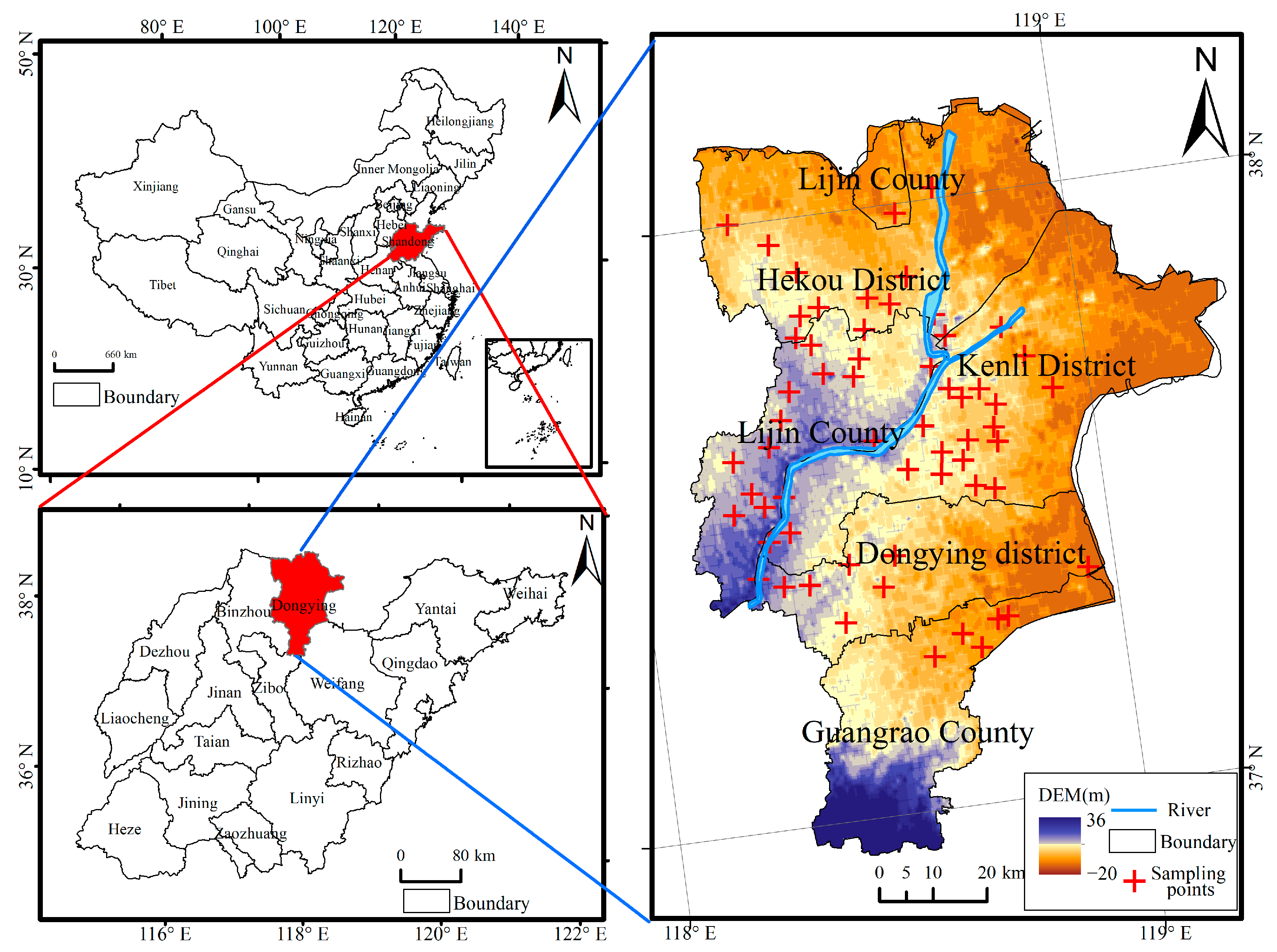
2.1. Study Area Overview

As shown in Figure 1, Dongying City is located in the northern part of Shandong Province (36°55′–38°10′N, 118°07′–119°10′E), known as the oil city and the Yellow River water city. Its coastline stretches from the Shunjiang Gou River mouth in the north to the Zimaigou River mouth in the south, with a total length of 412 km, and is situated at the mouth of the Yellow River. The city faces the sea to the east and north and is bordered by Binzhou City, Zibo City, and Weifang City to the west and south. The area has a temperate continental monsoon climate, with an elevation ranging from −20 to 36 m. The terrain slopes from the southwest to the northeast along the Yellow River. The annual average temperature is 12.5 °C, and the average annual precipitation is 550–600 mm, which makes it prone to both drought and waterlogging disasters. The major soil types include brown soil and sandy black soil. Due to the small pore sizes and compact nature of the soil, salts are difficult to leach, and the area experiences significant salinization due to the high salt content carried by rivers.

2.2. Data Collection and Preprocessing

2.2.1. Data Collection

Sample collection was conducted in October 2022 during the salt accumulation period, with a total of 87 measurement units (30 m × 30 m) being set up. For each sampling unit, GPS locations were recorded (Figure 1). Soil sample collection points were arranged in a five-point “plum–blossom” pattern, collecting soil samples from a 0–20 cm depth. Each sample from a unit was split into two portions: one for soil salinity determination and the other for moisture content measurement.

After collection, one portion of the soil samples was naturally air-dried, crushed, and sieved through a 1 mm mesh. It was then mixed evenly, and a 200 g sample was extracted using the quartering method. A 1:5 soil-to-water ratio extract was prepared for salinity analysis. The average salinity value of each sampling unit was then calculated. The other portion of the soil sample was oven-dried to determine moisture content. The processing of soil samples and the determination of both salinity and moisture content were carried out at the Analytical Testing Center of Shandong University of Technology.

Spectral data collection was synchronized with soil sample collection, conducted between 11:00 and 14:00 on clear, windless, or slightly windy days. A spectral radiometer (SVC HR1024i, Spectra Vista Corporation, Poughkeepsie, NY, USA) with a spectral range of 350 nm to 2500 nm and 1024 channels was used. Prior to spectral measurements, the spectrometer was calibrated with a white board. Depending on the sample, two observation methods were used at a 0.5 m sampling distance: (1) The field of view (FOV—the maximum angular extent of the observable spatial area captured by an optical instrument) was 25°; we used a vertical height of approximately 1.1 m, and ground diameter was around 0.5 m. Measurements were performed in 4 directions (with 90° rotations), with a 1 s sampling interval. Each direction was sampled 5 times, for a total of 20 measurements, and the average spectral reflectance was calculated. (2) The field of view (FOV) was 4°; the probe was positioned vertically to the sample, at a distance of 15 cm, with a ground diameter of approximately 5 cm. This method was applied similarly to the above-mentioned method.

2.2.2. Data Preprocessing

The exported spectral data were imported into Matlab R2022a (MathWorks, Inc., Natick, MA, USA) [42]. Due to the potential for noise interference during data collection, S-G (Savitzky-Golay-) filtering was applied to smooth and denoise the raw spectral data. S-G filtering was first proposed by Savitzky et al. in 1964 [43].

S-G filtering is a smoothing technique based on the local least squares method, used to eliminate noise in spectral sequence data. The core idea of S-G filtering is to fit a polynomial within the local neighborhood of each data point and then replace the original data point with the value derived from this fitted polynomial. This method preserves the higher-order derivative information of the data while removing noise, making it suitable for scenarios requiring the preservation of data sharpness [44].

For a spectral sequence $Y(t)$, where $t$ = 1, …, $N$ ($N$ is a positive integer), its adjacent $2k+1$ data points ($k$ is a positive integer) are considered. Within this local neighborhood, the $l$-th order polynomial can be fitted as follows:

$$o(t)=a_0+a_{1}t+a_2{t}^2+\cdots +a_l{t}^l$$

(1)

In the above equation, $o(t)$ denotes the fitted polynomial, and $a_j$ ($j$ = 0, 1, …, $l$) represents the polynomial coefficients; the objective is to determine the coefficients $a_j$ ($j$ = 0, 1, …, $l$) that minimize the squared error between the fitted polynomial and the original data within a local neighborhood.

$$E={\displaystyle \sum _{j=-k}^k{\left[Y\left(t+j\right)-o\left(t+j\right)\right]}^2}$$

(2)

In the above equation, $E$ denotes the squared error between the fitted polynomial and the original data; $k$ is a positive integer that determines the window length. The optimization problem is solved via the least squares method, yielding a system of linear equations for calculating the polynomial coefficients. Upon solving this linear system, the original data point $Y(t)$ is replaced by the fitted polynomial $o(t)$. Repeating this procedure for all data points ultimately generates the smoothed spectral sequence data.

To mitigate or eliminate baseline drift caused by scattering effects, the denoised data underwent Multiplicative Scatter Correction (MSC). MSC was first proposed by Geladi et al. [45].

MSC is a widely employed spectral preprocessing technique; after scatter correction, the resultant spectral data amplify absorption signatures related to constituent concentrations.

The specific MSC calculation procedure comprises the following:

(1)

The first step entails computing the average spectrum of spectra awaiting correction:

$$\overline{A}={\displaystyle \frac{{\displaystyle \sum _{i=1}^n{A}_i}}{n}}$$

(3)

(2)

The second step involves implementing univariate linear regressions against the reference spectrum to determine regression coefficients and biases for each sample:

$$A_i=m_i\overline{A}+b_i$$

(4)

(3)

Then, we correct the raw spectra:

$$A_{i(\mathrm{msc})}={\displaystyle \frac{A_i-b_i}{m_i}}$$

(5)

In the above equations, $A_i$ is the calibrated spectral data matrix; $\overline{A}$ denotes the mean spectrum vector obtained by averaging the near-infrared spectra at each wavelength after S-G smoothing; $a_i$ and $b_i$ represent the relative scaling coefficient and translational offset, respectively, derived from univariate linear regression against the mean spectrum.

Additionally, water vapor absorption bands, which could interfere with spectral measurements, were removed to reduce their impact on subsequent analyses. All preprocessing steps were conducted in Matlab R2022a [46].

To ensure that the training and validation samples had similar and evenly distributed values, the samples were sorted by their salinity levels. A gradient-based method was applied to divide the samples into two groups: a training set of 60 samples and a validation set of 27 samples. The distribution of samples between the two groups was nearly identical.

2.3. Research Methods

2.3.1. Fractional-Order Differentiation

FOD is an extension of integer-order differentiation, offering advantages such as “globality” and “memory.” Compared to integer-order differentiation, FOD is better able to highlight subtle and global changes in spectral data, improving the signal-to-noise ratio and reducing the impact of noise on the spectral data. This makes it a commonly used method in spectral data transformation [47]. Currently, the Grünwald–Letnikov (G–L) FOD method is popular due to its computational efficiency. For a continuous function f(x) defined on the interval [s, t], if the function has a continuous α-order derivative, the α-th derivative of f(x) at point t is given by Equation (1) [48]:

$${\mathrm{d}}_{\mathrm{t}}^{\alpha }f(x)=\underset{h\to 0}{\lim }{\displaystyle \frac{1}{h^{\alpha }}}{\displaystyle \sum _{m=0}^{[\frac{t-s}{h}]}{(-1)}^m}{\displaystyle \frac{\Gamma (\alpha +1)}{m!\Gamma (\alpha -m+1)}}f(\lambda -mh)$$

(6)

Here, λ is the hyperspectral wavelength in nm, f(λ) is the spectral reflectance, and h is the step size. The variables t and s represent the upper and lower limits of the differentiation, and Γ is the Gamma function. The value α represents the fractional order, where α = 0, 1, and 2 correspond to the original spectral data, first-order differentiation, and second-order differentiation, respectively.

In this study, the step size h was set to 1, with the wavelength ranges s and t representing the starting and ending wavelengths, respectively, and t − s = k. The α-order derivative of the hyperspectral data is as follows:

$$\begin{array}{c}{\displaystyle \frac{d^{\alpha }f(\lambda )}{d{\lambda }^{\alpha }}}\approx f\left(\lambda \right)+\left(-\alpha \right)f\left(\lambda -1\right)+{\displaystyle \frac{\left(-\alpha \right)\left(-\alpha +1\right)}{2}}f\left(\lambda -2\right)+\cdots \\ +{\displaystyle \frac{\Gamma \left(-\alpha +1\right)}{k!\left(-\alpha +k+1\right)}}f\left(\lambda -k\right)\end{array}$$

(7)

From Equation (2), it can be observed that the fractional-order derivative at point λ is influenced by all the values up to λ − 1, which demonstrates the “global” and “memory” characteristics of fractional-order derivatives. In this study, a step size of 0.2 was used to calculate the fractional-order derivatives of hyperspectral reflectance in the range from 0 to 2 orders. The entire process was implemented using Matlab R2022a [49].

2.3.2. Index Construction

Two-dimensional spectral indices are a commonly used method for the inversion of hyperspectral soil salinity data. Compared to one-dimensional spectral data, two-dimensional spectral indices can effectively account for the interrelationships between spectral bands. Based on the preprocessing and FOD of spectral data, 9 spectral indices were constructed. The optimal order and spectral band combinations for each index were identified based on their correlation coefficients with soil salinity. The calculation methods for the 9 spectral indices are shown in

Table 1. Spectral index calculation methods.

Spectral Index	Calculation Formula	Spectral Index	Calculation Formula
Normalized Difference Index (NDI) [20]	${\displaystyle \frac{R_i^{\alpha }-R_j^{\alpha }}{R_i^{\alpha }+R_j^{\alpha }}}$	Difference Index (DI) [20]	$R_i^{\alpha }-R_j^{\alpha }$
Optimal Spectral Index (OSI) [50]	${\displaystyle \frac{(1+0.45)\times (2R_j^{\alpha }+1)}{R_i^{\alpha }+0.45}}$	Ratio Index (RI) [20]	${\displaystyle \frac{R_i^{\alpha }}{R_j^{\alpha }}}$
Soil-Adjusted Spectral Index (SASI) [50]	${\displaystyle \frac{(1+0.5)\times (R_i^{\alpha }-R_j^{\alpha })}{R_i^{\alpha }+R_j^{\alpha }+0.5}}$	Product Index (PI) [50]	$R_i^{\alpha }\times R_j^{\alpha }$
Generalized Difference Index (GDI) [50]	${\displaystyle \frac{{R_i^{\alpha }}^2-{R_j^{\alpha }}^2}{{R_i^{\alpha }}^2+{R_j^{\alpha }}^2}}$	Sum Index (SI) [50]	$R_i^{\alpha }+R_j^{\alpha }$
		Nitrogen Plane Domain Index (NPDI) [50]	$(R_i^{\alpha }+R_j^{\alpha })\times R_j^{\alpha }$

[50].

In these equations, R_i and R_j represent reflectance values from different wavelengths, and α represents the fractional order.

2.3.3. Model Construction and Accuracy Evaluation

First proposed by Wold et al. in 1983, Partial Least Squares Regression is a multivariate statistical analysis method combining multiple linear regression with principal component analysis [51]. It is particularly useful when multicollinearity exists among independent variables and when the number of samples is fewer than the number of variables. Compared to traditional regression methods, PLSR performs better in regression modeling when these conditions are present [52].

Random Forest was first proposed by Breiman et al. in 2001 [53] and is an ensemble learning method based on classification and regression trees. It is capable of handling both classification and regression problems, performing dimensionality reduction, and demonstrating high speed and simplicity in training, with strong resistance to overfitting [54]. In this study, K-fold cross-validation (K = 10, selected due to the small-to-moderate dataset size) was applied to the training set alongside grid search optimization to enhance the generalization capability of the RF model [55]. The hyperparameter search spaces were configured as follows: number of decision trees (30, 50, 100, 150, 200, 250, 500), minimum leaf size (3, 5, 10, 15), and number of iterations (100, 200, 500, 1000, 1500, 2000, 2500). The optimal RF configuration comprised 100 decision trees, a minimum leaf size of 3 samples, and 2000 estimator iterations.

The development of CNN dates back to Hubel et al. in 1962 [56]. CNN models are deep learning models designed for feature extraction, classification, and regression. Compared to traditional machine learning algorithms, CNNs offer better generalization capabilities. The architecture consists of five main parts: the input layer, convolutional layer, activation layer, pooling layer, and fully connected layer [20]. In this study, we designed an 8-layer Convolutional Neural Network model. The model employed the Adam optimization algorithm, with hyperparameter tuning conducted using the same approach applied to the RF model. The final configurations comprised a maximum of 1200 training epochs, an initial learning rate of 0.01, and ReLU activation. To mitigate overfitting, a dropout layer was integrated, stochastically deactivating 10% of neural units during training.

All models were built and implemented using Matlab R2022a [57].

In this study, the model’s accuracy was evaluated using three metrics: the coefficient of determination R² [58], Root Mean Square Error (RMSE) [59], and Relative Percentage Deviation (RPD). A larger R² value and smaller RMSE indicate higher model accuracy, while a larger RPD indicates better predictive performance. RPD values were interpreted as follows: When RPD is >2, the model is considered to have excellent predictive ability. When RPD is between 1.8 and 2.0, the model has good predictive performance. When RPD is between 1.4 and 1.8, the model has moderate predictive ability. When RPD is between 1.0 and 1.4, the model has poor predictive performance, and when RPD is <1.0, the model’s predictive ability is very poor [60].

The formulas for R², RMSE, and RPD are as follows:

$$R^2=1-{\displaystyle \frac{{\displaystyle \sum _{i=1}^n{(y_i-{\widehat{y}}_i)}^2}}{{\displaystyle \sum _{i=1}^n{(y_i-\overline{y_i})}^2}}}$$

(8)

$$\mathrm{RMSE}=\sqrt{{\displaystyle \frac{1}{n}}{\displaystyle \sum _{i=1}^n{(y_i-{\widehat{y}}_i)}^2}}$$

(9)

$$\mathrm{SD}=\sqrt{{\displaystyle \frac{{\displaystyle \sum _{i=1}^n{(y_i-{\overline{y}}_i)}^2}}{n}}}$$

(10)

$$\mathrm{RPD}={\displaystyle \frac{\mathrm{SD}}{\mathrm{RMSE}}}$$

(11)

In the above equations, $y_i$ denotes the measured salt content of the sample, ${\widehat{y}}_i$ represents the predicted salt content, $n$ indicates the total number of samples, and $i$ corresponds to the sample identifier.

3. Results

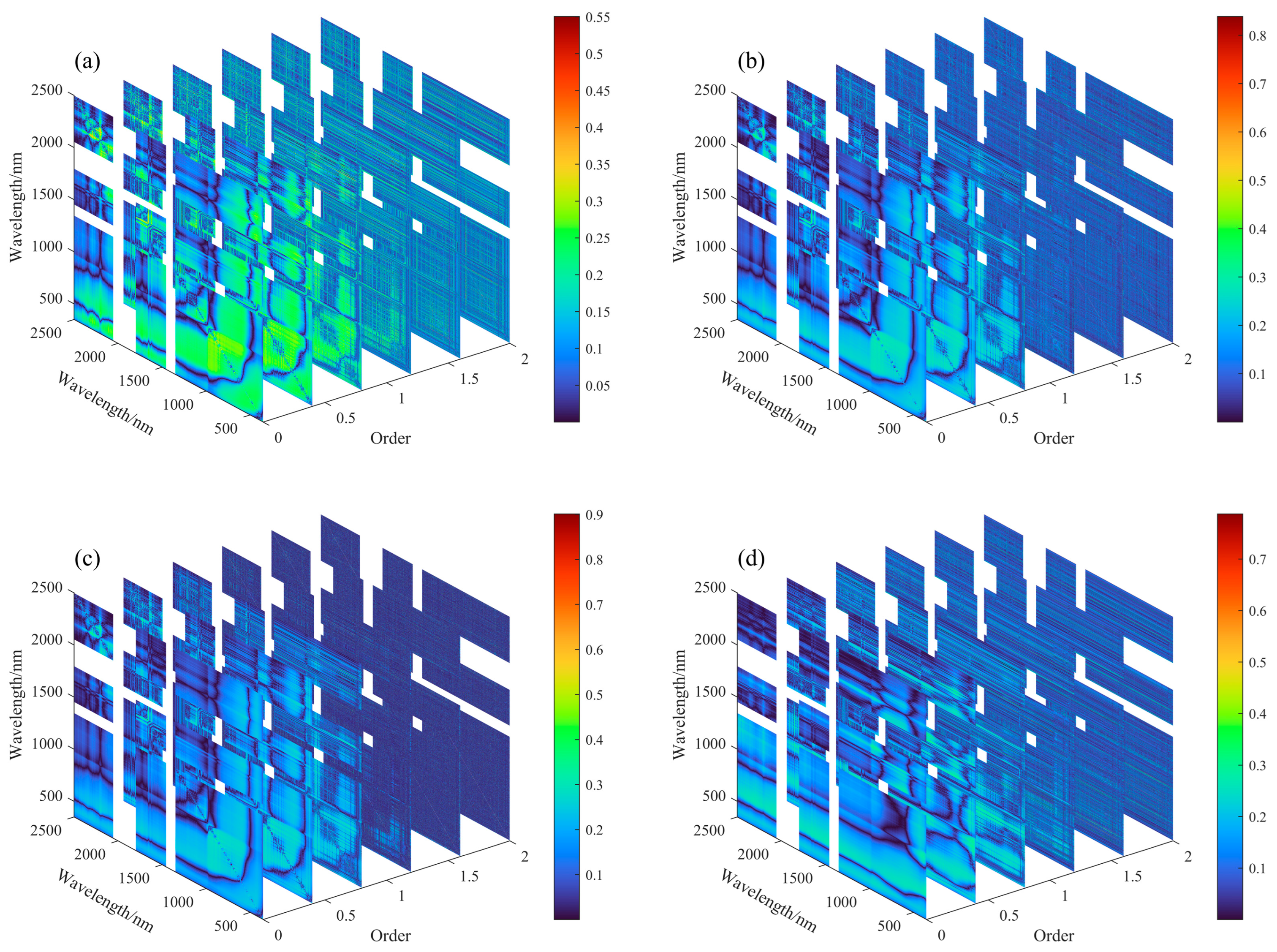
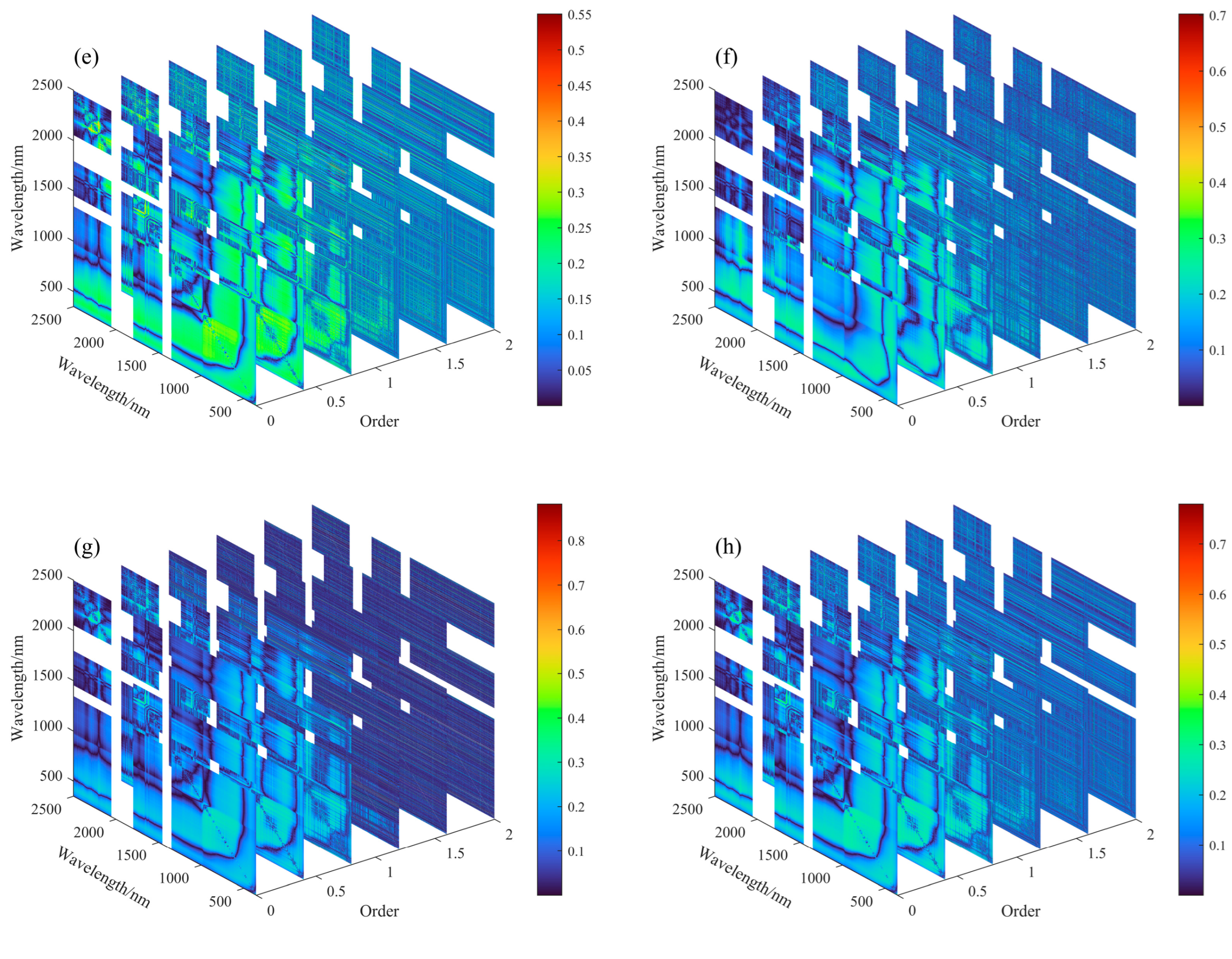
3.1. Spectral Curve Characteristics

The raw spectral curves of the samples are presented in Figure 2a. The general characteristics of the curves are similar, with spectral reflectance ranging from 5% to 45%. As the wavelength increases, the spectral reflectance increases rapidly between 350 and 1000 nm, before increasing more slowly between 1000 and 2000 nm and then showing a decreasing trend. The rapid increase in soil spectral reflectance within the 350–1000 nm band is primarily driven by salt-induced surface scattering enhancement (e.g., salt crust formation) and diminished absorption by iron oxides/organic matter [61]. The gradual ascending trend in the 1000–2000 nm range stems from dual suppression mechanisms: salt crystallization obscuring vibrational absorption of clay minerals (e.g., Al-OH) and competing water absorption [33]. Beyond 2000 nm, reflectance decline is attributed to intensified vibrational absorption in salt minerals (e.g., gypsum at 2200 nm) and deep-layer clay lattice vibrations, where attenuation amplitude exhibits significant negative correlation with salt enrichment [62]. This collectively demonstrates how salinization systematically regulates spectral responses through alterations in soil physical structure (crust porosity), chemical composition (salt crystallization), and moisture status, shaping comprehensive response patterns. Notable water vapor absorption bands occur at wavelengths between 1350 and 1450 nm [63] as well as 1800 and 2050 nm [64]. To eliminate or reduce the impact of water vapor absorption bands [20], spectral noise, and baseline drift on spectral reflectance, preprocessing steps including removal of water vapor absorption bands, S-G filtering, and MSC were applied. As shown in Figure 2b, the spectral curve after preprocessing exhibits a smoother and more concentrated trend without significant changes in its shape.

As shown in Figure 3, the preprocessed spectra were subjected to fractional-order differential transformations at intervals of 0.2 orders, resulting in a total of 11 differential transformations from the 0th order to the 2nd order. The 0th order corresponds to the raw spectral curve, which shows the most fluctuation. As the differential order increases, the spectral curve becomes progressively smoother. The 0–0.6th-order range maintains the general shape of the original curve, while in the 0.8–2nd-order range, the curve shows minimal change and approaches a straight line at y = 0, with baseline drift being gradually eliminated. At lower orders, as the order increases, the peak and valley features become more prominent. Compared with the zeroth order, the first- and second-order differentials show more significant changes in the curve features, while the FOD reflects the spectral curve changes more effectively.

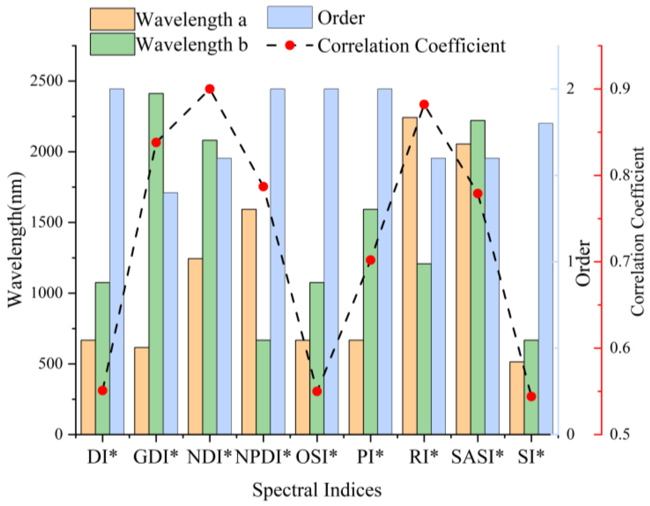
3.2. Feature Extraction

Nine spectral indices were calculated between different wavelengths for the FOD spectra, and the absolute values of the correlation coefficients between the spectral indices and soil salinity at various differential orders were computed.

Using the SI as an example, a correlation coefficient matrix was plotted, as shown in Figure 4i. The horizontal and vertical axes represent the spectral wavelengths of the soil samples, with color gradients from blue to red indicating increasing absolute correlation coefficients. As seen in Figure 4, the highest absolute correlation coefficient in the original spectrum is 0.349. After applying FOD transformations, the maximum absolute correlation coefficient for each differential order exceeds 0.349, suggesting that FOD significantly improves the correlation between spectral information and salinity. As the order increases, the maximum correlation coefficient generally increases, peaking at the 1.8th order with a value of 0.544. High-correlation wavelength combinations occur in the spectral ranges of 350–400 nm and 700–1000 nm, 500–700 nm and 1500–1600 nm, as well as 1000–1300 nm and 2100–2200 nm. The spectral band of 350–400 nm demonstrates sensitivity to soil organic matter, iron oxides, and surface coloration, wherein elevated salinity disrupts soil aggregates and induces crust development, augmenting surface roughness to diminish reflectance in the shortwave spectrum [65]; the 700–1000 nm region primarily responds to alterations in soil texture and structure, as salinity-induced particle rearrangement modifies light-scattering efficiency, generating distinctive reflectance signatures [66]; the 500–700 nm range detects chromatic variations in soils, with high salinity causing visible discoloration (e.g., white salt efflorescence) that substantially elevates reflectance [67]; the 1500–1600 nm band falls within the absorption domain of water molecules (H₂O) and hydroxyl groups (–OH), where salinity alters reflectance by affecting water retention capacity and moisture distribution [68]; the 1000–1300 nm region exhibits sensitivity to aluminum hydroxyl (Al–OH) absorption features in clay minerals such as montmorillonite and kaolinite [69]; and the 2100–2200 nm band corresponds to the primary vibrational absorption maxima of sulfates (e.g., gypsum) and carbonates [68]. As the order increases, the blue areas expand, indicating that the number of low-correlation combinations increases, and the optimal spectral combinations become more apparent.

Based on the maximum absolute correlation coefficients of different spectral indices with salinity, the corresponding wavelength combinations and differential orders were selected to determine the optimal wavelength and order combinations for each spectral index, as shown in Figure 5.

From Figure 5, it can be seen that 667 nm appears most frequently among the spectral indices, followed by 1075 nm. The optimal orders for different spectral indices are primarily the 2nd order and fractional orders, suggesting that after differential transformation, the spectral indices significantly improve the correlation between spectral information and soil salinity compared to the original 0^th-order spectrum. The maximum absolute correlation coefficient is 0.90 for NDI, followed by 0.882 for RI, and the lowest is 0.550 for OSI. Among the different optimal spectral indices, the 2nd order appears most frequently, followed by the 1.6th order.

Based on Figure 5, the optimal wavelength and order combinations for each spectral index were determined, and 9 spectral indices were calculated for 87 samples to construct sensitive features for subsequent modeling and regression analysis.

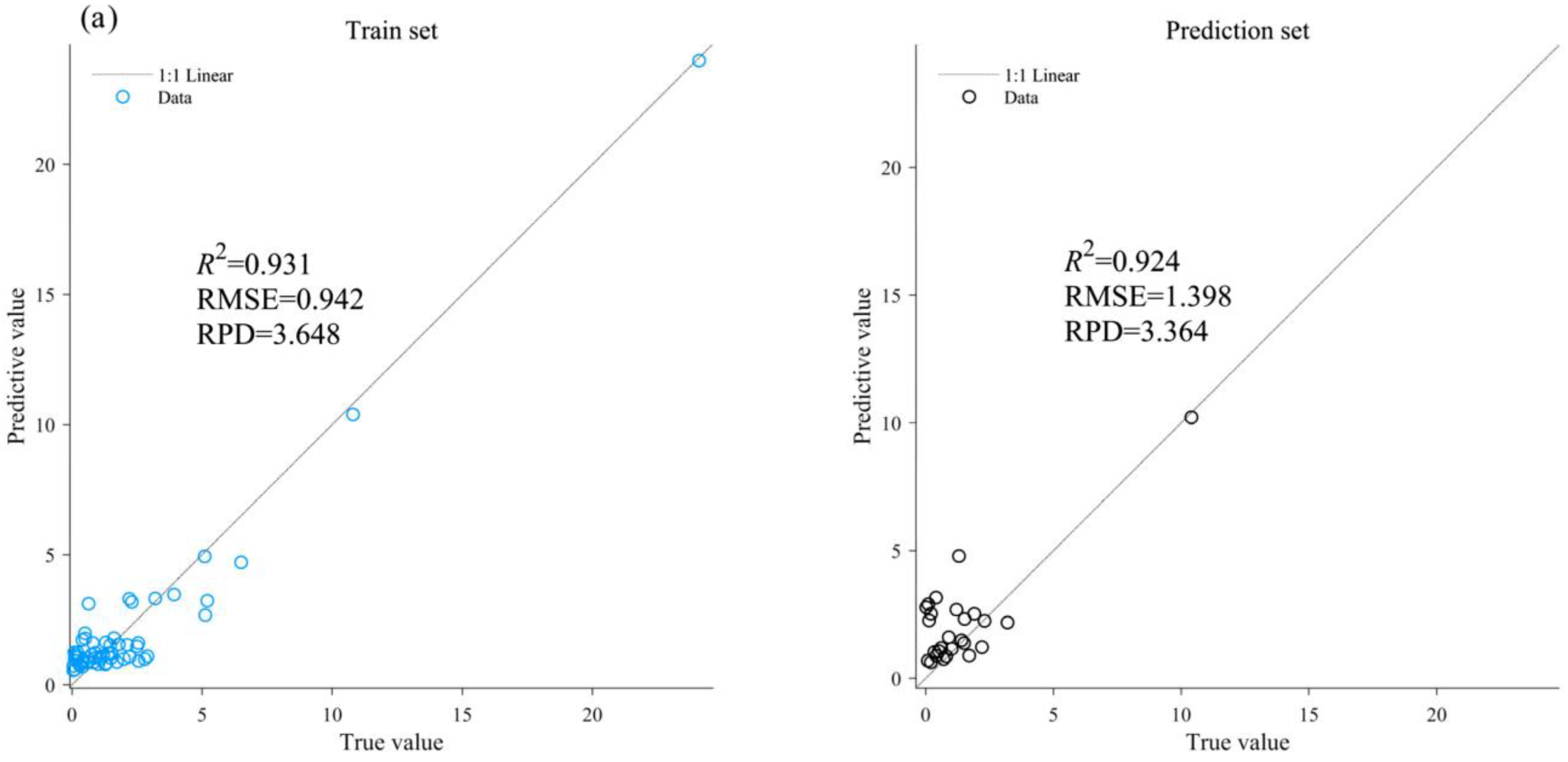
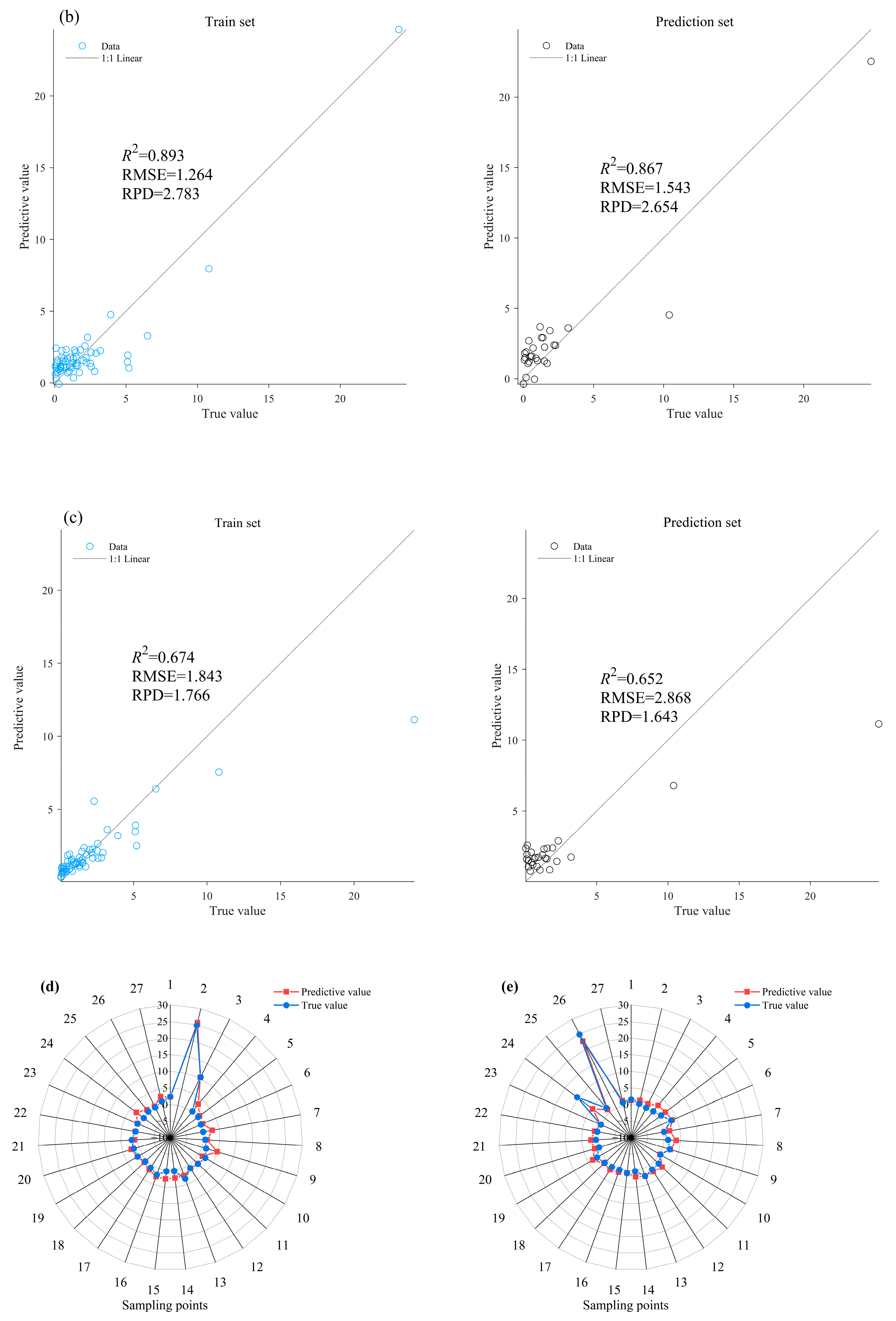
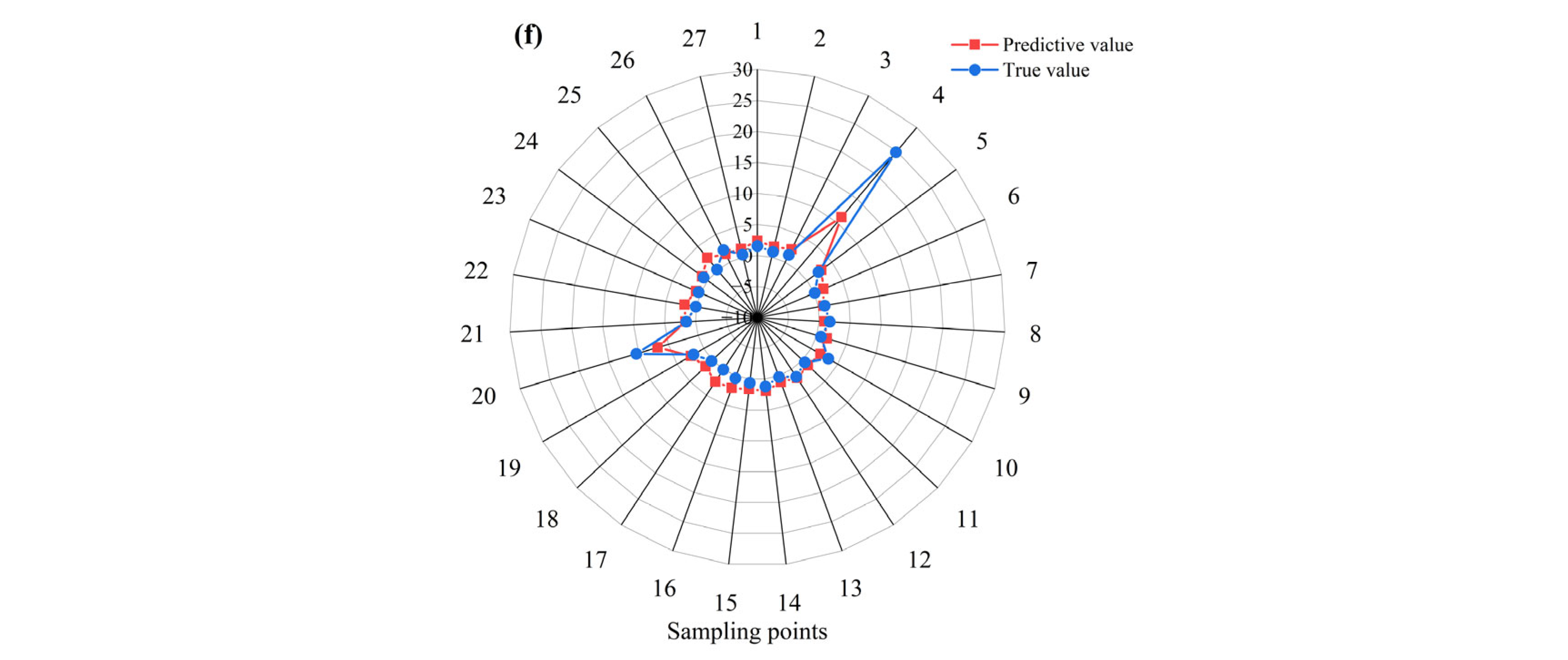
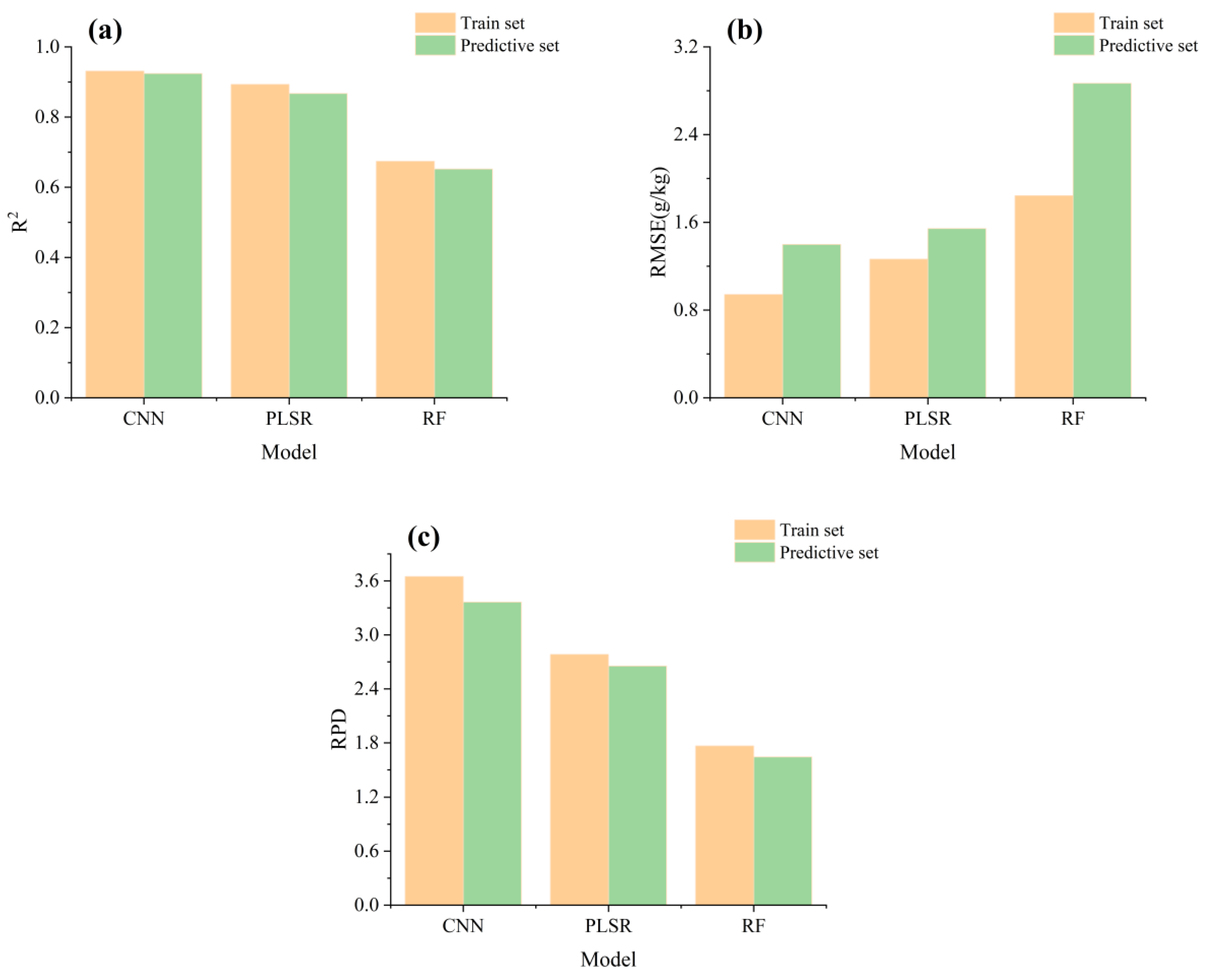
3.3. Model Result Analysis

Based on the optimal wavelength combinations and differential orders for the different spectral indices, along with the corresponding soil salinity values for the sample points, the RF, PLSR, and CNN models were trained using all of the training set (the hyperparameters of the model were determined via 10-fold cross-validation and grid search techniques applied to the training set), and the results were validated with the validation set. The accuracy evaluation results are shown in Figure 6 and Figure 7 as well as

Table 2. Accuracy evaluation of different models.

Model	Train Set			Predictive Set
	R2	RPD	RMSE (g/kg)	R2	RPD	RMSE (g/kg)
CNN	0.931	3.648	0.942	0.924	3.364	1.398
PLSR	0.893	2.783	1.264	0.867	2.654	1.543
RF	0.674	1.766	1.843	0.652	1.643	2.868

.

From Figure 6 and Figure 7 as well as Table 2, it can be observed that the CNN model achieves the highest R² for both the training and prediction sets, reaching 0.9. The PLSR model follows with an R² of 0.85, while the RF model performs the worst, with an R² not exceeding 0.7. The R² values for the training set are 0.931 for CNN, 0.893 for PLSR, and 0.674 for RF. The corresponding values for the prediction set are 0.924, 0.867, and 0.652, respectively. Compared to PLSR and RF, the CNN model shows improvements of 0.038 and 0.257 in R² for the training set and improvements of 0.057 and 0.272 for the prediction set. In the CNN model, the RPD for both the training and prediction sets is greater than 3, indicating excellent predictive capability. In the PLSR model, the RPD for both sets is greater than 2, suggesting very good predictive performance, though it is slightly inferior to CNN. In the RF model, the RPD ranges from 1.4 to 1.8, indicating average predictive ability. The CNN model has the smallest RMSE for both the training and prediction sets, with values of 0.942 g/kg and 1.398 g/kg, respectively. Compared to PLSR and RF, the CNN model reduces the RMSE for the training set by 0.322 g/kg and 0.901 g/kg, and for the prediction set, the RMSE is reduced by 0.145 g/kg and 1.470 g/kg, respectively.

These analyses suggest that, compared to the PLSR and RF models, the CNN model based on FOD demonstrates superior accuracy and predictive capability, followed by PLSR, while the RF model exhibits the lowest predictive accuracy and capability.

4. Discussion

4.1. Merits of Fractional Calculus

Hyperspectral data has the advantage of containing rich and continuous information commonly used for monitoring soil, crops, and other properties [70]. However, due to the large data volume, redundancy between wavelengths, and strong collinearity, hyperspectral data models often suffer from poor adaptability [71]. FOD, combined with spectral indices, effectively extracts the gradual information of data transformations and utilizes the rich information from hyperspectral data, reducing data redundancy and improving model applicability. The hyperspectral estimation model for soil salinity based on FOD showed superior stability in Zhao et al. (2021), but characteristic band discrepancies (581–774 nm vs. 1000–1500 nm herein) arise from divergent soil mineral composition, vegetation coverage, and moisture content between Bosten Lake oasis and Dongying City [72]. In the 581–774 nm visible-near-infrared range, the Bosten Lake exhibits higher reflectance due to highly reflective salt crusts formed on salinized topsoil, sparse vegetation, and arid conditions [73], whereas Dongying City shows lower reflectance resulting from strong organic matter absorption, dense crop cover (with pronounced red-edge effects), and higher soil moisture. In the 1000–1500 nm shortwave infrared region, the Bosten Lake’s elevated reflectance is attributed to low moisture levels and salt-induced suppression of water absorption, while Dongying City’s reduced reflectance stems from intense water absorption in humid soils (e.g., absorption trough near 1450 nm) and hydroxyl absorption features of clay minerals (e.g., montmorillonite) [74]. Regarding inversion model accuracy, Zhao et al. achieved R² = 0.83 using PLSR, whereas this study attained superior performance (R² = 0.931) due to (1) its incorporation of spectral indices as feature variables to capture inter-band synergies and (2) the CNN model’s capacity to resolve complex nonlinear relationships between bands, contrasting with PLSR’s limitations in handling strongly collinear data [72]. Notably, both the above study and the current research confirm that fractional-order differential transformation, compared to raw spectral data, can enhance model adaptability and provide better stability in data prediction. Concretely, -FOD captures gradual spectral variations unresolved by integer-order differentiation through continuous order adjustments (e.g., 0.2-order steps) [75]. By exploring multiple orders, it identifies optimal transformation orders and band combinations exhibiting peak correlations with target parameters [76]. Through the nonlinear feature enhancement of spectral information, it amplifies subtle spectral differences and elevates the signal-to-noise ratios of sensitive bands [77]. Integrating FOD with spectral indices extends the mathematical–physical framework of spectral analysis from Euclidean to fractional-dimensional spaces, enhancing model capability in resolving complex spectral characteristics to better capture intricate synergistic relationships among spectral features, where FOD amplifies such synergies, thereby strengthening model adaptability and stability [78].

4.2. Advantages and Adaptability of Spectral Indices

Spectral indices enhance the inversion accuracy of models by comprehensively integrating the response characteristics of multiple spectral reflectance bands to soil salinity, thereby improving the coupling relationships between spectral datasets. Chen (2023) found a 1.1-order SVM model optimal for Yinchuan Plain’s soil salinization (R² = 0.839, RMSE = 0.96), while our study demonstrates superior performance (R² = 0.924, RMSE = 1.398 g/kg, RPD = 3.364), particularly in RMSE enhancement [79]. Significant variations exist in sensitive band selection between this study (667 nm, 1075 nm, 1244 nm, 2081 nm) and Chen’s research (401 nm, 740 nm, 2098 nm, 2099 nm). The Ningxia Plain, situated in an arid climate zone with sulfate chloride-mixed soil types, exhibits salt enrichment at the surface due to intense evaporation and irrigated agriculture, rendering visible blue bands (401 nm) and shortwave infrared (2099 nm) sensitive to sulfate crystallization and salt crust characteristics. Conversely, Dongying City, as a coastal saline area dominated by sodium chloride soils, experiences significant tidal and groundwater influences where coupled interactions of salt migration with clay minerals and halophytic vegetation enhance responses to chloride ions and soil moisture in red bands (667 nm) as well as in the mid-infrared (2081 nm) range [80]. In this study, nine spectral indices were constructed, and the highest correlation coefficient with soil salinity was found for the NDI and RI indices. Huang Huayu et al. found the strongest correlation between surface soil salinity and the difference index (DI) during hyperspectral inversion in the Yinbei region of Ningxia, with characteristic bands at 2240 nm and 1640 nm [50], differing from the bands identified in this study. The Yinbei area, characterized by an arid climate and sulfate chloride-mixed salts, features sandy soils with significant spatial heterogeneity of salt crusts. DI effectively enhances contrast in salt-affected areas through subtraction operations applied to shortwave infrared bands (sulfate absorption at 1640 nm; chloride reflection at 2240 nm). Conversely, Dongying City represents a coastal saline region dominated by sodium chloride, where heavy-textured soils and tidal moisture fluctuations lead the normalized index (NDI) to suppress soil humidity and clay mineral interference via ratio processing of mid-infrared bands (weak clay absorption at 1244 nm; strong chloride ion absorption at 2081 nm), thereby precisely extracting homogeneous salt signals. These disparities demonstrate that spectral indices require adaptation to regional salt types, soil textures, and environmental noise sources: arid regions prioritize salt crust heterogeneity enhancement, whereas coastal areas necessitate balancing spectral coupling effects among salinity, moisture, and minerals.

4.3. Superiority of Convolutional Neural Network (CNN) Models

Deep learning models like CNNs offer powerful advantages in data dimensionality reduction and feature extraction, making them suitable for processing large datasets with excellent model performance. The convolutional layers of CNNs efficiently extract local features while preserving spatial configuration through localized receptive fields and weight-sharing mechanisms, substantially reducing parameter volume; the pooling layers (e.g., max pooling, average pooling) achieve spatial dimensionality reduction via downsampling, filtering redundant information while enhancing feature translation invariance to improve model robustness. Furthermore, multi-layer cascaded architectures with alternating convolution-pooling stacking enable progressive abstraction from low-level to high-level features, with optimized techniques such as Depthwise Separable Convolutions (DSCs) further reducing computational complexity [81]. In this study, the CNN model outperformed the PLSR and RF models in terms of both training and prediction accuracy. Zhao et al. (2024) used CNNs to estimate soil salinity in the Jiaozuo Ma village mining area, and the optimal CNN model outperformed BP neural networks (BPNNs) and RF, improving RPD by 7.53 and 1.25, respectively [82]. Both studies align with the findings in this research, further demonstrating the strength of CNN models in regression-based predictions.

5. Conclusions

This study took Dongying City as its research object and considered hyperspectral data and soil salinity measurements. The preprocessed spectral data underwent fractional-order differential transformation, upon which nine types of two-dimensional spectral indices were constructed. By calculating the correlation coefficients between spectral indices with varying fractional orders and wavelength combinations and soil salinity, the optimal wavelength combinations and corresponding transformations for each spectral index were selected. Subsequently, CNN, PLSR, and RF models were constructed to invert soil salinity. Key conclusions that can be drawn from our results include the following:

(1)

Compared to integer-order differentiation, FOD effectively highlights gradual changes in spectral curve variations.

(2)

FOD significantly improves the correlation between spectral indices and soil salinity compared to the original spectrum.

(3)

The optimal NDI (1244 nm, 2081 nm) and RI (2242 nm, 1208 nm) spectral indices at the 1.6th order show the highest correlation with soil salinity, with correlation coefficients of 0.90 and 0.882, respectively.

(4)

The CNN model achieved the highest inversion accuracy, improving the RPD of the prediction set by 0.710 and 1.721, improving R² by 0.057 and 0.272, and reducing RMSE by 0.145 g/kg and 1.470 g/kg compared to the PLSR and RF models.

References

1. Zhang, J.K.; Song, N.P.; Yang, S.Q.; Wang, X.; Chen, L.; Wang, Q.X. Spatial Variation Characteristics of Soil Salinity in Desert Steppe. Chin. J. Soil Sci. 2025, 56, 87–95. [Google Scholar]
2. Corwin, D.L. Climate change impacts on soil salinity in agricultural areas. Eur. J. Soil Sci. 2021, 72, 842–862. [Google Scholar]
3. Chen, K.; Li, C.; Tang, R. Estimation of nitrogen concentration in rubber trees using fractional calculus augmented NIR spectra. Ind. Crops Prod. 2017, 108, 831–839. [Google Scholar]
4. Gorji, T.; Yildirim, A.; Hamzehpour, N.; Sertel, E. Soil salinity analysis of Urmia Lake Basin using Landsat-8 OLl and Sentinel-2A based spectral indices and electrical conductivity measurements. Ecol. Indic. 2020, 112, 106173. [Google Scholar]
5. Allbed, A.; Kumar, L.; Sinha, P. Mapping and modelling spatial variation in soil salinity in the Al Hassa Oasis based on remote sensing indicators and regression techniques. Remote Sens. 2014, 6, 1137–1157. [Google Scholar]
6. Zhang, S.Y.; Yue, C.; Yuan, G.L.; Yuan, S.; Pang, W.Q.; Li, J. Salinization inversion model based on ENDVI-SI3 characteristic space and risk assessment. Remote Sens. Nat. Resour. 2022, 34, 136–143. [Google Scholar]
7. Wu, Y.H.; Zhao, H.Q.; Mao, J.H.; Jin, Q.; Wang, X.F.; Li, M.Y. Study on Hyperspectral Inversion Model of Soil Heavy Metals in TypicalLead-Linc Mining Areas. Spectrosc. Spectr. Anal. 2024, 44, 1740–1750. [Google Scholar]
8. He, S.; Zhang, S.; Tian, J.; Lu, X. UAV hyperspectral inversion of Suaeda Salsa leaf area index in coastal wetlands combined with multimodal data. Nat. Remote Sens. Bull. 2023, 27, 1441–1453. [Google Scholar]
9. Li, H.; Yu, H.; Cao, Y.Y.; Hao, Z.Y.; Yang, W.; Li, M.Z. Hyperspectral Prediction of Soil Organic Matter Content Using CARS-CNN Modelling. Spectrosc. Spect. Anal. 2024, 44, 2303–2309. [Google Scholar]
10. Li, J.; Chen, C.; Wang, Z. Inversion of High Spectral Characteristics of Soil Salt in Arid Area Based on Different Transform Forms. Res. Soil Water Conserv. 2018, 25, 197–201. [Google Scholar]
11. Li, Z.; Su, W.Z.; Li, X.G.; Wang, Y.F.; Mao, D.L.; Mamattursum, E. Modeling and Verification of Soil Salt Content Based on Hyperspectral Characteristic Parameter Optimization. Xinjiang Agric. Sci. 2021, 58, 2342–2352. [Google Scholar]
12. Wang, Y.J.; Gao, X.M.; Bao, S.M.; Li, W.; Fu, Y.; Wu, R.; Wang, J.Y.; Guo, L.Y. Prediction model of salt content in salinized soil based on hyperspectral data. Agric. Eng. 2024, 14, 113–120. [Google Scholar]
13. Huang, S.; Ding, J.L.; Li, X.; Yang, A.X. Research of Soil and Water Conservation. Chin. J. Soil Sci. 2016, 47, 1042–1048. [Google Scholar]
14. Zhang, X.J.; Zhang, Z.; Yang, X.M.; Song, L.L.; Wang, J.R.; Wang, F. Estimation of Salt and Water Content in Jingdian Irrigation Area Based on Hyperspectral of Salinized Soils. J. Gansu For. Sci. Technol. 2024, 49, 60–66. [Google Scholar]
15. Tian, A.H.; Zhao, J.S.; Zhang, S.J.; Fu, C.B.; Xiong, H.G. Hyperspectral estimation of saline soil electrical conductivity based on fractional derivative. Chin. J. Eco-Agric. 2020, 28, 599–607. [Google Scholar]
16. Leyden, K.; Goodwine, B. Fractional-order system identification for health monitoring. Nonlinear Dyn. 2018, 92, 1317–1334. [Google Scholar]
17. Zhang, W.W.; Yang, K.M.; Xia, T.; Liu, C.; Sun, T.T. Analysis of fractional-order derivatives and copper content in corn leaves. Sci. Technol. Eng. 2017, 17, 33–38. [Google Scholar]
18. Wang, J.; Ding, J.; Abulimiti, A.; Cai, L. Estimation of soil salinity using various modeling methods and VIS–NIR spectroscopy, Ebinur Lake Wetland, Northwest China. PeerJ. 2018, 6, e4703. [Google Scholar]
19. Fu, C.; Gan, S.; Yuan, X.; Xiong, H.; Tian, A. Impact of fractional calculus on correlation coefficients between available po-tassium and spectral data in hyperspectral and Landsat 8 imagery. Mathematics 2019, 7, 488. [Google Scholar]
20. Sun, Y.N.; Li, X.Y.; Shi, H.B.; Ma, H.Y.; Wang, W.G.; Cui, J.Q.; Chen, C. Optimizing the inversion of soil salt in salinized wasteland using hyperspectral data from remote sensing. Trans. Chin. Soc. Agric. Eng. 2022, 38, 101–111. [Google Scholar]
21. Zhang, B. Advancement of hyperspectral image processing and information extraction. J. Remote Sens. 2016, 20, 1062–1090. [Google Scholar]
22. Wang, S.; Chen, Y.; Wang, M.; Zhao, Y.; Li, J. SPA-Based Methods for the Quantitative Estimation of the Soil Salt Content in Saline-Alkali Land from Field Spectroscopy Data: A Case Study from the Yellow River Irrigation Regions. Remote Sens. 2019, 11, 967. [Google Scholar]
23. Wang, X.; Zhao, C.; Li, Z.; Huang, J. Modeling risk assessment of soil heavy metal pollution using partial least squares and fuzzy logic: A case study of a gully type coal-based solid waste dumpsite. Environ. Pollut. 2024, 352, 124147. [Google Scholar]
24. Guo, Y.K.; Zhang, S.A.; Wang, J.J.; Zhang, Q.; Xie, X.F. Feature variable selection combined with SVM for hyperspectral in-version of cultivated soil Hg content. Eng. Surv. Map. 2022, 31, 17–23. [Google Scholar]
25. Cheng, J.K.; Feng, X.X.; Chen, L.B.; Gao, T.Y.; Du, M.J.; Liu, Z.Y. Optimal inversion model for cultivated land soil sality hased on UAV hyperspectral data. Chin. J. Appl. Ecol. 2024, 35, 3085–3094. [Google Scholar]
26. Zhang, Z.P.; Ding, J.L.; Wang, J.Z.; Ge, X.Y.; Li, Z.S. Quantitative Estimation of Soil Organic Matter Content Using Three-Dimensional Spectral Index: A Case Study of the Ebinur Lake Basin in Xinjiang. Spectrosc. Spectral Anal. 2020, 40, 1514–1522. [Google Scholar]
27. Tang, Z.R.; Wu, T.; Tan, S.L.; Yue, S.R. Soil salinization monitoring model based on remote sensing derivative processing and optimal spectral index. Hubei Agric. Sci. 2024, 63, 223–230. [Google Scholar]
28. Hong, G.J.; Xie, J.F.; Zhang, L.; Fan, Z.Q.; Yu, C.L.; Fu, X.B.; Li, X. Monitoring soil salinization of cotton fields in the Aral Reclamation Area using multispectral imaging. Arid Zone Res. 2024, 41, 894–904. [Google Scholar]
29. Wang, W.Y.; Peng, J.B.; Zhu, W.X.; Yang, B.; Liu, Z.; Gong, H.R.; Wang, J.D.; Yang, T.; Lou, J.Y.; Sun, Z.G. Study on retrieval method of soil organic matter in salinity soil using unmanned aerial vehicle remote sensing. J. Geoinf. Sci. 2024, 26, 736–752. [Google Scholar]
30. Long, W.Y.; Shi, J.F.; Li, S.Y.; Sun, J.J.; Wang, Y.G. Evaluation of multimodel inversion effects on soil salinity in oasis basin. Arid Zone Res. 2024, 41, 1120–1130. [Google Scholar]
31. Zhang, Z.T.; Tai, X.; Yang, N.; Zhang, J.R.; Huang, X.Y.; Chen, Q.D. UAV Multispectral Remote Sensing Soil Salinity Inversion Based on Different Fractional Vegetation Coverages. Trans. Chin. Soc. Agric. Mach. 2022, 53, 220–230. [Google Scholar]
32. Bian, H.Q.; Wang, X.M. Estimation of soil salinity in cultivated layers of oasis in arid areas based on multispectral images. J. Arid Land Resour. Environ. 2022, 36, 110–118. [Google Scholar]
33. Zhao, X.Y.; Xi, H.Y.; Zhao, J.; Ma, K.H.; Cheng, W.J.; Chen, Y.Q. Inversion and spatial distribution characteristics of soil salinity in Alxa area, China. J. Des. Res. 2023, 43, 27–36. [Google Scholar]
34. Dong, X.X.; Han, X.; Yang, X.; He, Z.J.; Qiao, X.Y.; Zhu, H.L. A prediction model for dynamic alloy addition after converter based on CNN-LSSVM. Iron Steel. 2025, 60, 75–83. [Google Scholar]
35. Nie, X.J.; Hong, W.W.; Gill, A.; Yu, H.Y.; Chen, X.D. Hyperspectral estimation of coal-derived carbon mass fraction in mine soil based on the CWT-CARS-CNN integrated method. J. Henan Polytech. Univ. (Nat. Sci.) 2024, 43, 91–100. [Google Scholar]
36. Mashimbye, Z.E.; Cho, M.A.; Nell, J.P.; Clercq, W.P.D. Model-based integrated methods for quantitative estimation of soil salinity from hyperspectral remote sensing data: A case study of selected South African soils. Pedosphere 2012, 22, 640–649. [Google Scholar]
37. Kasim, N.; Maihemuti, B.; Sawut, R.; Abliz, A.; Dong, C.; Abdumutallip, M. Quantitative Estimation of Soil Salinization in an Arid Region of the Keriya Oasis Based on Multidimensional Modeling. Water 2020, 12, 880. [Google Scholar] [CrossRef]
38. Kahaer, Y.; Tashpolat, N.; Shi, Q.; Liu, S. Possibility of Zhuhai-1 hyperspectral imagery for monitoring salinized soil moisture content using fractional order differentially optimized spectral indices. Water 2020, 12, 3360. [Google Scholar] [CrossRef]
39. Farifteh, J.; Meer, F.V.; Atzberger, C.; Carranza, E.J.M. Quantitative analysis of salt-affected soil reflectance spectra: A comparison of two adaptive methods (PLSR and ANN). Remote Sens. Environ. 2007, 110, 59–78. [Google Scholar]
40. Das, A.; Bhattacharya, B.K.; Setia, R.; Jayasree, G.; Das, B.S. A novel method for detecting soil salinity using AVIRIS-NG imaging spectroscopy and ensemble machine learning. ISPRS J. Photogramm. Remote Sens. 2023, 200, 191–212. [Google Scholar]
41. Kazemi, G.M.; Blaschke, T.; Hossein, H.V.; Weng, Q.H.; Kamran, K.V.; Li, Z.L. A comparison between sentinel-2 and landsat 8 OLI satellite images for soil salinity distribution mapping using a deep learning convolutional neural network. Can. J. Remote Sens. 2022, 48, 452–468. [Google Scholar]
42. Li, J.Q.; Feng, Y.H.; Chen, S.H.; Wang, Z.A.; Liu, P.; Liang, Z.Y.; Sun, F.F.; Chen, R. Estimation of soil organic matter and total nitrogen based on hyperspectral technology. Xinjiang Agric. Sci. 2024, 61, 2491–2499. [Google Scholar]
43. Savitzky, A.; Golay, M.J.E. Smoothing and differentiation of data by simplified least squares procedures. Anal. Chem. 1964, 36, 1627–1639. [Google Scholar]
44. Yuan, C.; Zhang, H.; Ling, Y.H.; Sun, Y.; Huang, D.L.; Zhang, N.; Hu, F.J. Multiscale smoothing preprocessing method based on wavelet transform and S-G filtering. Forg. Stamp. Technol. 2023, 48, 140–155. [Google Scholar]
45. Geladi, P.; MacDougall, D.; Martens, H. Linearization and scatter-correction for near-infrared reflectance spectra of meat. Appl. Spectrosc. 1985, 39, 491–500. [Google Scholar]
46. Zhou, F.X.; Teng, X.S.; Hao, J.M.; Wang, L.Y. Applicability of Different Fractional Order Differential Forms in the Hyperspectral Inversion of Saline Soil Conductivity. Spectrosc. Spectr. Anal. 2025, 45, 272–281. [Google Scholar]
47. Hong, Y.S.; Shen, R.L.; Cheng, H.; Chen, Y.Y.; Zhang, Y.; Liu, Y.L.; Zhou, M.; Liu, Y.; Liu, Y.F. Estimating lead and zinc con-centrations in peri-urban agricultural soils using reflectance spectroscopy: Effects of fractional-order derivatives and random forest algorithms. Sci. Total. Environ. 2019, 651, 1969–1982. [Google Scholar]
48. Jing, X.; Zhang, T.; Zou, Q.; Yan, J.M.; Dong, Y.Y. Construction of remote sensing monitoring model of wheat stripe rust based on fractional-order differential spectral index. Trans. Chin. Soc. Agric. Eng. 2021, 37, 142–151. [Google Scholar]
49. Liu, J.L.; Wang, F.; Han, J.Q.; Ge, W.Y.; Liu, Y.H.; Lin, Y.Y. Study on spectral characteristics and quantitative estimation of soil salinity based on Fractional Order Derivative. Remote Sens. Technol. Appl. 2025, 40, 344–358. [Google Scholar]
50. Huang, H.Y.; Ding, Q.D.; Zhang, J.H.; Pan, X.; Zhou, Y.H.; Jia, K.L. Ground-hased hyperspectral inversion of salinization and alkalinization of different soil layers in farmland in Yinbei area, Ningxia, China. Chin. J. Appl. Ecol. 2024, 35, 3073–3084. [Google Scholar]
51. Wold, H. Systems Analysis by Partial Least Squares; IIASA Collaborative Paper; IIASA: Mödling, Austria, 1983; CP-83-046. [Google Scholar]
52. Yang, P.M.; Hu, J.; Hu, B.F.; Luo, D.F.; Peng, J. Estimating soil organic matter content in desert areas using in situ hyper-spectral data and feature variable selection algorithms in southern Xinjiang, China. Remote Sens. 2022, 14, 5221. [Google Scholar]
53. Breiman, L. Random forests. Mach. Learn. 2001, 45, 5–32. [Google Scholar]
54. Gu, X.H.; Wang, Y.C.; Sun, Q.; Yang, G.J.; Zhang, C. Hyperspectral inversion of soil organic matter content in cultivated land based on wavelet transform. Comput. Electron. Agric. 2019, 167, 105053. [Google Scholar]
55. Pan, T.; Zhan, Y.J. Simultaneous Detection of Multiple Heavy Metal lons Based on Machine Learning. J. Instrum. Anal. 2025, 44, 1066–1074. [Google Scholar]
56. Hubel, D.H.; Wiesel, T.N. Receptive fields, binocular interaction and functional architecture in the cat’s visual cortex. J. Physiol. 1962, 160, 106. [Google Scholar]
57. Liu, Y.; Liu, Y.; Yue, H.; Bi, Y.L.; Peng, S.P.; Jia, Y.H. Remote Sensing Inversion of Soil Carbon Emissions in Desertification Mining Areas. Spectrosc. Spectr. Anal. 2024, 44, 2840–2849. [Google Scholar]
58. McFadden, D. Conditional logit analysis of qualitative choice behavior. In Frontiers in Econometrics; Academic Press: Cambridge, MA, USA, 1972. [Google Scholar]
59. Pearson, K. Contributions to the mathematical theory of evolution. Philos. Trans. R. Soc. A 1894, 185, 71–110. [Google Scholar]
60. Williams, P.C. Variables affecting near-infrared reflectance spectroscopic analysis. In Near-Infrared Technology in the Agricultural and Food Industries; American Association of Cereal Chemists: St. Paul, MN, USA, 1987; pp. 143–167. [Google Scholar]
61. Xu, W.R.; Han, Y.; Qin, Y.; Jin, L. Study on the Relationship between Hyperspectral Polarized Information of Soil Salinization and Soil Line. Spectrosc. Spectr. Anal. 2015, 35, 2856–2861. [Google Scholar]
62. Prashant, K.; Prasoon, T.; Arkoprovo, B. Spatio-temporal assessment of soil salinization utilizing remote sensing derivatives, and prediction modeling: Implications for sustainable development. Geosci. Front. 2024, 15, 101881. [Google Scholar]
63. Demattê, J.A.M.; Fabrício, S.T. Spectral pedology: A new perspective on evaluation of soils along pedogenetic alterations. Geoderma 2014, 217, 190–200. [Google Scholar]
64. Minasny, B.; McBratney, A.B.; Bellon-Maurel, V.; Roger, J.M.; Gobrecht, A.; Ferrand, L.; Joalland, S. Removing the effect of soil moisture from NIR diffuse reflectance spectra for the prediction of soil organic carbon. Geoderma 2011, 167, 118–124. [Google Scholar]
65. Demattê, J.A.M.; Campos, R.C.; Alves, M.C.; Fiorio, P.R.; Nanni, M.R. Visible–NIR reflectance: A new approach on soil evaluation. Geoderma 2004, 121, 95–112. [Google Scholar]
66. Minasny, B.; McBratney, A.B.; Malone, B.P.; Wheeler, I. Digital mapping of soil carbon. Adv. Agron. 2013, 118, 1–47. [Google Scholar]
67. Wadoux, A.M.J.C. Using deep learning for multivariate mapping of soil with quantified uncertainty. Geoderma 2019, 351, 59–70. [Google Scholar]
68. Wadoux, A.M.J.C.; Minasny, B.; McBratney, A.B. Machine learning for digital soil mapping: Applications, challenges and suggested solutions. Earth Sci. Rev. 2020, 210, 103359. [Google Scholar]
69. Demattê, J.A.M.; Nanni, M.R. Weathering sequence of soils developed from basalt as evaluated by laboratory (IRIS), airborne (AVIRIS) and orbital (TM) sensors. Int. J. Remote Sens. 2003, 24, 4715–4738. [Google Scholar]
70. Zhang, Z.P.; Ding, J.L.; Wang, J.Z.; Ge, X.Y. Prediction of soil organic matter in northwestern China using fractional-order derivative spectroscopy and modified normalized difference indices. Catena 2020, 185, 104257. [Google Scholar]
71. Liu, H.; Yang, X.Z.; Zhang, B.; Huang, J.L.; Zhao, X.; Wu, Y.X.; Xiang, Y.Z.; Geng, H.S.; Chen, H.R.; Chen, J.Y. Estimation model of soil moisture content in root domain of winter wheat using a fractional-order differential spectral index. Trans. Chin. Soc. Agric. Eng. 2023, 39, 131–140. [Google Scholar]
72. Zhao, H.; Li, X.G.; Jin, W.G.; Mamattursun, E.; Niu, F.P. Fractional differential based hyperspectral estimation model of soil electrical conductivity of Bosten Lake oasis. J. Gansu Agric. Univ. 2021, 56, 118–125. [Google Scholar]
73. Liang, D.; Li, X.G.; Lai, N.; Asiyemu, T. Hyper-spectral quantification of soil salinity in the west lakeside of Bosten Lake. J. Yangzhou Univ. (Agric. Life Sci. Ed.) 2014, 35, 72–76. [Google Scholar]
74. Li, Z.M.; Qin, J.Z.; Xu, X.H.; Liu, W.B.; Shi, W.J.; Jiang, H. The relationship between vitrinite reflectance suppression and source rock quality—A case study on source rocks from the Dongying sag Bohai Bay Basin. Petrol. Geol. Exp. 2008, 30, 276–280. [Google Scholar]
75. Zhang, D.; Tashpolat, T.; Zhang, F.; Ardak, K. Application of fractional differential in preprocessing hyperspectral data of saline soil. Trans. Chin. Soc. Agric. Eng. 2014, 30, 151–160. [Google Scholar]
76. Pan, H.; Chen, S.Y.; Li, W.S.; Li, Y.X.; Cao, H.T.; Liu, J. Applicability of fractional-order differential transformation for salini-zation monitoring in coastal saline soils. Trans. Chin. Soc. Agric. Eng. 2025, 41, 73–82. [Google Scholar]
77. Tian, A.H.; Xiong, H.G.; Zhao, J.S.; Fu, C.B. Mechanism Improvement for Pretreatment Accuracy of Field Spectra of Saline Soil Using Fractional Differential Algorithm. Spectrosc. Spectr. Anal. 2019, 39, 2495–2500. [Google Scholar]
78. Mao, H. Remote Sensing Monitoring of the Degree of Damage to Cnaphalocrocis Medinalis Based on UAV Hyperspectral Technology. Master’s Thesis, Anhui Normal University, Wuhu, China, 2024. [Google Scholar]
79. Chen, R.H. Inversion Study of Soil Salinization in the Yinchuan Plain Based on Spectral Index and Elimination of Moisture Effects. Master’s Thesis, Ningxia University, Yinchuan, China, 2023. [Google Scholar]
80. Li, J.Y.; Zhang, Y.T.; Zhou, B.C.; Wong, H.Y.; Zhou, B.B.; Ye, D.P.; Qu, F.F. Inversing soil salinity in cotton fields using spec-troscopy sample augmentation and moisture correction. Trans. Chin. Soc. Agric. Eng. 2024, 40, 171–181. [Google Scholar]
81. Alzubaidi, L.; Zhang, J.; Humaidi, A.J.; Dujaili, A.A.; Duan, Y.; Shamma, O.A.; Santamaría, J.; Fadhel, M.A.; Amidie, M.A.; Farhan, L. Review of deep learning: Concepts, CNN architectures, challenges, applications, future directions. J. Big Data 2021, 8, 1–74. [Google Scholar]
82. Zhao, X.H.; Feng, X.Q.; Nie, X.J.; Zhang, Y.; Guo, E.H. Hyperspectral estimation of soil phosphorus content in mining area based on CARS-CNN. Chin. J. Ecol. 2024, 43, 3553. [Google Scholar]
Figure 1. Study area overview.
Remotesensing 17 02357 g001
Figure 2. Spectral curves (a) before preprocessing and (b) after preprocessing. Note: Different colors represent distinct samples.
Remotesensing 17 02357 g002
Figure 3. FOD spectral curves: (a) order = 0; (b) order = 0.2; (c) order = 0.4; (d) order = 0.6; (e) order = 0.8; (f) order = 1; (g) order = 1.2; (h) order = 1.4; (i) order = 1.6; (j) order = 1.8; (k) order = 2.
Remotesensing 17 02357 g003
Figure 4. Nine two-dimensional spectral indices: (a) DI; (b) GDI; (c) NDI; (d) NPDI; (e) OSI; (f) PI; (g) RI; (h) SASI; (i) SI.
Remotesensing 17 02357 g004aRemotesensing 17 02357 g004bRemotesensing 17 02357 g004c
Figure 5. Optimal wavelength and order combinations for different spectral indices. Note: The asterisk (*) indicates significance at p < 0.01.
Remotesensing 17 02357 g005
Figure 6. Model performance evaluation: (a) CNN model training and predictive accuracy; (b) PLSR model training and predictive accuracy; (c) RF model training and predictive accuracy; (d) comparison of true and predicted values for CNN model predictive set; (e) comparison of true and predicted values for PLSR model predictive set; (f) comparison of true and predicted values for RF model predictive set.
Remotesensing 17 02357 g006aRemotesensing 17 02357 g006bRemotesensing 17 02357 g006c
Figure 7. Model accuracy: (a) R2; (b) RMSE; (c) RPD.
Remotesensing 17 02357 g007