Quantification of MODIS Land Surface Temperature Downscaled by Machine Learning Algorithms

Abstract

Land Surface Temperature (LST) is essential for understanding the interactions between the land surface and the atmosphere. This study presents a comprehensive evaluation of machine learning (ML)-based downscaling algorithms to enhance the spatial resolution of MODIS LST data from 960 m to 30 m, leveraging auxiliary variables including vegetation indices, terrain parameters, and land surface reflectance. By establishing non-linear relationships between LST and predictive variables through eXtreme Gradient Boosting (XGBoost) and Random Forest (RF) algorithms, the proposed framework was rigorously validated using in situ measurements across China’s Heihe River Basin. Comparative analyses demonstrated that integrating multiple vegetation indices (e.g., NDVI, SAVI) with terrain factors yielded superior accuracy compared to factors utilizing land surface reflectance or excessive variable combinations. While slope and aspect parameters marginally improved accuracy in mountainous regions, including them degraded performance in flat terrain. Notably, land surface reflectance proved to be ineffective in snow/ice-covered areas, highlighting the need for specialized treatment in cryospheric environments. This work provides a reference for LST downscaling, with significant implications for environmental monitoring and urban heat island investigations.

1. Introduction

Land Surface Temperature (LST) is a significant parameter within the Earth system, playing a pivotal role in surface-atmosphere interaction and energy exchange on both regional and global scales [1,2,3,4]. Its application in drought monitoring, energy balance and urban heat island research is extensive [5,6,7]. It has been determined by the National Aeronautics and Space Administration (NASA), in conjunction with numerous additional international organizations, that LST is to be regarded as a significant environmental and climate dataset. Whilst traditional ground observations have a proven reputation for reliability, they are not easily adaptable to the demands of studies across a range of spatial scales [8,9]. Remote sensing is a method of obtaining LST data from global to regional scales [10]. Following several decades of development, a considerable number of mature LST products have been produced. These products are based on two types of sensors: thermal infrared (TIR) sensors and microwave sensors [11,12,13,14,15,16]. Nevertheless, the spatial resolution of the majority of LST products remains relatively coarse, thereby failing to satisfy the necessary criteria for evaluating water stress, monitoring wildfire occurrences, and estimating evapotranspiration at the field scale [17,18,19,20,21]. Consequently, the generation of LST data with high spatial resolution holds significant practical value.

Downscaling coarse spatial resolution LST is a highly effective method for obtaining LST with fine spatial resolution. The algorithms for LST downscaling can be broadly classified into three categories: those that utilize spectral unmixing decomposition, those that employ modulation allocation techniques, and those that are grounded in statistical regression methods [22,23]. Modulation allocation is characterized by its focus on ensuring the homogeneity of pixels under the strategy of invariant radiance at various scales [24]. Spectral unmixing decomposition is used to directly establish the relationship between coarse and high spatial resolution LST according to auxiliary data and a linear spectral mixing model, so as to obtain LST at fine scale [25,26,27]. The method based on statistical regression is used to establish the linear or non-linear relationship between single or multiple scale factors and LST. It assumes that this relationship remains unchanged at different scales, and can obtain LST with fine spatial resolution by using fine spatial resolution scale factors [28,29,30]. Statistical regression is widely utilized for LST downscaling on account of its simplicity and stability.

Methods based on statistical regression can be roughly divided into three categories: disaggregation of radiometric surface temperature (DisTrad) and its improved algorithms, downscaling algorithms based on Geographically Weighted Regression (GWR) model and its improved algorithms [31,32], and downscaling algorithms based on artificial intelligence [33]. The most well-known algorithm is the DisTrad algorithm proposed by Kustas et al. [34], which first establishes the relationship between coarse spatial resolution LST and NDVI, and then obtains fine spatial resolution LST by using fine spatial resolution NDVI. This process assumes that the relationship between NDVI and LST is scale-invariant. Agam et al. [28] put forward the Thermal imagery Sharpening (TsHARP) algorithm on this basis, which uses vegetation coverage instead of NDVI to fit and regress with LST. The results show that using vegetation coverage can improve the accuracy of LST downscaling, but TsHARP does not perform well in scenes with small LST changes, such as at night or early morning, or in areas with low land surface heterogeneity [35]. Scholars use different scale factors to improve the TsHARP algorithm according to different land cover types in order to improve the accuracy of LST downscaling [36,37].

The regression relationship between LST and scale factors established by the GWR model varies in space, which can improve the accuracy of LST downscaling to a certain extent [38]. For example, Duan et al. [39] used the GWR model to downscale MODIS LST products, and the root mean square error (average absolute error) was lower than that of TsHARP algorithm. Peng et al. [31] proposed a geographic time-weighted regression (GTWR) model for urban heterogeneous land surface, which considered the changes of scale factors on both spatial and temporal scales, and the downscaling results were better than those of the GWR model and the TsHARP algorithm. Liang et al. developed a geographical weighted neural network and realized the further expansion of the GWR model [40].

The downscaling method based on artificial intelligence mainly uses artificial neural network (ANN), Bayesian, Random Forest (RF), and other algorithms for LST downscaling, and establishes the non-linear relationship between the LST and other scale factors [41,42,43]. Yang et al. [44,45] explored the use of an ANN and a variety of high spatial resolution surface factors to downscale surface temperature under different vegetation coverage types. Compared with traditional downscaling algorithms, the ANN algorithm can effectively reduce the average error of surface temperature downscaling. Hutengs and Vohland [46] showed that RF has more advantages than the TsHARP algorithm with a lower root mean square error. Li et al. [47] showed that the accuracy of ANN, support vector machine (SVM), and RF on vegetation-covered land surface and urban land surface is higher than that of the TsHARP algorithm, but the results obtained by SVM algorithm have a smoothing effect.

In the existing research on LST downscaling algorithms, scholars use a variety of downscaling factors, including land surface reflectance (LSR), vegetation indices (VI), elevation, slope, and aspect, to obtain high-precision LST. However, most of the studies are focused on local surface characteristics, and it is not known whether downscaling factors are applicable to different experimental areas. Furthermore, the accuracy of downscaled LST based on in situ data has received scant attention. This paper uses machine learning algorithms to explore how to select downscaling factors across different research domains. This is achieved by employing simulated coarse spatial resolution LST and MODIS LST, and subsequently, validating the downscaled LST using ground measurements.

2. Materials and Methods

2.1. Fundamentals of Land Surface Temperature Downscaling

The basic principle of the LST downscaling is to use auxiliary land surface parameters with fine spatial resolution to improve the LST products with coarse spatial resolution. In this study, the relationship between the LST and auxiliary parameters was first established at a coarse scale (960 m) by using machine learning algorithms. We then assumed that this relationship remains unchanged at a fine scale (30 m). Finally, the LST with spatial resolution of 30 m can be obtained by using the relationship established above and fine spatial resolution auxiliary land surface parameters.

The process of the LST downscaling can be expressed by below equations. Several types of scale factors widely used in previous researches, e.g., LSR, VI, and terrain elements, were selected in this study.

$${\mathrm{LST}}_p=f\left({\rho }_{ic},V{I}_c,DE{M}_c,Slop{e}_c,Aspec{t}_c\right)$$

(1)

$$\mathrm{∆}{\mathrm{LST}}_c={\mathrm{LST}}_c-{\mathrm{LST}}_p$$

(2)

$${\mathrm{LST}}_f=f\left({\rho }_{if},V{I}_f,DE{M}_f,Slop{e}_f,Aspec{t}_f\right)+\mathrm{∆}{\mathrm{LST}}_c$$

(3)

where subscripts c and f represent the scale factors of coarse spatial resolution (960 m) and fine spatial resolution (30 m), respectively, ${\mathrm{LST}}_p$ represents the predicted LST by the aforementioned machine learning algorithms, ${\rho }_{ic}$ and ${\rho }_{if}$ represent land surface reflectance of the ith channel, $V{I}_c$ and $V{I}_f$ represent vegetation indices, and $DE{M}_c,Slop{e}_c,Aspec{t}_c,DE{M}_f,Slop{e}_f,Aspec{t}_f$ are surface elevation, surface slope, and surface aspect at coarse and fine scales.

Equation (1) is a non-linear regression function modeled by the machine learning algorithms. In recent years, machine learning algorithms such as RF, SVM, and ANN have been widely used for LST downscaling [46,47,48,49,50]. In this paper, the ensemble algorithm was selected as the downscaling algorithm. Ensemble algorithms can be divided into two classes: Bagging and Boosting, depending on whether there are dependencies among individual learners. RF and eXtreme Gradient Boosting (XGBoost) were adopted as the LST downscaling algorithm in this study. In general, the development of an optimal model necessitates the adjustment of parameters to attain the maximum achievable accuracy of the constructed model [51]. Optuna employs Bayesian optimization, Tree-structured Parzen Estimator (TPE), and other advanced search algorithms, which can identify the optimal solution in fewer trial iterations. Consequently, Optuna is utilized to ascertain the optimal parameters of XGBoost and RF models in this paper. According to the description of Kustas et al. [34], the regression model cannot fully characterize the variations of LST distribution, and thus, Equation (2) was used to improve the accuracy of the regression model. Residuals with fine spatial resolution are produced through the interpolation of residuals with coarse spatial resolution [28,52]. The 30 m LST can be obtained by using Equation (3) and 30 m auxiliary land surface parameters.

2.2. Data Preparation

The satellite data used in this study include the MODIS LST Version 6 swath product (MOD11_L2), MODIS daily surface reflectance Version 6 product (MOD09GA), Landsat 8 Collection 2 (C2) product, and Terra Advanced Spaceborne Thermal Emission and Reflection Radiometer (ASTER) Global Digital Elevation Model (GDEM) Version 3 (ASTGTM) product. MODIS and ASTER products were all downloaded from https://search.earthdata.nasa.gov/ (accessed on 1 June 2024), while Landsat products were downloaded from https://earthexplorer.usgs.gov/ (accessed on 1 June 2024).

The MOD11_L2 product was generated utilizing the split-window algorithm, and validation results indicated that the product’s accuracy exceeds 1 K during both daytime and nighttime conditions [53,54]. The MOD09GA product provides global LSR from the MODIS sensor with a spatial resolution of 500 m and 1 km after correcting for the effects of molecular gases and atmospheric aerosols [55]. The ASTGTM product provides a global digital elevation model (DEM) with a spatial resolution of 1 arc second (approximately 30 m) [56]. Landsat 8 C2 product provides a global LSR from the Landsat 8 Operational Land Imager (OLI) sensor, with a spatial resolution of 30 m. These were generated using the Land Surface Reflectance Code (LaSRC) [57]. Landsat 8 LSTs were retrieved from the Level-1 Terrain Precision (L1TP) product and Modern Era Retrospective analysis for Research and Applications Version 2 (MERRA-2) product by using the radiative transfer equation method [58,59,60].

LST and LSR pixels with high quality were selected to build the regression model, according to the quality assessment bands of the MOD11_L2 and MOD09GA products. The Hdf-Eos to GIS Conversion Tool (HEG) was used to reproject MOD11_L2 and MOD09GA products to Universal Tranverse Mercator (UTM) projection. Bilinear interpolation was chosen to resample the MODIS product to a spatial resolution of 960 m. As for the vegetation indices, NDVI, normalized difference drought index (NDDI), normalized difference building index (NDBI), normalized difference sand index (NDSI), soil-adjusted vegetation index (SAVI), normalized multiband drought index (NMDI), and modified normalized difference water index (MNDWI) were used to construct the regression model. These vegetation indices can characterize the characteristics of vegetation, bare soil, sand, water bodies, and impervious surfaces. The ASTGTM data was mosaicked and resampled to 960 m (30 m) using bilinear interpolation to obtain the digital elevation that matched MODIS (Landsat) images. The slope and aspect were calculated from the resampled digital elevation data using ArcGIS software (v10.8).

The downscaling factors used in this study are shown in

Table 1. The downscaling factors used in this study.

	${\mathit{\rho }}_{\mathit{b}}$	${\mathit{\rho }}_{\mathit{g}}$	${\mathit{\rho }}_{\mathit{r}}$	${\mathit{\rho }}_{\mathit{n}\mathit{i}\mathit{r}}$	${\mathit{\rho }}_{\mathit{s}\mathit{w}\mathit{i}\mathit{r}1}$	${\mathit{\rho }}_{\mathit{s}\mathit{w}\mathit{i}\mathit{r}2}$	NDVI	NDSI	SAVI	NMDI	NDDI	MNDWI	NDBI	Dem	Slope	Aspect
V1	√	√	√	√	√	√								√	√	√
V2							√	√	√	√	√	√	√	√	√	√
V3	√	√	√	√	√	√	√	√	√	√	√	√	√	√	√	√
V4	according to the importance of the variables in the machine learning algorithm
V1′	√	√	√	√	√	√								√
V2′							√	√	√	√	√	√	√	√
V3′	√	√	√	√	√	√	√	√	√	√	√	√	√	√
V4′	V4 with the slope and aspect factors removed

${\rho }_b$, ${\rho }_g$, ${\rho }_r$, ${\rho }_{nir}$, ${\rho }_{swir1}$, and ${\rho }_{swir2}$ are the Landsat 8 land surface reflectances of band 2 (blue), band 3 (green), band 4 (red), band 5 (near infrared), and bands 6 and 7 (shortwave infrared).

. The first category (denoted as V1) uses land surface reflectance and terrain elements (elevation, slope, and aspect) as downscaling factors; the second category (denoted as V2) uses multiple vegetation indices and terrain elements. The third category (denoted as V3) uses all variables as downscaling factors and the fourth category (denoted as V4) selects several variables as downscaling factors according to the importance of the variables in the machine learning algorithm. The above downscaling factors with slope and aspect factors removed are denoted as V1′, V2′, V3′, and V4′. Two-dimensional imagery, such as multiband land surface reflectances and multiple vegetation indices, was transformed into one-dimensional feature vectors by flattening multidimensional features per pixel into independent samples.

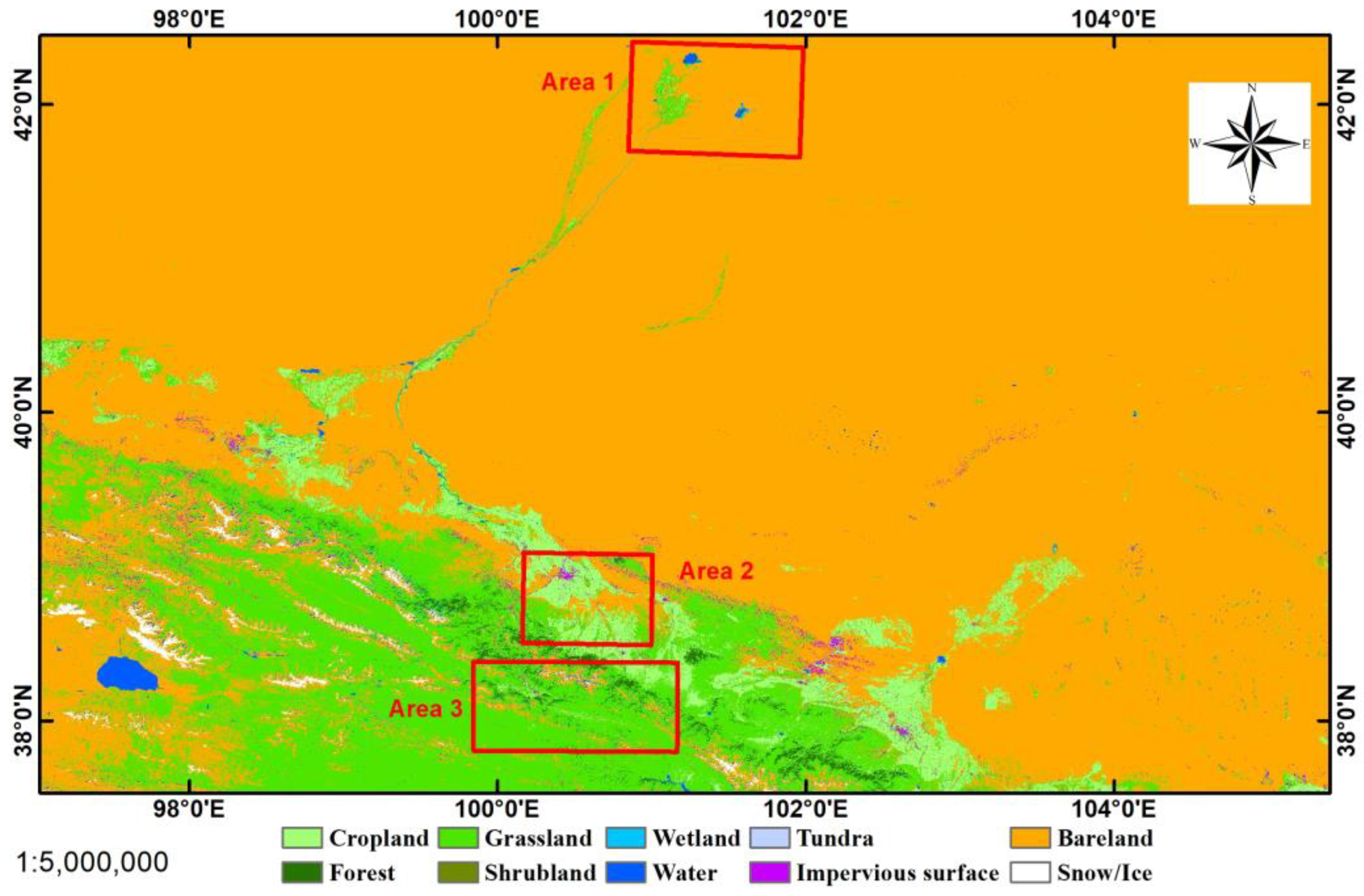
2.3. Experimental Area

To obtain accurate downscaled LST, three experimental areas were chosen to discuss how to select the optimal variables for different land cover types. Figure 1 illustrates the geographical location of the experimental area. The base map is based on the 30 m resolution global land cover maps [61] released by Tsinghua University in 2017. Experimental areas 1 to 3 (hereafter termed A1, A2, and A3) are located near the downstream, midstream, and upstream of Heihe River Basin in Gansu Province, China. The main land cover types are bareland, cropland and bareland, and grassland and forest for A1, A2, and A3, respectively.

2.4. Ground Measurements

In order to assess the precision of the downscaled LST, ground measurements were obtained from 21 sites representing various land cover types. In situ measurements can be downloaded from the National Tibetan Plateau/Third Pole Environment Data Center (TPDC). The ground measurements can be used to validate the performance of the machine learning algorithms in spatial downscaling of MODIS LST with multivariables. The basic information about the in situ site is shown in

Table 2. The basic information about the in situ site.

Experimental Area	Site	Name	Latitude	Longitude	Land Cover
A1	HYL	HuYangLin	41.993	101.124	populus forest
	HHL	HunHeLin	41.990	101.133	populus & tamarix
	LD	LuoDi	41.999	101.133	bareland
	NT	NongTian	42.005	101.134	grassland
	SDQ	SiDaoQiao	42.001	101.137	tamarix
	HM	HuangMo	42.1135	100.987	desert steppe
A2	GB	Gebi	38.915	100.304	gobi desert
	SSW	ShenShaWo	38.789	100.493	sand dune
	JCHM	JiChangHuangMo	38.778	100.697	desert steppe
	SD	ShiDi	38.975	100.446	reed wetland
	CJZ	ChaoJiZhan	38.855	100.372	corn
	YG	YaoGan	38.827	100.476	grassland
	HZZ	HuaZhaiZi	38.766	100.320	desert steppe
A3	ArouCJZ	Arou ChaoJiZhan	38.047	100.464	alpine meadow
	ArouYangpo	ArouYangpo	38.089	100.520
	ArouYinpo	ArouYinpo	37.984	100.411
	EB	EBao	37.949	100.915
	HZS	HuangZangSi	38.225	100.192	wheat
	HCG	HuangCaoGou	38.003	100.731	alpine meadow
	YK	YaKou	38.014	100.242
	DSL	DaShaLong	38.840	98.941	marsh

.

The in situ LSTs were estimated from the surface longwave upward/downward radiation measured by the Kipp & Zonen CNR1/CNR4 net radiometer using the following equation [62,63,64]:

$$T_s={\left[\left(F^{\uparrow }-\left(1-{\epsilon }_b\right)F^{\downarrow }\right)/\left({\epsilon }_b\sigma \right)\right]}^{0.25}$$

(4)

where $T_s$ is the LST, $F^{\uparrow } \mathrm{and} F^{\downarrow }$ are the surface upward longwave radiation and atmospheric downward longwave radiation, respectively, ${\epsilon }_b$ is the broadband emissivity (BBE), σ is the Stefan–Boltzmann constant (5.67 × 10⁻⁸ Wm⁻² K⁻⁴). The BBE was extracted from the Global LAnd Surface Satellite (GLASS) BBE product [65].

3. Results and Analysis

This section uses simulated coarse spatial resolution LST, and the MODIS LST product to discuss how to select the downscaling factors in different research areas. The potential for enhancing the accuracy of downscaled LST through incorporating slope and aspect variables is also discussed. The downscaling factors were divided into four categories to explore the influence of various downscaling factors on the LST downscaling in different experimental areas.

3.1. Downscaling Results of Simulated Coarse LST

First, the coarse spatial resolution LST and downscaling factors used in this section were obtained by resampling the original 30 m Landsat LST to 960 m using bilinear interpolation. Next, after combining the downscaling model established by the XGBoost and RF algorithm with the fine spatial resolution downscaling factors, an LST with a spatial resolution of 30 m can be acquired. Finally, the original 30 m Landsat LSTs were used to evaluate the performance of different downscaling factors through three evaluation indicators: average error (bias), mean absolute error (MAE), and root mean square error (RMSE).

Figure 2 presents the importance scores of independent variables for the RF model across all research dates in three areas. According to this ranking of importance, the fourth category downscaling factors were selected for LST downscaling. As demonstrated in Figure 2, the independent variable importance scores for the RF model demonstrate variability across disparate experimental domains. Consequently, it can be deduced that the same combination of downscaling factors will exert divergent effects on the LST downscaling results in different experimental domains. Furthermore, the presence of clouds has been demonstrated to engender discrepancies in the downscaling factor samples of disparate land cover types. This, in turn, gives rise to variations in the significance of downscaling factors on different days within the same experimental area. Following a comprehensive consideration of the results obtained from all images, the downscaling factors ${\rho }_{swir1}$, ${\rho }_{swir2}$, SAVI, NDSI, NMDI, NDDI, MNDWI, NDBI, and DEM, were selected for A1, whereas ${\rho }_b$, ${\rho }_g$, ${\rho }_r$, ${\rho }_{nir}$, ${\rho }_{swir1}$, ${\rho }_{swir2}$, NDVI, NDBI, and DEM were selected for A2, and ${\rho }_{nir}$, ${\rho }_{swir1}$, ${\rho }_{swir2}$, NDVI, NDBI, NDDI, MNDWI, NDBI, and DEM were selected for A3.

It can be seen from Figure 2 that slope and aspect are of low importance in different experimental areas, which should be excluded in theory. However, in order to show that the change of LST downscaling results is not due to the influence of slope and aspect, slope and aspect are finally added on the basis of the above selected downscaling factors.

The evaluation results of downscaled LST using XGBoost and four categories of downscaling factors are shown in Figure 3, whereas the evaluation results for RF are shown in Figure 4. For A1, the average values of MAEs of downscaled LST using XGBoost and four categories of downscaling factors were 1.14 K, 1.07 K, 1.05 K, and 1.01 K, and the average values of biases (RMSEs) were −0.34 (1.56) K, −0.33 (1.47) K, −0.32 (1.46) K, and −0.32 (1.41) K. For A2, the average values of MAEs of downscaled LST using XGBoost and four categories of downscaling factors were 1.65 K,1.60 K, 1.58 K, and 1.61 K, the average values of biases were −0.20 K, −0.44 K, −0.32 K, and −0.36 K, and the average values of RMSEs were 2.18 K, 2.13 K, 2.11 K, and 2.13 K. For A3, the performance of V2 in LST downscaling was slightly better than the other three categories of downscaling factors, and the performance of V4, V3, and V1 decreased in that order. The average values were 2.76 K, 2.43 K, 2.53 K, and 2.51 K for MAE, 1.01 K, 0.41 K, 0.74 K, and 0.64 K for bias, and 3.69 K, 3.28 K, 3.44 K, and 3.42 K for RMSE, respectively for the downscaled LST using XGBoost and V1, V2, V3, and V4. The results of the LST downscaling based on the RF algorithm are essentially in line with those of the XGBoost algorithm, with the differences between the three evaluation indicators all within 0.2 K.

After removing the slope and aspect factors from the above downscaling factors, the downscaled LST based on four categories of downscaling factors performs differently in three experimental areas. There is an approximate 0.3 K, 0.2 K, and 0.2 K decrease in bias, MAE, and RMSE for experimental area 1 and 2, respectively. In experimental area 3, bias increased by approximately 0.2 K, and RMSE increased by about 0.1 K, while MAE remained almost unchanged. The results of the LST downscaling derived using the RF algorithm are in close alignment with those obtained by the XGBoost algorithm.

In general, the four categories of downscaling factors performed similarly in the three experimental areas, with the exceptions that the accuracy of the first category of downscaling factors was poor on certain dates, and the differences in the RMSE averages of the other three categories of downscaling factors in all experimental areas were less than 0.4 K. Increasing the variable in the downscaling factor does not yield a substantial enhancement in the accuracy of LST downscaling. The downscaling factors of different combinations of vegetation indices and topographic parameters have good performance in different experimental areas. Therefore, the second category of downscaling factor with fewer input parameters can be selected as the downscaling factor. This category of downscaling factor can obtain high-precision LST in different experimental areas, and different vegetation indices and topographic parameters can be easily obtained.

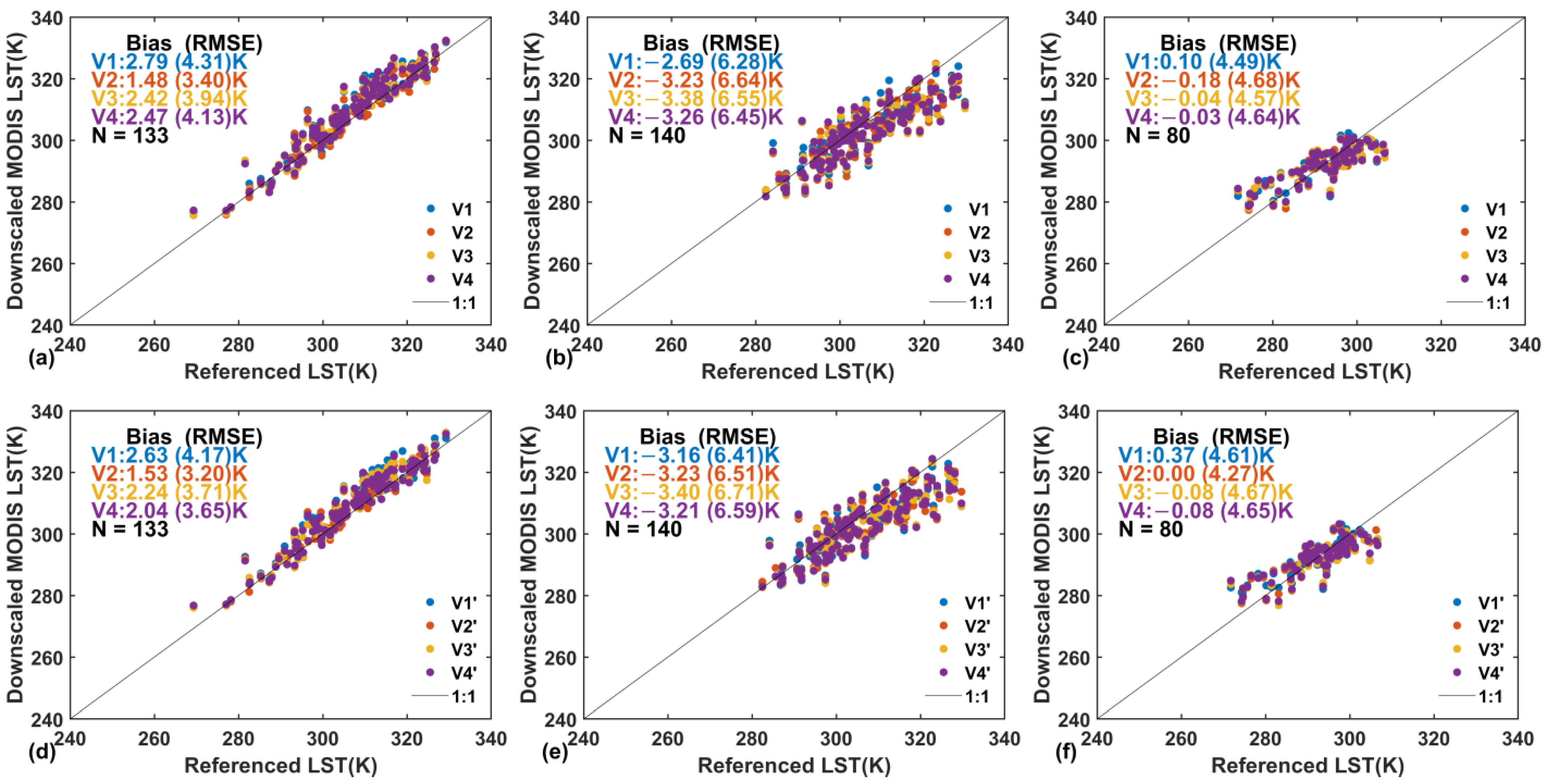
3.2. Downscaling Results of MODIS LST

In this section, XGBoost and RF are used to downscale MODIS LST, and the differences of four kinds of downscaling factors are analyzed. Firstly, MOD11_L2 LST and MOD09GA are used as the input data of the downscaling model, and then the downscaling model is established using two machine learning algorithms. Finally, the fine spatial resolution downscaling factor calculated by Landsat 8 data is inputted to obtain LST with 30 m spatial resolution. As illustrated in Figure 5 and Figure 6, the validation results of the downscaled MODIS LST using two different algorithms are demonstrated.

For A1, the performance of the second downscaling factor was slightly better than that of the other three when slope and aspect were not included in the downscaling factors. The bias (RMSE) of LST downscaled using the XGBoost and RF algorithms and V2′ is 1.53 (3.20) K and 1.81 (3.33) K, respectively. The bias (RMSE) of LST downscaled using the other three factors ranges from 2.04 (3.65) K to 2.63 (4.17) K for the XGBoost algorithm and from 2.49 (3.93) K to 2.64 (4.08) K for the RF algorithm. When slope and aspect were added to the downscaling factors, the accuracy of the two algorithms decreased to varying degrees. The XGBoost algorithm had a bias (RMSE) ranging from 1.48 (3.40) K to 2.79 (4.31) K, whereas the RF algorithm had a bias (RMSE) ranging from 1.73 (3.39) K to 2.79 (4.15) K.

For A2, it is evident that when slope and aspect were not included among the downscaling factors, there was no discernible change in the bias and RMSE. The bias (RMSE) of MODIS LST downscaled using the XGBoost algorithm ranged from −3.16 (6.41) K to −3.40 (6.71) K, whereas the bias (RMSE) of the RF algorithm ranged from −2.51 (6.19) K to −2.84 (6.37) K. When slope and aspect were added to the downscaling factors, the XGBoost algorithm had a bias (RMSE) ranging from −2.69 (6.28) K to −3.38 (6.64) K, and the RF algorithm had a bias (RMSE) ranging from −2.21 (6.16) K to −2.74 (6.54) K.

For A3, the XGBoost algorithm demonstrated a marginally superior degree of accuracy in comparison to the RF algorithm. Prior to the incorporation of slope and aspect as downscaling factors, the bias of the MODIS LST downscaled by the XGBoost (RF) algorithm was 0.37 (0.23) K, 0.00 (−0.17) K, −0.08 (−0.09) K, and −0.08 (−0.14) K for V1′, V2′, V3′, and V4′, whereas the corresponding RMSE was 4.61 (4.74), 4.27 (4.65), 4.67 (4.80), and 4.65 (4.79) K, respectively. Once slope and aspect were added to the downscaling factors, the bias of MODIS LST downscaled by the XGBoost (RF) algorithm was 0.10 (0.16) K, −0.18 (−0.16) K, −0.04 (−0.19) K, and −0.03 (−0.32) K for V1, V2, V3, and V4, respectively. The corresponding RMSEs were 4.49 K, 4.68 K, 4.57 K, and 4.64 K for the XGBoost algorithm, whereas the RMSEs were 4.69 K, 4.67 K, 4.83 K, and 4.93 K for the RF algorithm.

In conclusion, the second kind of downscaling factor is recommended as the input parameter of downscaling based on the in situ validation results of simulation and MODIS data. Despite the absence of a readily discernible discrepancy, the in situ validation accuracy of downscaled LST in the majority of experimental areas appears to be weakened by the incorporation of slope and aspect into downscaling factors. This observation is corroborated by the results of simulation data. Consequently, it is recommended that slope and aspect be considered in conjunction with other downscaling factors to optimize the accuracy of LST downscaling in mountainous regions.

4. Discussion

4.1. Possible Reasons for the Poor Performance of the Downscale Results

There are many outliers with large errors in Figure 3 and Figure 4. We selected one image in each experimental area to analyze the potential factors contributing to the suboptimal performance of the downscaling results. As can be seen from the pseudo-color composite image in Figure 7, the poor performance in experimental area 1 is due to the presence of thin clouds and debris clouds that were not detected. The LST around the cloud is estimated much higher than it should be, and it is difficult to establish a reasonable relationship between LST and downscaling factors because there are not enough training data due to the presence of clouds. The anomalies of experimental areas 2 and 3 mainly occur in regions covered by ice and snow, and their deviations are greater than 10 K. The downscaling factors containing LSR perform poorly in ice and snow regions, and the downscaling factors only using the combination of LSR and topographic factors have the worst results. Therefore, it can be inferred that the LSR is not suitable for LST downscaling in icy and snowy regions, while vegetation indices can obtain more accurate LSTs when used as a downscaling factor.

To illustrate our findings, Figure 8 presents an analysis of temporal error trends and seasonal patterns of downscaled LST for A3. The downscaled LST was obtained using XGBoost and V1 as downscaling variables. Panel (a) depicts the temporal bias associated with ice/snow-covered, non-vegetated, and vegetated land surfaces, while panels (b) through (d) illustrate the seasonal bias for these three types of land surfaces. The bias observed in non-vegetated land surfaces ranges from −0.95 K to 1.05 K, with a median value of −0.15 K. In contrast, the bias for vegetated land surfaces spans from −0.68 K to 1.27 K, exhibiting a median value of −0.17 K. Compared with statistics from non-ice/snow areas, the statistics from ice/snow areas reveal a greater deviation in all seasons, particularly in spring and winter, when land surface reflectance and terrain elements were employed as a downscaling factor.

The poor performance of the downscale results could be explained by the slope and aspect. As shown in Figure 9, after adding the slope and aspect, the downscaled LST over vegetation in experimental area 1 changed from slightly overestimated to seriously underestimated, with the bias (RMSE) changing from −0.56 (2.24) K to −1.34 (3.20) K. After slope and aspect were added, the LST was found to be underestimated in certain regions of experimental area 2, especially in the desert. The bias and RMSE of LST decreased from −0.56 K to −1.44 K and from 2.24 K to 2. 78 K, respectively. In experimental area 3, adding slope and aspect improved the accuracy of LST downscaling. However, compared with other experimental areas, the accuracy of LST downscaling is still low in mountainous areas covered with ice and snow.

In general, the addition of slope and aspect during LST downscaling on most dates caused the LST to be underestimated to varying degrees. Adding slope and aspect reduces the accuracy of LST downscaling in the first two experimental areas and improves it in the third. Therefore, when downscaling LST in mountainous areas with significant topographic relief, DEM, slope, and aspect can be incorporated alongside other factors to enhance the accuracy of the downscaling process. In areas with minimal topographic relief, such as high-altitude regions with minor slope changes, downscaled LST can be obtained with high accuracy using only DEM and other downscaling factors.

The larger biases in Figure 5 and Figure 6 can be explained by the following two reasons. (1) Issues of the MODIS LST product. The MOD11 product is subject to uncertainty due to the limitations in the emissivity of the MODIS 31 and 32 bands, which are calculated using classification-based methods. The deviations of the individual validation points in experimental area 2 are between −4.69 K and −2.27 K [53] and between −2.62 K and −0.94 K [54]. (2) Challenges of temperature-based validation. There are numerous significant considerations to make in the context of temperature-based validation. These encompass the precision of ground measurements, the spatial representativeness of LST validation sites relative to the scale of satellite pixels, and the discrepancies in viewing angles between TIR field radiometers and satellite sensors [66,67]. For example, the ArouCJZ and SDQ sites showed greater spatial heterogeneity during the daytime [68], which may render them unsuitable for temperature-based validation.

4.2. Compared with LST Downscaled Using GWR

In this section, the GWR algorithm is used to downscale MODIS LST, and the differences of four kinds of downscaling factors are analyzed. As shown in

Table 3. The validation result of the MODIS LST downscaled using the GWR algorithm.

Experimental Area	Downscaling Factors	Bias (K)	RMSE (K)
A1	V1/V1′	−3.86/−0.19	8.78/4.11
	V2/V2′	−4.52/−0.33	8.75/4.17
	V3/V3′	−4.53/0.07	10.46/5.87
	V4/V4′	−10.02/−4.82	22.79/23.63
A2	V1/V1′	−3.02/−3.40	7.73/6.90
	V2/V2′	−3.59/−3.87	7.16/6.98
	V3/V3′	−3.71/−3.62	7.13/6.97
	V4/V4′	−3.22/−3.68	11.23/11.62
A3	V1/V1′	−0.82/−0.82	4.59/4.69
	V2/V2′	−0.48/−0.44	4.02/4.19
	V3/V3′	0.32/0.53	6.48/7.17
	V4/V4′	−1.24/−1.03	7.85/8.03

, the performance of the fourth downscaling factor in the GWR algorithm differs significantly from that of the other three factors, exhibiting greater bias and RMSE. Removing slope and aspect from the downscaling factors significantly improved the accuracy of the GWR algorithm in the experimental area 1, whereas there was only a slight decrease in uncertainty in the experimental area 2. After adding slope and aspect, the changes to the GWR algorithm in the experimental area 3 were less obvious, with only a slight decrease in uncertainty.

The GWR algorithm is less accurate than the XGBoost and RF algorithms in all three experimental areas. The performance of the four categories of downscaling factors in the machine learning algorithm is generally consistent. There are no significant differences whether or not the downscaling factors include slope and aspect. The first three categories of downscaling factors in the GWR algorithm are relatively consistent in terms of accuracy, while the fourth category has lower accuracy. The fourth category of downscaling factors is not suitable for LST downscaling using the GWR algorithm. This is because machine-learning-based downscaling methods establish non-linear regression relationships globally, whereas the GWR model establishes linear regression relationships locally. Consequently, the fourth category of downscaling factors performs poorly in the GWR algorithm.

4.3. Comparison with Existing Studies

Table 4. The evaluation result of the downscaled LST in existing studies.

Reference	Algorithm	Downscaling Factors	Target Resolution	Evaluation	Metric (K)
[33]	RF*	Blue, Green, Red, NIR, SWIR1, SWIR2, BSI, MSAVI, NDBI, NDDI, NDVI, NDWI, MNDWI, OSAVI, SAVI, IBI, IVI, UI, DEM, slope, aspect, LC	100 m	Landsat LST	MAE: 0.70~1.45 RMSE: 0.94~2.07
[39]	GWR	NDVI, DEM	90 m	ASTER LST	MAE: 1.28~1.86 RMSE: 2.7~3.6
[40]	GWR RF	NDBI, NDVI, DEM, slope	30 m	Landsat LST	MAE: 0.71~0.77 RMSE: 0.94~1.19 MAE: 0.88~3.30 RMSE: 1.15~4.23
[46]	RF	Blue, Green, Red, NIR, SWIR1, SWIR2, DEM, solar incidence angle, sky-view factor, LC	240 m	Landsat LST	RMSE: 0.98~1.45
[48]	RF	NDVI, DEM	250 m	Landsat LST	MAE: 1.7 RMSE: 2.2
[49]	RF	Blue, Green, Red, NIR, SWIR1, SWIR2, DEM, aspect, slope, hill-shade, NDVI, SAVI, NDDI, NMDI, MNDWI, NDBI, LC	90 m	ASTER LST	RMSE: 2.10~3.99
[50]	RF*	Blue, Green, Red, NIR, RE1, RE2, RE3, NNIR, SWIR1, SWIR2, Water vapor, DEM, aspect, slope, NDVI, SAVI, EVI, FVC, BSI, NDBI, NDWI, NMDI, NDMI	100 m	Landsat LST	Bias: −1.21~0.72 RMSE: 2.52~3.16
[69]	RF	SAVI, NMDI, MNDWI, NDBI, NDDI, LC	500 m	In situ data	Bias: −2.64~2.45 RMSE: 0.91

NIR: Near Infrared, RE1: Red Edge 1, RE2: Red Edge 2, RE3: Red Edge 3, NNIR: Narrow Near Infrared, SWIR1: Shortwave Infrared 1, SWIR2: Shortwave Infrared 2, LC: land cover, BSI: Bare soil index, EVI: Enhanced Vegetation Index, FVC: Fraction Vegetation Cover, IBI: Index-based built-up index, IVI: Index-based vegetation index, MNDWI: Modified normalized difference water index, MSAVI: Modified soil adjusted vegetation index, NDBI: Normalized difference built-up index, NDDI: Normalized difference drought index, NDVI: Normalized difference vegetation index, NDMI: Normalized Difference Moisture Index, NDWI: Normalized difference water index, NMDI: normalized multiband drought index, OSAVI: Optimal soil adjusted vegetation index, SAVI: Soil adjusted vegetation index, UI: Urban index. RF* denotes the selection of features derived from all available downscaling factors.

shows the evaluation results of LST downscaled using RF and GWR algorithms, as reported in various existing studies. Four studies employed fewer than six downscaling factors, while the remaining four studies utilized more than ten downscaling factors. Notably, Tang et al. [33] and Njuki et al. [50] implemented various strategies to identify the optimal downscaling factor from among multiple downscaling factors. When using ASTER LST as evaluation data, the RMSE between the referenced LST and the predicted LST exceeded 2.10 K. When RF was used for downscaling, the MAE between Landsat LST and downscaled LST ranged from 0.70 K to 1.70 K, while RMSE exhibits large fluctuations, with values ranging from 0.94 K to 4.23 K in different experimental areas. In this study, four categories of downscaling factors were employed for the LST downscaling, and Landsat LST was used for evaluation. The results yielded average MAE values ranging from 1.54 K to 1.86 K, average RMSE values ranging from 2.13 K to 2.50 K, and average bias values ranging from −0.18 K to 0.31 K. From the perspective of cross-validation, the accuracy of the downscaling algorithm employed in this study is consistent with that utilized in previous studies. With regards to the validation results employing in situ data, the performance of the RF algorithm demonstrates significant fluctuations across diverse land cover types. When the land surface is covered by maize or orchards, the bias approaches a value of zero, whereas on wetland and desert surfaces, the bias exceeds 2.45 K [69]. Based on the validation results of Yang et al. [69] in experimental area 2, the MOD11 product is underestimated by over 5.0 K in Gobi and desert, and the absolute bias of wetland, orchard, and wilderness is also greater than 1.80 K. This might help clarify why our downscaling results did not perform as well as expected.

4.4. Possible Improvements

The radiative balance of the surface is influenced by the angle of solar illumination, which depends on the slope and aspect, as well as the elevation and azimuth of the sun. Previous studies indicate that the substantial impact of orography on LST can be alleviated through two primary approaches: (1) the integration of data pertaining to solar incidence angles and sky-view factors into machine learning models [46] and (2) the implementation of a topographic-adjusted scheme for LST prior to the training of machine learning models, which serves to diminish the influences of terrain self-shadowing and cast-shadowing [70,71].

Given that not all variables within the model significantly enhance its performance, the removal of those variables that detract from predictive accuracy may lead to improved performance and a more streamlined model. For instance, there is a strong correlation between LSR in different bands and between different vegetation indices. Consequently, it is essential to minimize the number of variables while ensuring that the model’s performance either improves or remains stable. The selection of optimal features can be achieved through various methodologies, including support vector machine [51], principal component analysis [72], and minimum redundancy maximum relevance [73].

5. Conclusions

First, we evaluated the performance of four categories of downscaling factor in three experimental areas using the XGBoost, RF, and GWR algorithms, and simulated coarse spatial resolution LST and the MODIS LST product. The influence of slope and aspect on LST downscaling was then analyzed in detail. Finally, the performance of various downscaling models and factors was validated using in situ data. The following is a summary of the major findings:

(1)

Increasing the variables in the downscaling factors cannot effectively improve the downscaling accuracy of LST. In certain experimental regions, the incorporation of slope and aspect may enhance the precision of LST downscaling.

(2)

The combination of multiple vegetation indices and terrain elements can obtain fine spatial resolution LSTs with high accuracy in different experimental areas. The LSR is not suitable for LST downscaling in ice and snow regions.

(3)

The validation results demonstrate that the XGBoost and RF algorithms are more appropriate for LST downscaling than the GWR model.

Despite the capacity to acquire high-spatial LST through the utilization of a downscaling algorithm, the effectiveness of this method is dependent on the existence of clouds. In future work, the incorporation of the spatio-temporal fusion algorithm and all-weather LST into the algorithm may be considered, with a view to enhancing its efficacy in relation to the urban heat island and other fields.

References

1. Mannstein, H. Surface Energy Budget, Surface Temperature and Thermal Inertia. In Remote Sensing Applications in Meteorology and Climatology; Mannstein, H., Ed.; Springer: Dordrecht, The Netherlands, 1987; pp. 391–410. [Google Scholar]
2. Wan, Z.; Dozier, J. A generalized split-window algorithm for retrieving land-surface temperature from space. IEEE Trans. Geosci. Remote Sens. 1996, 34, 892–905. [Google Scholar]
3. Cheng, J.; Liang, S.; Wang, J.; Li, X. A Stepwise Refining Algorithm of Temperature and Emissivity Separation for Hyperspectral Thermal Infrared Data. IEEE Trans. Geosci. Remote Sens. 2010, 48, 1588–1597. [Google Scholar] [CrossRef]
4. Zhou, S.; Cheng, J.; Shi, J. A Physical-Based Framework for Estimating the Hourly All-Weather Land Surface Temperature by Synchronizing Geostationary Satellite Observations and Land Surface Model Simulations. IEEE Trans. Geosci. Remote Sens. 2022, 60, 1–22. [Google Scholar] [CrossRef]
5. Valor, E.; Caselles, V. Mapping land surface emissivity from NDVI: Application to European, African, and South American areas. Remote Sens. Environ. 1996, 57, 167–184. [Google Scholar]
6. Zhang, Y.Z.; Cheng, J. Spatio-Temporal Analysis of Urban Heat Island Using Multisource Remote Sensing Data: A Case Study in Hangzhou, China. IEEE J. Sel. Top. Appl. Earth Obs. Remote Sens. 2019, 12, 3317–3326. [Google Scholar] [CrossRef]
7. Cheng, J.; Kustas, W. Using Very High Resolution Thermal Infrared Imagery for More Accurate Determination of the Impact of Land Cover Differences on Evapotranspiration in an Irrigated Agricultural Area. Remote Sens. 2019, 11, 613. [Google Scholar] [CrossRef]
8. Liu, X.; Tang, B.-H.; Li, Z.-L.; Zhou, C.; Wu, W.; Rasmussen, M.O. An improved method for separating soil and vegetation component temperatures based on diurnal temperature cycle model and spatial correlation. Remote Sens. Environ. 2020, 248, 111979. [Google Scholar] [CrossRef]
9. Dong, L.; Tang, S.; Wang, F.; Cosh, M.; Li, X.; Min, M. Inversion and Validation of FY-4A Official Land Surface Temperature Product. Remote Sens. 2023, 15, 2437. [Google Scholar] [CrossRef]
10. Meng, X.; Liu, W.; Cheng, J.; Guo, H.; Yao, B. Estimating Hourly Land Surface Temperature From FY-4A AGRI Using an Explicitly Emissivity-Dependent Split-Window Algorithm. IEEE J. Sel. Top. Appl. Earth Obs. Remote Sens. 2023, 16, 5474–5487. [Google Scholar] [CrossRef]
11. Zhao, W.; Yang, Y.; Yang, M. An Improved Annual Temperature Cycle Model with the Consideration of Vegetation Change. IEEE Geosci. Remote Sens. Lett. 2022, 19, 1–5. [Google Scholar] [CrossRef]
12. Zheng, X.; Li, Z.-L.; Wang, T.; Huang, H.; Nerry, F. Determination of global land surface temperature using data from only five selected thermal infrared channels: Method extension and accuracy assessment. Remote Sens. Environ. 2022, 268, 112774. [Google Scholar] [CrossRef]
13. Wang, M.; Li, M.; Zhang, Z.; Hu, T.; He, G.; Zhang, Z.; Wang, G.; Li, H.; Tan, J.; Liu, X. Land Surface Temperature Retrieval From Landsat 9 TIRS-2 Data Using Radiance-Based Split-Window Algorithm. IEEE J. Sel. Top. Appl. Earth Obs. Remote Sens. 2023, 16, 1100–1112. [Google Scholar] [CrossRef]
14. Gao, J.; Sun, H.; Xu, Z.; Zhang, T.; Xu, H.; Wu, D.; Zhao, X. CPMF: An Integrated Technology for Generating 30-m, All-Weather Land Surface Temperature by Coupling Physical Model, Machine Learning, and Spatiotemporal Fusion Model. IEEE Trans. Geosci. Remote Sens. 2024, 62, 1–16. [Google Scholar] [CrossRef]
15. Prigent, C.; Jimenez, C.; Aires, F. Toward “all weather,” long record, and real-time land surface temperature retrievals from microwave satellite observations. J. Geophys. Res. Atmos. 2016, 121, 5699–5717. [Google Scholar] [CrossRef]
16. Wu, P.; Su, Y.; Duan, S.-b.; Li, X.; Yang, H.; Zeng, C.; Ma, X.; Wu, Y.; Shen, H. A two-step deep learning framework for mapping gapless all-weather land surface temperature using thermal infrared and passive microwave data. Remote Sens. Environ. 2022, 277, 113070. [Google Scholar] [CrossRef]
17. Sepulcre-Canto, G.; Zarco-Tejada, P.J.; Jimenez-Munoz, J.C.; Sobrino, J.A.; de Miguel, E.; Villalobos, F.J. Detection of water stress in an olive orchard with thermal remote sensing imagery. Agric. For. Meteorol. 2006, 136, 31–44. [Google Scholar] [CrossRef]
18. Sepulcre-Canto, G.; Zarco-Tejada, P.J.; Jimenez-Munoz, J.C.; Sobrino, J.A.; Soriano, M.A.; Fereres, E.; Vega, V.; Pastor, M. Monitoring yield and fruit quality parameters in open-canopy tree crops under water stress. Implications for ASTER. Remote Sens. Environ. 2007, 107, 455–470. [Google Scholar] [CrossRef]
19. Zhukov, B.; Lorenz, E.; Oertel, D.; Wooster, M.; Roberts, G. Spaceborne detection and characterization of fires during the bi-spectral infrared detection (BIRD) experimental small satellite mission (2001–2004). Remote Sens. Environ. 2006, 100, 29–51. [Google Scholar]
20. Sobrino, J.A.; Gómez, M.; Jiménez-Muñoz, J.C.; Olioso, A.; Chehbouni, G. A simple algorithm to estimate evapotranspiration from DAIS data: Application to the DAISEX campaigns. J. Hydrol. 2005, 315, 117–125. [Google Scholar] [CrossRef]
21. Sobrino, J.A.; Jimenez-Munoz, J.C.; Soria, G.; Gomez, M.; Ortiz, A.B.; Romaguera, M.; Zaragoza, M.; Julien, Y.; Cuenca, J.; Atitar, M.; et al. Thermal remote sensing in the framework of the SEN2FLEX project: Field measurements, airborne data and applications. Int. J. Remote Sens. 2008, 29, 4961–4991. [Google Scholar] [CrossRef]
22. Zhan, W.F.; Chen, Y.H.; Zhou, J.; Li, J.; Liu, W.Y. Sharpening Thermal Imageries: A Generalized Theoretical Framework From an Assimilation Perspective. IEEE Trans. Geosci. Remote Sens. 2011, 49, 773–789. [Google Scholar]
23. Yang, B.; Liu, H.; Kang, E.L.; Shu, S.; Xu, M.; Wu, B.; Beck, R.A.; Hinkel, K.M.; Yu, B. Spatio-temporal Cokriging method for assimilating and downscaling multi-scale remote sensing data. Remote Sens. Environ. 2021, 255, 112190. [Google Scholar] [CrossRef]
24. Zhan, W.; Chen, Y.; Wang, J.; Zhou, J.; Quan, J.; Liu, W.; Li, J. Downscaling land surface temperatures with multi-spectral and multi-resolution images. Int. J. Appl. Earth Obs. Geoinf. 2012, 18, 23–36. [Google Scholar] [CrossRef]
25. Zhukov, B.; Oertel, D.; Lanzl, F.; Reinhackel, G. Unmixing-based multisensor multiresolution image fusion. IEEE Trans. Geosci. Remote Sens. 1999, 37, 1212–1226. [Google Scholar]
26. Liu, D.S.; Pu, R.L. Downscaling thermal infrared radiance for subpixel land surface temperature retrieval. Sensors 2008, 8, 2695–2706. [Google Scholar] [CrossRef]
27. Li, M.; Guo, S.; Chen, J.; Chang, Y.; Sun, L.; Zhao, L.; Li, X.; Yao, H. Stability Analysis of Unmixing-Based Spatiotemporal Fusion Model: A Case of Land Surface Temperature Product Downscaling. Remote Sens. 2023, 15, 901. [Google Scholar] [CrossRef]
28. Agam, N.; Kustas, W.P.; Anderson, M.C.; Li, F.Q.; Neale, C.M.U. A vegetation index based technique for spatial sharpening of thermal imagery. Remote Sens. Environ. 2007, 107, 545–558. [Google Scholar]
29. Dominguez, A.; Kleissl, J.; Luvall, J.C.; Rickman, D.L. High-resolution urban thermal sharpener (HUTS). Remote Sens. Environ. 2011, 115, 1772–1780. [Google Scholar]
30. Wang, Q.M.; Shi, W.Z.; Atkinson, P.M. Area-to-point regression kriging for pan-sharpening. ISPRS J. Photogramm. Remote Sens. 2016, 114, 151–165. [Google Scholar]
31. Peng, Y.; Li, W.; Luo, X.; Li, H. A Geographically and Temporally Weighted Regression Model for Spatial Downscaling of MODIS Land Surface Temperatures Over Urban Heterogeneous Regions. IEEE Trans. Geosci. Remote Sens. 2019, 57, 5012–5027. [Google Scholar] [CrossRef]
32. Zhang, Q.; Wang, N.; Cheng, J.; Xu, S. A Stepwise Downscaling Method for Generating High-Resolution Land Surface Temperature from AMSR-E Data. IEEE J. Sel. Top. Appl. Earth Obs. Remote Sens. 2020, 13, 5669–5681. [Google Scholar] [CrossRef]
33. Tang, K.; Zhu, H.; Ni, P. Spatial Downscaling of Land Surface Temperature over Heterogeneous Regions Using Random Forest Regression Considering Spatial Features. Remote Sens. 2021, 13, 3645. [Google Scholar] [CrossRef]
34. Kustas, W.P.; Norman, J.M.; Anderson, M.C.; French, A.N. Estimating subpixel surface temperatures and energy fluxes from the vegetation index–radiometric temperature relationship. Remote Sens. Environ. 2003, 85, 429–440. [Google Scholar] [CrossRef]
35. Agam, N.; Kustas, W.P.; Anderson, M.C.; Li, F.; Colaizzi, P.D. Utility of thermal sharpening over Texas high plains irrigated agricultural fields. J. Geophys. Res. 2007, 112, D19. [Google Scholar] [CrossRef]
36. Essa, W.; Verbeiren, B.; van der Kwast, J.; Batelaan, O. Improved DisTrad for Downscaling Thermal MODIS Imagery over Urban Areas. Remote Sens. 2017, 9, 1243. [Google Scholar] [CrossRef]
37. Yang, Y.; Li, X.; Pan, X.; Zhang, Y.; Cao, C. Downscaling Land Surface Temperature in Complex Regions by Using Multiple Scale Factors with Adaptive Thresholds. Sensors 2017, 17, 744. [Google Scholar] [CrossRef] [PubMed]
38. Ding, L.; Zhou, J.; Ma, J.; Zhu, X.; Wang, W.; Li, M. A Spatial Downscaling Approach for Land Surface Temperature by Considering Descriptor Weight. IEEE Geosci. Remote Sens. Lett. 2023, 20, 1–5. [Google Scholar] [CrossRef]
39. Duan, S.-B.; Li, Z.-L. Spatial Downscaling of MODIS Land Surface Temperatures Using Geographically Weighted Regression: Case Study in Northern China. IEEE Trans. Geosci. Remote Sens. 2016, 54, 6458–6469. [Google Scholar] [CrossRef]
40. Liang, M.; Zhang, L.; Wu, S.; Zhu, Y.; Dai, Z.; Wang, Y.; Qi, J.; Chen, Y.; Du, Z. A High-Resolution Land Surface Temperature Downscaling Method Based on Geographically Weighted Neural Network Regression. Remote Sens. 2023, 15, 1740. [Google Scholar] [CrossRef]
41. Chen, J.; Liu, X.; Tang, B.-H.; Xu, Y.; Fan, D.; Huang, L.; Ge, Z.; Zhang, Z.; Zhong, Y.; Yang, C. An Integrated Object- and Pixel-Based Residual Compensation Framework for Land Surface Temperature Downscaling. IEEE Trans. Geosci. Remote Sens. 2025, 63, 1–16. [Google Scholar] [CrossRef]
42. Dai, Q.; Yuan, C.; Dai, Y.; Li, Y.; Li, X.; Ni, K.; Xu, J.; Shu, X.; Yang, J. MoCoLSK: Modality-Conditioned High-Resolution Downscaling for Land Surface Temperature. IEEE Trans. Geosci. Remote Sens. 2025, 63, 1–17. [Google Scholar] [CrossRef]
43. Xia, H. Geographically Constrained Machine Learning-Based Kernel-Driven Method for Downscaling of All-Weather Land Surface Temperature. Remote Sens. 2025, 17, 1413. [Google Scholar] [CrossRef]
44. Guijun, Y.; Ruiliang, P.; Wenjiang, H.; Jihua, W.; Chunjiang, Z. A Novel Method to Estimate Subpixel Temperature by Fusing Solar-Reflective and Thermal-Infrared Remote-Sensing Data with an Artificial Neural Network. IEEE Trans. Geosci. Remote Sens. 2010, 48, 2170–2178. [Google Scholar] [CrossRef]
45. Yang, G.; Pu, R.; Zhao, C.; Huang, W.; Wang, J. Estimation of subpixel land surface temperature using an endmember index based technique: A case examination on ASTER and MODIS temperature products over a heterogeneous area. Remote Sens. Environ. 2011, 115, 1202–1219. [Google Scholar] [CrossRef]
46. Hutengs, C.; Vohland, M. Downscaling land surface temperatures at regional scales with random forest regression. Remote Sens. Environ. 2016, 178, 127–141. [Google Scholar] [CrossRef]
47. Li, W.; Ni, L.; Li, Z.-L.; Duan, S.-B.; Wu, H. Evaluation of Machine Learning Algorithms in Spatial Downscaling of MODIS Land Surface Temperature. IEEE J. Sel. Top. Appl. Earth Obs. Remote Sens. 2019, 12, 2299–2307. [Google Scholar] [CrossRef]
48. Bartkowiak, P.; Castelli, M.; Notarnicola, C. Downscaling Land Surface Temperature from MODIS Dataset with Random Forest Approach over Alpine Vegetated Areas. Remote Sens. 2019, 11, 1319. [Google Scholar] [CrossRef]
49. Wu, H.; Li, W. Downscaling Land Surface Temperatures Using a Random Forest Regression Model with Multitype Predictor Variables. IEEE Access 2019, 7, 21904–21916. [Google Scholar] [CrossRef]
50. Njuki, S.M.; Mannaerts, C.M.; Su, Z. An Improved Approach for Downscaling Coarse-Resolution Thermal Data by Minimizing the Spatial Averaging Biases in Random Forest. Remote Sens. 2020, 12, 3507. [Google Scholar] [CrossRef]
51. Ebrahimy, H.; Azadbakht, M. Downscaling MODIS land surface temperature over a heterogeneous area: An investigation of machine learning techniques, feature selection, and impacts of mixed pixels. Comput. Geosci. 2019, 124, 93–102. [Google Scholar] [CrossRef]
52. Rodriguez-Galiano, V.; Pardo-Iguzquiza, E.; Sanchez-Castillo, M.; Chica-Olmo, M.; Chica-Rivas, M. Downscaling Landsat 7 ETM+ thermal imagery using land surface temperature and NDVI images. Int. J. Appl. Earth Obs. Geoinf. 2012, 18, 515–527. [Google Scholar] [CrossRef]
53. Duan, S.-B.; Li, Z.-L.; Li, H.; Göttsche, F.-M.; Wu, H.; Zhao, W.; Leng, P.; Zhang, X.; Coll, C. Validation of Collection 6 MODIS land surface temperature product using in situ measurements. Remote Sens. Environ. 2019, 225, 16–29. [Google Scholar] [CrossRef]
54. Li, H.; Yang, Y.; Li, R.; Wang, H.; Cao, B.; Bian, Z.; Hu, T.; Du, Y.; Sun, L.; Liu, Q. Comparison of the MuSyQ and MODIS Collection 6 Land Surface Temperature Products Over Barren Surfaces in the Heihe River Basin, China. IEEE Trans. Geosci. Remote Sens. 2019, 57, 8081–8094. [Google Scholar] [CrossRef]
55. Vermote, E.; Justice, C.; Csiszar, I. Early evaluation of the VIIRS calibration, cloud mask and surface reflectance Earth data records. Remote Sens. Environ. 2014, 148, 134–145. [Google Scholar] [CrossRef]
56. Fujisada, H.; Urai, M.; Iwasaki, A. Technical Methodology for ASTER Global DEM. IEEE Trans. Geosci. Remote Sens. 2012, 50, 3725–3736. [Google Scholar] [CrossRef]
57. Vermote, E.; Justice, C.; Claverie, M.; Franch, B. Preliminary analysis of the performance of the Landsat 8/OLI land surface reflectance product. Remote Sens. Environ. 2016, 185, 46–56. [Google Scholar] [CrossRef]
58. Cheng, J.; Meng, X.; Dong, S.; Liang, S. Generating the 30-m land surface temperature product over continental China and USA from landsat 5/7/8 data. Sci. Remote Sens. 2021, 4, 100032. [Google Scholar] [CrossRef]
59. Meng, X.; Cheng, J. Evaluating Eight Global Reanalysis Products for Atmospheric Correction of Thermal Infrared Sensor—Application to Landsat 8 TIRS10 Data. Remote Sens. 2018, 10, 474. [Google Scholar] [CrossRef]
60. Meng, X.; Guo, H.; Cheng, J.; Yao, B. Can the ERA5 Reanalysis Product Improve the Atmospheric Correction Accuracy of Landsat Series Thermal Infrared Data? IEEE Geosci. Remote Sens. Lett. 2022, 19, 7506805. [Google Scholar] [CrossRef]
61. Gong, P.; Wang, J.; Yu, L.; Zhao, Y.; Zhao, Y.; Liang, L.; Niu, Z.; Huang, X.; Fu, H.; Liu, S.; et al. Finer resolution observation and monitoring of global land cover: First mapping results with Landsat TM and ETM+ data. Int. J. Remote Sens. 2013, 34, 2607–2654. [Google Scholar] [CrossRef]
62. Ma, J.; Zhou, J.; Göttsche, F.-M.; Wang, Z.; Wu, H.; Tang, W.; Li, M.; Liu, S. An atmospheric influence correction method for longwave radiation-based in-situ land surface temperature. Remote Sens. Environ. 2023, 293, 113611. [Google Scholar] [CrossRef]
63. Ye, X.; Ren, H.; Zhu, J.; Fan, W.; Qin, Q. Split-Window Algorithm for Land Surface Temperature Retrieval From Landsat-9 Remote Sensing Images. IEEE Geosci. Remote Sens. Lett. 2022, 19, 1–5. [Google Scholar] [CrossRef]
64. Zeng, Q.; Cheng, J.; Sun, H.; Dong, S. An integrated framework for estimating the hourly all-time cloudy-sky surface long-wave downward radiation for Fengyun-4A/AGRI. Remote Sens. Environ. 2024, 312, 114319. [Google Scholar] [CrossRef]
65. Cheng, J.; Liang, S. Estimating global land surface broadband thermal-infrared emissivity using advanced very high resolution radiometer optical data. Int. J. Digit. Earth 2013, 6, 34–49. [Google Scholar] [CrossRef]
66. Yu, Y.; Tarpley, D.; Privette, J.L.; Flynn, L.E.; Xu, H.; Chen, M.; Vinnikov, K.Y.; Sun, D.; Tian, Y. Validation of GOES-R Satellite Land Surface Temperature Algorithm Using SURFRAD Ground Measurements and Statistical Estimates of Error Properties. IEEE Trans. Geosci. Remote Sens. 2012, 50, 704–713. [Google Scholar] [CrossRef]
67. Coll, C.; Niclòs, R.; Puchades, J.; García-Santos, V.; Galve, J.M.; Pérez-Planells, L.; Valor, E.; Theocharous, E. Laboratory calibration and field measurement of land surface temperature and emissivity using thermal infrared multiband radiometers. Int. J. Appl. Earth Obs. Geoinf. 2019, 78, 227–239. [Google Scholar] [CrossRef]
68. Liu, W.; Shi, J.; Liang, S.; Zhou, S.; Cheng, J. Simultaneous retrieval of land surface temperature and emissivity from the FengYun-4A advanced geosynchronous radiation imager. Int. J. Digit. Earth 2022, 15, 198–225. [Google Scholar] [CrossRef]
69. Yang, Y.; Cao, C.; Pan, X.; Li, X.; Zhu, X. Downscaling Land Surface Temperature in an Arid Area by Using Multiple Remote Sensing Indices with Random Forest Regression. Remote Sens. 2017, 9, 789. [Google Scholar] [CrossRef]
70. Chen, S.; Li, L.; Wei, Z.; Wei, N.; Zhang, Y.; Zhang, S.; Yuan, H.; Shangguan, W.; Zhang, S.; Li, Q.; et al. Exploring Topography Downscaling Methods for Hyper-Resolution Land Surface Modeling. J. Geophys. Res. Atmos. 2024, 129, e2024JD041338. [Google Scholar] [CrossRef]
71. Zhao, W.; Duan, S.-B.; Li, A.; Yin, G. A practical method for reducing terrain effect on land surface temperature using random forest regression. Remote Sens. Environ. 2019, 221, 635–649. [Google Scholar] [CrossRef]
72. Zhu, S.; Guan, H.; Millington, A.C.; Zhang, G. Disaggregation of land surface temperature over a heterogeneous urban and surrounding suburban area: A case study in Shanghai, China. Int. J. Remote Sens. 2012, 34, 1707–1723. [Google Scholar] [CrossRef]
73. Bechtel, B.; Zakšek, K.; Hoshyaripour, G. Downscaling Land Surface Temperature in an Urban Area: A Case Study for Hamburg, Germany. Remote Sens. 2012, 4, 3184–3200. [Google Scholar] [CrossRef]
Figure 1. The distribution of experimental areas, and the background map is based on the global land cover maps released by Tsinghua University in 2017.
Remotesensing 17 02350 g001
Figure 2. The independent variable importance scores across all research dates for RF model at experimental area 1 (a), experimental area 2 (b), and experimental area 3 (c).
Remotesensing 17 02350 g002
Figure 3. The evaluation results of downscaled LST using XGBoost and four categories of downscaling factors at three experimental areas. V1 uses land surface reflectance and terrain elements as downscaling factors. V2 uses multiple vegetation indices and terrain elements. V3 uses all variables as downscaling factors. V4 selects several variables as downscaling factors according to the importance of the variables in the machine learning algorithm. The downscaling factors with the slope and aspect factors removed are denoted as V1′, V2′, V3′, and V4′. Subfigures (ac) show the evaluation results for area 1, while (df) and (gi) show the results for areas 2 and 3, respectively. Red + represents the outliers.
Remotesensing 17 02350 g003
Figure 4. The evaluation results of downscaled LST using Random Forest and four categories of downscaling factors at three experimental areas. V1 uses land surface reflectance and terrain elements as downscaling factors. V2 uses multiple vegetation indices and terrain elements. V3 uses all variables as downscaling factors. V4 selects several variables as downscaling factors according to the importance of the variables in the machine learning algorithm. The downscaling factors with the slope and aspect factors removed are denoted as V1′, V2′, V3′, and V4′. A1, A2, and A3 show the evaluation results for area 1, area 2, and area 3, respectively. Solid, long, and short dotted lines represent bias, MAE, and RMSE.
Remotesensing 17 02350 g004
Figure 5. The validation results of downscaled MODIS LST using XGBoost and four categories of downscaling factors at three experimental areas, i.e., 1 (a,d), 2 (b,e), and 3 (c,f). V1 uses land surface reflectance and terrain elements as downscaling factors. V2 uses multiple vegetation indices and terrain elements. V3 uses all variables as downscaling factors. V4 selects several variables as downscaling factors according to the importance of the variables in the machine learning algorithm. The downscaling factors with the slope and aspect factors removed are denoted as V1′, V2′, V3′, and V4′.
Remotesensing 17 02350 g005
Figure 6. The validation results of downscaled MODIS LST using Random Forest and four categories of downscaling factors at three experimental areas, i.e., 1 (a,d), 2 (b,e), and 3 (c,f). V1 uses land surface reflectance and terrain elements as downscaling factors. V2 uses multiple vegetation indices and terrain elements. V3 uses all variables as downscaling factors. V4 selects several variables as downscaling factors according to the importance of the variables in the machine learning algorithm. The downscaling factors with the slope and aspect factors removed are denoted as V1′, V2′, V3′, and V4′.
Remotesensing 17 02350 g006
Figure 7. The pseudo-color composite image and the difference between downscaled LST using XGBoost and four categories of downscaling factors and the referenced LST at three experimental areas. V1 uses land surface reflectance and terrain elements as downscaling factors. V2 uses multiple vegetation indices and terrain elements. V3 uses all variables as downscaling factors. V4 selects several variables as downscaling factors according to the importance of the variables in the machine learning algorithm. In the pseudo-color composite image, cyan indicates invalid pixels and grey indicates snow pixels. The presence of white regions in color-filled plots signifies the presence of invalid pixels.
Remotesensing 17 02350 g007
Figure 8. The evaluation results of downscaled LST at area 3 using XGBoost and land surface reflectance together with terrain elements as downscaling factors. (a) The time-series bias of land surfaces covered by ice/snow, non-vegetation (non-veg), and vegetation (veg); (bd) the seasonal bias of land surfaces covered by ice/snow, non-veg, and veg, respectively. Red + represents the outliers.
Remotesensing 17 02350 g008
Figure 9. The pseudo-color composite image and the difference between downscaled LST using XGBoost with V3/V3′ as input and the referenced LST at three experimental areas. V3 uses all variables as downscaling factors. V3 with the slope and aspect factors removed is denoted as V3′. In the pseudo-color composite image, cyan indicates invalid pixels and grey indicates snow pixels. The presence of white regions in color-filled plots signifies the presence of invalid pixels.
Remotesensing 17 02350 g009