Article

Land Surface Condition-Driven Emissivity Variation and Its Impact on Diurnal Land Surface Temperature Retrieval Uncertainty

1
Institute of Arid Meteorology, China Meteorological Administration, Lanzhou 730020, China
2
Key Laboratory of Drought Climate Change and Disaster Reduction, China Meteorological Administration, Lanzhou 730020, China
3
Key Laboratory of Drought Climate Change and Disaster Reduction in Gansu Province, Lanzhou 730020, China
4
Zhangye National Climate Observatory, Zhangye 734000, China
5
Dingxi Drought Meteorology and Ecological Environment Field Scientific Experimental Station of CMA, Dingxi 743000, China
*
Author to whom correspondence should be addressed.
Remote Sens. 2025, 17(14), 2353; https://doi.org/10.3390/rs17142353
Submission received: 28 May 2025 / Revised: 5 July 2025 / Accepted: 7 July 2025 / Published: 9 July 2025

Abstract

Land surface emissivity (LSE) is the most critical factor affecting land surface temperature (LST) retrieval. Understanding its variation characteristics is essential, as this knowledge provides fundamental prior constraints for the LST retrieval process. This study utilizes thermal infrared emissivity and hyperspectral data collected from diverse underlying surfaces from 2017 to 2024 to analyze LSE variation characteristics across different surface types, spectral bands, and temporal scales. Key influencing factors are quantified to establish empirical relationships between LSE dynamics and environmental variables. Furthermore, the impact of LSE models on diurnal LST retrieval accuracy is systematically evaluated through comparative experiments, emphasizing the necessity of integrating time-dependent LSE corrections into radiative transfer equations. The results indicate that LSE in the 8–11 µm band is highly sensitive to surface composition, with distinct dual-valley absorption features observed between 8 and 9.5 µm across different soil types, highlighting spectral variability. The 9.6 µm LSE exhibits strong sensitivity to crop growth dynamics, characterized by pronounced absorption valleys linked to vegetation biochemical properties. Beyond soil composition, LSE is significantly influenced by soil moisture, temperature, and vegetation coverage, emphasizing the need for multi-factor parameterization. LSE demonstrates typical diurnal variations, with an amplitude reaching an order of magnitude of 0.01, driven by thermal inertia and environmental interactions. A diurnal LSE retrieval model, integrating time-averaged LSE and diurnal perturbations, was developed based on underlying surface characteristics. This model reduced the root mean square error (RMSE) of LST retrieved from geostationary satellites from 6.02 °C to 2.97 °C, significantly enhancing retrieval accuracy. These findings deepen the understanding of LSE characteristics and provide a scientific basis for refining LST/LSE separation algorithms in thermal infrared remote sensing and for optimizing LSE parameterization schemes in land surface process models for climate and hydrological simulations.

1. Introduction

LSE, as a fundamental parameter characterizing infrared radiative properties, is the primary factor directly governing the accuracy of LST retrieval [1]. Studies demonstrate that a 0.01 error in LSE can induce a deviation of at least 1.0 °C in LST retrieval [2]. With LSE values ranging from 0.82 to 0.99 across different land cover types, the resultant temperature errors far exceed those caused by other contributing factors. These findings underscore that the accuracy of emissivity measurements constitutes the primary constraint on improving the precision of LST retrieval algorithms [3,4].
Remote sensing retrieval serves as an effective approach for obtaining large-scale LSE. However, due to the underdetermined nature of the coupled LST and LSE separation equations, the LST and LSE decoupling process has remained a central challenge in thermal infrared remote sensing. This incompleteness in the equation system introduces inherent uncertainties in LST retrieval, necessitating the incorporation of prior knowledge to achieve accurate separation between LST and LSE parameters [5]. Various separation algorithms employ distinct prior assumptions. The Temperature Independent Spectral Indices (TISI) method [6] makes two key assumptions. First, it presumes that LSE indices stay roughly the same during daytime and nighttime. Second, it models bidirectional reflectivity based only on the difference between viewing and solar azimuth angles—not their absolute values. The reference channel approach [7] assumes a fixed LSE in one spectral channel across all pixels. The dual-temperature method [8] hypothesizes invariant target LSE during two distinct observation periods. The spectral ratio method [9] simplifies calculations by neglecting environmental radiation and assuming temperature insensitivity in inter-band spectral ratios. Building upon TISI, the LSE normalization method [10] introduces an additional constraint where the power ratio between two channels approximates unity. Although the prior knowledge adopted varies across separation algorithms, the majority of assumptions are specifically formulated to address LSE variability itself.
Laboratory measurements enable the acquisition of thermal infrared spectral curves from targets under controlled conditions, providing critical prior knowledge for LSE retrieval. However, as these measurements inherently exclude the biophysical processes affecting natural targets, systematic disparities emerge between laboratory-derived LSE values and actual field conditions. Such deviations exhibit spatial variability depending on underlying surface characteristics. Consequently, LSE datasets obtained through laboratory protocols demonstrate non-negligible limitations in remote sensing applications [11]. To address these constraints, field-based LSE measurement campaigns have been actively developed, aiming to bridge the gap between idealized laboratory environments and dynamic Earth surface systems [12,13].
Field measurements reveal that natural land surfaces exhibit non-constant LSE even within homogeneous underlying terrains due to ongoing biophysical processes. Across different surface types, pronounced spatiotemporal variations in LSE emerge with changes in surface composition, vegetation status, and soil moisture [14,15,16,17,18,19,20]. For desert terrains, often considered compositionally uniform, LSE differences exceeding 0.03 [17] and even surpassing 0.1 [16] have been documented between the desert margins and interiors, driven by variations in sand particle size and moisture gradients. These disparities become more pronounced in the 8–10 µm spectral range [21]. In vegetated areas governed by complex biophysical dynamics, the LSE demonstrates diurnal variation amplitudes over 0.02 [22] and decadal-scale fluctuations approaching 0.05 [19]. Moreover, the coupling uncertainties between LST and LSE intensify under such conditions [23], while the wavelength-dependent sensitivity of LST retrieval accuracy to LSE errors further complicates thermal infrared inversions [24].
Thus, beyond soil composition, multiple biophysical parameters of the underlying surface, including vegetation status, fractional vegetation coverage, soil moisture conditions, and LST/LSE coupling effects, collectively influence surface LSE, with these impacts demonstrating distinct temporal scale dependencies. At diurnal scales, LSE exhibits pronounced daily variability (on the order of 0.01 [25]) driven by soil moisture dynamics. Furthermore, disparities in LST and LSE coupling across heterogeneous surfaces amplify diurnal LSE variations between different terrain types. Seasonal analyses reveal a rapid LSE increase during vegetation growth phases, followed by stabilization when vegetation coverage exceeds critical thresholds. Subsequent declines occur through plant senescence and mortality cycles, ultimately generating measurable seasonal oscillations in LSE (Δε ≈ 0.04–0.06) that correlate with vegetative phenology and precipitation patterns [26,27].
Although discrepancies persist in the scientific understanding of LSE’s intrinsic variability, attributable to divergent surface compositions, terrain states, atmospheric conditions, and dataset selections, the prevailing research consensus confirms pronounced spatiotemporal heterogeneity in LSE across varied underlying surfaces [13,14,15,16,17,18,19,20,21,22,23,24,25], particularly in regions experiencing substantial fluctuations in soil moisture, vegetation dynamics, and LST. In recent years, the development of multi-source data fusion techniques and machine learning algorithms has enabled researchers to enhance the inversion accuracy of LSE and LST by leveraging advanced modeling techniques (such as deep learning and neural networks) alongside the complementary strengths of multi-source data [28,29]. Moreover, accounting for the inherent variation characteristics of LSE itself, establishing physical mechanism-informed LSE/LST separation algorithms using machine learning methods represents a key future direction for LSE/LST inversion [30]. Consequently, while numerous studies [16,19,22] have quantified empirical relationships between LSE and controlling factors including soil moisture content, LST gradients, and fractional vegetation cover, the scarcity of continuous field observation datasets, especially high-temporal-resolution diurnal records, has hindered comprehensive characterization of LSE’s variation mechanisms and their driving parameters. This data gap has further delayed the development of remote sensing retrieval models that explicitly account for LSE’s autonomous variation patterns. Crucially, the absence of such physics-based models prevents systematic integration of LSE change regulation into LST retrieval algorithms, thereby limiting progress in achieving large-scale thermal infrared remote sensing accuracy targets.
To address these challenges, this study aimed to advance LSE retrieval accuracy through systematic analyses of multi-year in situ surface parameter datasets (2017–2024), characterizing LSE variability across surface types, spectral bands, and temporal scales. With a dedicated focus on diurnal LSE dynamics, we established parametric relationships between LSE fluctuations and their dominant drivers. A new retrieval framework incorporating LSE’s intrinsic temporal behavior was developed and rigorously tested to quantify the propagation of LSE model uncertainties into daily-scale LST retrievals. This work delivers operational frameworks for refining land cover classification thresholds, generating prior LSE constraints for thermal infrared inversion algorithms, and optimizing LSE parameterization schemes in land surface models, ultimately enhancing the physical robustness of large-scale environmental monitoring systems.

2. Materials and Methods

2.1. Observation Experiment and Data

The data used in this study primarily originate from multi-year cropland moisture control experiments and mobile observation data across heterogeneous underlying surfaces. The primary instruments utilized in this study are summarized in Table 1. The primary observation sites and their brief information are shown in Table 2. The specific experimental design is as follows:
(1)
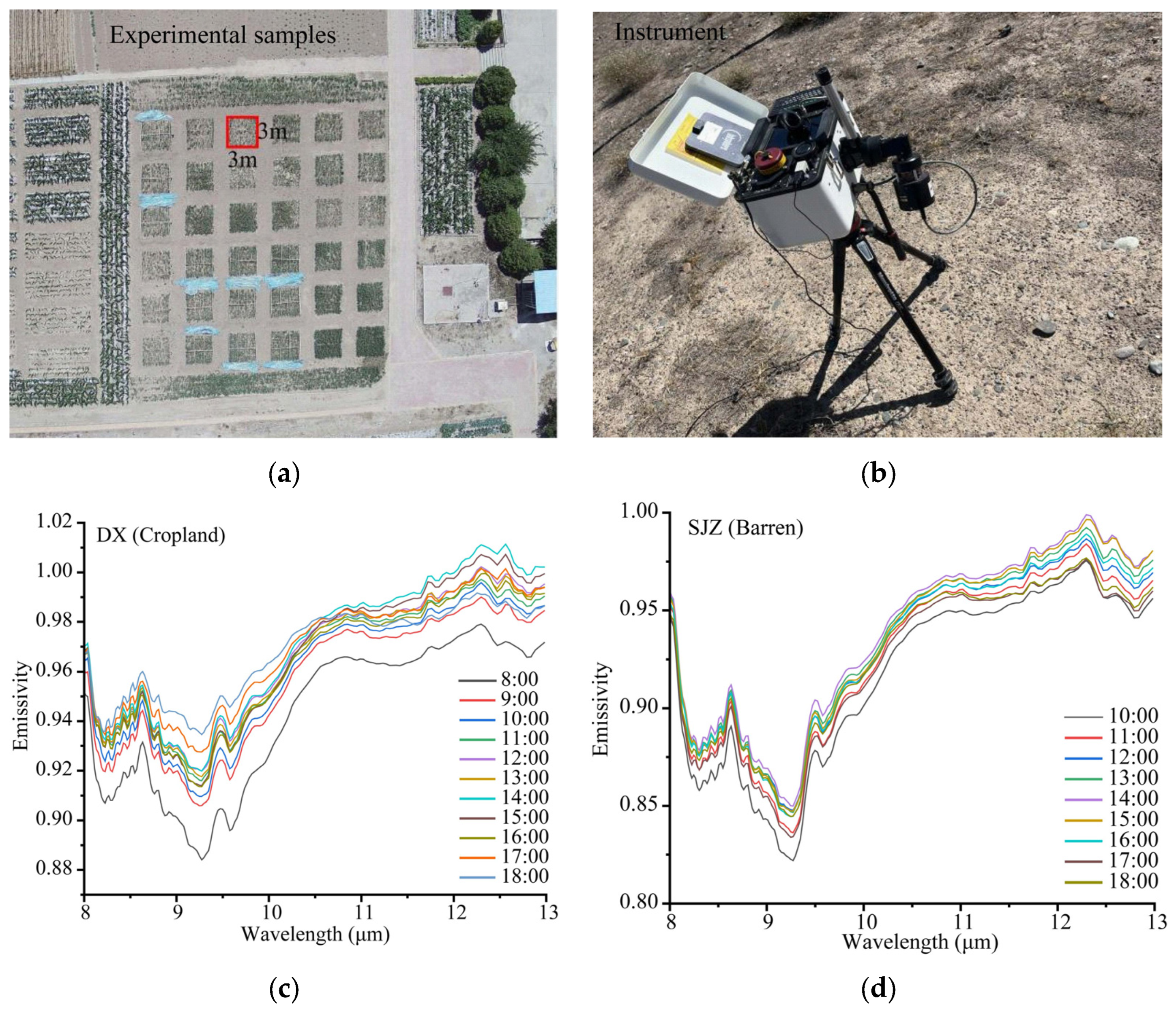
Experimental design for observing diurnal variation in LSE: Diurnal variation experiments were primarily conducted at the DX, XCD, SDB, YCZ, SJZ, and BLG stations, encompassing three predominant underlying surface types: barren, cropland, and grassland. Diurnal variation monitoring experiments were performed under clear-sky conditions, with measurements conducted at 30-min intervals from 08:00 to 18:00 Beijing time, as depicted in Figure 1. The LSE measurements were carried out in the following order: cold blackbody; warm blackbody; gold plate; sample. Finally, the sample emissivity curve was obtained by automatically setting Planck’s function (setting ε = 1.0 at 7–7.5 μm provides the initial temperature estimate essential for subsequent emissivity spectral retrieval). The calibrated aperture lens (field of view angle is 4.8°) was selected and the temperatures of warm and cold blackbody were set to 50 °C and 10 °C, respectively. Each scan was set to 8 times of spectral superposition, and it was always ensured that the Dewar bottle was filled with liquid nitrogen. Reflectance was primarily measured using a portable field spectroradiometer (ASD), where the reflectance spectrum of a target object is determined by comparing measurements against a standard whiteboard. Each target’s reflectance spectrum was finalized by averaging five consecutive measurements. Shallow soil moisture and temperature parameters were acquired through a WET sensor, which rapidly obtains data via probe insertion. The LST was captured using a FLIR high-end infrared thermal imager through photographic observation, with final LST values calculated by inputting the measured emissivity. Both the LST and shallow soil temperature/moisture data were obtained by averaging three repeated observational measurements.
(2)
Experimental design for observing vegetation effects on LSE: The experimental investigation into the influence of vegetation on LSE was implemented within the field trials at the DX station. A total of 30 experimental plots (3 m × 3 m) were established (Figure 1), wherein water regulation was applied to induce gradients in vegetation growth status and fractional cover. LSE and hyperspectral measurements were systematically acquired across these plots to characterize thermal infrared spectral curves under varying vegetation coverage conditions. Simultaneously, hyperspectral and thermal imaging data were synchronously acquired across the study area using unmanned aerial vehicles (UAVs). The observation requirements are shown in Table 1.
(3)
Experimental design for observing soil moisture effects on LSE: At the DX station, two adjacent 3 m × 3 m bare soil plots were established, one under natural rainfall conditions and the other subjected to manual irrigation to maintain consistently high soil moisture. The diurnal LSE variations were monitored in both plots to comparatively assess soil moisture impacts on emissivity. This configuration ensured identical soil properties and atmospheric conditions during the measurements, minimizing biases from soil texture variations and atmospheric disturbances. Furthermore, vegetation influence was deliberately excluded to isolate and prioritize the effects of soil moisture and temperature dynamics on the LSE.
(4)
Experimental design for observing LSE of different underlying surfaces: LSE measurements were executed across distinct land-use categories in northwestern China, including croplands (DX, PL, and SJZ-cropland), barren (SJZ-barren, YCZ, XCD, and SDB), and grasslands (BLG). These measurements, illustrated in Figure 2, facilitated a comparative analysis of LSE variations among differing soil types. The primary observation sites and their brief information are shown in Table 2.
The LSE and reflectivity values corresponding to each channel were calculated based on the spectral response function of the Fengyun-4A (FY-4A) satellite Advanced Geosynchronous Radiation Imager (AGRI) detector channels. The specific calculations are as follows [31]:
ε i = λ = m i n m a x [ β ( λ ) · ε λ ] / λ = m i n m a x β ( λ ) ,
where εi represents the LSE or reflectivity of the i-th channel, λ denotes the wavelength, min and max correspond to the minimum and maximum wavelengths of the spectral response function for the i-th channel, β(λ) is the spectral response percentage at wavelength λ, and ε(λ) is the LSE or reflectivity at wavelength λ measured on the ground.
(5)
LST data from continuous observation of relatively homogeneous sites: The observation data of LST primarily originated from the ARZ, HMZ, and DSL sites in 2020, provided by the National Tibetan Plateau Data Center (http://data.tpdc.ac.cn/zh-hans/, accessed on 14 February 2023). The geographical locations of these sites are illustrated in Figure 2. The underlying surfaces at the ARZ and DSL sites are relatively uniform grasslands, while the underlying surface at the HMZ site is a desert. The LST was observed using an infrared radiometer (model SI-III: instrument accuracy ±0.2 °C @ −10–65 °C; ± 0.5 °C @ −40–70 °C), with measurements conducted at 1 h. The observation sites and their brief information are shown in Table 2.
(6)
The soil component data were sourced from the China Soil Dataset provided by the National Tibetan Plateau Scientific Data Center. The nearest-neighbor interpolation method was employed to obtain the relevant soil component values for each observation site.

2.2. Methods

2.2.1. NDVI Threshold Method

The separation of LST and LSE remains a critical and persistent challenge in thermal infrared remote sensing retrieval. A widely adopted solution pathway involves first determining LSE using prior knowledge, followed by LST retrieval. Methods for retrieving ε and dε are primarily based on the Normalized Difference Vegetation Index (NDVI). These algorithms first utilize the NDVI to classify heterogeneous underlying surfaces and estimate the ε and dε across varying spatial scales through fractional vegetation cover. This approach is referred to as the NDVI threshold method. For example, Sobrino [32] proposed the following:
N D V I = ( r e f n i r r e f r e d ) / ( r e f n i r + r e f r e d ) ,
P v = ( N D V I N D V I m i n ) / ( N D V I m a x N D V I m i n ) ,
NDVI < 0.2,
ε = 0.98 0.42 r e f r e d ,
d ε = 0.003 0.029 r e f r e d ,
0.2 ≤ NDVI < 0.5,
ε 10.8 = 0.968 + 0.021 P v ,
ε 11.8 = 0.974 + 0.015 P v ,
ε = ( ε 10.8 + ε 11.8 ) / 2 ,
d ε = ε 10.8 ε 11.8 ,
NDVI ≥ 0.5,
ε = 0.989 ,
d ε = 0.0 ,
where refred and refnir represent the red and near-infrared band reflectance of the satellite detector. Pv denotes the vegetation cover fraction, calculated using NDVImax (under full vegetation conditions) and NDVImin (under bare soil conditions). The parameters retrieved using this method, such as LSE and LST, are labeled with the subscript “NDVI” for clarity.

2.2.2. Diurnal Variation Emissivity Model

The NDVI threshold method simplistically employs the NDVI to classify land surfaces for estimating the LSE parameters. However, in practice, LSE is closely linked to soil composition [14,15]. In this work, for scenarios where vegetation was excluded and only soil composition was considered, a new bare soil LSE parameter was estimated using the content of soil components: silt (USSL), sand (USS), organic matter (OMO), and clay (USCL), as follows:
ε s o i l = b 0 + b 1 U S S + b 2 U S S L + b 3 U S C L + b 4 O M O ,
Meanwhile, field experiments conducted by the authors and other researchers [19,22] have revealed that LSE is not only related to soil composition and vegetation but also closely linked to soil and atmospheric hydrothermal conditions. Notably, LSE exhibits distinct diurnal variation characteristics on daily time scales, as shown in Figure 3. To develop a new LSE inversion model that incorporates its own variation patterns, we adopted a “base state + perturbation” approach for modeling. The εsoil, determined by soil composition (Equation (12)), is defined as the base state, while the LSE variation caused by vegetation, land surface, and atmospheric hydrothermal conditions is treated as the perturbation.
Vegetation influences are exclusively constrained within the perturbation component. Integrating the LSE variation characteristics (as demonstrated in Figure 4), we developed an LSE inversion model specifically tailored for vegetated subsurface surfaces. Specifically, the soil LSE serves as the “base state”, while the vegetation status acts as a modulating factor, leading to a refined estimation model for LSE parameters:
ε n e w = c 0 N D V I + c 1 + ε s o i l ,
Parameters such as LSE and LST estimated using this method are labeled with the subscript “new”.
As a core radiative parameter characterizing land surface properties, LSE inherently exhibits strong coupling with LST [23]. When systematically accounting for diurnal-scale hydrothermal variations in both soil and atmospheric environments affecting LSE, while referencing radiative-LST covariation patterns [33] and incorporating diagnostic features from empirical LSE diurnal curves, as shown in Figure 3b, we posit that LSE’s daily variation conforms to a sinusoidal functional regime:
ε d a i l y ( t ) = ε s o i l + A s i n [ a 0 π ( t T r i s e ) / N t + B ] + a 1 ,
where parameters retrieved using this method (e.g., LSE and LST) are labeled with the subscript “daily”. Trise denotes the sunrise time, NT represents the daytime length, and t is the observation time. Reference [33] for Trise and NT estimation. As shown in Equation (14), “+a1” represents the “base state” of the underlying surface, while the term “Asin(a0π(t − Trise)/NT + B)” quantifies the perturbation caused by atmospheric, soil, and vegetation dynamics. Specifically, the factor’s influence on the perturbation component is predominantly encapsulated within parameters A and B. Consequently, for Equation (14), the critical task resides in establishing the computational methodology for determining these two parameters.

2.2.3. LST Inversion Algorithm

To compare the impacts of different LSE models on LST retrieval, this study implemented a split-window algorithm (Becker and Li, 1990) (B&L) [6] using FY-4A satellite data to evaluate the applicability of distinct LSE models.
Previous studies have demonstrated that the local split-window algorithm proposed by B&L exhibits favorable applicability in the arid and semi-arid regions of northwestern China [34]. However, this algorithm relies on prior knowledge of the LSE:
L S T = 1.274 + p ( B T 1 + B T 2 ) / 2 + m ( B T 1 B T 2 ) / 2 ,
p = 1.0 + 0.15616 ( 1 ε ) / ε 0.482 d ε / ε 2 ,
m = 6.26 + 3.98 ( 1 ε ) / ε + 38.33 d ε / ε 2 ,
where LST represents the retrieved land surface temperature in Kelvin (K), BT1 and BT2 denote the radiance brightness temperatures of two adjacent thermal infrared channels (typically centered at 10.8 μm and 11.8 μm, respectively), and p and m are parameters related to emissivity. ε and dε are the mean emissivity and emissivity difference of the two thermal infrared channels.
Implementation of the diurnal LSE variation model (Equation (14)) requires prior determination of parameters A and B. These parameters may vary significantly with different satellite remote sensing data sources. This study employed FY-4A/AGRI multispectral data as the foundational dataset.
By leveraging AGRI data to compute characteristic parameters representing land surface and atmospheric conditions, including channel reflectance, broadband albedo, vegetation indices, and thermal infrared radiance, synergistically integrated with diurnal LSE measurements (the measured sites are shown in Figure 2 as the “LSE observational sites”), we derived optimal computational models for parameters A and B through an enhanced Particle Swarm Optimization (PSO) algorithm [35], formulated as follows:
A = a 2 ( r e f n i r r e f r e d ) + a 3 a l b e d o + a 4 ,
B = a 5 ( L R 14 / L R 13 ) + a 6 a l b e d o + a 7 ,
Here, albedo denotes the top-of-atmosphere broadband albedo, formulated as follows [36]:
a l b e d o = 0.3376 r e f r e d 2 0.2707 r e f N I R 2 + 0.7074 r e f r e d r e f N I R + 0.2915 r e f r e d + 0.5256 r e f N I R
Equations (18) and (19) represent the currently optimal estimation models, statistically selected through systematic evaluation of diverse linear combinations of surface and atmospheric characteristic parameters using AGRI data, where LR13 and LR14 denote the thermal infrared radiance of the 13th and 14th channels of AGRI, which reflects the atmospheric water vapor status [37]. Coefficients a0−a7, b0−b4, c0−c1 in the LSE parameter estimation model were determined by averaging the results from 200 iterations of the PSO algorithm, based on the observational data. The total sample size for the ‘daily’ model using LSE data was 214, with 168 samples assigned to the training set and 46 reserved for validation. For the ‘new’ model utilizing LSE data, the total sample count was 109, comprising 63 training samples and 46 test samples. The εsoil model employed a total of 10 samples, all allocated for model training. Regarding LST impact assessment, the total dataset consisted of 5219 samples, all designated for model validation, as presented in Table 3. The primary workflow is shown in Figure 4.
Equation (13) quantifies vegetation influence on εnew and dεnew, where the positive coefficient c0 indicates a positive contribution of vegetation to both parameters. In Equation (12), the negative coefficient b1 denotes an inverse correlation between soil sand content and emissivity, while the positive coefficients b2–b4 signify positive correlations with clay, silt, and soil organic matter content, respectively. For the diurnal variation model: (refnir − refred) primarily characterizes vegetation status, albedo represents surface vegetation coverage and moisture conditions, and (LR14/LR13) indicates atmospheric water vapor status. Specifically: Amplitude A of ε increases with vegetation growth. Initial phase B of ε correlates negatively with atmospheric water vapor (LR14/LR13) and surface conditions (albedo). Amplitude A of dε decreases with vegetation growth but increases with surface moisture. Initial phase B of dε shows a positive correlation with atmospheric water vapor (LR14/LR13) and surface conditions (albedo). These mechanistic relationships align with the empirical patterns derived from field data analysis in Section 3.1.

3. Results

3.1. Diurnal Emissivity Variation Patterns and Dominant Influencing Factors Across Heterogeneous Surfaces

For bare soil underlying surfaces, to clarify the influence of soil composition on emissivity, measurements were conducted on bare soils across different underlying surfaces between 12:00 and 13:00 Beijing time (BJT). The emissivity spectra for these surfaces are shown in Figure 3a. Significant differences in emissivity among bare soils are observed within the 8–11 µm wavelength range, especially at 8–9.5 µm. This phenomenon is principally linked to the sand and moisture content variations in soils across different underlying surfaces. The measurements align with findings reported by Xiao et al. [14], demonstrating that soils with higher sand content exhibit lower emissivity at 8–9.5 µm. As visually corroborated in Figure 3a, this pattern manifests as progressively increasing emissivity values at 8–9.5 µm along the gradient from desert to farmland to grassland ecosystems. As shown in Figure 5a, the primary cause of emissivity variations across soil types in the 8–11 µm range stems from differences in sand, clay, and organic matter content. In contrast, within the 11–12 µm range, emissivity differences are predominantly driven by variations in clay content. Beyond 11 µm, emissivity exhibits greater uncertainty in its response to soil composition changes.
Figure 5b presents the correlation between the average emissivity (ε8_12) of 8–12 µm, the emissivity values (ε10.8 and ε11.8) of the 10.8 µm and 11.8 µm thermal infrared channels (the 12th and 13th channels of AGRI) used for LST retrieval, along with their mean (ε) and difference (dε) of ε10.8 and ε11.8, in relation to soil composition. The analysis reveals that ε8_12 exhibits significant positive correlations with soil organic matter (OMO) (p < 0.1) and clay content (USCL) (p < 0.05), contrasting with its significant negative correlation with sand content (USS) (p < 0.1). Notably, the 10.8 µm channel emissivity (ε10.8) demonstrates the strongest associations with soil constituents, showing significant positive associations with organic matter (p < 0.1), clay (p < 0.05), and silt content (USSL) (p < 0.1), while maintaining an inverse relationship with sand content (p < 0.05). In alignment with the spectral characteristics observed in Figure 3, the 11.8 µm channel emissivity (ε11.8) exhibits no statistically significant correlations with any soil components. This spectral band further displays minimal variation across soil types (<0.01 emissivity amplitude), confirming its insensitivity to pedological differentiation. The ε is predominantly influenced by silt and sand content dynamics, whereas the dε primarily responds to variations in organic matter, clay, and sand content.
The LSE of bare soil exhibits dual dependencies, being influenced not only by soil composition but also by surface hydrothermal conditions. Figure 6 demonstrates temporal variations (excluding winter) in ε8_12 and associated parameters for identical bare soil surfaces. The LSE anomalies predominantly show inverse phase relationships with shallow soil moisture anomalies (0–10 cm depth), indicating LSE suppression under increasing moisture content. Conversely, these LSE anomalies maintain phase coherence with both shallow soil temperature and thermal infrared temperature anomalies, revealing LSE enhancement during thermal elevation events.
Utilizing observations under identical bare soil substrates, this approach eliminates LST variations induced by soil composition, focusing exclusively on the hydrothermal effects on the LSE. An existing study [23] has demonstrated a strong coupling effect between LSE and LST, indicating that LSE increases with rising LST. Consistently, our observations reveal a statistically significant positive correlation between LSE and LST (Figure 6c,d), corroborating established research conclusions. Xiao et al. [14] demonstrated through laboratory measurements of soil samples with varying moisture contents (excluding temperature effects) that LSE at 8–9.5 µm positively correlates with soil moisture prior to saturation. However, the magnitude of moisture’s influence on LSE varies with soil composition and state. Crucially, under controlled laboratory conditions, soil moisture solely functions as a compositional factor of soil affecting LSE. In natural settings, moisture concurrently modulates thermal dynamics: soils with higher moisture content exhibit reduced LST fluctuations. This dual mechanism enables soil moisture to suppress LST elevation, thereby decelerating LSE increase and ultimately manifesting a significant negative LSE and moisture correlation (R = −0.86, p < 0.01) as evidenced in Figure 6b. The fundamental discrepancy between laboratory measurements and field observations constitutes a critical research frontier requiring prioritized investigation.
LSE over vegetated terrain demonstrates coupled dependence on vegetation coverage density and phenological status. Figure 7 delineates emissivity divergence across maize phenophases, revealing significant spectral modifications driven by crop ontogeny. Physiologically active maize stands exhibit a well-defined absorption trough centered at 9.6 µm, which undergoes progressive attenuation through maturation stages due to foliar water loss, culminating in complete feature extinction during senescence. This is consistent with previous studies [38] indicating that leaf moisture is the main cause of changes in green vegetation emissivity. The statistical modeling in Figure 7c establishes robust covariance between 9.6 µm emissivity (ε9.6) and canopy leaf area index (LAI) (R = 0.69, p < 0.01). The analysis demonstrates that senesced crop canopies develop a prominent 9.1 µm absorption trough and characteristic dual-trough morphology spanning 10.0–12.5 µm. The integration of these state-dependent emissivity signatures enables dynamic monitoring of vegetation vigor and precision assessment of agricultural disasters.
By leveraging the AGRI detector channel specifications and spectral response functions, we systematically derived channel-specific reflectance and emissivity spectra by Equation (1) to investigate vegetation–emissivity coupling in LST retrievals. Figure 8 reveals significant correlation between thermal infrared (TIR) channel emissivity metrics (mean, difference, ratio) and the NDVI. The mean channel emissivity (ε = (ε10.8 + ε11.8)/2) and ratio (ε10.811.8) exhibit significant positive correlations with the NDVI (R > 0.75, p < 0.01), and emissivity difference (dε = ε10.8 − ε11.8) shows inverse correlation (R = −0.84, p < 0.01). These systematic relationships confirm vegetation dynamics as the primary modulator of emissivity variations in vegetated terrain. In the retrieval of LST, incorporating the constraint relationship between the LSE and NDVI to replace assumptions about variations in LSE itself is expected to enhance the accuracy of land surface temperature retrieval.
Synthesizing these findings, LSE exhibits dual modulation from both intrinsic soil composition and dynamic hydrothermal–vegetation interactions. For non-vegetated croplands, annual LSE variations driven by soil-atmosphere hydrothermal dynamics demonstrate limited magnitude (Δε = 0.05), whereas surface transitions from bare soil to full vegetation coverage induce substantially greater LSE divergence (Δε = 0.07) as quantitatively resolved in Figure 5b.

3.2. Diurnal-Scale Characteristics of Emissivity Variations and Their Dominant Drivers

The diurnal emissivity dynamics of natural surfaces exhibit significant departure from laboratory-controlled conditions, governed by solar radiative forcing and coupled soil–vegetation–atmosphere interactions. Figure 9 delineates the time-resolved spectral emissivity (8–14 µm) of bare agricultural soil, revealing three principal observational constraints: (1) spectral stability: wavelength-dependent consistency with enhanced noise post−12 µm, justifying LSE averaging among 8–12 µm (ε8_12); (2) diurnal hysteresis: diurnal hysteresis with maximum ε8_12 at solar noon and minima during twilight (Δε = 0.025) as shown in Figure 9; (3) channel-specific responses: the 10.8 and 11.8 µm mean LSE (ε) demonstrate systematic positive bias (≈0.015 vs. ε8_12) following inverted-U patterns, while their differential LSE (dε) exhibits U-shaped diurnal variability.
Field measurements under the same atmospheric conditions reveal fundamental soil emissivity thermodynamics. The figure (figure omitted) is similar to Figure 6. The LSE differential between rain-fed and permanently irrigated plots (εdry − εwet) demonstrates a positive correlation with the shallow soil thermal dynamics, a negative correlation with the surface moisture content, and tight coupling with the LST. The dynamic interdependence between LSE and LST drives a critical thermodynamic regulation: aqueous-phase dynamics in moist soils attenuate diurnal LST escalation through latent heat flux dominance, thereby enacting a suppressive effect on LSE enhancement that manifests as a significant negative correlation between spectral LSE and soil moisture content.
Contemporary land surface process models exhibit critical LSE parameterization deficiencies by neglecting thermohydrological co-regulation mechanisms, instead implementing static categorical constants that fail to replicate observed diurnal LSE fluctuations. This study establishes a data-driven diurnally varying parameterization framework, thereby enhancing LST retrieval accuracy and longwave radiation estimation precision through phase-synchronized energy.
For vegetated surfaces, due to incomplete vegetation coverage across vegetated underlying surfaces, the soil hydrothermal conditions remain capable of influencing the LSE. Consequently, LSE measurements over vegetated surfaces exhibit detectable diurnal variability, albeit with reduced magnitudes compared to bare soil underlying surfaces, as demonstrated in Figure 5b. When comparing diurnal variation characteristics across underlying surfaces (Figure 1 and Figure 3b), desert surfaces exhibit greater diurnal emissivity variations than bare cropland soils under equivalent moisture conditions, while bare cropland soils show larger diurnal emissivity fluctuations than vegetated surfaces. Analysis of emissivity measurements across different time periods reveals that emissivity stabilizes or exhibits minimal variation once the surface is fully heated. Therefore, we recommend conducting emissivity measurements for diverse underlying surfaces during this stabilized period (12:00–16:00 BJT).

3.3. Quantifying Emissivity-Induced Uncertainties in Diurnal Land Surface Temperature Retrievals

To evaluate LST retrieval sensitivity to LSE, Figure 10 presents ΔLST variations with ε and dε using clear-sky data from the ARZ station (January–October 2020). ΔLST induced by ε and dε variations consistently correlates with the sum (BT12 + BT13)/difference (BT12 − BT13) of thermal infrared brightness temperatures and with the reflectance difference between near-infrared and red bands (ref3 − ref2). A 0.1 change in ε or dε causes ΔLST < 2.0 K. When ε increases from 0.90 to 1.00, the LST decreases by 3.0–7.0 K. With dε increasing from −0.05 to 0.05, the LST decreases by 10–18 K. These results demonstrate that LSE significantly impacts LST retrieval accuracy, confirming that precise emissivity estimation is crucial for improving LST retrieval precision.
The model was rigorously validated using diurnal LSE measurements coupled with LST data from three relatively homogeneous sites (the HMZ, ARZ, and DSL sites). As depicted in Figure 11 and Figure 12, the retrievals demonstrate significant concordance (R > 0.7; p < 0.01) between estimated and observed values for broadband LSE ε8_12, channel-specific means ε, and LSE difference dε. Notably, the NDVI threshold method exhibits paradoxical behavior with strong inverse correlation in ε (R = −0.88, p < 0.01; RMSE = 0.016). Implementation of the LSE parameters within the local split-window algorithm, as shown in Figure 12a, derived diurnal LST variations that exhibited strong concordance with in situ measurements (R = 0.98, p < 0.01) yet were characterized by substantial deviations (RMSE = 6.02 °C). A persistent overestimation bias (+10 °C mean offset) dominated sub-ambient thermal regimes (LST < 20 °C), contrasting with progressive underestimation trends (−4.0 °C mean offset) under hyperthermal conditions (LST > 45 °C), collectively revealing thermally stratified error propagation in the retrieval framework.
Figure 11c,d present comparative analyses of ε derived from the empirically modified NDVI threshold method against ground measured values. Post-calibration, retrievals at 10.8 µm and 11.8 µm spectral bands exhibit a statistically significant positive correlation with in situ data (R = 0.83, p < 0.01), achieving a reduced RMSE of 0.008. Conversely, dε estimates display an inverse relationship with field measurements (R = −0.72, p < 0.01), albeit with further error contraction to an RMSE of 0.005. The refined LSE framework demonstrates enhanced performance in geostationary satellite-based LST retrievals, as evidenced in Figure 12b, where the RMSE decreases to 4.94 °C, which is relatively smaller compared to the operational Fengyun (FY) satellite LST product (RMSE = 5.94 °C). Notably, errors in low-temperature regimes (LST < 20 °C) are mitigated through LSE model optimization.
Figure 11e,f show the validation of the newly developed diurnal LSE model against ground in situ measurements, with modeled ε and dε values demonstrating robust agreement (R = 0.87, p < 0.01, RMSE = 0.007; R = 0.85, p < 0.01, RMSE = 0.004, respectively). The model accurately resolves diurnal LSE variability, capturing amplitude fluctuations in LSE. Implementation of this temporally resolved LSE framework elevates LST retrieval precision to an RMSE of 3.35 °C—a 2.70 °C reduction relative to the original NDVI threshold method, as evidenced in Figure 12c. Notably, errors in low and high temperature regimes (LST < 20 °C and LST > 45 °C) are mitigated through the newly developed diurnal LSE model.
Figure 11g,h present comparative validation of 8–12 µm broadband LSE ε8_12 retrievals by the enhanced NDVI threshold method and the new diurnal variation model. The revised NDVI approach demonstrates an LSE RMSE of 0.012, inducing reduced LST retrieval errors (RMSE = 3.80 °C) at three observational sites (Figure 13a) compared to ε implementation. Conversely, the diurnal variation model achieves superior ε8_12 precision (RMSE = 0.007), with systematic bias comparable to channel-specific emissivity retrievals, though with a systematic 0.015 underestimation relative to two thermal infrared channels’ mean values. Implementation of this diurnal LSE framework in geostationary satellite processing reduces LST retrieval errors to 2.97 °C RMSE (Figure 13b), a 3.00 °C improvement over the NDVI baseline. This advancement primarily addresses the LSE diurnal change in bare soil regions, while maintaining sub−3.0 °C accuracy of the LST across all terrains, as shown in Figure 14.
As shown in Figure 3a, the LSE of different bare soils displays significant variations within the 8–12 µm range, with particularly pronounced differences observed between 8 and 9.5 µm. This is primarily attributed to the sensitivity of the 8–9.5 µm spectral band to soil components such as sand and moisture content [14]. Considering that thermal infrared spectra lose sensitivity to soil types beyond 12 µm, the ε8_12 more effectively reflects the differences in underlying surface composition. By integrating ε8_12 into retrieval algorithms, the method inherently accommodates soil-specific spectral signatures, reducing mineralogy-induced LST biases by 0.4–1.1 °C compared to narrowband approaches. This broadband strategy achieves superior agreement with in situ LST measurements (R = 0.99, p < 0.001, RMSE = 2.97 °C), by operationally decoupling soil-type dependencies from thermal radiation physics without compromising diurnal LSE trends. As shown in Figure 15, compared across different underlying surface types, the LST estimated using the diurnal LSE variation model based on ε8–12 demonstrates improved accuracy over the NDVI threshold method for all land surface types. This enhancement is particularly pronounced over grasslands, where the RMSE of the LST retrieved by the NDVI threshold method decreased significantly from 8.14 °C to 3.17 °C after applying the diurnal variation model.
A comparative evaluation of the NDVI threshold method and the diurnal variation inversion model reveals distinct performance characteristics. The NDVI threshold approach generates LSE estimates with attenuated diurnal variability (Δε < 0.01), effectively collapsing the temporal dynamics toward daily median values. This intrinsic amplitude suppression manifests as statistically ambiguous correlations with ground observations, particularly evident in the anomalous inverse relationship displayed in Figure 11d (R = −0.72, p < 0.01). Conversely, the physics-constrained diurnal variation model resolves full-spectrum LSE trajectories that preserve phase-synchronized variations with in situ measurements. As demonstrated in Figure 11e,f, the model-derived estimates exhibit evenly distributed scatter across the LSE variation domain (RMSE < 0.008), maintaining a robust positive correlation (R > 0.8, p < 0.01) that reflects stable physical consistency between retrieved and observed thermal properties.

4. Discussion

The hyperspectral NDVI was computed using UAV-acquired data (14:00 Beijing time, 22 June 2024) over the desert underlying surface of Shajing Town, incorporating red and near-infrared band reflectance under AGRI channel response functions. The mean channel emissivity (ε) and 8–12 μm broadband emissivity (ε8_12) were subsequently derived through Equations (18) and (19), respectively, as demonstrated in Figure 16. The emissivity estimated via the NDVI threshold method was primarily concentrated around 0.97, while that estimated by the diurnal variation model ranged between 0.93 and 0.96. The ε retrieved by the NDVI threshold method (εNDVI) was consistently lower than the ε8_12 derived from the diurnal variation model (εdaily). Although the spatial distributions of the retrieved LST based on εNDV and εdaily exhibited similarities, the LST values inverted using εdaily were generally higher than those based on εNDVI.
Figure 17 presents temporal variations in the LSE parameters and LST frequency distributions across the study area. The diurnal variation model revealed a progressive shift in the εdaily emissivity peak from 0.947 at 12:00 BJT to 0.942 by 17:00 BJT, indicative of thermal emissivity attenuation with increasing solar exposure. Conversely, εNDVI demonstrated exceptional temporal stability, maintaining values near 0.97 throughout the observation periods with Δε < 0.001. The corresponding LST distributions initially showed convergence between algorithms at 12:00 BJT (predominantly 22 °C) under lower thermal loading conditions. Divergence emerged progressively with intensified surface heating, reaching notable disparities by 14:00 BJT when εdaily-based LST estimates clustered in the 41–44 °C range, systematically exceeding εNDVI-derived values by 0.7 °C. These UAV observations corroborated the findings from Section 3.3, demonstrating the diurnal variation model’s capacity to rectify the characteristic underestimation (particularly LST > 45 °C) inherent in the B&L algorithm, thereby achieving enhanced LST retrieval fidelity through changing LSE compensation.
When soil component data were unavailable, preliminary implementations of the diurnal variation inversion model employing ε8_12 parameters yielded LST retrievals through the B&L algorithm as illustrated in Figure 18. Comparative evaluation against Figure 13b demonstrated a 0.8 K reduction in RMSE for LST estimates following soil component integration, confirming the substantial influence of soil composition on LSE modulation. The influence of soil composition on LSE is primarily governed by the radiative properties of soil constituents such as sand fractions, organic matter, and clay content. Variations in the proportional abundance of these components form distinct soil types, inducing alterations in bulk soil radiative characteristics that lead to statistically significant differences in LSE.
This study characterized LSE variations across crop conditions (Figure 7), revealing the sensitivity of emissivity at the 9.1 µm, 9.6 µm, and 11.5 µm bands to vegetation status. These signatures enable vegetation monitoring and yield estimation in practice. Additionally, LSE correlations with soil moisture/temperature (Figure 6) offer new approaches for land surface model parameterization: (1) rapid soil emissivity calculation using soil composition inputs; (2) dynamic LSE parameterization schemes based on observed relationships (Figure 6), enhancing model interpretability and accuracy. Furthermore, LSE characterization directly improves LST retrieval: (1) replacing static emissivity models with dynamic variants in prior-knowledge algorithms; (2) applying sensitivity constraints (e.g., inverse NDVI–emissivity difference relationship in Figure 8) and boundary conditions (e.g., diurnal LSE variation magnitudes across surfaces in Figure 3) to boost joint LSE/LST inversion precision.
However, the model has certain limitations, primarily manifested in three aspects. (1) The model uses reflectance as an input parameter (Equations (18)–(20)). However, this becomes inapplicable during nighttime due to missing visible-channel reflectance values. Additionally, at sunrise and sunset, satellite visible-channel reflectance proves less effective for vegetation characterization owing to enhanced atmospheric scattering and low solar elevation angles, potentially leading to larger model errors. (2) Soil composition data derive from existing datasets (China Soil Dataset provided by the National Tibetan Plateau Scientific Data Center), without co-located soil sample analysis for LSE validation, causing model errors. (3) There are insufficient training samples for soil emissivity modeling. Current observations mainly represent bare soils in Northwest China (loess, sandy, Gobi, and desert types), lacking data from contrasting soils like Northeast chernozem and Southwest purple/latosol soils. Future expansion of bare-soil emissivity observations will enhance model applicability and estimation accuracy. (4) Similar to the regional limitations in soil emissivity modeling, the observed diurnal LSE variations and hydrothermal responses are exclusively from Northwest China. Additional diurnal LSE monitoring across diverse soils and environmental conditions is needed to improve model generalizability.
Inspired by field measurements and prior research, this study established a land surface condition-driven LSE model and characterized LSE variations. However, this work remains preliminary, having multiple shortcomings. We will continuously improve model precision and applicability through expanded datasets and analytical methods. We also aim to disseminate the dynamic LSE modeling concept, encouraging broader research efforts to advance land surface parameterization and LST retrieval.

5. Conclusions

Building on multi-seasonal field campaigns incorporating hyperspectral observations, this study employed signal decomposition techniques to characterize LSE change regulation across heterogeneous land surfaces. Through synergistic analysis of ground-truth datasets, we systematically came to the following conclusions:
(1)
Thermal emissivity signatures demonstrate marked spectral stratification across surface cover classes. Bare soil substrates exhibit substantial emissivity disparities (8–11 µm), particularly in the dual absorption troughs spanning 8–9.5 µm where emissivity variations show composition-dependent patterns: strongly anti-correlated with sand fraction (R = −0.68, p < 0.1) versus positive correlations with clay (R = 0.77, p < 0.05) and organic content (R = 0.65, p < 0.1) across the 8–12 µm spectrum. Vegetation canopies present a diagnostic absorption trough at 9.6 µm, whereas senescent plant residues develop distinct spectral fingerprints featuring a primary trough at 9.1 µm accompanied by secondary absorption features through 10–12.5 µm. Post-senescence transformation processes, as observed in wheat stubble, progressively attenuate these spectral features in the 8–12 µm range, generating statistically significant emissivity contrasts relative to both bare soils and photo-synthetically active vegetation. These wavelength-specific emissivity differentials facilitate operational monitoring frameworks through land cover classification using absorption trough depth indices and crop phenology tracking via temporal emissivity trajectory analysis in thermal infrared bands.
(2)
Emissivity drivers exhibit fundamental divergences across land cover types. Beyond the universal regulation by soil mineralogy, bare surfaces demonstrate a pronounced anti-correlation with shallow soil moisture (R = −0.86, p < 0.01) and a strong thermal coupling with surface thermal regimes, whereas vegetated terrains manifest hybrid radiative contributions from both soil and canopy elements. Vegetation emissivity dynamics operate through dual-path modulation: while being partially constrained by subsurface hydrothermal conditions, they show tighter covariation with vegetation density and phenological status as quantified by seasonal leaf area index trajectories.
(3)
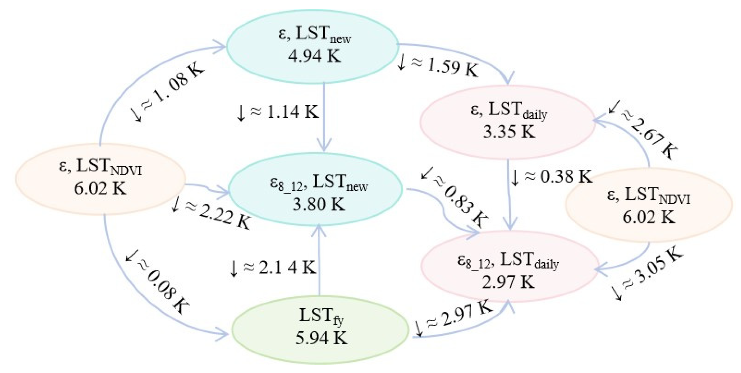
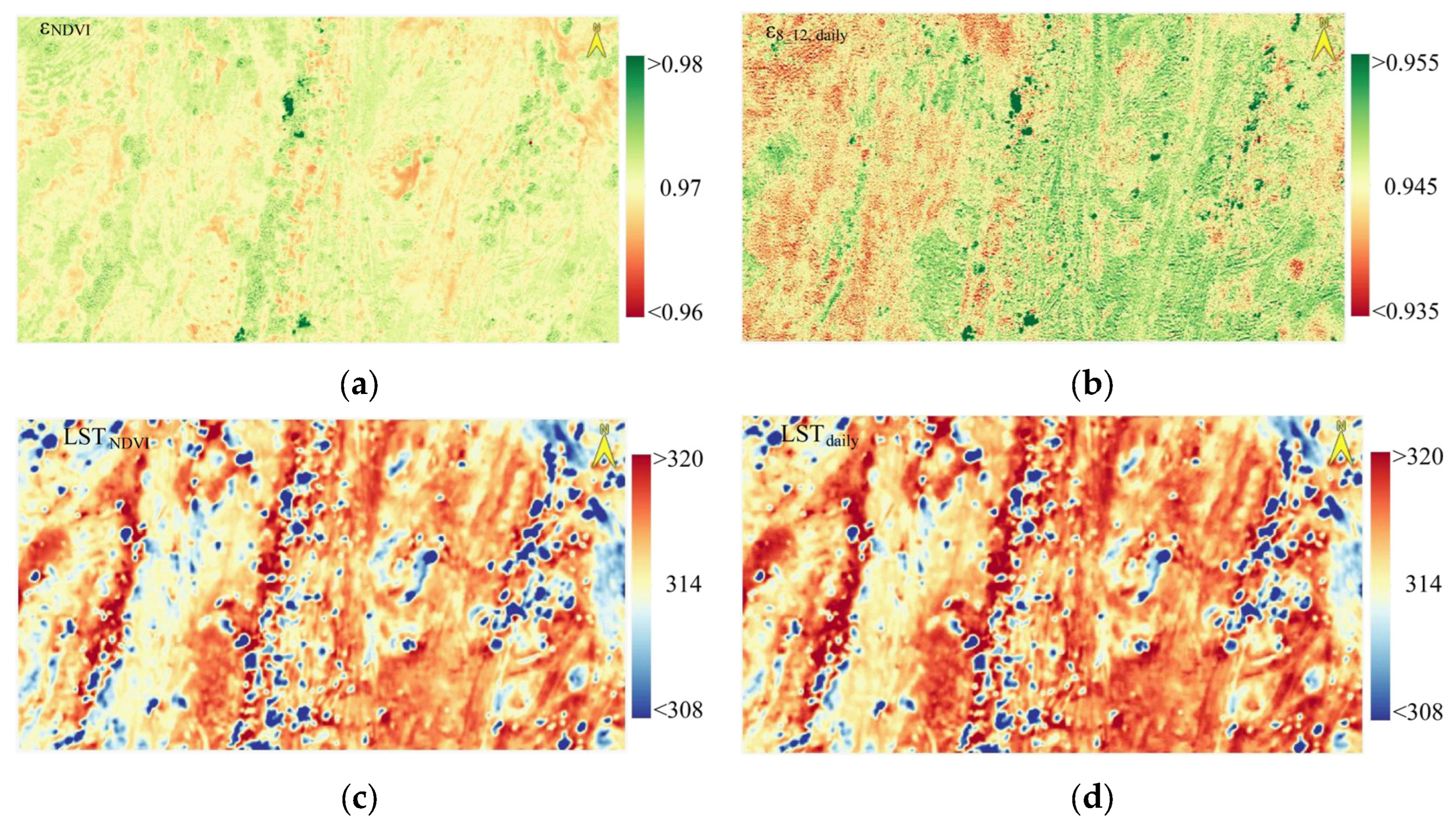
Incorporating emissivity diurnal dynamics substantially improves LST retrieval precision. On daily cycles, emissivity variations (Δε ≈ 0.025 amplitude) primarily stem from soil hydrothermal modulation, exhibiting phase coupling with insolation-driven thermal inertia transitions. Our retrieval framework establishes a baseline emissivity through soil constituent unmixing, with perturbation terms quantifying soil moisture–thermal gradient interactions, atmospheric path radiance effects, and vegetation-mediated emissivity depression. Spectral optimization reveals 8–12 µm broadband emissivity optimally captures substrate physical heterogeneity. Implementing this diurnal variation model in geostationary satellite processing reduces LST retrieval errors from 6.02 °C (conventional split-window algorithm) to 2.97 °C RMSE, achieving < 3.0 °C accuracy through considering the diurnal variation characteristics of emissivity.

Author Contributions

Conceptualization, L.W. and S.S.; methodology, P.Y. and D.H.; validation, Y.Y., X.J. and X.R.; resources, L.W. and X.W.; writing—original draft preparation, L.W.; writing—review and editing, L.W., H.H. and P.Y. All authors have read and agreed to the published version of the manuscript.

Funding

This research was funded by the National Natural Science Foundation Joint Fund Project (Grant number U2142208), the Natural Science Foundation of Gansu Province Project (Grant number 24JRRA723), Gansu Provincial Science and Technology Plan Project (Joint Research Fund—General Program) (25JRRA1110), the National Natural Science Foundation of China (Youth Found) (Grant number 42105131), the Fengyun-3 Meteorological Satellite Ground Application System Engineering Project (Grant number FY-3(03)-AS-12.11-ZT), and the Public Relations/Co-creation Fund Project of the Institute of Arid Meteorology, the CMA (Grant number JYGG202307).

Data Availability Statement

The data of FY-4 can be download from the website http://satellite.nsmc.org.cn/DataPortal/cn/home/index.html (accessed on 30 October 2024), and the ground in situ data will be made available on request.

Conflicts of Interest

The authors declare no conflicts of interest.

References

  1. Li, Z.; Wu, H.; Duan, S.; Zhao, W.; Ren, H.; Liu, X.; Pei, L.; Tang, R.; Ye, X.; Zhu, J.; et al. Satellite remote sensing of global land surface temperature: Definition, methods, products, and applications. Rev. Geophys. 2023, 61, e2022RG000777. [Google Scholar]
  2. Becker, F. The Impact of Spectral Emissivity on the Measurement of Land Surface Temperature from a Satellite. Int. J. Remote Sens. 1987, 8, 1509–1522. [Google Scholar] [CrossRef]
  3. Zheng, X.; Li, Z.; Nerry, F.; Zhang, X. A New Thermal Infrared Channel Configuration for Accurate Land Surface Temperature Retrieval from Satellite Data. Remote Sens. Environ. 2019, 231, 111216. [Google Scholar] [CrossRef]
  4. Cheng, J.; Liu, Q.; Li, X.; Xiao, Q.; Liu, Q.; Du, Y. The Correlation Based Thermal Infrared Temperature and Emissivity Separation Algorithm. Sci. Sin. Terrae 2008, 38, 261–272. [Google Scholar]
  5. Wan, Z.; Li, Z. A Physics-Based Algorithm for Ret Retrieving Land—Surface Emissivity and Temperature from EOS/MODIS Data. IEEE Trans. Geosci. Remote Sens. 1997, 35, 980–996. [Google Scholar]
  6. Becker, F.; Li, Z. Towards a Local Split-Window Method over Land Surfaces. Int. J. Remote Sens. 1990, 11, 369–393. [Google Scholar]
  7. Kahle, A.B.; Madura, D.P.; Soha, J.M. Middle Infrared Multispectral Aircraft Scanner Data: Analysis for Geologic Applications. Appl. Opt. 1980, 19, 2279–2290. [Google Scholar]
  8. Watson, K. Two-Temperature Method for Measuring Emissivity. Remote Sens. Environ. 1992, 42, 117–121. [Google Scholar]
  9. Watson, K. Spectral Ratio Method for Measuring Emissivity. Remote Sens. Environ. 1992, 42, 113–116. [Google Scholar]
  10. Labed, J.; Stoll, M.P. Angular Variation of Land Surface Spectral Emissivity in the Thermal Infrared: Laboratory Investigations on Bare Soils. Int. J. Remote Sens. 1991, 12, 2299–2310. [Google Scholar]
  11. Tang, B.; Li, Z. Evaluation of an ASTER Emissivity Product with Field Spectral Radiance Measurements for Natural Surfaces. Int. J. Remote Sens. 2019, 40, 1709–1723. [Google Scholar]
  12. Li, X.; Liu, S.; Xiao, Q.; Ma, M.; Jin, R.; Che, T.; Wang, W.; Hu, X.; Xu, X.; Wen, J. A Multiscale Dataset for Understanding Complex Eco-Hydrological Processes in a Heterogeneous Oasis System. Sci. Data 2017, 4, 170083. [Google Scholar] [CrossRef] [PubMed]
  13. Zhang, Y.; Ni, L.; Hua, W.; Jiang, X.; Ying, H. Fast and Accurate Measurement of Spectral Emissivity with a Portable Field Infrared Spectrometer: Ancillary Equipment and Methods. Int. J. Remote Sens. 2019, 40, 1736–1749. [Google Scholar]
  14. Xiao, Q.; Liu, Q.; Li, X.; Chen, F.; Xin, X. A Field Measurement Method of Spectral Emissivity and Research on the Feature of Soil Thermal Infrared Emissivity. J. Infrared Millim. Waves 2003, 22, 373–378. [Google Scholar]
  15. Cheng, J.; Xiao, Q.; Li, X.; Liu, Q.; Du, Y. Algorithm Research of Soil Emissivity Extraction. Natl. Remote Sens. Bull. 2008, 12, 699–706. [Google Scholar]
  16. Hu, J.; Tang, S.; Dong, L.; Zhang, Y. Analysis of Thermal Infrared Emissivity for Sand Dust Source Regions in Northwest China. J. Infrared Millim. Waves 2013, 32, 550–554. [Google Scholar]
  17. Liu, Y.; Ali, M.; Huo, W.; Yang, X.; Liu, X.; He, Q. Characteristics of Land Surface Emissivity on Distribution and Variation in Taklimakan Desert. Desert Oasis Meteorol. 2014, 8, 1–7. [Google Scholar]
  18. Huang, Q.; Shi, Z.; Pan, G.; Ji, W. Characteristics of Thermal infrared Hyperspectral and Prediction of Sand Content of Sandy Soil. Spectrosc. Spectr. Anal. 2011, 31, 2195–2199. [Google Scholar]
  19. Wang, L.; Guo, N.; Zuo, H.; Wang, W. Optimization of the Local Split-Window Algorithm for FY-4A Land Surface Temperature Retrieval. Remote Sens. 2019, 11, 2016. [Google Scholar] [CrossRef]
  20. Xia, J.; Zhang, F. A Study on Remote Sensing Inversion of Soil Salt Content in Arid Area Based on Thermal Infrared Spectrum. Spectrosc. Spectr. Anal. 2019, 39, 1063–1069. [Google Scholar]
  21. Zhuge, X.; Zou, X.; Weng, F.; Sun, M. Dependence of Simulation Biases at AHI Surface-Sensitive Channels on Land Surface Emissivity over China. J. Atmos. Ocean. Technol. 2018, 35, 1283–1298. [Google Scholar]
  22. Zheng, Z.; Wei, Z.; Li, Z.; Chen, C. A Study of Variation Characteristics of Surface Broadband Emissivity over Three Typical Bare Soil Underlying Surfaces in Northwestern China. Chin. J. Atmos. Sci. 2016, 40, 1227–1241. (In Chinese) [Google Scholar]
  23. Tang, L.; Chen, X.; Wang, J.; Zhao, H.; Huang, Q. A Study of the Coupling Relationship Between Concrete Surface Temperature and Concrete Surface Emissivity in Natural Conditions. Spectrosc. Spectr. Anal. 2014, 34, 1736–1741. [Google Scholar]
  24. Zhao, S.; Hu, X.; Jing, X.; Jiang, S.; He, L.; Ma, A.; Yang, L. Analyses of Land Surface Emissivity Characteristics in Mid-Infrared Bands. Spectrosc. Spectr. Anal. 2018, 38, 71–77. [Google Scholar]
  25. Wang, H. Extraction of Emissivity Information from Thermal Infrared Remote Sensing and Modeling of Soil Emissivity; University of Chinese Academy of Sciences: Beijing, China, 2014. [Google Scholar]
  26. Wang, H.; Pan, Y.; Li, H.; Yao, M. Measuring Spectral Emissivity of Natural Objects with FTIR. Infrared Technol. 2009, 31, 210–214. [Google Scholar]
  27. Masiello, G.; Serio, C.; Venafra, S.; Liuzzi, G.; Gottsche, F.; Trigo, I.; Watts, P. Kalman Filter Physical Retrieval of Surface Emissivity and Temperature from SEVIRI Infrared Channels: A Validation and Inter Comparison Study. Atmos. Meas. Tech. 2015, 8, 2981–2997. [Google Scholar]
  28. Wang, H.; Mao, K.; Yuan, Z.; Shi, J.; Cao, M.; Qin, Z.; Duan, S.; Tang, B. A method Forland Surface Temperature Retrieval Based on Model-Data-Knowledge-Driven and Deep Learning. Remote Sens. Environ. 2021, 265, 112665. [Google Scholar] [CrossRef]
  29. Zheng, X.; Guo, Y.; Zhou, Z.; Wang, T. Improvements in Land Surface Temperature and Emissivity Retrieval from Landsat-9 Thermal Infrared Sata. Remote Sens. Environ. 2024, 315, 114471. [Google Scholar] [CrossRef]
  30. Dai, W.; Mao, K.; Guo, Z.; Qin, Z.; Shi, J.; Bateni, S.M.; Xiao, L. Joint Optimization of AI large and Small Models for Surface Temperature and Emissivity Retrieval Using Knowledge Distillation. Artif. Intell. Agric. 2025, 15, 407–425. [Google Scholar]
  31. Shen, H.; Shen, H. Effect of Relative Spectral Response and Bandwidth on Water-Leaving Reflectance of Optically Complex Case II Waters. Infrar 2012, 33, 31–37. [Google Scholar] [CrossRef]
  32. Sobrino, J.A.; Raissouni, N.; Li, Z. A Comparative Study of Land Surface Emissivity Retrieval from NOAA Data. Remote Sens. Environ. 2001, 75, 256–266. [Google Scholar] [CrossRef]
  33. Xie, X. Estimation of Daily Evapo-transpiration (ET) from One Time-of -Day Remotely Sensed Canopy Temperature. Remote Sens. Environ. China 1991, 6, 254–260. [Google Scholar]
  34. Wang, L.; Zuo, H.; Chen, J.; Dong, L.; Zhao, J. Land Surface Temperature and Sensible Heat Flux Estimated from Remote Sensing over Oasis and Desert. Plateau Meteorol. 2012, 31, 646–656. [Google Scholar]
  35. Kenny, J.; Eberhart, R. Particle Swarm Optimization. In Proceedings of the IEEE International Conference on Neural Networks, Athens, Greece, 16–21 July 2006; IEEE: Piscataway, NJ, USA, 2006; Volume 4, pp. 1942–1948. [Google Scholar]
  36. Song, L.; Gao, W. An Improved Method to Derive Surface Albedo from Narrowband AVHRR Satellite data: Narrowband to Broadband version. J. Appl. Meteorol. 1999, 38, 239–249. [Google Scholar]
  37. Wang, L.; Zuo, H.; Wang, W. A Simple Method for Surface Radiation Estimating Using FY-4A Data. J. Appl. Meteorol. Climatol. 2021, 60, 763–777. [Google Scholar] [CrossRef]
  38. Yang, L. Study on Near Infrared Reflectance Spectroscopy and Emissivity of Green Vegetation Simulated by LDHs; Nanjing University of Aeronautics and Astronautics: Nanjing, China, 2025. [Google Scholar]
Figure 1. Experimental site setup (a), land surface emissivity (LSE) observation instrument (b); data presentation (c) is the LSE of cropland, and (d) is the LSE of barren.
Remotesensing 17 02353 g001
Figure 2. Geospatial distribution of field observation sites and underlying surface classifications. The data originates from https://search.earthdata.nasa.gov/search (accessed on 20 June 2024), specifically the MCD12Q1 (500 m × 500 m) dataset, which utilizes the International Geosphere Biosphere Programme (IGBP) classification standard.
Remotesensing 17 02353 g002
Figure 3. Comparative analysis of emissivity profiles (a) and diurnal dynamics among surface (b).
Remotesensing 17 02353 g003
Figure 4. Flowchart of land surface condition-driven LSE model development and its impact analysis on LST retrieval.
Remotesensing 17 02353 g004
Figure 5. Band-dependent emissivity correlations with soil constituents (a) and parametric sensitivity analysis (b), where soil components mainly include soil organic matter (OMO), clay content (USCL), silt content (USSL), and sand content (USS), with individual numbers representing Pearson correlation coefficients and P indicating significance test levels. The unit of soil composition is %, which represents the percentage of different components in the total amount. The color bar represents the magnitude of the correlation coefficient.
Remotesensing 17 02353 g005
Figure 6. Interannual anomalies of emissivity (ε8_12), shallow soil volumetric water content, soil temperature, and LST over bare cropland in 2023 (a); and correlation between the LSE of bare soil and shallow soil volumetric water content (b), temperature (c), and LST (d), where R is the Pearson correlation coefficient (in the subsequent research, R represents the same meaning as in this figure).
Remotesensing 17 02353 g006
Figure 7. Spectral divergence of emissivity curves across surface targets (a,b), and comparison of 9.6 µm measured LSE with leaf area index (LAI) (c) and hyperspectral NDVI (d).
Remotesensing 17 02353 g007
Figure 8. Statistical correlations between multispectral emissivity and the NDVI were investigated through integrated analysis of ground-based ASD hyperspectral measurements and 102F thermal infrared data, according to AGRI channel response functions. The emissivity parameters ε10.8 (10.8–11.3 µm spectral range) and ε11.8 (11.8–12.3 µm spectral range) were systematically compared with NDVI variations. Subplots (ac) quantitatively present the relationships of the NDVI with (a) average emissivity (ε10.8 + ε11.8)/2, (b) emissivity difference (ε10.8 − ε11.8), and (c) emissivity ratio (ε10.811.8), respectively. Statistical significance levels are annotated using p values, where p < 0.01 indicates statistical significance at the 99% confidence level. (In the subsequent research, P represents the same meaning as in this figure).
Remotesensing 17 02353 g008
Figure 9. Diurnal variations of measured mean emissivity, and emissivity differences for the bare soil underlying surface in farmland, observed on 13 June 2022.
Remotesensing 17 02353 g009
Figure 10. The impact of the LSE parameter on LST retrieval. Panel (a) shows variations in LST (ΔLST) as dε increases from −0.05 to 0.05 (∆dε = 0.1) and ε from 0.90 to 1.00 (∆ε = 0.10), plotted against the sum of thermal infrared brightness temperatures (BT12 + BT13). Panels (b,c) display similar ΔLST relationships but relative to (b) the difference between thermal infrared brightness temperatures (BT12 − BT13), and (c) the reflectance difference between near-infrared and shortwave-infrared channels (ref3 − ref2). Panel (d) presents a specific example demonstrating LST variation with ε and dε for ARZ at 15:00 BJT on 28 June (ref2 = 0.0808, ref3 = 0.165, BT12 = 299.9 K, BT13 = 298.9 K).
Remotesensing 17 02353 g010
Figure 11. Comparative analysis between retrieved results from different emissivity models and field measurements: (a,b) show channel-averaged emissivity and emissivity differences derived from the NDVI threshold method; (c,d) present corresponding parameters obtained via the modified NDVI threshold method; (e,f) illustrate retrievals using the newly developed emissivity diurnal variation model; (g,h) compare 8–12 µm mean emissivity results from the modified NDVI threshold method and the new diurnal variation model.
Remotesensing 17 02353 g011aRemotesensing 17 02353 g011b
Figure 12. Validation of LST retrieved from the mean emissivity of 10.8 µm and 11.8 µm spectral channels against in situ measurements. (a,b) show the before and after modified NDVI method, (c) shows the daily model, and (d) shows the official website products. The ε and dε labeled in the upper left corner of the figure represent the emissivity parameters used in LST estimating, and the red line and black dotted line represent the fitted and 1:1 line in the figure.
Remotesensing 17 02353 g012
Figure 13. Validation of LST retrieved from the mean emissivity of 8–12 µm spectral channels by the modified NDVI method (a) and the daily model (b) against in situ measurements, and the red line and black dotted line represent the fitted and 1:1 line in the figure.
Remotesensing 17 02353 g013
Figure 14. RMSE benchmarking of LST retrievals across algorithms using mean emissivity types (ε, ε8_12), where subscripts in LSTi denote corresponding emissivity models. Numeric RMSE values are annotated; black arrows (↑/↓) indicate error magnitude trends, and blue arrows (→) represent inter-algorithm comparisons (A→B: A − B).
Remotesensing 17 02353 g014
Figure 15. Validation of LST retrieved on grasslands and barren underlying surfaces against in situ measurements. (a,b) show the modified NDVI method; (c,d) show the daily model using ε8_12, and the red line and black dotted line represent the fitted and 1:1 line in the figure.
Remotesensing 17 02353 g015
Figure 16. UAV-derived spatial distributions of LSE and LST in Shajing Desert at 14:00 BJT, 15 August 2024. Subfigures (a,b) depict emissivity derived using the NDVI threshold method (εNDVI) and from the diurnal variation model (εdaily), respectively. Corresponding LST retrievals are shown in (c,d), representing results based on εNDVI and εdaily.
Remotesensing 17 02353 g016
Figure 17. UAV-retrieved multi-temporal LSE and LST frequency distributions with temporal variations in Shajing Desert on 15 August 2024. Subfigures (a,b) display frequency distributions of LSE and LST across observation times, respectively; (c,d) illustrate temporal changes in regional average LSE and LST, with (c) quantifying emissivity dynamics and (d) tracking LST variations across the study area.
Remotesensing 17 02353 g017
Figure 18. Comparison of LST derived from ε8_12 diurnal variation model without accounting for soil component εsoil and field-measured values, and the red line and black dotted line represent the fitted and 1:1 line in the figure.
Remotesensing 17 02353 g018
Table 1. Observation instrumentation and measurement parameters.
IDInstrument NameModelMeasurement ElementsRequirements
1Portable Fourier Transform Thermal Infrared Spectrometer102F2–16 µm thermal infrared spectrum, spectral resolution 4 cm−1Clear and cloudless, with wind speed < 4 m·s−1.
Set the UAV flight altitude to 100 m, the flight speed to 5 m s−1, and a “Z”—shaped flight path, with an overlap rate of 80% along both the heading and lateral directions.
2Portable ground spectrometerASD400–2500 nm hyperspectral, spectral resolution 1 cm−1
3FLIR high-end infrared thermal imagerFLIR T860Thermal imaging
4WET speed testerDelta-T WET-2Moisture, temperature, and conductivity of surface soil
5Plant canopy analyzerLAI2200LAI
6DJI droneM600ProCarried GaiaSky-mini2
7Airborne hyperspectral detectorGaiaSky-mini2400–1000 nm hyperspectral, spectral resolution 1 cm−1
8Airborne thermal imaging lensXT2Global temperature measurement
9DJI droneM210Carried XT2
10DJI droneElf 4Pro V2.0Visible light imaging
Table 2. Introduction to observation sites.
AbbreviationNameGeographic LocationUnderlying SurfaceTimePurpose
DXDingxi104.58°E, 35.57°NCroplands19 May 2017–16 August 2017,
24 May 2018–30 June 2018,
22 May 20195 June 2019,
9 June 202230 June 2022,
15 March 202328 October 2023
Establishment and Verification of LSE Model
PLPingliang106.96° E, 35.50° NCroplands15 April 2019–20 April 2019
XCDXiaochaidan95.07° E, 37.43° NBarren6 August 20199 August 2019
SDBShidaoban94.42° E, 38.68° NBarren19 August 201910 August 2019
YCZYangchangzi96.22° E, 37.32° NBarren5 August 2019
SJZShajinzhen100.28° E, 39.08° N (Barren)
100.25° E, 39.10° N (Cropland)
Barren and Croplands22 June 202426 June 2024,
9 August 202410 August 2024
BLGBoligou100.69° E, 38.42° NGrasslands21 June 202424 June 2024,
11 August 202412 August 2024
HMZHhuangmozhan100.99° E, 42.11° NBarren1 January 2020–31 December 2020Accuracy verification of LST inversion.
ARZA’rouzhan100.46° E, 38.05° NGrasslands
DSLDashalong98.94° E, 38.84° NGrasslands
Note: Times in bold font represent diurnal observation times.
Table 3. Emissivity inversion model coefficients incorporating pedological heterogeneity.
Parametera0/b0/c0 (Sensitivity, |Δε|/1)a1/b1/c1 (Sensitivity, |Δε|/1)a2/b2 (Sensitivity, |Δε|/1)a3/b3 (Sensitivity, |Δε|/1)a4/b4 (Sensitivity, |Δε|/1)a5 (Sensitivity, |Δε|/1)a6 (Sensitivity, |Δε|/1)a7 (Sensitivity, |Δε|/1)RMSE,
R
Adjacent thermal infrared channels emissivity parameters
εdaily0.0130
(0.0098)
0.0234
(1.0000)
0.6844
(0.0104)
0.0000
(0.0317)
−0.1339
(0.3235)
−0.2824
(0.0549)
−0.1252
(0.0089)
0.4871
(0.0729)
0.007,
0.59 *
daily0.0381
(0.0206)
0.0396
(1.0000)
−0.296
(0.0185)
0.1381
(0.0578)
−0.0778
(0.5853)
0.2958
(0.0260)
0.5459
(0.0053)
0.3178
(0.0305)
0.005,
0.45 *
εsoil0.9706
(1.0000)
−0.0047
(0.5237)
0.0201
(0.3464)
0.0089
(0.1300)
0.0717
(0.0102)
0.0035,
0.78 *
soil−0.0260
(1.0000)
0.0000
(0.5237)
0.0002
(0.3464)
0.0921
(0.1300)
0.5975
(0.0102)
0.0040,
0.88 *
εnew0.018
(0.1099)
0.0000
(1.0000)
0.008,
0.48 *
new0.027
(0.1099)
−0.0097
(1.0000)
0.005,
0.40 *
8–12 µm average emissivity
ε8_12,daily0.0040
(0.0004)
0.0566
(1.0000)
0.7257
(0.0128)
0.0000
(0.0390)
−0.1472
(0.3912)
−0.3156
(0.057)
−0.0055
(0.010)
0.5861
(0.074)
0.006,
0.63 *
ε8_12,soil0.8948
(1.0000)
−0.0151
(0.5237)
0.0143
(0.3464)
0.3796
(0.1300)
0.0941
(0.0102)
0.0050,
0.78 *
ε8_12,new0.018
(0.1099)
0.0266
(1.0000)
0.009,
0.48 *
Note: * represents the confidence level of p < 0.01.
Disclaimer/Publisher’s Note: The statements, opinions and data contained in all publications are solely those of the individual author(s) and contributor(s) and not of MDPI and/or the editor(s). MDPI and/or the editor(s) disclaim responsibility for any injury to people or property resulting from any ideas, methods, instructions or products referred to in the content.

