Contrastive Learning-Based Hyperspectral Image Target Detection Using a Gated Dual-Path Network

Abstract

Deep learning-based hyperspectral target detection (HTD) methods often face the challenge of insufficient prior information and difficulty in distinguishing local and global spectral differences. To address these problems, we propose a self-supervised framework that leverages contrastive learning to reduce dependence on prior knowledge, called the Gated Dual-Path Network with Contrastive Learning (GDPNCL). In this work, we introduce a novel sample augmentation strategy for deep network training, in which each pixel in the scene is processed using a dual concentric window to generate positive and negative samples. In addition, a Gated Dual-Path Network (GDPN) is proposed to effectively extract and discriminate local and global information from the spectra. Moreover, to mitigate the issue of false negative samples within the same class and to enhance the contrast between negative samples, we design a Weight Information Noise contrastive estimation (WIN) loss. The loss leverages the relationship between samples to further help the model learn representations that effectively distinguish targets from diverse backgrounds. Finally, the trained encoder is subsequently employed to extract features from the prior spectrum and test pixels, and the cosine similarity between them serves as the detection metric. Comprehensive experiments on four challenging hyperspectral datasets demonstrate that the GDPNCL outperforms state-of-the-art methods, highlighting its effectiveness and robustness in HTD.

1. Introduction

Hyperspectral images (HSIs) are distinguished by their ability to provide extensive spectral data across hundreds of nearly continuous spectral bands [1,2], enabling precise differentiation between substances with even subtle spectral variations [3,4]. This unique capability has established HSIs as indispensable techniques in diverse fields such as environmental monitoring, military surveillance, and mineral exploration [5,6]. Among these applications, hyperspectral target detection (HTD) holds particular promise by leveraging the rich spectral information of HSIs to identify targets concealed within complex backgrounds.

When the prior target is available, HTD can be regarded as a binary classification problem, where the test pixels are categorized as either targets or backgrounds. However, the direct application of classification methods on HTD is challenging due to two key limitations [7]. First, the scarcity of target pixels hinders the accurate estimation of the statistical properties of the target class, making standard classification evaluation criteria ineffective. Second, the limited spatial resolution of HSIs often causes targets to be detectable only at low probabilities or appear as subpixels. As a result, target detection frameworks are typically formulated based on the Neyman–Pearson criterion, which aims to maximize detection probability while maintaining a low false alarm rate [8].

Classical HTD algorithms predominantly rely on statistical methods. For instance, the Adaptive Coherence Estimator (ACE) [9] and Matched Filter (MF) [10] employ binary hypothesis testing under Gaussian distribution assumptions. Similarly, the Constrained Energy Minimization (CEM) [11] method utilizes finite impulse response filters to attenuate background noise while enhancing target signals. Subspace-based approaches, such as Orthogonal Subspace Projection (OSP) [12], project hyperspectral data into a subspace that is orthogonal to the background, thereby enhancing target-background contrast. However, these methods often falter when applied to real-world data due to their reliance on idealized statistical assumptions that fail to capture the complexities of actual scenarios.

To address these limitations, machine learning techniques have gained widespread adoption in HTD. Kernel-based methods, such as Kernel Constrained Energy Minimization (KCEM) [13] and the Kernel Spectral Matched Filter (KSMF) [14], map data into higher-dimensional kernel spaces to achieve linear separability. Sparse representation-based algorithms, including Sparse Representation Target Detectors (STDs) [15] and the Sparse Representation-Based Binary Hypothesis (SRBBH) [16], model pixels as linear combinations of dictionary atoms, utilizing residuals for detection. The Weighted Discriminative Collaborative Competitive Representation (WDCCR) method [17] constructs a pure and complete dictionary from the global image and proposes a more discriminative collaborative representation for HTD. The Collaborative-Guided Spectral Abundance Learning (CGSAL) model [18] integrates collaborative constraints into bilinear fusion, incorporates spatial information [19], and leverages matrix and tensor decomposition techniques [20] to enhance detection performance. Furthermore, metric learning has been employed in HTD to devise metrics that effectively quantify the separability between targets and backgrounds [21]. However, most machine learning-based methods require handcrafted feature design and exhibit instability due to parameter sensitivity.

In recent years, deep learning has attracted widespread attention in HTD and has become the dominant approach [22,23,24]. For example, the HTD-Net [25] utilizes pixel pairs to train a similarity discrimination model based on a deep convolutional network. The HTD-IRN [26] employs a subspace representation network to implement the Linear Mixture Model (LMM) for target detection. The novel deep spatial–spectral Joint-Sparse Prior Encoding Network (JSPEN) [27] is designed to capture the general sparse properties of HSIs. It is constructed based on the solution process of an Adaptive Spatial–Spectral Joint Sparse Model (AS2JSM). Both JSPEN and HTD-Net [25] enhance the interpretability of the network. Xu et al. [28] incorporate a Graph Neural Network (GNN) into HTD by training a fused CNN-GNN model. This model utilizes representative background samples and synthesized target samples generated through linear interpolation. In [29] and [30], autoencoders are leveraged to extract features or bands from images for subsequent detection, thereby facilitating subsequent detection tasks. Building on the success of transformers in computer vision, models like HTDFormer [31] and CSTTD [32] have applied them to HTD by dividing spectra into multiple patches as transformer input.

However, numerous deep learning-based methods rely on precise prior knowledge for training, which is frequently unavailable or insufficient in HTD tasks. Additionally, their backbone encoders exhibit limitations in effectively capturing detailed spectral information at the pixel level. In order to reduce the reliance on the quality and quantity of training data, various strategies have been explored. A two-stream CNN-based HTD detector, called TSCNTD [33], selects sufficient background samples via hybrid sparse representation and classification-based selection and integrates prior target spectra with typical background pixels to generate synthetic target samples. The HTD method presented in [34] integrates a generative adversarial network (GAN) to generate simulated target and background spectra, effectively expanding the available training samples. The Triplet Spectralwise Transformer-based Target Detector (TSTTD) [35] proposes an innovative triplet spectral-wise transformer network for learning both local and global features. Additionally, a data augmentation technique inspired by the radiative transfer model is utilized to construct balanced training samples within this framework. Tian et al. [36] incorporate the traditional OSP concept into the Variational Autoencoder network to discern the background distribution in HSI. In this approach, the model is exclusively trained on background spectral samples. However, these methods still require prior spectra for constructing training data or risk introducing deviation in pseudo-label generation. Wang et al. [37] address the challenge of limited training samples in HTD by introducing a meta-learning framework based on a Siamese Network. This method integrates deep residual convolutional feature embedding with triplet loss to learn spectral similarities and dissimilarities and adapts to new tasks via meta-knowledge transfer. Nevertheless, it still necessitates labeled data for pretraining.

Recently, contrastive learning has emerged as a powerful unsupervised method for mitigating the need for large amounts of labeled data. A key advantage of contrastive learning is its ability to learn informative representations without relying on labeled data [38,39]. This advantage is especially valuable in scenarios where acquiring labeled data is costly or time-consuming, which is often the case in HTD tasks. By learning representations through comparisons between similar (positive) and dissimilar (negative) sample pairs, contrastive learning captures more nuanced features compared to traditional unsupervised approaches. This makes it particularly effective in high-dimensional, complex datasets such as HSIs, where the differences between targets and backgrounds can be subtle. Furthermore, contrastive learning emphasizes data augmentation and relative similarity learning, resulting in representations that are robust across different domains [40]. While widely applied in domains such as computer vision and natural language processing [41,42], its application to HTD remains limited. The SCLHTD method proposed in [43] utilizes contrastive learning to enhance the discrimination of spectral differences while employing edge-preserving filters to reduce background interference in the final detection results. Zhang et al. propose a Momentum Contrastive Learning-based Transformer (MCLT) network [44], which integrates momentum contrast learning with a transformer-based encoder to improve spectral feature extraction. However, several challenges remain in the aforementioned methods, including (1) the absence of semantically meaningful data augmentation techniques specifically tailored for spectral data and (2) the limited capacity of existing feature extraction networks to fully exploit spectral information when modeling sample similarity, which constrains their ability to extract discriminative features for effectively distinguishing subtle differences between background and targets.

To address the issues mentioned above, this study investigates a novel contrastive learning framework to mitigate the dependence on the quality of prior information. The proposed framework, termed Gated Dual-Path Network with Contrastive Learning (GDPNCL), extracts discriminative spectral information using contrastive learning. GDPNCL aims to discern the similarities and dissimilarities inherent in the intrinsic structure of the spectral data. It introduces a novel data augmentation technique for the implementation of self-supervised contrastive learning in HTD. Additionally, the method utilizes the Gated Dual-Path Network to enhance the separability between the target and background, leveraging spectral information efficiently. It focuses on both the global and local differences of the spectrum through the contrastive learning of relationships between sample pairs, thereby helping to effectively discriminate the subtle differences between targets and backgrounds. The main contributions of this work are as follows:

(1)

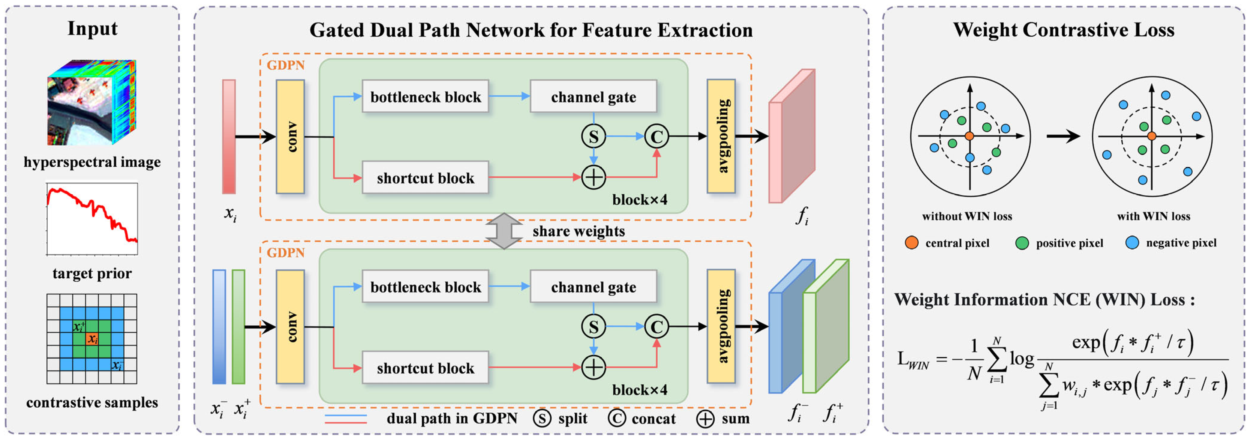
A new contrastive learning framework is investigated in this paper, aiming at enabling the model to learn the ability to distinguish spectral similarities and dissimilarities in an unsupervised manner. Specifically, the Gated Dual-Path Network reuses and explores features of the spectrum, allowing the model to capture the subtle and crucial differences between target and background, while the Weighted Information Noise Contrastive Estimation (WIN) loss simultaneously enhances the similarity of positive samples and increases the separation from negative samples.

(2)

We propose a physically interpretable spectral-level data augmentation based on pixel mixing. Unlike existing methods, it constructs positive and negative samples for each pixel, significantly reducing false negatives in contrastive learning. Refining sample pair selection minimizes the risk of mistakenly treating semantically related samples as negatives, thereby improving representation quality and enhancing the model’s ability to distinguish targets from backgrounds in high-dimensional spectral data. The code for this work will be made publicly available at https://github.com/liurongwhm (accessed on 28 June 2025) upon publication.

2. The Proposed Method

The flowchart depicting the proposed GDPNCL detector is presented in Figure 1, which consists of two main components:

(1)

Data Augmentation Module: This module employs spectral data augmentation to generate sample pairs for contrastive learning. By augmenting the spectral data, the model is provided with a diverse set of samples, enhancing the learning process and improving its robustness.

(2)

Network Module: This module is built upon the Gated Dual-Path Network (GDPN), which facilitates contrastive learning by extracting spectral features. It incorporates a weighted contrastive loss framework to promote similarity learning, and the GDPN efficiently captures the spectral characteristics, enabling the differentiation of negative samples under the constraint of the WIN loss, thereby optimizing the overall learning performance.

2.1. Spectral Data Augmentation

Contrastive learning aims to bring similar samples closer and push dissimilar ones apart in the feature space. Achieving this objective requires constructing meaningful positive and negative sample pairs, which largely rely on data augmentation techniques. Data augmentation generates diverse yet semantically consistent variations of the input data, enabling the creation of positive sample pairs that capture different perspectives of the same underlying entity. These variations help the model focus on invariant features essential for representation learning while disregarding superficial differences [45]. Additionally, data augmentation introduces variability into the training data, facilitating the generation of harder negative pairs, which are crucial for improving the discriminative power of the model. Moreover, it acts as an implicit regularizer, mitigating the risk of overfitting in the training data [46]. This is particularly important in scenarios where labeled data are scarce, such as HTD. Enriching the feature space and enhancing the diversity of the training set play a key role in improving the model’s generalization in contrastive learning [47]. Consequently, data augmentation emerges as an indispensable component for achieving high-quality representations. However, due to the absence of explicit labels, contrastive learning may occasionally generate false negatives during training by treating similar samples as dissimilar. This issue can hinder the model’s ability to learn accurate representations and degrade its performance in downstream tasks. To address this, methods such as Hard Negative Mining (HNM) are employed, where the model enhances its discriminative ability by selecting negative samples that are close to positive samples. Momentum Contrastive Learning (MoCo) [48] employs a slowly updated target representation to ensure more consistent negative samples. These approaches contribute to improving the quality of the learned representations by mitigating the impact of false negatives.

Despite the significant advances in contrastive learning, the application of the technique to HTD poses unique challenges. Unlike RGB images, hyperspectral data predominantly carries information through spectral curves rather than shape or texture in spatial. The main challenge lies in effectively learning differences from spectral information. Some efforts have been made to apply contrastive learning to HTD. For instance, Yang et al. [43] divide the hyperspectral data into odd and even bands using two trained encoders as data augmentation tools. While this method leverages a generative adversarial network to extract features for positive samples, it compromises half of the spectral information, potentially leading to suboptimal representation learning. Zhang et al. [49] combine the spatial transformer of hyperspectral patches with the spectra of the central pixel, which can be influenced by surrounding pixels. Another strategy used in [44] adds Gaussian noise to the image and treats positionally corresponding pixels as positive sample pairs. However, these augmentation methods often lack semantic relevance and fail to adequately capture real variability among pixels within the same class. Moreover, these methods frequently encounter the problem of false negative samples by treating different pixels and their augmentations within the same batch as negative samples.

In light of these limitations, our work aims to address these gaps by proposing a novel data augmentation strategy specifically designed for hyperspectral data. In contrast to previous approaches, our method considers semantic relevance to better capture the inherent variability in spectral data. The dual window strategy for HSIs was first proposed in [15], which generates an adaptive local background dictionary for test samples in sparse representation. The background dictionary varies for different test samples, making it challenging to collect as a training set in deep learning. To the best of our knowledge, no existing data augmentation method has yet utilized this strategy for contrastive learning. Inspired by the sparse representation technic, we develop a sliding dual window framework that separates the local area around each pixel into distinct regions. The inner window includes the target of interest, while the outer window, which excludes the targets, typically includes pixels different from the central pixel. This design enables the construction of positive and negative contrastive sample pairs, as pixels from the inner and outer windows are augmented accordingly. Figure 2 illustrates the dual concentric windows for contrastive sampling under different conditions.

Consider a hyperspectral image $\mathbf{Y}\in {\mathbb{R}}^{L\times h\times w}$, where L represents the number of spectral bands and $h\times w$ denotes the spatial dimensions. The inner and outer window sizes are defined as $w_{in}$ and $w_{out}$, respectively. The spectral data augmentation for a pixel $\mathbf{x}$ is performed as follows:

(1)

Synthesizing the embedded signal: using ( $w_{in}\times w_{in}-1$) pixels from the inner window, the embedded signal $\mathbf{t}$ is synthesized as follows:

$$\mathbf{t}=\sum _{i=1}^{w_{in} \times w_{in}-1}f\left(d_i\right)\times {\mathbf{s}}_{\mathbf{i}}$$

(1)

The weighting function f is an improved Tukey weight function [50], which provides a way to lessen the effect of pixels with excessively large differences and extreme data points, is defined as follows:

$$f\left(d_i\right)={(1-{({\displaystyle \frac{d_i}{k}})}^2)}^2$$

(2)

where the similarity $d_i$ between $\mathbf{x}$ and a neighboring pixel ${\mathbf{s}}_{\mathbf{i}}$ in the inner window is calculated as follows:

$$d_i=‖{\mathbf{s}}_{\mathbf{i}}-\mathbf{x}‖$$

(3)

In Equation (2), $k=\max \left(d_i\right)$ normalizes the weights within the range [0, 1]. This ensures that pixels less similar to x are assigned lower weights. The normalization helps prevent the signal from being overly disturbed by extreme or background pixels with large dissimilarity. Subsequently, the embedded signal is prepared, considering neighbor pixels while avoiding large fluctuations.

(2)

Constructing positive samples: After synthesizing the embedded signal from the inner window, the positive sample ${\mathbf{x}}^{+}$ is constructed by incorporating a certain proportion $\theta$ of the signal into the central pixel:

$${\mathbf{x}}^{+}=(1-\theta )\times \mathbf{x}+\theta \times \mathbf{t}$$

(4)

where $\mathbf{x}$ is the reflectance of the central pixel, and $\mathbf{t}$ is the synthesized signal by Equation (1). $\theta$ is the parameter to control the variability of positive samples. A small $\theta$ yields positive samples that are highly similar to the central pixel. In contrast, a large $\theta$ introduces greater dissimilarity, which may compromise the model’s capacity to accurately distinguish positive from negative samples. The synthetic positive spectrum is constructed by emulating the spectral variability of the inner window pixels. Step (2) generates a signal that incorporates scattering from nearby pixels. In step (3), a specific proportion ensures that the central pixel remains the foundation of the positive sample. This process generates a positive sample that captures spectral variability while preserving class consistency.

(3)

Selecting negative samples from the outer window: For each pixel in the outer window, its Euclidean distance to the central pixel is calculated. The pixel with the maximum distance is chosen as the negative sample:

$${\mathbf{x}}^{-}=\underset{n_i\in N}{\mathrm{argmax}}‖{\mathbf{n}}_{\mathbf{i}}-\mathbf{x}‖$$

(5)

where $N$ is the pixel set in the outer window, containing ${(w_{out}\times w_{out}-w}_{in}\times w_{in})$ pixels. This strategy identifies hard negative samples, i.e., pixels from different landcover types near the central pixel, which are particularly challenging for the model to distinguish from positive samples. Incorporating such hard negative samples enhances the ability to learn discriminative features effectively.

2.2. Gated Dual-Path Network

For HSIs, spectral signatures play a more crucial role in identifying substances compared to spatial information in 3D data patches, which can be influenced by mixed neighboring pixels. However, it remains challenging to extract both global and local features from the spectral data of a single pixel. Traditional down-sampling in networks further degrades the already limited spectral information, neglecting crucial local differences essential for separating targets from similar backgrounds and potentially leading to overfitting on training data. The Residual Network (ResNet) has been developed to address the issue of information reduction in feature maps across layers. While this approach effectively prevents information loss and overfitting by reusing features, ResNet struggles to explore new features, thereby limiting its capacity to capture fine-grained spectral details necessary for distinguishing targets from backgrounds. In contrast, Densely Connected Networks (DenseNet) excel in exploring new features by connecting each layer to every subsequent layer, promoting comprehensive feature extraction. Nonetheless, DenseNet may introduce feature redundancy, particularly in hyperspectral data, where adjacent bands tend to exhibit high correlation.

To overcome these limitations, the proposed method integrates ResNet and DenseNet into a dual-path design that leverages their respective strengths. Additionally, the channel gate mechanism balances the features extracted from DenseNet, ensuring that only the most relevant information is retained for representation learning. Both the residual-like and dense-like paths are designed with bottleneck blocks, each consisting of three convolutional layers (1 × 1, 1 × 3, and 1 × 1 convolutional layers) and a shortcut block (1×1 convolutional layer). The process of the GDPN block $E_{GDPN}(\cdot )$ is described as follows:

(1)

Residual-like path: The residual path ensures that important spectral features are preserved as the network deepens. This is achieved by reusing previously extracted information, a strategy that enhances the ability of the network to extract features from the input data. For the m-th block in the GDPN encoder, the output from the residual-like path is given using the following:

$${\mathbf{u}}_{\mathbf{m}}=R\left({\mathbf{x}}_{\mathbf{m}-1}\right)$$

(6)

where $R$ is the sum of the bottleneck block and the shortcut block, following the standard ResNet formulation.

(2)

Dense-like path and channel gate: The dense path focuses on exploring new features by capturing local discriminative spectral information, helping the network identify subtle spectral differences between targets and backgrounds. However, the dense-like path may introduce irrelevant features, potentially accumulating bias during the learning process. To address this, we propose assigning weights to the features derived from the dense path through the learnable channel gate ${\mathbf{a}}_{\mathbf{m}}$. The gate automatically learns channel-wise weights using a fully-connected layer, based on the current features, suppressing less relevant channels before the next DPN block. This ensures that only the most informative features for representation learning contribute significantly.

Features generated by the dense-like path (${\mathbf{y}}_{\mathbf{l}}$) are passed through a fully connected layer ${\mathbf{W}}_{\mathbf{f}\mathbf{c}}$ with a sigmoid activation function $\sigma$, producing a gate vector ${\mathbf{a}}_{\mathbf{l}}$:

$${\mathbf{y}}_{\mathbf{m}}=D\left({\mathbf{x}}_{\mathbf{m}-1}\right)$$

(7)

$${\mathbf{a}}_{\mathbf{m}}=\sigma \left[{{\mathbf{W}}_{\mathbf{f}\mathbf{c}}}^{\mathbf{T}}{\mathbf{y}}_{\mathbf{m}}\right]$$

(8)

where $D$ represents the dense-like path. The gate features are then calculated as follows:

$${\mathbf{v}}_{\mathbf{m}}={\mathbf{y}}_{\mathbf{m}}⨂{\mathbf{a}}_{\mathbf{m}}$$

(9)

where $⨂$ denotes channel-wise multiplication. The outputs of the residual-like and dense-like paths are combined to form the final output of $m-\mathrm{t}\mathrm{h}$ block:

$${\mathbf{x}}_{\mathbf{m}}=sum\left({\mathbf{v}}_{\mathbf{m}}+{\mathbf{u}}_{\mathbf{m}}\right)$$

(10)

The function $sum(·)$ in (10) includes both the summation and concatenate operations. The results of the same channel as ResNet in the output ${\mathbf{v}}_{\mathbf{l}}$ are added to ${\mathbf{u}}_{\mathbf{l}}$ and the new features generated by DenseNet are concatenated with this summation.

The spectral contrastive encoder $h\left(x\right)$ is designed to effectively capture both global and local spectral features. First, the 1-D spectral data is expanded using a convolution operation. To capture local distinctive characteristics of spectral data, such as peaks, troughs, and abrupt changes in spectral curves, the convolutional kernel size and stride are set to 1 × 7 and 2, respectively.

$${\mathbf{x}}_0={conv}_{1\times 7}\left(\mathbf{x}\right)$$

(11)

The convolutional output is then fed into $m$ dual-path blocks (with $m=4$ in this design), where the residual-like path ensures feature reuse while the dense-like path explores new representations. To enhance feature selection, a channel gate mechanism assigns different weights to features from the dense path, prioritizing those most beneficial:

$${\mathbf{x}}_{\mathbf{m}}=E_{GDPN}\left({\mathbf{x}}_{\mathbf{m}-1}\right)$$

(12)

Finally, the extracted features undergo average pooling to generate the final representation for loss calculation, ensuring a well-balanced and discriminative spectral encoding.

$$\mathbf{f}=avgpool\left({\mathbf{x}}_{\mathbf{m}}\right)$$

(13)

2.3. Loss Function

In general, a contrastive loss [43] is minimized to promote similarity among positive sample pairs while ensuring that all negative samples remain dissimilar. Conventional contrastive learning methods form negative pairs between augmented samples from different locations. In contrast, our approach assigns each sample its own positive and negative pairs. As a result, the similarity calculation for negative samples varies across different samples within a batch. The relationship between the current sample and other samples in the batch can be used as a weight for the dissimilarity of negative samples. To further enhance the proximity of positive samples, we improve the Information Noise Contrastive Estimation (InfoNCE) loss [51] and propose the Weighted Information NCE (WIN) loss, defined as follows:

$$L_{WIN}=-{\displaystyle \frac{1}{N}}\sum _{i=1}^{N}log{\displaystyle \frac{exp({\mathbf{f}}_{\mathbf{i}}\ast {\mathbf{f}}_{\mathit{i}}^{+}/\tau )}{\sum _{j=1}^N{w}_{i,j}\ast exp({\mathbf{f}}_{\mathbf{j}}\ast {\mathbf{f}}_{\mathbf{j}}^{-}/\tau )}}$$

(14)

$$w_{i,j}=‖{\mathbf{f}}_{\mathbf{i}}-{\mathbf{f}}_{\mathbf{j}}‖$$

(15)

where N denotes the batch size, $\tau$ is the temperature hyperparameter which is set to 0.7, and ${\mathbf{f}}_{\mathbf{i}}$, ${{\mathbf{f}}_{\mathbf{i}}}^{+}$ refer to the output of $\mathbf{x}$ and its augmentation ${\mathbf{x}}^{+}$ through the encoder, respectively. Analogously, ${\mathbf{f}}_{\mathbf{j}}$ and ${{\mathbf{f}}_{\mathbf{j}}}^{-}$ are negative sample features in the batch. The loss function computes the sum of one positive sample and N negative samples, with the contribution of each negative sample being adjusted according to its proximity to the current sample ${\mathbf{x}}_{\mathbf{i}}$. If ${\mathbf{x}}_{\mathbf{j}}$ is closer to ${\mathbf{x}}_{\mathbf{i}}$, it is more likely to belong to the same class, and its contribution to the negative term is reduced accordingly. By assigning a small weight to similar samples, the contribution of their negative counterparts in the calculation would decrease, which improves the similarity between positive samples. The samples of homogeneous classes within a batch are not regarded as negative samples during training under the constraint of WIN loss. Conversely, the dissimilarities between negative samples are amplified, thereby enabling the model to discern homogeneous pixels with greater precision.

2.4. Pixel Detection

Once training is complete, the well-trained network encoder extracts discriminative features from HSIs. Given a prior spectral reference ${\mathbf{x}}_{\mathbf{*}}$, the target detection score is calculated using cosine similarity. The final output of GDPNCL is as follows:

$$D_{GDPNCL}\left(\mathbf{x}\right)={\displaystyle \frac{g\left(\mathbf{x}\right)·{g\left({\mathbf{x}}_{\mathbf{*}}\right)}^T}{‖g\left(\mathbf{x}\right)‖·‖g\left({\mathbf{x}}_{\mathbf{*}}\right)‖}}$$

(16)

where $g\left(·\right)$ is the trained encoder with the GDPN backbone, which has learned discriminative contrastive spectral characteristics to distinguish targets from the background. The overall procedure of the proposed GDPNCL algorithm is summarized in Algorithm 1.

Algorithm 1. GDPNCL for Hyperspectral Target Detection

Input: hyperspectral data $\mathbf{Y}\in {\mathbb{R}}^{L\times h\times w}$, target samples ${\mathbf{x}}^{\mathit{*}}\in {\mathbb{R}}^{L\times 1}$, parameters $w_{in}$, $w_{out}$, $\theta$ and $\tau$.

Output: Two-dimensional plot of detection results.

Spectral Data Augmentation:

For each x in image $\mathbf{Y}$,               (1) construct positive sample ${\mathbf{x}}^{+}$ of pixel $\mathbf{x}$ via Equations (1)–(4)               (2) select negative sample ${\mathbf{x}}^{-}$ of pixel $\mathbf{x}$ via Equation (5)       End for

Contrastive learning:

Training the GDPN network using contrastive samples ${\mathbf{x}}^{+}$ and ${\mathbf{x}}^{-}$ generated from data augmentation with WIN loss in Equations (14) and (15)

Target Detection for HSI:       Calculate the target feature via GDPN network $g\left(·\right)$.

For each x in image $\mathbf{Y}$,

(1) calculate the pixel feature via GDPN network $g\left(·\right)$.

(2) obtain detection statistics via Equation (16).

End for

The proposed method signifies a substantial enhancement over existing methodologies due to its integration of a sample augmentation approach that considers the spectral semantic meaning for self-supervised contrastive learning. This approach fully leverages both global and local spectral information in the feature extraction network to capture the similarities and differences between spectral pairs. Moreover, the WIN loss further aids in mitigating the problem of false negatives, enhancing the dissimilarity between negative samples in the batch. The proposed methodology enables the model to learn more discriminative representations for heterogeneous spectra, thereby improving the separation of background and targets in HSI.

3. Experiments and Analysis

In this section, extensive experiments conducted on four real-world datasets are used to validate the effectiveness of the GDPNCL detector. First of all, the hyperspectral datasets are described in detail. Then, the target detection performance is compared against state-of-the-art methods, including various representation-based and deep network-based target detection algorithms. Subsequently, several parameter analyses are provided. Finally, the ablation studies are conducted to ascertain the validity of the model.

3.1. Data Description

The first and second datasets capture urban scenes from the Texas Coast and Gainesville. The Urban-1 dataset has 204 spectral bands with a spatial resolution of 17.2 m, while the Urban-2 dataset has 191 spectral bands and a spatial resolution of 3.5 m. Both datasets cover wavelengths from 0.4 to 2.5 µm. The third dataset was acquired in San Diego, CA, USA, by AVIRIS, with a spatial resolution of 3.5 m. It consists of 224 spectral bands covering wavelengths from 0.37 to 2.5 µm. After removing poor-quality bands, 189 bands were retained for experiments. The fourth dataset was collected in the SHARE 2012 data campaign in Avon, NY. It comprises 200 × 200 pixels with 360 bands. The spatial resolution is 1 m, and the spectral resolution is 5 nm.

Table 1. Detailed information about four datasets. “/” means the information is unknown.

Dataset	Number of Bands	Sensor	Image Size	Spatial Resolution	Target	Target Proportion
Urban-1	204	AVIRIS	100 × 100	17.2 m/pixel	/	0.17%
Urban-2	191	AVIRIS	100 × 100	3.5 m/pixel	boat	0.13%
AVIRIS	189	AVIRIS	100 × 100	3.5 m/pixel	plane	0.15%
RIT Campus	360	ProSpecTIR	200 × 200	1 m/pixel	red panel	0.20%

provides detailed information on these datasets.

3.2. Experimental Settings

3.2.1. Performance Metrics

Three widely recognized metrics are adopted to evaluate the performance of the GDPNCL for HTD: the receiver operating characteristic (ROC) curve, the area under the ROC curve (AUC), and the target-background separability (TBS) map.

The ROC curve provides insight into performance at various thresholds by plotting the probability of detection (PD) against the false alarm rate (FAR) under fixed conditions. PD is calculated as the ratio of detected target pixels to true target pixels, while FAR is the ratio of falsely detected pixels to total image pixels. In general, an ROC curve closer to the upper left corner indicates better performance.

The AUC derived from the ROC curve provides a quantitative measure of detection efficiency. It represents the area under the ROC curve, with values ranging from 0 to 1 [52]. A higher AUC value indicates superior detector capability.

The TBS map assesses target-background separability through box plots, with the ordinate representing the normalized detection statistic [53,54,55]. Pixels are divided into either target or background based on their labels. The normalized detection statistics are then visualized as box plots, where greater separation between the target and background distributions indicates improved target discriminability while minimizing background interference.

3.2.2. Comparison Detectors and Parameter Settings

Seven state-of-the-art HTD algorithms are deployed for performance comparison: one classical detector (CEM [11]), two representation learning-based detectors (SRBBH [16] and SASTD [56]), and five deep learning-based detectors (CSTTD [32], MCLT [44], TSTTD [35], and MLSN [37]). To maintain a fair comparison, all methods are applied to different datasets using the recommended parameter settings from their respective papers. For the proposed GDPNCL method, the dual window sizes are set to 7 and 25, while the implantation proportion is fixed at 0–30% for all four HSIs. All experiments were conducted on a 11th Gen Intel(R) Core (TM) i9-11900K CPU machine running a 64-bit Windows 11 Operating System (OS) (Intel, Santa Clara, CA, USA).

3.3. Detection Performance

As illustrated in Figure 3, the color maps of detection results for all detectors across the four HSIs reveal the performance of various detection methods. For the Urban-1 dataset, CEM, SASTD, TSTTD, and MSLN exhibit poor detection performance, capturing only a limited number of target pixels. The SRBBH detector fails to detect one of the target objects. In contrast, CSTTD and the proposed GDPNCL detector successfully detect targets at different locations. The Urban-2 dataset contains numerous small-sized targets. CEM and SRBBH introduce noise, while SASTD struggles to achieve satisfactory detection. Although CSTTD demonstrates strong performance with effective background suppression, it produces false alarms on the right side. The MCLT detector struggles to separate targets from the background, while TSTTD and MLSN yield incomplete detections. GDPNCL overcomes these challenges, delivering more accurate and reliable detection results. For the AVIRIS dataset, several deep learning-based methods (CSTTD, MCLT, TSTTD, MLSN) achieve decent detection but miss certain target pixels. SASTD generates excessively high detection values, complicating target identification. GDPNCL effectively detects all three planes, though its background suppression capability is slightly weaker than CSTTD, particularly in the lower-left corner of the image. For the RIT Campus dataset, the classic CEM detector performs well but introduces noise. The GDPNCL demonstrates significant advantages over competing methods, while SASTD, CSTTD, and MCLT fail to highlight targets. TSTTD also encounters the challenge of omitting some target pixels.

The comparison of ROC curves is displayed in Figure 4. As shown, GPNCL achieves optimal ROC curves across all four hyperspectral datasets, consistently maintaining low false alarm rates and high detection probabilities. In the Urban-1, Urban-2, and RIT Campus datasets, GDPNCL in the red curve maintains low false alarms and high detection probabilities, outperforming other detectors at a false alarm rate of 1 × 10⁻². The SASTD and MCLT perform poorly across the Urban-1 and RIT Campus datasets. Although the CSTTD performs well in the AVIRIS dataset, its performance drops significantly in the RIT Campus dataset. In contrast, GDPNCL maintains a consistently outstanding ROC across all datasets, demonstrating superior robustness. This reliability is due to the model’s ability to capture both local and global spectral information, making it less susceptible to variations in spatial resolution.

Table 2. AUC comparison of different methods across four datasets. (Highest: bold & underlined; second highest: bold).

Dataset	Urban-1	Urban-2	AVIRIS	RIT Campus
CEM	0.6775	0.9836	0.9849	0.9972
SRBBH	0.8684	0.7792	0.7800	0.7465
SASTD	0.8585	0.9404	0.9535	0.8253
CSTTD	0.9946	0.9932	0.9992	0.7788
MCLT	0.6613	0.9939	0.9867	0.7101
TSTTD	0.9900	0.9880	0.9953	0.9821
MLSN	0.9767	0.9291	0.9918	0.9888
Proposed	0.9957	0.9956	0.9974	0.9983

lists the AUC values for different detectors, with the highest values in bold and underlined and the second highest values in bold. GDPNCL achieves AUC values exceeding 0.995 on all datasets. Representation learning-based methods, such as SRBBH and SASTD, are highly sensitive to hyperparameters and lack clear guidelines for real-world applications. Moreover, both methods perform poorly on the RIT Campus dataset, likely due to background contamination affecting the dictionary-based representation. While CSTTD performs well on the first three datasets, its accuracy drops significantly on the RIT Campus dataset because it relies on generating a random vector based on a Gaussian distribution to serve as target spectral samples—a strategy that lacks robustness across different datasets.

The TBS maps are presented in Figure 5, demonstrating GDPNCL’s superior ability to distinguish targets from the background across all four datasets. For the Urban-1 dataset, GDPNCL achieves a well-defined separation between target and background detection statistics, outperforming other detectors. SASTD, MCLT, and MLSN fail to effectively differentiate targets from the background, reducing their effectiveness for background suppression. CSTTD also performs well on this dataset. For the Urban-2 dataset, GDPNCL demonstrates superior capability in restricting target statistics within a narrow range, whereas CSTTD, MCLT, and TSTTD exhibit some overlap due to target distribution variations. Similarly, for the AVIRIS dataset, the GDPNCL maintains its advantage and obtains the suboptimal target-background separation, further strengthening its reliability. For the RIT Campus dataset, despite minor limitations in background suppression at lower values, it still provides a superior separation between target and background classes, further validating its robustness and generalization capabilities across different datasets. Additionally, GDPNCL reduces target-background overlap in box plots, thereby minimizing false positives and false negatives. The effectiveness of GDPNCL stems from its spectrally aware data augmentation, which generates positive samples while preserving spectral variability. This approach reinforces the constraint on the distribution of the target statistic and outperforms other deep learning methods in hyperspectral target detection.

The runtimes of deep learning-based methods on four datasets are presented in

Table 3. Running time (in seconds) of deep learning methods for four datasets.

	CSTTD		MCLT		TSTTD		MLSN		GDPNCL
	Train	Test	Train	Test	Train	Test	Train	Test	Train	Test
Urban-1	593.04	0.27	65.57	0.72	350.02	1.10	637.37	13.08	46.61	0.43
Urban-2	677.85	0.28	59.98	0.69	349.51	1.10	667.76	12.80	52.56	0.11
AVIRIS	419.35	0.26	59.73	0.66	348.89	1.13	662.36	12.24	44.47	0.39
RIT Campus	842.98	0.42	582.23	6.82	603.74	3.45	1126.45	72.84	222.77	15.48

. Among them, the meta-learning method MLSN reports only the fine-tuning training time. Compared with the other deep learning-based methods, the proposed GDPNCL significantly reduces runtime, particularly during training, due to its use of one-dimensional spectral data as network input.

Overall, the proposed GDPNCL demonstrates exceptional performance and consistency, achieving superior AUC scores, ROC curves, and target-background separability across all datasets. It effectively captures spectral features in complex data by self-supervised contrastive learning and enhances the ability to distinguish subtle differences between targets and backgrounds. The results validate the effectiveness of the GDPNCL in target detection, consistently outperforming state-of-the-art methods across diverse real-world datasets. These findings underscore the robustness, reliability, and practical applicability of the proposed method for HTD tasks.

3.4. Analysis of Parameters

Selecting appropriate positive and negative samples is crucial for balancing the discrimination of similar spectral features and minimizing the influence of noise and irrelevant variations. This section examines the impact of two key data augmentation parameters: window size and implantation proportion.

3.4.1. Analysis of Window Size

In data augmentation, positive and negative samples are constructed based on the assumption that spatially adjacent pixels in HSIs exhibit spectral similarity. However, the range of similarity is not fixed. Therefore, an experimental evaluation of the optimal window size for distinguishing similar and dissimilar samples is necessary. If the inner window is too small, the positive sample pairs become overly similar, leading to overfitting. Conversely, if the inner window is too large, the sample pairs may become too different, making it difficult for the model to learn effective representations. To analyze the influence of window size, experiments were conducted with inner window sizes of 5, 7, 9, 11, and 13, and outer window sizes of 17, 21, 25, 29, and 33. Since pixels in the outer window are candidates for the most different one, the interval of the outer size is set as 4. The corresponding results are presented in Figure 6.

In general, the AUC results show little variation across different dual-window sizes, especially for the Urban-1 dataset. Unlike representation learning-based methods, which directly collect pixels within the dual window to construct a dictionary, our method uses these pixels to augment the central pixel. This explains its robustness to variations in window size, even for targets with varying shapes. For the Urban-2, AVIRIS, and RIT Campus datasets, AUC values tend to decrease when the outer window is too small, as negative samples within this range exhibit insufficient spectral differences. Based on these observations, we recommend setting the inner window size to 7 and the outer window size to 25 for the proposed GDPNCL method.

3.4.2. Analysis of the Proportion of Implantation

Since the weighted sum of spectra from the inner window is incorporated into the center pixel to synthesize a new signal, the proportion of implantation directly impacts the variability of positive samples. If the positive sample deviates excessively from the central pixel, indicating a high degree of dissimilarity, the loss function may fail to extract meaningful features that reflect actual spectral similarities and differences. This can lead to misclassification, where background pixels are falsely detected as targets. Conversely, if the difference between the center pixel and the positive sample is excessively small, the model may be prone to overfit. This can hinder the model’s ability to effectively handle spectral variability caused by noise or mixed pixels, thereby reducing the accuracy of target detection.

To evaluate the sensitivity of the model to the implantation proportion $\theta$, experiments were conducted with values of 5%, 10%, 15%, 20%, 25%, 30%, 35%, 40%, and 45%. The AUC results under different implantation proportions are displayed in Figure 7. For Urban-2 and AVIRIS datasets, AUC values decrease slightly when $\theta$ is less than 25%, while the Urban-1 dataset exhibits almost no fluctuation. An anomalous trend is observed in the RIT Campus dataset, where AUC peaks at 10% and exhibits a sharp decline beyond 35%. This phenomenon can be attributed to the manual panel targets, which are closely spaced within the dataset. Excessive implantation leads to a disruption of the spectral characteristics of the panels. However, the impact of implantation remains limited, as the spectral characteristics of neighboring pixels within the inner window inherently resemble those of the central pixel. In light of these findings, we recommend setting $\theta$ to 30% for stable performance across different datasets.

3.5. Analysis of the Model and WIN Loss

To validate the effectiveness of the GDPN encoder and WIN loss in the proposed GDPNCL detector, two ablation studies are conducted across all four datasets: (1) a comparison of the GDPN encoder with the ResNet-50 baseline and (2) an evaluation of the WIN loss against the InfoNCE loss under the GDPN framework.

The AUC results of the ablation experiments are shown in Figure 8. As illustrated in Figure 8a, the GDPN encoder significantly improves performance over the ResNet-50 baseline, with AUC increases exceeding 0.05 for the Urban-1, AVIRIS, and RIT Campus datasets. This demonstrates the effectiveness of the GDPN encoder in extracting local and global discriminative features.

On the basis of the proposed data augmentation strategy, the WIN loss further enhances performance by adaptively adjusting sample weights in similarity calculations within a batch, thereby strengthening the model’s ability to capture meaningful relationships between positive samples. The combined effect of data augmentation and the loss function is demonstrated through ablation experiments, as illustrated in Figure 8b. As shown, the data augmentation and WIN loss both have a notable positive effect on the Urban-1, Urban-2, and RIT Campus datasets. By considering the spatial neighbors of pixels when constructing positive and negative pairs, the strategy enables more effective contrastive learning, especially in scenes with small and complex targets. For the AVIRIS dataset, applying the dual-window strategy without the WIN loss results in a decline in detection performance, which may be attributed to the presence of large homogeneous regions in the image. In such cases, the dual-window augmentation may introduce false negative samples. The RIT Campus dataset benefits most from WIN loss, likely due to its complex scene with diverse land cover types, where precise target detection poses a particular challenge. These results confirm that both the GDPN encoder and the WIN loss play crucial roles in significantly improving detection accuracy.

4. Discussion

Owing to the GDPN network’s ability to extract discriminative spectral features independent of surrounding interference, the proposed method achieves superior detection performance in complex backgrounds. This is particularly evident on challenging datasets such as RIT Campus, where baseline methods exhibit limited robustness. The dual-window augmentation strategy can accommodate variations in target size to a certain extent, except in cases where the target entirely covers the outer window. However, it may still generate false-negative samples when applied to scenes with large homogeneous background regions, potentially degrading detection performance in hyperspectral images with such characteristics. Another limitation is the substantial memory usage during the training stage, which may make the method unsuitable for lightweight tasks.

Although the method effectively extracts discriminative spectral features, it remains limited in its use of spatial contextual information, which can provide valuable complementary cues for spectral discrimination. In future work, we aim to incorporate transformer-based spatial-contextual modeling to further enhance the discriminability of targets that deviate from the background.

5. Conclusions

In this work, we propose a novel detection framework for HTD, named Gate Dual-Path Network Contrastive Learning (GDPNCL for short). By leveraging self-supervised contrastive learning, GDPNCL reduces the dependence of deep learning models on prior information. A tailored data augmentation strategy is proposed to construct samples for network training from the HSI to be detected. Furthermore, a spectral contrastive learning framework is designed to enhance the model’s ability to distinguish spectral similarities and differences effectively. Extensive experiments conducted on four real-world datasets confirm the effectiveness of the model. The detection results demonstrate that the proposed GDPNCL outperforms state-of-the-art detection methods, offering both superior accuracy and robustness. Further work will be conducted on exploiting contrastive information on multiple datasets through transfer learning theory to achieve realistic and higher-quality training samples.

References

1. Green, R.O.; Eastwood, M.L.; Sarture, C.M.; Chrien, T.G.; Aronsson, M.; Chippendale, B.J.; Faust, J.A.; Pavri, B.E.; Chovit, C.J.; Solis, M.; et al. Imaging spectroscopy and the Airborne Visible/Infrared Imaging Spectrometer (AVIRIS). Remote Sens. Environ. 1998, 65, 227–248. [Google Scholar] [CrossRef]
2. Manolakis, D.; Shaw, G. Detection algorithms for hyperspectral imaging applications. IEEE Signal Process. Mag. 2002, 19, 29–43. [Google Scholar] [CrossRef]
3. Landgrebe, D. Hyperspectral image data analysis. IEEE Signal Process. Mag. 2002, 19, 17–28. [Google Scholar] [CrossRef]
4. Bioucas-Dias, J.M.; Plaza, A.; Camps-Valls, G.; Scheunders, P.; Nasrabadi, N.; Chanussot, J. Hyperspectral Remote Sensing Data Analysis and Future Challenges. IEEE Geosci. Remote Sens. Mag. 2013, 1, 6–36. [Google Scholar] [CrossRef]
5. Liu, J.; Hou, Z.; Li, W.; Tao, R.; Orlando, D.; Li, H. Multipixel Anomaly Detection with Unknown Patterns for Hyperspectral Imagery. IEEE Trans. Neural Netw. Learn. Syst. 2022, 33, 5557–5567. [Google Scholar] [CrossRef] [PubMed]
6. Hu, X.; Ou, J.; Zhou, M.; Hu, M.; Sun, L.; Qiu, S.; Li, Q.; Chu, J. Spatial-spectral identification of abnormal leukocytes based on microscopic hyperspectral imaging technology. J. Innov. Opt. Health Sci. 2020, 13, 2050005. [Google Scholar] [CrossRef]
7. Sneha; Kaul, A. Hyperspectral imaging and target detection algorithms: A review. Multimed. Tools Appl. 2022, 81, 44141–44206. [Google Scholar] [CrossRef]
8. Manolakis, D.; Marden, D.; Shaw, G.A. Hyperspectral image processing for automatic target detection applications. Linc. Lab. J. 2003, 14, 79–116. [Google Scholar]
9. Kraut, S.; Scharf, L.L.; Butler, R.W. The adaptive coherence estimator: A uniformly most-powerful-invariant adaptive detection statistic. IEEE Trans. Signal Process. 2005, 53, 427–438. [Google Scholar] [CrossRef]
10. Manolakis, D.; Lockwood, R.; Cooley, T.; Jacobson, J. Is there a best hyperspectral detection algorithm? In Algorithms and Technologies for Multispectral, Hyperspectral, and Ultraspectral Imagery XV; SPIE: Orlando, FL, USA, 2009; Volume 7334, pp. 13–28. [Google Scholar]
11. Farrand, W.H.; Harsanyi, J.C. Mapping the distribution of mine tailings in the Coeur d’Alene River Valley, Idaho, through the use of a constrained energy minimization technique. Remote Sens. Environ. 1997, 59, 64–76. [Google Scholar] [CrossRef]
12. Chang, C.I. Orthogonal subspace projection (OSP) revisited: A comprehensive study and analysis. IEEE Trans. Geosci. Remote Sens. 2005, 43, 502–518. [Google Scholar] [CrossRef]
13. Jiao, X.; Chang, C.I. Kernel-based constrained energy minimization (K-CEM). In Proceedings of the Algorithms and Technologies for Multispectral, Hyperspectral, and Ultraspectral Imagery XIV; SPIE: Bellingham, WA, USA, 2008; Volume 6966, pp. 523–533. [Google Scholar]
14. Kwon, H.; Nasrabadi, N.M. Kernel spectral matched filter for hyperspectral imagery. Int. J. Comput. Vis. 2007, 71, 127–141. [Google Scholar] [CrossRef]
15. Chen, Y.; Nasrabadi, N.M.; Tran, T.D. Sparse representation for target detection in hyperspectral imagery. IEEE J. Sel. Top. Signal Process. 2011, 5, 629–640. [Google Scholar] [CrossRef]
16. Zhang, Y.; Du, B.; Zhang, L. A sparse representation-based binary hypothesis model for target detection in hyperspectral images. IEEE Trans. Geosci. Remote Sens. 2014, 53, 1346–1354. [Google Scholar] [CrossRef]
17. Liu, R.; Wu, J.; Zhu, D.; Du, B. Weighted Discriminative Collaborative Competitive Representation with Global Dictionary for Hyperspectral Target Detection. IEEE Trans. Geosci. Remote Sens. 2024, 63, 1–13. [Google Scholar] [CrossRef]
18. Zhao, X.; Li, W.; Zhao, C.; Tao, R. Hyperspectral Target Detection Based on Weighted Cauchy Distance Graph and Local Adaptive Collaborative Representation. IEEE Trans. Geosci. Remote Sens. 2022, 60, 1–13. [Google Scholar] [CrossRef]
19. Zhu, D.; Du, B.; Hu, M.; Dong, Y.; Zhang, L. Collaborative-guided spectral abundance learning with bilinear mixing model for hyperspectral subpixel target detection. Neural Netw. 2023, 163, 205–218. [Google Scholar] [CrossRef]
20. Zhao, X.; Liu, K.; Gao, K.; Li, W. Hyperspectral time-series target detection based on spectral perception and spatial-temporal tensor decomposition. IEEE Trans. Geosci. Remote Sens. 2023, 61, 5520812. [Google Scholar] [CrossRef]
21. Jiao, C.; Yang, B.; Wang, Q.; Wang, G.; Wu, J. Discriminative Multiple-Instance Hyperspectral Subpixel Target Characterization. IEEE Trans. Geosci. Remote Sens. 2022, 60, 5521420. [Google Scholar] [CrossRef]
22. Du, J.; Li, Z. A hyperspectral target detection framework with subtraction pixel pair features. IEEE Access 2018, 6, 45562–45577. [Google Scholar] [CrossRef]
23. Gao, H.; Zhang, Y.; Chen, Z.; Xu, F.; Hong, D.; Zhang, B. Hyperspectral Target Detection via Spectral Aggregation and Separation Network With Target Band Random Mask. IEEE Trans. Geosci. Remote Sens. 2023, 61, 5515516. [Google Scholar] [CrossRef]
24. Qin, H.; Xie, W.; Li, Y.; Du, Q. HTD-VIT: Spectral-Spatial Joint Hyperspectral Target Detection with Vision Transformer. In Proceedings of the IGARSS 2022–2022 IEEE International Geoscience and Remote Sensing Symposium, Kuala Lumpur, Malaysia, 17–22 July 2022; pp. 1967–1970. [Google Scholar]
25. Zhang, G.; Zhao, S.; Li, W.; Du, Q.; Ran, Q.; Tao, R. HTD-net: A deep convolutional neural network for target detection in hyperspectral imagery. Remote Sens. 2020, 12, 1489. [Google Scholar] [CrossRef]
26. Shen, D.; Ma, X.; Kong, W.; Liu, J.; Wang, J.; Wang, H. Hyperspectral Target Detection Based on Interpretable Representation Network. IEEE Trans. Geosci. Remote Sens. 2023, 61, 1–16. [Google Scholar] [CrossRef]
27. Dong, W.; Wu, X.; Qu, J.; Gamba, P.; Xiao, S.; Vizziello, A.; Li, Y. Deep spatial–spectral joint-sparse prior encoding network for hyperspectral target detection. IEEE Trans. Cybern. 2024, 54, 7780–7792. [Google Scholar] [CrossRef] [PubMed]
28. Xu, S.; Geng, S.; Xu, P.; Chen, Z.; Gao, H. Cognitive fusion of graph neural network and convolutional neural network for enhanced hyperspectral target detection. IEEE Trans. Geosci. Remote Sens. 2024, 62, 1–15. [Google Scholar] [CrossRef]
29. Li, Y.; Shi, Y.; Wang, K.; Xi, B.; Li, J.; Gamba, P. Target detection with unconstrained linear mixture model and hierarchical denoising autoencoder in hyperspectral imagery. IEEE Trans. Image Process. 2022, 31, 1418–1432. [Google Scholar] [CrossRef]
30. Xie, W.; Lei, J.; Yang, J.; Li, Y.; Du, Q.; Li, Z. Deep latent spectral representation learning-based hyperspectral band selection for target detection. IEEE Trans. Geosci. Remote Sens. 2019, 58, 2015–2026. [Google Scholar] [CrossRef]
31. Li, Y.; Qin, H.; Xie, W. HTDFormer: Hyperspectral Target Detection Based on Transformer With Distributed Learning. IEEE Trans. Geosci. Remote Sens. 2023, 61, 1–15. [Google Scholar] [CrossRef]
32. Yang, Q.; Wang, X.; Chen, L.; Zhou, Y.; Qiao, S. CS-TTD: Triplet Transformer for Compressive Hyperspectral Target Detection. IEEE Trans. Geosci. Remote Sens. 2024, 62, 5533115. [Google Scholar] [CrossRef]
33. Zhu, D.; Du, B.; Zhang, L. Two-stream convolutional networks for hyperspectral target detection. IEEE Trans. Geosci. Remote Sens. 2020, 59, 6907–6921. [Google Scholar] [CrossRef]
34. Gao, Y.; Feng, Y.; Yu, X. Hyperspectral Target Detection with an Auxiliary Generative Adversarial Network. Remote Sens. 2021, 13, 4454. [Google Scholar] [CrossRef]
35. Jiao, J.; Gong, Z.; Zhong, P. Triplet spectralwise transformer network for hyperspectral target detection. IEEE Trans. Geosci. Remote Sens. 2023, 61, 1–17. [Google Scholar] [CrossRef]
36. Tian, Q.; He, C.; Xu, Y.; Wu, Z.; Wei, Z. Hyperspectral Target Detection: Learning Faithful Background Representations via Orthogonal Subspace-Guided Variational Autoencoder. IEEE Trans. Geosci. Remote Sens. 2024, 62, 5516714. [Google Scholar] [CrossRef]
37. Wang, Y.; Chen, X.; Wang, F.; Song, M.; Yu, C. Meta-Learning based Hyperspectral Target Detection using Siamese Network. IEEE Trans. Geosci. Remote Sens. 2022, 60, 5527913. [Google Scholar] [CrossRef]
38. Hadsell, R.; Chopra, S.; LeCun, Y. Dimensionality reduction by learning an invariant mapping. In Proceedings of the 2006 IEEE Computer Society Conference on Computer Vision and Pattern Recognition (CVPR’06), New York, NY, USA, 17–22 June 2006; IEEE: Piscataway, NJ, USA, 2006; Volume 2, pp. 1735–1742. [Google Scholar]
39. Jaiswal, A.; Babu, A.R.; Zadeh, M.Z.; Banerjee, D.; Makedon, F. A Survey on Contrastive Self-Supervised Learning. Technologies 2021, 9, 2. [Google Scholar] [CrossRef]
40. Misra, I.; van der Maaten, L. Self-Supervised Learning of Pretext-Invariant Representations. In Proceedings of the 2020 IEEE/CVF Conference on Computer Vision and Pattern Recognition (CVPR), Seattle, WA, USA, 13–19 June 2020; pp. 6706–6716. [Google Scholar]
41. Chen, T.; Kornblith, S.; Norouzi, M.; Hinton, G. A simple framework for contrastive learning of visual representations. In Proceedings of the International Conference on Machine Learning PMLR, Virtual, 13–18 July 2020; pp. 1597–1607. [Google Scholar]
42. Chung, Y.A.; Zhang, Y.; Han, W.; Chiu, C.C.; Qin, J.; Pang, R.; Wu, Y. w2v-BERT: Combining Contrastive Learning and Masked Language Modeling for Self-Supervised Speech Pre-Training. In Proceedings of the 2021 IEEE Automatic Speech Recognition and Understanding Workshop (ASRU), Cartagena, Colombia, 13–17 December 2021; pp. 244–250. [Google Scholar]
43. Wang, Y.; Chen, X.; Zhao, E.; Song, M. Self-supervised Spectral-level Contrastive Learning for Hyperspectral Target Detection. IEEE Trans. Geosci. Remote Sens. 2023, 61, 5510515. [Google Scholar] [CrossRef]
44. Wang, Y.; Chen, X.; Zhao, E.; Zhao, C.; Song, M.; Yu, C. An Unsupervised Momentum Contrastive Learning Based Transformer Network for Hyperspectral Target Detection. IEEE J. Sel. Top. Appl. Earth Obs. Remote Sens. 2024, 17, 9053–9068. [Google Scholar] [CrossRef]
45. Hu, Q.; Wang, X.; Hu, W.; Qi, G.-J. Adco: Adversarial contrast for efficient learning of unsupervised representations from self-trained negative adversaries. In Proceedings of the Proceedings of the IEEE/CVF Conference on Computer Vision and Pattern Recognition, Nashville, TN, USA, 20–25 June 2021; pp. 1074–61083. [Google Scholar]
46. Tian, Y.; Sun, C.; Poole, B.; Krishnan, D.; Schmid, C.; Isola, P. What makes for good views for contrastive learning? In Proceedings of the Advances in Neural Information Processing Systems, Virtual, 6–12 December 2020; pp. 6827–6839. [Google Scholar]
47. Wang, X.; Qi, G.J. Contrastive Learning With Stronger Augmentations. IEEE Trans. Pattern Anal. Mach. Intell. 2023, 45, 5549–5560. [Google Scholar] [CrossRef]
48. He, K.; Fan, H.; Wu, Y.; Xie, S.; Girshick, R. Momentum Contrast for Unsupervised Visual Representation Learning. In Proceedings of the 2020 IEEE/CVF Conference on Computer Vision and Pattern Recognition (CVPR), Virtual, 14–19 June 2020; pp. 9726–9735. [Google Scholar]
49. Chen, X.; Zhang, Y.; Dong, Y.; Du, B. Spatial-Spectral Contrastive Self-Supervised Learning With Dual Path Networks for Hyperspectral Target Detection. IEEE Trans. Geosci. Remote Sens. 2024, 62, 1–12. [Google Scholar] [CrossRef]
50. Jing, T.; Wei-Yu, Y.; Sheng-Li, X. On the kernel function selection of nonlocal filtering for image denoising. In Proceedings of the 2008 International Conference on Machine Learning and Cybernetics, Kunming, China, 12–15 July 2008; pp. 2964–2969. [Google Scholar]
51. Oord, A.V.D.; Li, Y.; Vinyals, O. Representation learning with contrastive predictive coding. arXiv 2018, arXiv:1807.03748. [Google Scholar]
52. Kerekes, J. Receiver operating characteristic curve confidence intervals and regions. IEEE Geosci. Remote Sens. Lett. 2008, 5, 251–255. [Google Scholar] [CrossRef]
53. Khazai, S.; Homayouni, S.; Safari, A.; Mojaradi, B. Anomaly detection in hyperspectral images based on an adaptive support vector method. IEEE Geosci. Remote Sens. Lett. 2011, 8, 646–650. [Google Scholar] [CrossRef]
54. Hou, Z.; Li, W.; Li, L.; Tao, R.; Du, Q. Hyperspectral change detection based on multiple morphological profiles. IEEE Trans. Geosci. Remote Sens. 2021, 60, 5507312. [Google Scholar] [CrossRef]
55. Zhu, D.; Du, B.; Dong, Y.; Zhang, L. Target Detection with Spatial-Spectral Adaptive Sample Generation and Deep Metric Learning for Hyperspectral Imagery. IEEE Trans. Multimed. 2022, 25, 6538–6550. [Google Scholar] [CrossRef]
56. Zhang, Y.; Du, B.; Zhang, Y.; Zhang, L. Spatially adaptive sparse representation for target detection in hyperspectral images. IEEE Geosci. Remote Sens. Lett. 2017, 14, 1923–1927. [Google Scholar] [CrossRef]
Figure 1. The flowchart of the proposed method for hyperspectral target detection.
Remotesensing 17 02345 g001
Figure 2. (ae) The different methods of dual concentric windows for contrastive sample construction under different conditions, where the central pixel is located at different positions in the image.
Remotesensing 17 02345 g002
Figure 3. Color map comparison across four datasets.
Remotesensing 17 02345 g003
Figure 4. ROC curves comparison across four datasets: (a) Urban−1, (b) Urban−2, (c) AVIRIS, and (d) RIT Campus.
Remotesensing 17 02345 g004
Figure 5. The TBS performance comparison across four datasets: (a) Urban-1, (b)Urban-2, (c) AVIRIS, and (d) RIT Campus.
Remotesensing 17 02345 g005
Figure 6. The detection performance comparison with different dual window sizes: (a) Urban-1, (b) Urban-2, (c) AVIRIS, and (d) RIT Campus.
Remotesensing 17 02345 g006
Figure 7. The AUC comparison with different implantation proportions: (a) Urban-1, (b) Urban-2, (c) AVIRIS, and (d) RIT Campus.
Remotesensing 17 02345 g007
Figure 8. The detection results of ablation experiments: (a) GDPN encoder and (b) WIN loss function.
Remotesensing 17 02345 g008