Unlocking Potato Phenology: Harnessing Sentinel-1 and Sentinel-2 Synergy for Precise Crop Stage Detection

Abstract

Global challenges such as climate change and population growth require improvements in crop monitoring models. To address these issues, this study advances the identification of potato crop phenological stages using satellite remote sensing, a field where cereals have been the primary focus. We introduce a methodology using Sentinel-1 (S1) and Sentinel-2 (S2) time series data to pinpoint critical phenological stages—emergence, canopy closure, flowering, senescence onset, and harvest timing—at the field scale. Our approach utilizes analysis of NDVI, fAPAR, and IRECI2 from S2, alongside VH and VV polarizations from S1, informed by domain knowledge of the spectral and morphological responses of potato crops. We propose the integration of NDVI and VH indices, NDVI_VH, to improve stage detection accuracy. Comparative analysis with ground-observed stages validated the method’s effectiveness, with NDVI proving to be one of the most informative indices, achieving RMSEs of 12 and 14 days for emergence and closure, and 17 days for the onset of senescence. The integrated NDVI_VH approach complemented NDVI, particularly in harvest and flowering stages, where VH enhanced accuracy, achieving an overall R² value of 0.80. The study demonstrates the potential of combining SAR and optical data for post-season crop phenology analysis, providing insights that can inform the development of new methods and strategies to enhance on-season crop monitoring and yield forecasting.

1. Introduction

The interrelation of nutrition, climate change, and agriculture significantly impacts global food security [1]. Research consistently demonstrates the detrimental effects of climate change on various aspects of food production, including crop diversity, quality, quantity, and market prices, primarily due to shifts in precipitation and temperature regimes [2,3,4]. Rising global populations further compound the challenge of ensuring food security, especially in regions like Africa [5]. The Ref. [6] has documented a rise in global mean air temperature by approximately 1.0 °C over the past 150 years, with projections of an additional increase of around 1.5 °C between 2030 and 2052. Such temperature trends influence the water cycle by escalating evaporation rates [7] and altering regional precipitation patterns, potentially leading to more pronounced disparities between wet and dry regions and varying drought intensities [8]. Although global precipitation has seen a marginal increase over the last century [9], the distribution remains uneven and poses a risk to agriculture. In this setting, the ability to monitor and understand crop status is critical for assessing the effects of climate change on food production and for informing effective management strategies that enhance crop productivity [10].

Understanding crop phenology—the timing of plant growth stages—is crucial for precision agriculture and optimizing plant responses to environmental conditions [11,12]. Past research has linked temperature and day length to the phenological development of various crops [13,14,15,16]. However, phenological variability can also be significantly influenced by several other factors, such as planting date, crop varieties, and farming practices, even within the same climatic conditions [17].

Remote sensing offers a cost-effective way to monitor the phenological status of crops on a large scale. The Copernicus Sentinel satellites, namely Sentinel-1 (S1) and Sentinel-2 (S2), provide high spatial and temporal resolution data that are invaluable for this purpose [18]. While S1 satellites deliver Synthetic Aperture Radar (SAR) imagery that is not hindered by cloud cover or daylight conditions, S2 satellites provide multispectral imagery across 13 spectral bands. Together, they offer a comprehensive view of crop conditions throughout the season.

Vegetation indices (VIs) derived from satellite imagery serve as valuable tools for monitoring crop phenology, leveraging imagery with high spatial and temporal resolution to detect phenological stages [19]. Analytical methods often employ processed time series data, integrating filtering and smoothing techniques to identify threshold values or inflection points that signal key phenological events [20]. Among these indices, the Normalized Difference Vegetation Index (NDVI) stands out for its wide application in tracking phenological development [21], as it measures vegetation health status by analyzing differences in red and near-infrared reflectance. However, the reliance on optical remote sensing can be hindered by cloud cover, which obscures observations and limits data usability [22]. In contrast, Synthetic Aperture Radar (SAR) imagery, which is not constrained by lighting conditions or clouds, offers an alternative for continuous monitoring, though it has its own limitations (e.g., ground relief). SAR technology has proven effective in providing information analogous to that derived from optical sources, including measurements of Leaf Area Index (LAI), biomass, Vegetation Water Content (VWC), and crop height, contributing to our understanding of crop status throughout the season [23,24,25]. Moreover, SAR imagery has been successfully applied to detect changes in crop phenology, offering insights into the temporal dynamics of plant development [26]. Recent research highlights the promise of SAR data for discerning plant growth phases and phenological transitions in various crops, such as winter wheat, rapeseed, sugar beet, and maize, expanding the applications of remote sensing in agriculture [26,27,28,29,30]. By combining SAR’s structural insights with optical data’s detailed spectral information, this synergy can offer a more comprehensive view of crop conditions. Despite these advantages, the approach remains relatively underexplored, requiring further research to optimize its use across diverse agricultural contexts [28,31,32]. Phenology detection in certain crops, such as the globally significant potato (Solanum tuberosum L.), has not been extensively studied, indicating a gap in current research that this study aims to address.

The potato ranks as one of the most cultivated crops globally and plays a vital role in sustaining food security, particularly in developing nations [33,34]. Accurate knowledge of potato phenology, encompassing the entire growth cycle from sprouting to senescence, is essential for optimizing agricultural practices and improving yields. The widely recognized BBCH scale (acronym for Biologische Bundesanstalt, Bundessortenamt, and Chemische Industrie) details these growth stages, providing a standardized framework for agronomic management [35]. The sensitivity of potato plants to external environmental factors such as temperature, soil moisture, and pests underscores the necessity of monitoring these factors. Phenological responses can vary significantly among cultivars and directly influence crop health and productivity. For example, studies have shown that high temperatures can impede the onset of tuber formation and curtail the growth period, leading to a decline in both the growth rate and final tuber yield [36,37]. Temperature fluctuations also correlate with the timing and severity of disease outbreaks, affecting crop outcomes [38,39]. The role of soil moisture is equally critical, as it can drastically affect yield, especially when water stress occurs during the early stages of tuber formation [40]. Given these factors, the ability of Sentinel-1 and Sentinel-2 time series to identify and predict phenological stages becomes imperative for managing inputs, anticipating stress factors, and ultimately securing the high yields necessary for food supply. While there are some limitations (e.g., cloud cover, layover, etc.), their 5- and 6-day revisit times are relatively sufficient for phenology detection (e.g., [28,29]).

This study aims to evaluate the potential of S1 and S2 time series data for identifying key phenological stages in potato crops at the field scale. We validated our method using five years of in situ measurements from the Castilla y León region in Spain. Additionally, we propose a new hybrid method, the NDVI_VH, which leverages insights from both data sources to enhance detection accuracy and robustness.

2. Materials

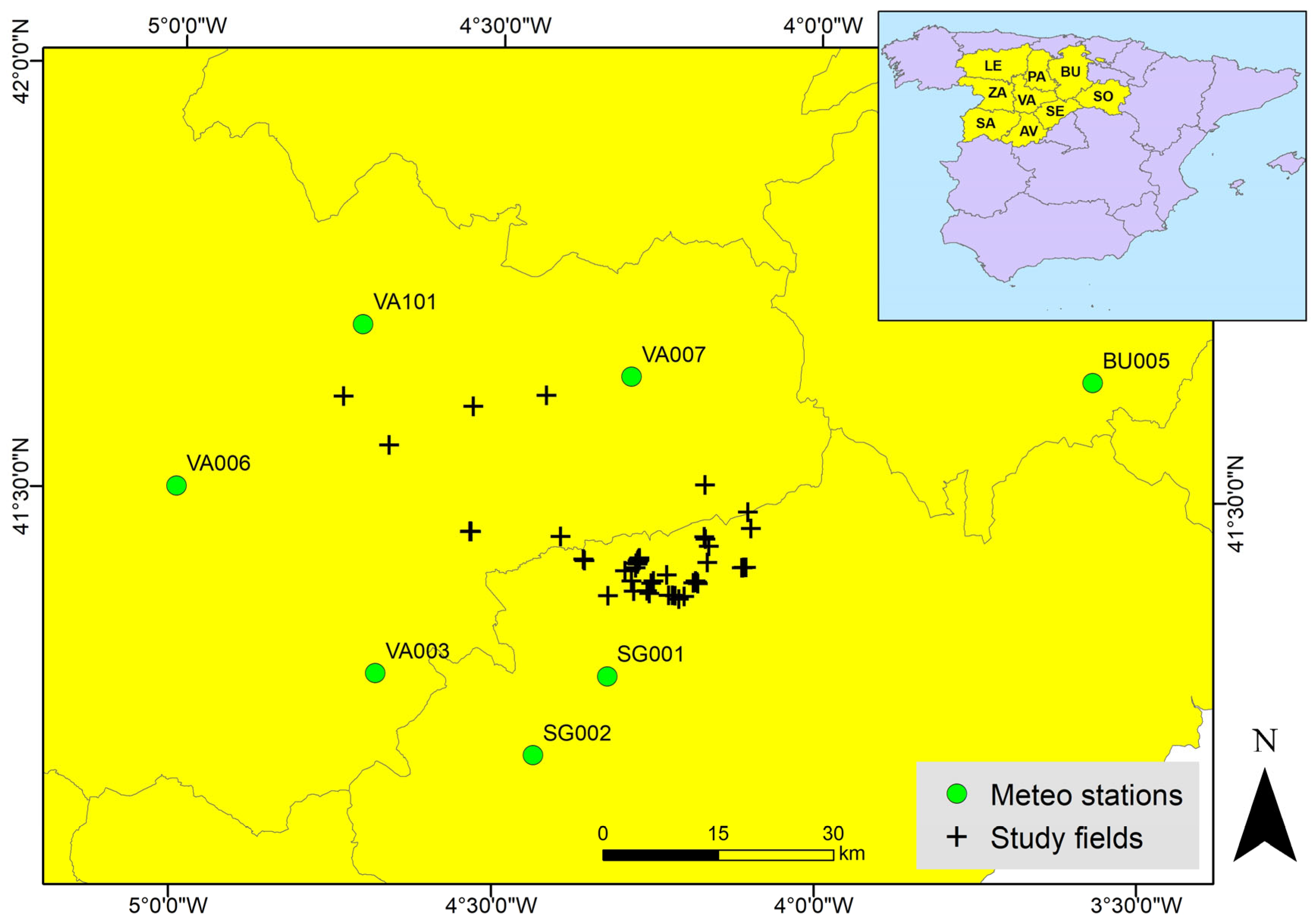
2.1. Study Area and In Situ Data

The study area is situated within the Castilla y León region of Spain, the country’s foremost potato-producing region, with an estimated 17,300 hectares dedicated to this crop [41]. Characterized by a Mediterranean climate with cool, dry summers and cold, rainy winters (Csb) [42], the region’s potato cultivation season typically spans from April to October. Variations in growing periods are influenced by factors such as potato variety (e.g., early, medium, or late maturity) and regional differences like climate and soil type.

In this study, potato fields are arranged in a ridge and furrow system and use sprinkler irrigation, which is managed by the farmers to ensure optimal water supply for the crops. The research encompasses eight distinct potato cultivars, each selected based on maturity classification for consumption purposes. This diversity allows the study to capture a wide range of growth timelines across similar weather conditions. Comprehensive ground-field data were collected from 50 fields over five years (2017–2021) with in situ periodic visits, conducted every 7–10 days, depending on the information provided by the potato growers, to monitor the crop development and collect data on phenological stages. Field areas ranged from 1.1 to 27.1 hectares, with an average size of 6.6 hectares (std = 5.5 ha). Field boundaries were obtained from the SIGPAC dataset [43] and validated through on-site supervision, where growers’ reported parcel IDs were verified in situ using GPS to confirm a match with the digital parcel border. An inner buffer of 20 m was applied to minimize edge effects and ensure that the extracted spectral signals originated from within the parcel boundaries.

For this study, four critical phenological stages were identified using the BBCH-scale with its 3-digit code: Emergence (009), where the first shoots become visible above the soil surface; Closure (309), when the plant canopy covers the ground between rows; Flowering (608), marked by the appearance of the first flowers; and Onset of Senescence (901), characterized by the beginning of leaf yellowing and decline in plant vigor. Each stage was visually confirmed when approximately 50% of plants in a field reached the target development phase. Due to the variability in the timing of field visits (every 7 to 10 days), a degree of uncertainty is inherent in the stage determination. Growing degree-day (GDD) calculations were performed for each phenological stage using the equation: GDD = (Tmax + Tmin)/2—Tbase, where Tmax and Tmin are the daily maximum and minimum temperatures, respectively, and Tbase is the base temperature, set here at 7 °C in line with [44]. Importantly, our GDD calculations commenced from each field’s documented planting date, providing a consistent starting point for our analysis. The term ‘Days After Planting’ (DAP) refers to the number of days elapsed since the planting date of the crop. In our study, we specifically examined the period from 0 DAP (the day of planting) to 199 DAP. This 200-day period was selected based on expert knowledge of the region’s agricultural practices and the growth cycles of the specific potato varieties under study. It represents a conservative timeframe that ensures the full growth cycle of the crop is captured, including all critical phenological stages up to and beyond the typical maturation point. By extending to 199 DAP, we aimed to mitigate the risk of prematurely ending our observation period and potentially missing late-season phenological events or variations in harvest timing due to unforeseen factors.

This considered periodization allowed for a standardized comparison across fields and years and was crucial for aligning satellite observation data with the observed phenological stages.

2.2. Satellite Data

2.2.1. Sentinel-1 (S1)

S1 imagery was acquired using the COPERNICUS/S1_GRD_FLOAT collection on the Google Earth Engine (GEE) platform. The S1 mission provides data from a dual-polarization C-band Synthetic Aperture Radar (SAR) instrument operating at 5.405 GHz (C band), with a nominal revisit time of 6 days. However, the revisit time was impacted by the S1B satellite failure, which occurred in December 2021, resulting in a complete dependence on S1A for continued data acquisition [45]. The data were acquired in the Interferometric Wide (IW) swath mode, offering a 250 km swath with a spatial resolution of 5 × 20 m. We utilized the Level-1 Ground Range Detected (GRD) product, which provides Synthetic Aperture Radar (SAR) images at a spatial resolution of 20 × 22 m and a pixel spacing of 10 × 10 m. The imagery was collected in both ascending and descending modes and included dual polarizations (VV and VH) from March 2017 to December 2021. During this period, our analysis utilized a total of 945 SAR images.

Preprocessing was conducted through a custom workflow within the GEE environment, based on the framework developed by [46] and supported by several key references, including [47,48,49,50]. This workflow included several essential steps to ensure the data were analysis-ready. Precise orbit files were applied to each image to achieve accurate geolocation. The images underwent radiometric calibration to sigma nought, facilitating consistent comparison across images acquired by the same sensor at different times. To mitigate speckle noise while preserving essential features such as edges and textures, the Refined Lee filter, with a kernel size of 5 × 5, was applied. This filter is renowned for its ability to maintain image quality by preserving linear features, point targets, and texture information [51,52,53]. Geometric distortions inherent in SAR data were addressed using the terrain flattening operator, with the USGS SRTMGL1_003 Digital Elevation Model (DEM) employed for topographic corrections [50,54]. Sigma nought backscatter values were subsequently converted from a linear to a logarithmic scale (dB). We then calculated the mean and standard deviation (std) of the backscatter values within each polygon.

To create a continuous daily time series, we applied an interpolation technique to the pre-processed S1 data. The interpolation method used was a smoothing spline function, as implemented in the smooth.spline function in R [55]. This uses a penalized likelihood approach to fit a smooth curve to the data. Smoothing spline functions have been successfully used in various studies for reconstructing time series, such as [56]. The smoothing parameter (spar) was set to 0.5, which was chosen based on visual inspection of the data to achieve a balance between capturing the underlying trends and minimizing overfitting. This approach enabled the estimation of daily values for each polarization (VH and VV), effectively filling gaps between acquisitions and reducing noise in the data.

We used a modified Z-score method to identify outliers, where points with residuals more than 1.64 times (corresponding to approximately the 90th percentile) the standard deviations away from the mean residual were considered outliers. This threshold was chosen to balance the need to remove noisy data points with the need to retain a sufficient number of data points for accurate spline fitting. This approach enabled us to derive daily values for each polarization (VH and VV), effectively filling gaps between acquisitions and reducing noise. An example of the time series data and the application of the quality assessment process is provided in the Supplementary Materials (Figures S1 and S2). The interpolated daily time series was then clipped to coincide with the crop’s growth cycle, spanning from 0 to 199 DAP. By focusing on this critical growth period, we ensured that our analysis captured the most relevant information on crop development.

2.2.2. Sentinel-2 (S2)

S2 imagery was acquired and processed using the COPERNICUS/S2_SR_HARMONIZED collection on the GEE platform. The dataset includes data from the S2A and S2B satellites, covering the period from March 2016 to the present, with a revisit time of approximately five days. The imagery is atmospherically corrected to Level-2A using the Sen2Cor algorithm and includes cloud masking to enhance data quality. The dataset includes 12 spectral bands: the Coastal aerosol band (B1) at 60 m resolution; Blue (B2), Green (B3), and Red (B4) bands at 10 m resolution; Red edge bands (B5 to B7) at 20 m resolution; the Near-Infrared (NIR) band (B8) at 10 m resolution and band (B8A) at 20 m resolution; the Water vapor band (B9) at 60 m resolution; and the Shortwave Infrared (SWIR) bands (B11 and B12) at 20 m resolution [57]. This collection also provides additional information through the Scene Classification Layer (SCL), generated using a combination of spatial and spectral analysis techniques, which helps to filter out unwanted features such as clouds, shadows, and other non-surface elements that may interfere with surface reflectance analysis. Further information about the nature of the additional classes can be found at the Earth Engine DATA catalog [58].

The processing involved filtering imagery from March 2017 to December 2021. Prior to any preprocessing, the dataset comprised 1239 images. Each polygon was buffered by 20 m inward to refine the analysis boundary, reducing spectral interference from neighboring parcels. For each field and acquisition date, we extracted pixel values and their frequencies. To enhance the accuracy of our analysis, we initially applied a cloud filtering process to the S2 data. For each acquisition date and polygon, we used the SCL to flag pixels as either reliable or unreliable. We retained pixels classified as Vegetation (class 4) and Bare Soils (class 5), while excluding pixels classified as clouds with medium probability (class 8), high probability (class 9), or thin cirrus clouds (class 10). However, we recognized that the SCL classification might not capture all cases of unreliable pixels (e.g., shadow). To further refine our dataset, we calculated pixel-level NDVI and further analyzed these values to identify potentially contaminated or noisy pixels, even those initially deemed reliable by the SCL. We then assessed each pixel’s NDVI using specific criteria to assign a high- or low-quality flag. Specifically, we calculated the weighted mean and standard deviation of NDVI values derived from histogram data for each parcel and each date of acquisition. Pixels were flagged as high quality if their NDVI values were within an 86.6% confidence interval (corresponding to 1.5 times the std from the weighted mean). Pixels outside this range were flagged as low quality or potential outliers. This refined dataset allowed us to create a look-up table that attributed a quality flag to each pixel, taking into account both its SCL classification and NDVI value. This table enabled us to apply the same quality assessment to the rest of the S2 bands, ensuring that our subsequent analysis was based on high-quality, reliable data.

Next, we used the quality-flagged data to create a continuous daily time series for each polygon and band using the weighted mean. We used smoothing splines, as performed for S1, to interpolate the reliable data points and generate a daily time series for each band. The spar value was chosen based on visual inspection to balance capturing underlying trends and minimizing overfitting. An example of the time series data and the application of the quality assessment process is provided in the Supplementary Materials (Figures S3 and S4). This approach filled the gaps between the original 5-day satellite overpass dates, producing a smoothed daily record that reduced noise. The resulting time series was then clipped to align with the crop’s growth period, defined as 0 to 199 days after planting (DAP).

The data processing and quality assessment steps outlined above enabled the calculation of various vegetation indices using daily time series data. These included the NDVI Equation (1), which has been widely used to derive phenological stages in various crops [59,60,61]. Additional indices, such as the Inverted Red-Edge Chlorophyll Index (IRECI2) Equation (2) and the biophysical Fraction of Absorbed Photosynthetically Active Radiation (fAPAR), were also computed to provide further insights into crop status and phenological development [62,63,64].

$$NDVI={\displaystyle \frac{(R842-R665)}{(R842+R665)}}$$

(1)

$$IRECI2={\displaystyle \frac{(R783-R665)}{(R740+R705)}}$$

(2)

where R842 nm corresponds to the reflectance value at band 8 (NIR), R783 to band 7, R740 to band 6, R705 to band 5, and R665 nm to band 4 (red).

Following the method proposed in [63,65,66], we calculated the fAPAR biophysical variable given its direct relation with the productivity of living vegetation [64]. We calculated fAPAR using two linear equations, referred to as the fAPAR_NDVI and fAPAR_SR models. The fAPAR_NDVI model relates fAPAR to NDVI, using minimum and maximum NDVI values corresponding to the 2nd and 98th percentiles of the NDVI frequency distribution. Similarly, the fAPAR_SR model relates fAPAR to the simple ratio (SR), which is a transformation of NDVI, and uses minimum and maximum SR values calculated from the NDVI values at the 2nd and 98th percentiles. We calculated fAPAR_SR and fAPAR_NDVI using these models and then computed the average fAPAR as the mean of these two values. For further details, please refer to the aforementioned works.

2.3. Meteorological Data

Meteorological conditions play a fundamental role in the timing of phenological changes. Although we only focus on the signal registered by the onboard sensors on satellite platforms, climate data can be very informative in interpreting the model fitting and results. For instance, radar backscatter is highly affected by water in the soil and canopy [67,68]. To remove these effects, authors whose study fields are under rain-fed regimes simply flag/drop those days in which there are rainy episodes. This approach could not be used in our study, given the circumstances of the fields (neither rain-fed nor having irrigation dates). In addition, the extremely variable rainfall between locations, especially during summer when most of the convective storms occur in the area, makes the use of rain gauge measurements located on close-by locations very inaccurate.

We retrieved climate data from the network of ground-based meteorological stations [69] and the closest selected stations (“BU05”, “SG01”, “SG02”, “VA03”, “VA06”, “VA07”, “VA10”) to better interpret climate variability in the study period (Figure 1). They are equipped with Campbell Scientific pluviometers (ARG100) to measure precipitation, and Rotronic (HC2 S3) sensors for air temperature. Temperature data was used for calculating GDDs, which are typically used for assessing crop development stages. This calculation allows us to cross-compare our in situ measurements with other studies in different locations, providing a benchmark to assess whether our fields are representative of broader regional or global trends. Meteorological data is provided as Supplementary Materials (Figures S5–S11).

3. Methods

3.1. Assumptions

According to the current state of the art for other crops [27,30,60], the expected behavior of signal reflectance and backscatter is to increase as the first shoots and leaves above the ground emerge. Some fluctuations in the curves are expected during the first one to two months due to the influence of weed, soil moisture/roughness in the spectral and backscatter response. The closure is reached when plant leaves from adjacent rows meet, soil is covered, and the crop is close to the maximum above-ground development. At this stage, the slope of VIs curves typically approaches 0 (plateau) with a slight increase (or decrease) in the following days to weeks, expecting similar behavior in SAR data as the volumetric scattering associated with plant development becomes constant and the soil influence is removed. SAR data, particularly in C-band imagery, has been shown to effectively capture temporal changes in crop characteristics like the heading phase in wheat [70] or biomass [26]. Based on this, we hypothesize that SAR backscatter response could potentially be used to detect potato flowering. We are unaware of any instances where optical data has been utilized for potato flowering detection; therefore, we did not attempt to identify this phase using optical data, lacking a clear expectation of the associated patterns in the vegetation indices considered. The onset of senescence is characterized by the beginning of leaf yellowing, and a gradual decrease in photochemical efficiency, Vegetation Water Content, and plant height. These crop changes imply a steady decrease in VIs values and an increase in the variability of SAR backscatter, given the higher sensitivity to the underlying soil layer [27]. Before harvest, mechanical/physical haulming (destruction of the potato haulm) ensures a more homogenous tuber maturity at the field level, stops bulking to meet marketable requirements, and improves and speeds skin-set and stolon separation [71]. In the fields being investigated, high-haulm varieties underwent chemical or mechanical haulming, typically occurring 10 to 30 days before harvest. However, in certain cases, no haulming was conducted, and the plants naturally senesced. The haulming process resulted in a sudden decline in VIs and volumetric scattering, thereby amplifying the influence of soil in remote sensing images. Figure 2 illustrates the primary stages identified in this process.

3.2. Phenology Detection

This study employed a phenology detection approach that involved analyzing pre-processed time series data using a curve-specific time-based algorithm, tailored to capture distinct characteristics of the crop using SAR (e.g., canopy structure) and optical data (e.g., photosynthetic activity) (Figure 3). Although similar curve-based approaches have been applied to other crops and indices in previous studies, such as those by [27,60], our method is uniquely designed for potato crops, considering the specific growth patterns and environmental interactions captured by SAR and optical data. The approach relies on fitting splines to the data and computing their first and second derivatives to interpret the slope and curvature of the curves at each point, allowing for the identification of key phenological stages. This approach relies on a set of assumptions that are tailored to the characteristics of SAR and optical data, based on the expected patterns and trends in the time series. The thresholds and algorithmic rules were determined through a combination of domain knowledge, iterative refinement, and an understanding of the expected physical interactions between the potato crop canopy and the SAR and optical signals.

To further enhance the accuracy of our phenology detection approach, we integrated the date predictions from S2-NDVI and S1-VH by calculating the average of the estimated dates for each phenological stage and field. This integration aimed to capitalize on the complementary strengths of both data types, combining NDVI’s sensitivity to vegetation health with VH backscatter’s responsiveness to crop structure or leaf water content. By merging these indices, we expected to mitigate potential biases and obtain a more comprehensive and robust assessment of phenological stages, leveraging the unique advantages of each data type to improve the overall predictive performance.

To detect emergence, we consider the point when 50% of the field has plants out. For optical data (S2), the signal is sensitive to early plant growth, with initial increases observed as the first plants emerge. As the field continues to green up, the curve is expected to shift from a stable low signal to a rapid increase, and we detect emergence by finding the first point where the slope exceeds the 75th percentile of positive slopes, starting from DAP 0. For SAR data (S1), emergence is marked by a change in the curve where, after an initial period influenced by bare soil moisture, the first derivative becomes positive and is sustained for 6 days or longer (S1 revisit time). The difference in approaches is due to the distinct characteristics of each sensor: optical sensors (S2) may detect initial plant growth stages earlier, while SAR (S1) signals may be masked by soil moisture at early stages, requiring a more robust trend detection.

In contrast, the closure phase is characterized by significant signal reduction in soil and growth stabilization, marked by a concave down (increasing) curve. We identify the closure phase as the point where the first derivative is positive, and the second derivative reaches its minimum value among all instances with a positive first derivative, indicating a change in the curve’s slope. This rule applies to both SAR and optical data.

The flowering phase, which is solely derived from SAR data, is characterized by a concave-up curve. We assume that the presence of inflorescence and flowers will lead to an increase in backscatter, causing a reduction in the signal received by the SAR sensor. As the flowers begin to wilt, the plant structure changes again, resulting in an increase in the SAR signal. This phase is identified at the local minimum where the first derivative is near zero and the second derivative is positive.

The senescence implies the onset of vegetation decline and is characterized by a concave downward (decreasing) curve. For both optical and SAR data, we assume that the senescence phase begins when the curve starts to decrease, marked by a negative first derivative and the lowest second derivative from the flowering point. However, the curve behavior differs between the two data types. For optical data, the curve typically exhibits a single peak, followed by a continuous decrease. In contrast, SAR data may exhibit multiple peaks after flowering, due to the complex interaction between the radar signal and the canopy structure. To address this, we identify the first peak after flowering in SAR data, and then select the point where the curve starts to decrease, marked by a negative first derivative and the lowest second derivative.

Finally, the harvest time is established using different approaches for optical and SAR data, with the analysis confined to the period between the senescence phase and the end of the time series (DAP 199). For optical, the harvest is detected by finding the point where the decrease in the signal relaxes or flattens between the senescence phase and the end of the time series. This is performed by identifying the point where the first derivative is negative and the second derivative is at its maximum value. In contrast, the harvest point for SAR data is detected using a more complex approach, as SAR signals exhibit greater variability due to soil and other factors, especially when biomass decreases and following harvest. As the crop senesces, the SAR signal becomes more sensitive to soil moisture and roughness, causing variability with multiple peaks and valleys. To minimize this effect, the algorithm requires the first derivative to remain negative for at least 14 days after senescence onset, a threshold based on the fastest possible senescence scenario with chemical desiccation [72]. The algorithm considers peaks and valleys or softer slopes after the senescence onset. It identifies the point before a valley where the first derivative is negative and the second derivative is at its maximum, or the point where the slope flattens (first derivative less negative, second derivative near zero), focusing on the first valley if multiple are present. For a visual representation of how these assumptions and descriptions are applied to the curves, please refer to the Supplementary Materials (Figure S12), which provide an exemplary curve for a single field planted in 2021, with the corresponding points selected for each phenological stage using S1 and S2 data.

The retrieved DAP for each field and phase were validated by comparing them with in situ measurements. The dates of the detected phenological changes were compared to those collected in situ. We used the Root Mean Squared Error (RMSE) and the coefficient of determination (R²) to assess the accuracy of the method per stage, as these metrics are commonly used in similar studies [73,74].

To ensure the generalizability of our findings beyond our local study area, we compared our determined phenological stage ranges with the existing literature on potato crop phenology. We reviewed relevant studies conducted in diverse geographic regions and under different experimental conditions to assess whether our identified AGDD threshold ranges align with previously reported observations. Additionally, we established a baseline model using the average GDD values from the literature (including our in situ data) to estimate the days after planting (DAP) for each phase and field. This allowed us to evaluate the performance of our phenology detection algorithm against a simple, literature-based approach and assess its accuracy by comparing the estimated DAP values to the actual DAP values from in situ observations.

4. Results

4.1. Description of In Situ Observations

Our analysis from 50 fields over five years reveals that emergence typically occurs around 37 DAP on average, with a std of 8 days (Table S1). This date is controlled by several factors such as climate conditions, soil type, variety, or the timing of seeds being taken out from refrigeration before planting. The mean dates for closure (70 DAP) and flowering (77 DAP) were relatively close in time, also linked to agronomical and climatic conditions. As anticipated, the onset of senescence (99 DAP) and harvest time (163 DAP) exhibited greater variability around the mean, reflecting the diverse maturity profiles of our potato varieties across the full maturity spectrum. Our observed phenological dates are consistent with the 90% confidence interval (CI) ranges reported in other studies, as shown in Figure S13 and Table S2. This suggests that the patterns observed in the studied fields are consistent with the general trends of potato crop development reported in the literature, which is notable given that these fields, although localized, appear to be representative of broader regional and global patterns, despite variations in climate, soil type, agronomic practices, and potato varieties.

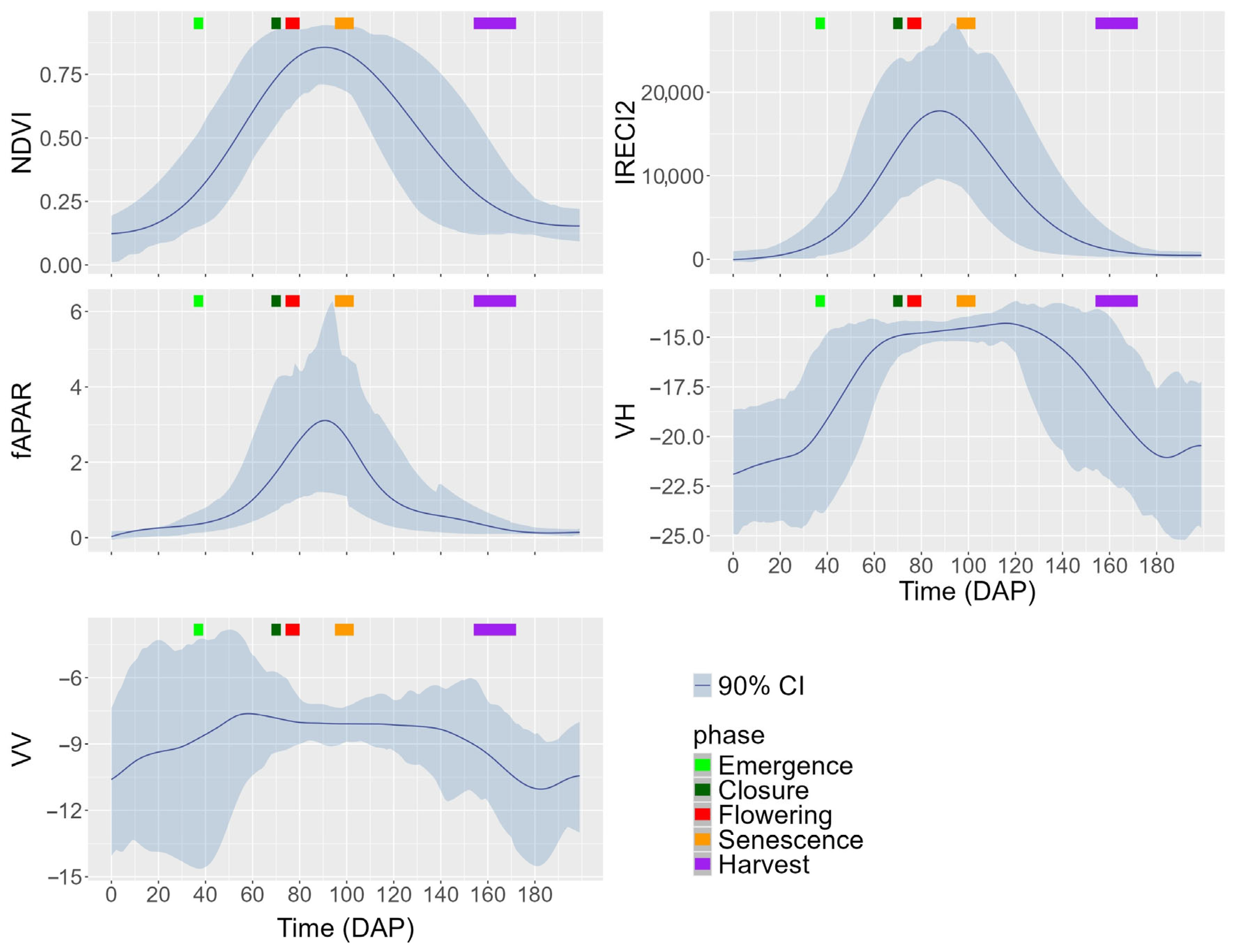
4.2. Description of Curves and Their Variability Across DAPs

For the three VIs from S2—NDVI, IRECI2, and fAPAR—the mean curves exhibit a bell-shaped distribution, with NDVI showing the broadest curve, IRECI2 being narrower, and fAPAR being the flattest. All three indices peak between 80 and 100 DAP. The variability, represented as the 90% CI (5th–95th percentiles), indicates that NDVI has greater variability between 110 and 170 DAP. IRECI’s variability is more consistent throughout the crop’s lifespan, from 50 to 150 DAP, while fAPAR shows increased variability from 60 to 120 DAP, peaking at 80–100 DAP.

The mean VH time series curve, unlike the bell-shaped optical indices, features an initial slow increase (0–30 DAP), followed by a rapid ascent (30–60 DAP), a sustained plateau (60–120 DAP), and a final decrease with some perturbations at the end (Figure 4). Variability in VH is most pronounced at the beginning and end of the crop cycle, specifically from 0 to 40 DAP and 140 to 199 DAP. The VV time series curve shows a similar trend, with the mean increasing until 60 DAP, forming a plateau that stabilizes until around 140 DAP, and then decreasing and stabilizing. Variability in VV is greatest from 0 to 60 DAP and increases again from 140 DAP onwards. The variability observed in both VH and VV may be influenced by several factors. During the early stages of the crop cycle, soil conditions play a significant role, particularly when the soil is bare or only partially covered. In the study area, sowing occurs from April to mid-May, which are typically wet months (Figures S2–S8), leading to high variability in VH and VV backscatter. As the crop progresses into the senescence stage, changes in canopy structure and soil water content, influenced by factors such as irrigation and variations in above-ground biomass, further contribute to the observed variability. Additionally, differences in potato maturity times and agronomic practices, like haulming and pest management, lead to greater variability across fields.

4.3. Performance of the Detection Algorithm per Phase and Variable

The performance of the phenology detection algorithm varied, resulting in a range of RMSE values (

Table 1. Root Mean Squared Error (RMSE) per variable and phase measured in days.

RMSE (Days)	Emergence	Closure	Flowering	Onset Senescence	Harvest
NDVI	12	14	-	17	29
IRECI2	13	19	-	19	44
fAPAR	13	22	-	17	52
VH	15	19	22	33	29
VV	15	24	23	30	28
NDVI_VH	12	15	22	19	23
Baseline	20	11	11	26	41

). For the emergence phase, the optical indices (NDVI, IRECI2, and fAPAR) and the combined S1–S2 method (NDVI_VH) exhibit relatively low RMSE values, ranging from 12 to 13 days. In contrast, the SAR indices (VH and VV) have slightly higher RMSE values for 15 days. Predictions for the optical indices and the combined S1–S2 method are generally well-aligned with the actual emergence dates due to their sensitivity to changes in vegetation greenness and canopy development, without consistently predicting earlier or later than the actual dates (Figure 5). However, SAR indices tend to predict emergence slightly earlier than the actual dates, indicating a mild underestimation. The closure phase ranged from 14 (NDVI) to 24 (VV) days. Scatter plots reveal no bias for NDVI, VH, and NDVI_VH, while IRECI2 and fAPAR overestimate and VV underestimates closure dates.

Flowering detection for VH and VV polarizations had RMSE values of 22–23 days. VV polarization had slightly higher variability than VH, with no clear bias. This phase was optimized for SAR data, which excels at capturing surface roughness changes, and no optical estimates are available. NDVI_VH used only VH values, and phase proximity caused points to mix across fields with different timing. Senescence RMSE values ranged from 17 to 33 days, with optical indices (NDVI, IRECI2, fAPAR) generally underestimating onset, while SAR polarizations (VH, VV) showed overestimation (VH) and higher variability (VV). The combined NDVI_VH balanced the underestimation of optical indices and the overestimation of VH, showing better alignment with actual values. Harvest RMSE values ranged from 23 to 52 days, with NDVI_VH performing the best, while IRECI2 and fAPAR underestimated, and SAR indices overestimated harvest dates. Optical signals are hindered by rain and cloud cover during the harvest season (October–November), whereas SAR signals are impacted by soil moisture. Furthermore, harvest timing is also influenced by external factors such as farmer convenience and market conditions, which can lead to discrepancies between predicted and actual dates.

The combined NDVI_VH highlights the benefits of integrating S1 and S2 data, leveraging their complementary characteristics to achieve less biased estimates across emergence, onset of senescence, and harvest. For instance, during emergence, NDVI_VH combines NDVI’s sensitivity to vegetation greenness with VH’s stability, while in senescence, it balances NDVI’s underestimation with VH’s overestimation. Similarly, during harvest, NDVI_VH leverages VH’s responsiveness to crop moisture and NDVI’s sensitivity to dry vegetation. This integration overcomes individual index limitations, resulting in a more comprehensive and accurate assessment of crop phenology. While it may not always outperform other indices in every phase, its stable performance across phases demonstrates the value of combining these indices.

Overall index performance was evaluated by aggregating data points from all phases and analyzing their prediction accuracy (Figure 5). NDVI exhibited an RMSE of 17 days and an R² of 0.83, with no clear under- or over-estimation, although higher variability was observed at later phases. In contrast, IRECI2 and fAPAR showed RMSE of 23 and 26 days, and R² values of 0.72 and 0.64, respectively, with a tendency to overestimate emergence and closure, and underestimate senescence and harvest. The SAR-based indices, VH and VV, had RMSE of 24 days and R² of 0.78 and 0.76, respectively, characterized by higher variability around the one-to-one line, particularly at later phases. The integrated approach, NDVI_VH, had an RMSE of 18 days and an R² of 0.80, with less variability across the phases, indicating a more consistent performance.

The accuracy of the phenology detection algorithm is compared to a baseline model based on GDDs reported in the literature (Figure 6). Our curve-based method performs better than the baseline model for emergence (all indices), senescence (NDVI, IRECI2, fAPAR, and NDVI_VH), and harvest (most indices). In contrast, the baseline performance is better for closure and flowering, although it is worth noting that the literature-based estimates for these phases are limited. This is particularly true for closure, where the baseline model is based solely on our in situ data (see Table S2), which is specific to the environmental and agronomic characteristics of our study area and, therefore, may not be representative of the broader spatial variability and regional patterns observed in other phases. Overall, the superior performance of our curve-based method can be attributed to its ability to leverage spatial observations from satellite data, providing a more accurate representation of crop phenology. In contrast, the GDD baseline method relies on a more parametric approach, which may not fully capture the complexities of crop growth and development, such as variations in crop variety, soil type, and local environmental conditions.

5. Discussion

This study provides a comprehensive analysis of phenological stage detection in potatoes, combining optical and SAR data for agricultural monitoring, which is essential for large-scale management and historical analysis of crop yield [75]. In situ observations are limited by the need for frequent and often time-consuming field visits, making remote sensing a more efficient, cost-effective, and practical alternative for data collection. We used spline fitting, a method well-suited for post-season analysis, to compare and combine S1 and S2-based indices. While it has limitations for real-time monitoring [76], including time-delay [77] and sensitivity to missing data [78], it enabled a comprehensive evaluation of their performance in detecting phenological stages, as documented in studies with similar purposes [79,80,81]. Alternative methods, such as sigmoid functions, can be used for within-season analysis [76,82], but their accuracy may be compromised due to sensitive and uncertain parameters. This limitation is consistent with previous studies, which have shown that the sigmoid model’s curve parameters are uncertain and sensitive, particularly when observational data are limited [83,84,85].

The differences in sensitivity between optical and radar data can have significant implications for crop monitoring. Optical data, which are sensitive to changes in vegetation reflectance, can provide detailed information on crop growth and development, as well as biophysical and biochemical parameters [86]. In contrast, radar data, which are particularly sensitive to variations in surface roughness, offer a more stable and consistent signal across different parcels. While they may be less responsive to certain changes in crop growth or biochemical parameters, radar data excel in assessing soil moisture, surface roughness, and crop structure [87]. Some studies demonstrate how radar data can complement optical data, enhancing overall insights into crop monitoring [88].

Our results show that S2-based indices better captured emergence, closure, and onset of senescence, whereas SAR indices were more capable of detecting flowering and harvest timing. The use of NDVI for phase detection has been widely reported in the literature for other crops [89,90,91], and we also show its capacity for potatoes, while showing weakness in detecting harvest dates since human, market, and environmental circumstances play a major role. Despite the well-known issue of saturation in the red band [92], which can limit the detection of changes in high-coverage vegetation at their peak biomass, NDVI still emerged as the best index for detecting the onset of senescence. IRECI2 and fAPAR had generally good detection of emergence but systematically overestimated closure and underestimated senescence. In general, crop structural changes lag behind changes in vegetation pigment [93,94]; hence, using SAR and optical data together may enhance the accuracy and dependability of crop phenology detection. SAR-based indices presented a slight underestimation of emergence and overestimation in detecting harvest, with similar overall performances. The novel NDVI_VH approach performed well in phases where NDVI was strong, such as emergence, closure, and onset of senescence, and it was also effective in phases where NDVI had limitations, including flowering, which was not estimable with NDVI, and harvest, where VH contributed to enhanced accuracy. By combining NDVI and VH, we created a more robust method that leverages the strengths of both, resulting in a more consistent and reliable representation of crop phenology across different phases. To the best of our knowledge, this is the first study that used S1 alone or combined with S2 data to identify phenological status in potatoes.

The RMSE values reported in this study (ranging from 12 to 52 days) provide a quantitative assessment of the accuracy of each index and phase (including harvest). However, these values must be interpreted in the context of several limitations. Data availability and quality can impact the accuracy of our detection algorithm, due to factors like satellite revisit frequency, cloud cover, and soil conditions (including soil moisture and water-on-canopy conditions). Cloud cover is a significant issue, particularly from March to mid-May and mid-September onwards, affecting S2 data for the emergence and harvest seasons. Soil effects and weed impact also affect S2-based data, while SAR data is affected by irrigation or rainfall. Additionally, the SAR data’s time resolution has increased to 10 days since the S1B failure, potentially impacting accuracy. Some uncertainty is also expected in in situ data due to measurement bias in phenological detection.

Consistent with previous studies [76,95,96,97,98], we confirm the potential of optical and SAR remotely sensed data to detect phenological stages in potato crops. However, a common challenge in this field is the extrapolation of results from small-scale, in situ measurements to larger areas, which can limit the generalizability of these findings. Our results show that crop life cycles and phenological phases align with those reported in other studies across different regions, with varying soils, climates, varieties, and agricultural practices. We used a 50% threshold to define key growth stages, consistent with other researchers (e.g., [99]), and our comparison with independent studies (Table S1) reveals similar phase ranges despite varying environmental and agricultural conditions. This suggests that our algorithm captures underlying patterns of crop development, making it applicable to other potato fields with different characteristics. Additionally, Table S3 provides context by comparing our study with phenology research in other crops [80,100,101,102], showing where our work stands within the current state of the art.

While our study focuses on post-season analysis, these results highlight the potential for operational use in near-real-time for managing farming practices (e.g., irrigation scheduling, fertilizer management, and harvesting operations) [103,104,105] and better crop yield estimations [100]. However, to implement these methods in real-time, challenges such as the need for post-time data to detect inflection points and limitations due to satellite revisit schedules and cloud cover must be addressed. Continued advancements in satellite technology and data processing will be key to overcoming these obstacles and enhancing the practical applicability of our methods across different agricultural contexts.

6. Conclusions

Our results show the effectiveness of individual and integration of S1 and S2 time series data for identifying key phenological stages in potato crops at the field scale, thereby overcoming the limitations of individual sensors. The methodology developed in this study, which leverages 5 years of in situ data from the Castilla y Leon region (Spain) to compare the capacity of optical and SAR sensors, provides a framework for phenological stage detection, at this stage, for post-season analysis. The findings of this study have important implications for agricultural management and global food security, as the proposed methodology can provide valuable insights into crop development and phenology, ultimately refining crop growth models, improving harvest forecasting, and informing planning of agricultural practices that can help mitigate the impacts of climate change and contribute to more resilient agricultural systems.

Future studies could explore the use of newer satellite sensors, additional vegetation indices, and integration with other data sources to further improve the accuracy and applicability of phenology detection models. This could also involve collecting more in situ data across different regions and climates to validate and refine these models.

References

1. Fanzo, J.; Davis, C.; McLaren, R.; Choufani, J. The Effect of Climate Change across Food Systems: Implications for Nutrition Outcomes. Glob. Food Secur. 2018, 18, 12–19. [Google Scholar] [CrossRef]
2. Lobell, D.B.; Burke, M.B.; Tebaldi, C.; Mastrandrea, M.D.; Falcon, W.P.; Naylor, R.L. Prioritizing Climate Change Adaptation Needs for Food Security in 2030. Science 2008, 319, 607–610. [Google Scholar] [CrossRef] [PubMed]
3. Myers, S.S.; Smith, M.R.; Guth, S.; Golden, C.D.; Vaitla, B.; Mueller, N.D.; Dangour, A.D.; Huybers, P. Climate Change and Global Food Systems: Potential Impacts on Food Security and Undernutrition. Annu. Rev. Public Health 2017, 38, 259–277. [Google Scholar] [CrossRef] [PubMed]
4. Vermeulen, S.J.; Campbell, B.M.; Ingram, J.S.I. Climate Change and Food Systems. Annu. Rev. Environ. Resour. 2012, 37, 195–222. [Google Scholar] [CrossRef]
5. Hall, C.; Dawson, T.P.; Macdiarmid, J.I.; Matthews, R.B.; Smith, P. The Impact of Population Growth and Climate Change on Food Security in Africa: Looking Ahead to 2050. Int. J. Agric. Sustain. 2017, 15, 124–135. [Google Scholar] [CrossRef]
6. IPCC. Climate Change and Land; IPCC: Geneva, Switzerland, 2019. [Google Scholar]
7. Kundzewicz, Z.W.; Mata, L.J.; Arnell, N.W.; Döll, P.; Jimenez, B.; Miller, K.; Oki, T.; Şen, Z.; Shiklomanov, I. The Implications of Projected Climate Change for Freshwater Resources and Their Management. Hydrol. Sci. J. 2008, 53, 3–10. [Google Scholar] [CrossRef]
8. IPCC. AR5 Climate Change 2013: The Physical Science Basis; Cambridge University Press: Cambridge, UK, 2013. [Google Scholar]
9. EPA. NOAA Climate Change Indicators-Us and Global; EPA: Washington, DC, USA, 2016. [Google Scholar]
10. Webber, H.; Gaiser, T.; Ewert, F. What Role Can Crop Models Play in Supporting Climate Change Adaptation Decisions to Enhance Food Security in Sub-Saharan Africa? Agric. Syst. 2014, 127, 161–177. [Google Scholar] [CrossRef]
11. Gonzalez Piqueras, J.; Jara, J.; López, H.; Villodre, J.; Hernández, D.; Calera, A.; López-Urrea, R.; Sánchez, J.M. Determining Crop Phenology for Different Varieties of Barley and Wheat on Intensive Plots Using Proximal Remote Sensing. In Proceedings of the Remote Sensing for Agriculture, Ecosystems, and Hydrology XXI, Strasbourg, France, 21 October 2019; Neale, C.M., Maltese, A., Eds.; SPIE: Bellingham, WA, USA, 2019; p. 19. [Google Scholar]
12. Ruml, M.; Vulic, T. Importance of Phenological Observations and Predictions in Agriculture. J. Agric. Sci. Belgrade 2005, 50, 217–225. [Google Scholar] [CrossRef]
13. Aslam, M.A.; Ahmed, M.; Stöckle, C.O.; Higgins, S.S.; Hassan, F.U.; Hayat, R. Can Growing Degree Days and Photoperiod Predict Spring Wheat Phenology? Front. Environ. Sci. 2017, 5, 57. [Google Scholar] [CrossRef]
14. Setiyono, T.D.; Weiss, A.; Specht, J.; Bastidas, A.M.; Cassman, K.G.; Dobermann, A. Understanding and Modeling the Effect of Temperature and Daylength on Soybean Phenology under High-Yield Conditions. Field Crops Res. 2007, 100, 257–271. [Google Scholar] [CrossRef]
15. Shaykewich, C.F.; Bullock, P.R. Modeling Soybean Phenology. In Agronomy Monographs; Hatfield, J.L., Sivakumar, M.V.K., Prueger, J.H., Eds.; American Society of Agronomy, Crop Science Society of America, and Soil Science Society of America, Inc.: Madison, WI, USA, 2018; pp. 279–302. ISBN 978-0-89118-358-7. [Google Scholar]
16. Soltani, A.; Hammer, G.L.; Torabi, B.; Robertson, M.J.; Zeinali, E. Modeling Chickpea Growth and Development: Phenological Development. Field Crops Res. 2006, 99, 1–13. [Google Scholar] [CrossRef]
17. Hufkens, K.; Melaas, E.K.; Mann, M.L.; Foster, T.; Ceballos, F.; Robles, M.; Kramer, B. Monitoring Crop Phenology Using a Smartphone Based Near-Surface Remote Sensing Approach. Agric. For. Meteorol. 2019, 265, 327–337. [Google Scholar] [CrossRef]
18. ESA. New Satellite for Unprecedented Earth Monitoring; ESA: Paris, France, 2015. [Google Scholar]
19. Zheng, Y.; Wu, B.; Zhang, M.; Zeng, H. Crop Phenology Detection Using High Spatio-Temporal Resolution Data Fused from SPOT5 and MODIS Products. Sensors 2016, 16, 2099. [Google Scholar] [CrossRef] [PubMed]
20. You, X.; Meng, J.; Zhang, M.; Dong, T. Remote Sensing Based Detection of Crop Phenology for Agricultural Zones in China Using a New Threshold Method. Remote Sens. 2013, 5, 3190–3211. [Google Scholar] [CrossRef]
21. USGS NDVI. The Foundation for Remote Sensing Phenology; USGS: Sunrise Valley Drive Reston, VA, USA, 2020. [Google Scholar]
22. Joshi, N.; Baumann, M.; Ehammer, A.; Fensholt, R.; Grogan, K.; Hostert, P.; Jepsen, M.; Kuemmerle, T.; Meyfroidt, P.; Mitchard, E.; et al. A Review of the Application of Optical and Radar Remote Sensing Data Fusion to Land Use Mapping and Monitoring. Remote Sens. 2016, 8, 70. [Google Scholar] [CrossRef]
23. Della Vecchia, A.; Ferrazzoli, P.; Guerriero, L.; Ninivaggi, L.; Strozzi, T.; Wegmuller, U. Observing and Modeling Multifrequency Scattering of Maize During the Whole Growth Cycle. IEEE Trans. Geosci. Remote Sens. 2008, 46, 3709–3718. [Google Scholar] [CrossRef]
24. Inoue, Y.; Sakaiya, E.; Wang, C. Capability of C-Band Backscattering Coefficients from High-Resolution Satellite SAR Sensors to Assess Biophysical Variables in Paddy Rice. Remote Sens. Environ. 2014, 140, 257–266. [Google Scholar] [CrossRef]
25. Vreugdenhil, M.; Wagner, W.; Bauer-Marschallinger, B.; Pfeil, I.; Teubner, I.; Rüdiger, C.; Strauss, P. Sensitivity of Sentinel-1 Backscatter to Vegetation Dynamics: An Austrian Case Study. Remote Sens. 2018, 10, 1396. [Google Scholar] [CrossRef]
26. Schlund, M.; Erasmi, S. Sentinel-1 Time Series Data for Monitoring the Phenology of Winter Wheat. Remote Sens. Environ. 2020, 246, 111814. [Google Scholar] [CrossRef]
27. Khabbazan, S.; Vermunt, P.; Steele-Dunne, S.; Ratering Arntz, L.; Marinetti, C.; Van Der Valk, D.; Iannini, L.; Molijn, R.; Westerdijk, K.; Van Der Sande, C. Crop Monitoring Using Sentinel-1 Data: A Case Study from The Netherlands. Remote Sens. 2019, 11, 1887. [Google Scholar] [CrossRef]
28. Mercier, A.; Betbeder, J.; Baudry, J.; Le Roux, V.; Spicher, F.; Lacoux, J.; Roger, D.; Hubert-Moy, L. Evaluation of Sentinel-1 & 2 Time Series for Predicting Wheat and Rapeseed Phenological Stages. ISPRS J. Photogramm. Remote Sens. 2020, 163, 231–256. [Google Scholar] [CrossRef]
29. Nasrallah, A.; Baghdadi, N.; El Hajj, M.; Darwish, T.; Belhouchette, H.; Faour, G.; Darwich, S.; Mhawej, M. Sentinel-1 Data for Winter Wheat Phenology Monitoring and Mapping. Remote Sens. 2019, 11, 2228. [Google Scholar] [CrossRef]
30. Song, Y.; Wang, J. Mapping Winter Wheat Planting Area and Monitoring Its Phenology Using Sentinel-1 Backscatter Time Series. Remote Sens. 2019, 11, 449. [Google Scholar] [CrossRef]
31. Stendardi, L.; Karlsen, S.R.; Niedrist, G.; Gerdol, R.; Zebisch, M.; Rossi, M.; Notarnicola, C. Exploiting Time Series of Sentinel-1 and Sentinel-2 Imagery to Detect Meadow Phenology in Mountain Regions. Remote Sens. 2019, 11, 542. [Google Scholar] [CrossRef]
32. Veloso, A.; Mermoz, S.; Bouvet, A.; Le Toan, T.; Planells, M.; Dejoux, J.-F.; Ceschia, E. Understanding the Temporal Behavior of Crops Using Sentinel-1 and Sentinel-2-like Data for Agricultural Applications. Remote Sens. Environ. 2017, 199, 415–426. [Google Scholar] [CrossRef]
33. FAO. Promotion of Underutilized Indigenous Food Resources for Food Security and Nutrition in Asia and the Pacific; FAO: Rome, Italy, 2014. [Google Scholar]
34. Wijesinha-Bettoni, R.; Mouillé, B. The Contribution of Potatoes to Global Food Security, Nutrition and Healthy Diets. Am. J. Potato Res. 2019, 96, 139–149. [Google Scholar] [CrossRef]
35. Hack, H.; Gall, H.; Klemke, T.; Klose, R.; Meier, U.; Stauss, R.; Witzenberger, A. Phänologische Entwicklungsstadien der Kartoffel (Solanum tuberosum L.). Codierung und Beschreibung nach der erweiterten BBCH-Skala mit Abbildungen. Das Nachrichtenblatt des Deutschen Pflanzenschutzdienstes 1993, 45, 11–19. [Google Scholar]
36. Aien, A.; Chaturvedi, A.K.; Bahuguna, R.N.; Pal, M. Phenological Sensitivity to High Temperature Stress Determines Dry Matter Partitioning and Yield in Potato. Indian J. Plant Physiol. 2017, 22, 63–69. [Google Scholar] [CrossRef]
37. Rykaczewska, K. The Effect of High Temperature Occurring in Subsequent Stages of Plant Development on Potato Yield and Tuber Physiological Defects. Am. J. Potato Res. 2015, 92, 339–349. [Google Scholar] [CrossRef]
38. Arana, C.; Orlando, R.; Laercio, Z.; Claudio, L. Potato early blight epidemics and comparison of methods to determine its initial symptoms in a potato field. Rev. Fac. Nac. Agron. 2007, 60, 3877–3890. [Google Scholar]
39. Gent, D.H.; Schwartz, H.F. Validation of Potato Early Blight Disease Forecast Models for Colorado Using Various Sources of Meteorological Data. Plant Dis. 2003, 87, 78–84. [Google Scholar] [CrossRef] [PubMed]
40. Hoelle, J.; Asch, F.; Khan, A.; Bonierbale, M. Phenology-Adjusted Stress Severity Index to Assess Genotypic Responses to Terminal Drought in Field Grown Potato. Agronomy 2020, 10, 1298. [Google Scholar] [CrossRef]
41. JCyL. Patata de Siembra; Junta de Castilla y Leon: Valladolid, Spain, 2021. [Google Scholar]
42. Kottek, M.; Grieser, J.; Beck, C.; Rudolf, B.; Rubel, F. World Map of the Köppen-Geiger Climate Classification Updated. Meteorol. Z. 2006, 15, 259–263. [Google Scholar] [CrossRef]
43. MAPA. Sigpac; MAPA: Ankara, Turkey, 2020. [Google Scholar]
44. Sands, P.J.; Hackett, C.; Nix, H.A. A Model of the Development and Bulking of Potatoes (Solanum tuberosum L.) I. Derivation from Well-Managed Field Crops. Field Crops Res. 1979, 2, 309–331. [Google Scholar] [CrossRef]
45. ESA. Mission Ends for Copernicus Sentinel-1B Satellite; ESA: Paris, France, 2022. [Google Scholar]
46. Mullissa, A.; Vollrath, A.; Odongo-Braun, C.; Slagter, B.; Balling, J.; Gou, Y.; Gorelick, N.; Reiche, J. Sentinel-1 SAR Backscatter Analysis Ready Data Preparation in Google Earth Engine. Remote Sens. 2021, 13, 1954. [Google Scholar] [CrossRef]
47. Lee, J.-S. Digital Image Enhancement and Noise Filtering by Use of Local Statistics. IEEE Trans. Pattern Anal. Mach. Intell. 1980, PAMI-2, 165–168. [Google Scholar] [CrossRef]
48. Lopes, A.; Touzi, R.; Nezry, E. Adaptive Speckle Filters and Scene Heterogeneity. IEEE Trans. Geosci. Remote Sens. 1990, 28, 992–1000. [Google Scholar] [CrossRef]
49. Lee, J.-S.; Grunes, M.R.; De Grandi, G. Polarimetric SAR Speckle Filtering and Its Implication for Classification. IEEE Trans. Geosci. Remote Sens. 1999, 37, 2363–2373. [Google Scholar] [CrossRef]
50. Vollrath, A.; Mullissa, A.; Reiche, J. Angular-Based Radiometric Slope Correction for Sentinel-1 on Google Earth Engine. Remote Sens. 2020, 12, 1867. [Google Scholar] [CrossRef]
51. Lavreniuk, M.; Kussul, N.; Meretsky, M.; Lukin, V.; Abramov, S.; Rubel, O. Impact of SAR Data Filtering on Crop Classification Accuracy. In Proceedings of the 2017 IEEE First Ukraine Conference on Electrical and Computer Engineering (UKRCON), Kyiv, Ukraine, 29 May–2 June 2017; IEEE: New York, NY, USA, 2017; pp. 912–917. [Google Scholar]
52. Marghany, M.; Sabu, Z.; Hashim, M. Mapping Coastal Geomorphology Changes Using Synthetic Aperture Radar Data. Int. J. Phys. Sci. 2010, 5, 1890–1896. [Google Scholar]
53. Qiu, F.; Berglund, J.; Jensen, J.R.; Thakkar, P.; Ren, D. Speckle Noise Reduction in SAR Imagery Using a Local Adaptive Median Filter. GIScience Remote Sens. 2004, 41, 244–266. [Google Scholar] [CrossRef]
54. Hoekman, D.H.; Reiche, J. Multi-Model Radiometric Slope Correction of SAR Images of Complex Terrain Using a Two-Stage Semi-Empirical Approach. Remote Sens. Environ. 2015, 156, 1–10. [Google Scholar] [CrossRef]
55. R Core Team R. A Language and Environment for Statistical Computing, R version 4.1.3; R Core Team R: Vienna, Austria, 2022. [Google Scholar]
56. Graesser, J.; Stanimirova, R.; Friedl, M.A. Reconstruction of Satellite Time Series with a Dynamic Smoother. IEEE J. Sel. Top. Appl. Earth Obs. Remote Sens. 2022, 15, 1803–1813. [Google Scholar] [CrossRef]
57. S2 Products. Available online: https://sentiwiki.copernicus.eu/web/s2-products (accessed on 28 June 2025).
58. GEE Harmonized Sentinel-2 MSI: MultiSpectral Instrument, Level-2A (SR)|Earth Engine Data Catalog|Google for Developers. Available online: https://developers.google.com/earth-engine/datasets/catalog/COPERNICUS_S2_SR_HARMONIZED (accessed on 24 March 2025).
59. Hassan, M.A.; Yang, M.; Rasheed, A.; Yang, G.; Reynolds, M.; Xia, X.; Xiao, Y.; He, Z. A Rapid Monitoring of NDVI across the Wheat Growth Cycle for Grain Yield Prediction Using a Multi-Spectral UAV Platform. Plant Sci. 2019, 282, 95–103. [Google Scholar] [CrossRef]
60. Luo, Q.; Song, J.; Yang, L.; Wang, J. Improved Spring Vegetation Phenology Calculation Method Using a Coupled Model and Anomalous Point Detection. Remote Sens. 2019, 11, 1432. [Google Scholar] [CrossRef]
61. Shammi, S.A.; Meng, Q. Use Time Series NDVI and EVI to Develop Dynamic Crop Growth Metrics for Yield Modeling. Ecol. Indic. 2021, 121, 107124. [Google Scholar] [CrossRef]
62. Frampton, W.J.; Dash, J.; Watmough, G.; Milton, E.J. Evaluating the Capabilities of Sentinel-2 for Quantitative Estimation of Biophysical Variables in Vegetation. ISPRS J. Photogramm. Remote Sens. 2013, 82, 83–92. [Google Scholar] [CrossRef]
63. Zhang, Q.; Cheng, Y.-B.; Lyapustin, A.I.; Wang, Y.; Gao, F.; Suyker, A.; Verma, S.; Middleton, E.M. Estimation of Crop Gross Primary Production (GPP): FAPARchl versus MOD15A2 FPAR. Remote Sens. Environ. 2014, 153, 1–6. [Google Scholar] [CrossRef]
64. Zheng, Y.; Xiao, Z.; Li, J.; Yang, H.; Song, J. Evaluation of Global Fraction of Absorbed Photosynthetically Active Radiation (FAPAR) Products at 500 m Spatial Resolution. Remote Sens. 2022, 14, 3304. [Google Scholar] [CrossRef]
65. Badawy, B.; Rödenbeck, C.; Reichstein, M.; Carvalhais, N.; Heimann, M. Technical Note: The Simple Diagnostic Photosynthesis and Respiration Model (SDPRM). Biogeosciences 2013, 10, 6485–6508. [Google Scholar] [CrossRef]
66. Los, S.O.; Pollack, N.H.; Parris, M.T.; Collatz, G.J.; Tucker, C.J.; Sellers, P.J.; Malmström, C.M.; DeFries, R.S.; Bounoua, L.; Dazlich, D.A. A Global 9-Yr Biophysical Land Surface Dataset from NOAA AVHRR Data. J. Hydrometeorol. 2000, 1, 183–199. [Google Scholar] [CrossRef]
67. Russell, E.S. Effect of Dew and Intercepted Precipitation on Radar Backscatter of a Soybean Canopy. Master’s Thesis, Iowa State University, Digital Repository, Ames, IA, USA, 2011; p. 2808315. [Google Scholar]
68. Vermunt, P.C.; Khabbazan, S.; Steele-Dunne, S.C.; Judge, J.; Monsivais-Huertero, A.; Guerriero, L.; Liu, P.-W. Response of Subdaily L-Band Backscatter to Internal and Surface Canopy Water Dynamics. IEEE Trans. Geosci. Remote Sens. 2021, 59, 7322–7337. [Google Scholar] [CrossRef]
69. SIAR. WebSiar; SIAR: Mexico City, Mexico, 2020. [Google Scholar]
70. Ouaadi, N.; Jarlan, L.; Ezzahar, J.; Zribi, M.; Khabba, S.; Bouras, E.; Bousbih, S.; Frison, P.-L. Monitoring of Wheat Crops Using the Backscattering Coefficient and the Interferometric Coherence Derived from Sentinel-1 in Semi-Arid Areas. Remote Sens. Environ. 2020, 251, 112050. [Google Scholar] [CrossRef]
71. SRUC. Haulm Destruction in Potato Crops; SRUC: Edinburgh, UK, 2021. [Google Scholar]
72. Oregon University Chemical Potato Vine Kill (Desiccation). Available online: https://pnwhandbooks.org/weed/agronomic/potato/chemical-potato-vine-kill-desiccation (accessed on 8 April 2025).
73. Guo, Y.; Chen, S.; Fu, Y.H.; Xiao, Y.; Wu, W.; Wang, H.; Beurs, K. de Comparison of Multi-Methods for Identifying Maize Phenology Using PhenoCams. Remote Sens. 2022, 14, 244. [Google Scholar] [CrossRef]
74. Pei, J.; Tan, S.; Zou, Y.; Liao, C.; He, Y.; Wang, J.; Huang, H.; Wang, T.; Tian, H.; Fang, H.; et al. The Role of Phenology in Crop Yield Prediction: Comparison of Ground-Based Phenology and Remotely Sensed Phenology. Agric. For. Meteorol. 2025, 361, 110340. [Google Scholar] [CrossRef]
75. Liao, C.; Wang, J.; Shan, B.; Shang, J.; Dong, T.; He, Y. Near Real-Time Detection and Forecasting of within-Field Phenology of Winter Wheat and Corn Using Sentinel-2 Time-Series Data. ISPRS J. Photogramm. Remote Sens. 2023, 196, 105–119. [Google Scholar] [CrossRef]
76. Gobin, A.; Sallah, A.-H.M.; Curnel, Y.; Delvoye, C.; Weiss, M.; Wellens, J.; Piccard, I.; Planchon, V.; Tychon, B.; Goffart, J.-P.; et al. Crop Phenology Modelling Using Proximal and Satellite Sensor Data. Remote Sens. 2023, 15, 2090. [Google Scholar] [CrossRef]
77. Li, X.; Zhu, W.; Xie, Z.; Zhan, P.; Huang, X.; Sun, L.; Duan, Z. Assessing the Effects of Time Interpolation of NDVI Composites on Phenology Trend Estimation. Remote Sens. 2021, 13, 5018. [Google Scholar] [CrossRef]
78. Zhang, X.; Liu, L.; Liu, Y.; Jayavelu, S.; Wang, J.; Moon, M.; Henebry, G.M.; Friedl, M.A.; Schaaf, C.B. Generation and Evaluation of the VIIRS Land Surface Phenology Product. Remote Sens. Environ. 2018, 216, 212–229. [Google Scholar] [CrossRef]
79. Diao, C. Remote Sensing Phenological Monitoring Framework to Characterize Corn and Soybean Physiological Growing Stages. Remote Sens. Environ. 2020, 248, 111960. [Google Scholar] [CrossRef]
80. Diao, C.; Li, G. Near-Surface and High-Resolution Satellite Time Series for Detecting Crop Phenology. Remote Sens. 2022, 14, 1957. [Google Scholar] [CrossRef]
81. Tian, J.; Zhu, X.; Chen, J.; Wang, C.; Shen, M.; Yang, W.; Tan, X.; Xu, S.; Li, Z. Improving the Accuracy of Spring Phenology Detection by Optimally Smoothing Satellite Vegetation Index Time Series Based on Local Cloud Frequency. ISPRS J. Photogramm. Remote Sens. 2021, 180, 29–44. [Google Scholar] [CrossRef]
82. Liu, L.; Cao, R.; Chen, J.; Shen, M.; Wang, S.; Zhou, J.; He, B. Detecting Crop Phenology from Vegetation Index Time-Series Data by Improved Shape Model Fitting in Each Phenological Stage. Remote Sens. Environ. 2022, 277, 113060. [Google Scholar] [CrossRef]
83. Kawakita, S.; Takahashi, H.; Moriya, K. Prediction and Parameter Uncertainty for Winter Wheat Phenology Models Depend on Model and Parameterization Method Differences. Agric. For. Meteorol. 2020, 290, 107998. [Google Scholar] [CrossRef]
84. Yang, C.; Menz, C.; Reis, S.; Machado, N.; Santos, J.A.; Torres-Matallana, J.A. Calibration for an Ensemble of Grapevine Phenology Models under Different Optimization Algorithms. Agronomy 2023, 13, 679. [Google Scholar] [CrossRef]
85. Yang, C.; Lei, N.; Menz, C.; Ceglar, A.; Torres-Matallana, J.A.; Li, S.; Jiang, Y.; Tan, X.; Tao, L.; He, F.; et al. Regional Uncertainty Analysis between Crop Phenology Model Structures and Optimal Parameters. Agric. For. Meteorol. 2024, 355, 110137. [Google Scholar] [CrossRef]
86. Kganyago, M.; Adjorlolo, C.; Mhangara, P.; Tsoeleng, L. Optical Remote Sensing of Crop Biophysical and Biochemical Parameters: An Overview of Advances in Sensor Technologies and Machine Learning Algorithms for Precision Agriculture. Comput. Electron. Agric. 2024, 218, 108730. [Google Scholar] [CrossRef]
87. Sah, S.; Haldar, D.; Chandra, S.; Nain, A.S. Discrimination and Monitoring of Rice Cultural Types Using Dense Time Series of Sentinel-1 SAR Data. Ecol. Inform. 2023, 76, 102136. [Google Scholar] [CrossRef]
88. Allies, A.; Roumiguié, A.; Dejoux, J.-F.; Fieuzal, R.; Jacquin, A.; Veloso, A.; Champolivier, L.; Baup, F. Evaluation of Multiorbital SAR and Multisensor Optical Data for Empirical Estimation of Rapeseed Biophysical Parameters. IEEE J. Sel. Top. Appl. Earth Obs. Remote Sens. 2021, 14, 7268–7283. [Google Scholar] [CrossRef]
89. Bhatti, M.T.; Gilani, H.; Ashraf, M.; Iqbal, M.S.; Munir, S. Field Validation of NDVI to Identify Crop Phenological Signatures. Precis. Agric. 2024, 25, 2245–2270. [Google Scholar] [CrossRef]
90. Gao, F.; Zhang, X. Mapping Crop Phenology in Near Real-Time Using Satellite Remote Sensing: Challenges and Opportunities. J. Remote Sens. 2021, 2021, 8379391. [Google Scholar] [CrossRef]
91. Wei, W.; Wu, W.; Li, Z.; Yang, P.; Zhou, Q. Selecting the Optimal NDVI Time-Series Reconstruction Technique for Crop Phenology Detection. Intell. Autom. Soft Comput. 2016, 22, 237–247. [Google Scholar] [CrossRef]
92. Gu, Y.; Wylie, B.K.; Howard, D.M.; Phuyal, K.P.; Ji, L. NDVI Saturation Adjustment: A New Approach for Improving Cropland Performance Estimates in the Greater Platte River Basin, USA. Ecol. Indic. 2013, 30, 1–6. [Google Scholar] [CrossRef]
93. Huete, A.; Didan, K.; Miura, T.; Rodriguez, E.P.; Gao, X.; Ferreira, L.G. Overview of the Radiometric and Biophysical Performance of the MODIS Vegetation Indices. Remote Sens. Environ. 2002, 83, 195–213. [Google Scholar] [CrossRef]
94. Keenan, T.F.; Gray, J.; Friedl, M.A.; Toomey, M.; Bohrer, G.; Hollinger, D.Y.; Munger, J.W.; O’Keefe, J.; Schmid, H.P.; Wing, I.S.; et al. Net Carbon Uptake Has Increased through Warming-Induced Changes in Temperate Forest Phenology. Nat. Clim. Change 2014, 4, 598–604. [Google Scholar] [CrossRef]
95. Bala, S.K.; Islam, A.S. Correlation between Potato Yield and MODIS-derived Vegetation Indices. Int. J. Remote Sens. 2009, 30, 2491–2507. [Google Scholar] [CrossRef]
96. Liu, N.; Zhao, R.; Qiao, L.; Zhang, Y.; Li, M.; Sun, H.; Xing, Z.; Wang, X. Growth Stages Classification of Potato Crop Based on Analysis of Spectral Response and Variables Optimization. Sensors 2020, 20, 3995. [Google Scholar] [CrossRef]
97. Löw, J.; Hill, S.; Otte, I.; Thiel, M.; Ullmann, T.; Conrad, C. How Phenology Shapes Crop-Specific Sentinel-1 PolSAR Features and InSAR Coherence across Multiple Years and Orbits. Remote Sens. 2024, 16, 2791. [Google Scholar] [CrossRef]
98. Pasternak, M.; Pawłuszek-Filipiak, K. Evaluation of C and X-Band Synthetic Aperture Radar Derivatives for Tracking Crop Phenological Development. Remote Sens. 2023, 15, 4996. [Google Scholar] [CrossRef]
99. Wang, Y.; Fang, S.; Zhao, L.; Huang, X.; Jiang, X. Parcel-Based Summer Maize Mapping and Phenology Estimation Combined Using Sentinel-2 and Time Series Sentinel-1 Data. Int. J. Appl. Earth Obs. Geoinf. 2022, 108, 102720. [Google Scholar] [CrossRef]
100. Zhao, Z.; Dong, J.; Zhang, G.; Yang, J.; Liu, R.; Wu, B.; Xiao, X. Improved Phenology-Based Rice Mapping Algorithm by Integrating Optical and Radar Data. Remote Sens. Environ. 2024, 315, 114460. [Google Scholar] [CrossRef]
101. Lobert, F.; Löw, J.; Schwieder, M.; Gocht, A.; Schlund, M.; Hostert, P.; Erasmi, S. A Deep Learning Approach for Deriving Winter Wheat Phenology from Optical and SAR Time Series at Field Level. Remote Sens. Environ. 2023, 298, 113800. [Google Scholar] [CrossRef]
102. d’Andrimont, R.; Taymans, M.; Lemoine, G.; Ceglar, A.; Yordanov, M.; van der Velde, M. Detecting Flowering Phenology in Oil Seed Rape Parcels with Sentinel-1 and -2 Time Series. Remote Sens. Environ. 2020, 239, 111660. [Google Scholar] [CrossRef] [PubMed]
103. Lokupitiya, E.; Denning, S.; Paustian, K.; Baker, I.; Schaefer, K.; Verma, S.; Meyers, T.; Bernacchi, C.J.; Suyker, A.; Fischer, M. Incorporation of Crop Phenology in Simple Biosphere Model (SiBcrop) to Improve Land-Atmosphere Carbon Exchanges from Croplands. Biogeosciences 2009, 6, 969–986. [Google Scholar] [CrossRef]
104. Bolton, D.K.; Friedl, M.A. Forecasting Crop Yield Using Remotely Sensed Vegetation Indices and Crop Phenology Metrics. Agric. For. Meteorol. 2013, 173, 74–84. [Google Scholar] [CrossRef]
105. Sakamoto, T.; Gitelson, A.A.; Arkebauer, T.J. MODIS-Based Corn Grain Yield Estimation Model Incorporating Crop Phenology Information. Remote Sens. Environ. 2013, 131, 215–231. [Google Scholar] [CrossRef]
Figure 1. Location of the fields and closest ground-based meteorological stations (with code names) in the study area. Upper-right image shows the location of Castilla y Leon (yellow) within Spain, with province limits and their corresponding acronyms.
Remotesensing 17 02336 g001
Figure 2. Phenological stages identified in this study that correspond to (A) emergence, (B) closure, (C) flowering, (D) onset of senescence, and (E) harvest time.
Remotesensing 17 02336 g002
Figure 3. Flowchart of the phenological change detection using S1 and S2 data.
Remotesensing 17 02336 g003
Figure 4. Mean time series and their 90% CI for each S1 and S2 index using all the potato fields (2017 to 2021). The in situ phenological phases are shown by their 90% CI along the x-axis.
Remotesensing 17 02336 g004
Figure 5. Scatter plots of actual versus estimated dates at field scale based on (a) NDVI, (b) IRECI2, (c) fAPAR, (d) VH, (e) VV, (f) NDVI (S2)—VH (S1) for the following stages: emergence (light-green), closure (dark-green), flowering (red), onset of senescence (orange), and harvest (purple). The red dashed line represents the one-to-one line.
Remotesensing 17 02336 g005
Figure 6. Comparison of absolute errors (in days) in phenology detection between our satellite-based method and a baseline GDD model, showing the distribution of errors at the field level (where negative values indicate earlier predictions and positive values indicate later predictions than actual dates).
Remotesensing 17 02336 g006