An Azimuth Ambiguity Suppression Method for SAR Based on Time-Frequency Joint Analysis

Abstract

Azimuth ambiguity caused by spectral aliasing severely degrades the quality of Synthetic Aperture Radar (SAR) images. To suppress azimuth ambiguity while preserving image details as much as possible, this paper proposes an azimuth ambiguity suppression method for SAR based on time-frequency joint analysis. By exploiting the distribution differences of ambiguous signals across different sub-spectra, the method locates azimuth ambiguity in the time domain through multi-sub-spectrum change detection and fusion, followed by ambiguity suppression in the azimuth time-frequency domain. Experimental results demonstrate that the proposed method effectively suppresses azimuth ambiguity while maintaining superior performance in preserving genuine targets.

1. Introduction

SAR samples echo signals along the azimuth direction at a pulse repetition frequency (PRF). Because the PRF is smaller than the bandwidth of the azimuth spectrum, spectral aliasing inevitably occurs in the azimuth spectrum, leading to azimuth ambiguity [1,2]. This phenomenon significantly degrades image quality [3,4,5].

Moreira [6] employed an in-phase cancellation technique to suppress ambiguities generated by isolated targets. Based on prior knowledge of the SAR system, a corrective filter was designed to process the ambiguous signal into a clear image through filtering. Although this method is applicable to the ambiguity caused by isolated targets, it is not applicable to the ambiguity caused by dispersed targets. Guarnieri [7] proposed an ambiguity suppression method based on adaptive Wiener filtering, which optimizes the filter parameters by minimizing the mean square error between the reconstructed signal and the non-ambiguity signal. Based on local ambiguity-to-signal ratio estimation by utilizing the Wiener filter, the ambiguity signal is suppressed as much as possible while the real target is retained. However, this method may lead to loss of resolution. Wu et al. [8] accomplished ambiguity suppression while preserving resolution through spectral extrapolation utilizing sub-spectra with lower ambiguity energy. However, it is difficult to retain true targets in the unselected spectra through the method of spectral extrapolation, which may lead to the loss of target details. Wen et al. [9] implemented effective suppression through the refocusing and classification of azimuth ambiguity components. However, this method relies too much on parameters.

This paper proposes a SAR azimuth ambiguity suppression method based on time-frequency joint analysis. The key innovation lies in exploiting the distributional differences of azimuth ambiguities across different sub-spectra to perform change detection on multi-sub-spectrum SAR images, thereby enabling precise ambiguity signal localization. Based on this, the proposed method conducts ambiguity suppression in the azimuth time-frequency domain, achieving superior ambiguity mitigation while effectively preserving genuine targets. Compared with the aforementioned methods, the proposed method more precisely suppresses ambiguity in the azimuth time-frequency domain. Consequently, it achieves better target retention while maintaining a similar or higher level of ambiguity suppression.

The structure of this paper is organized as follows. Section 2 analyzes the distribution characteristics of azimuth ambiguity signals in both the range-time azimuth-frequency domain and the azimuth time-frequency domain. By applying the mapping relationships between ambiguity signals across time, frequency, and time-frequency domains, Section 3 proposes a time-frequency joint method for azimuth ambiguity detection and suppression. Section 4 evaluates the ambiguity suppression performance and real target preservation capability of the proposed method using real SAR images. Finally, Section 5 concludes the paper.

2. Azimuth Ambiguity Signal Characteristics

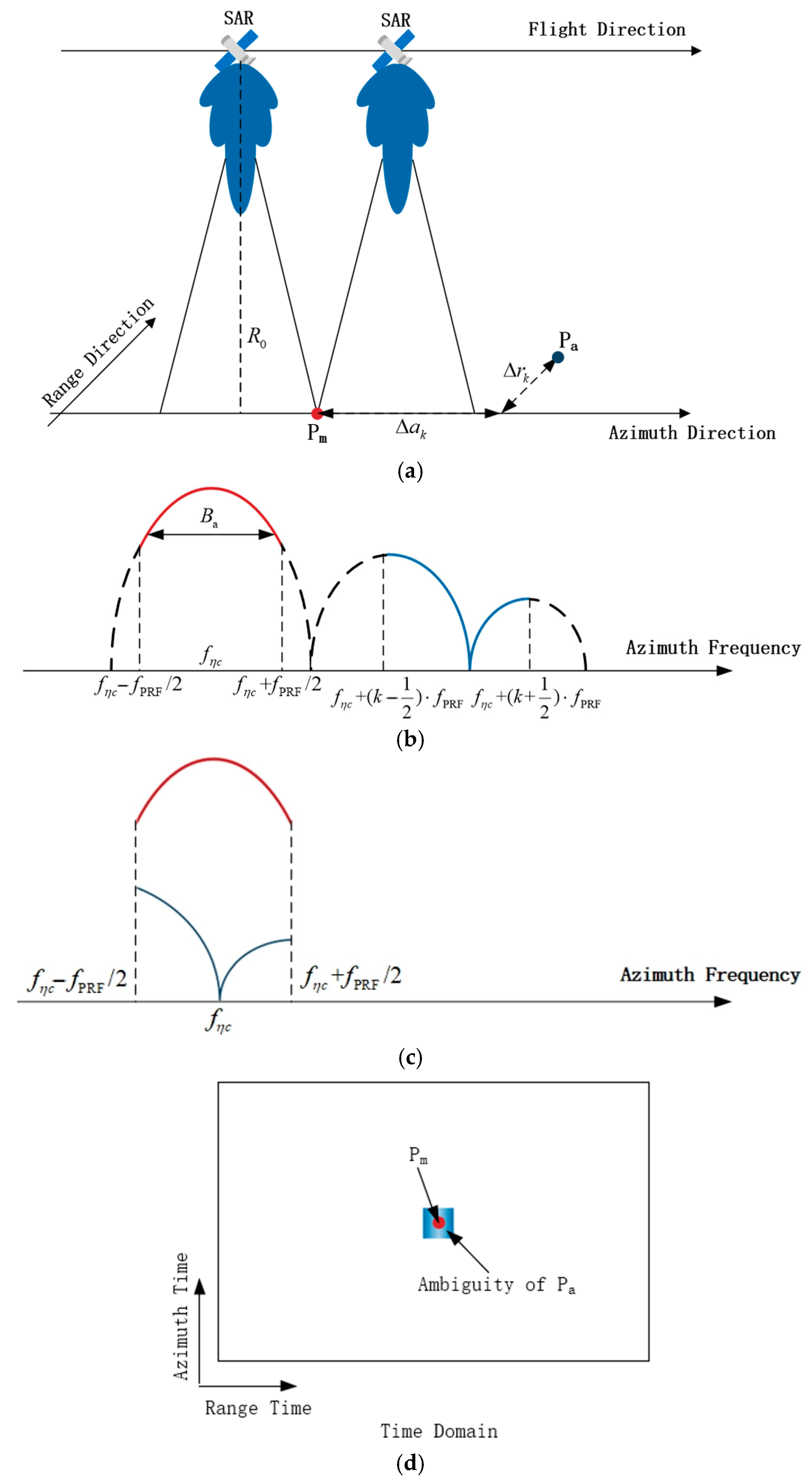
Figure 1a illustrates the schematic diagram of SAR observation during one synthetic aperture time $T_{\mathrm{a}}$. As the SAR platform moves from time $-T_{\mathrm{a}}/2$ to $T_{\mathrm{a}}/2$, point targets P_m and P_a remain within the antenna mainlobe and sidelobe, respectively. The relative position between P_m and P_a satisfies

$$\Delta a_k={\displaystyle \frac{k\lambda f_{\mathrm{PRF}}{R}_{\mathrm{N}}}{2v\cos \theta }},$$

(1)

and

$$\Delta r_k=R_0\sqrt{1-{\left(\sin \theta +{\displaystyle \frac{k\Delta a_k}{R_0}}\right)}^2}-R_{\mathrm{N}},$$

(2)

where $\Delta a_k$ is the relative distance between P_m and P_a in the azimuth direction, $\Delta r_k$ is the relative distance between P_m and P_a in the range direction, $R_{\mathrm{N}}$ is the closest range between SAR and P_m, $v$ is the relative velocity between SAR and the targets, $\theta$ is the squint angle forward from the orthonormal direction, $k$ represents the k-th ambiguous zone, and $R_0$ is the minimum of the range history of P_m.

The relative motion between SAR and the target generates the azimuth spectrum. The azimuth spectra of the point targets P_m and P_a are shown in Figure 1b, and their amplitudes are mainly determined by the azimuth pattern of the antenna, where $f_{\eta \mathrm{c}}$ represents the doppler center frequency, $B_{\mathrm{a}}$ is the spectral width corresponding to the 3 dB beam width of the antenna, and $f_{\mathrm{PRF}}$ is the pulse repetition frequency. The area containing echoes with azimuth frequencies in $\left[f_{\eta \mathrm{c}}-f_{\mathrm{PRF}}/2, f_{\eta \mathrm{c}}+f_{\mathrm{PRF}}/2\right]$ is called the main zone, while the area containing echoes with azimuth frequencies in $\left[f_{\eta \mathrm{c}}+\left(k-1/2\right)\cdot f_{\mathrm{PRF}}, f_{\eta \mathrm{c}}+\left(k+1/2\right)\cdot f_{\mathrm{PRF}}\right] \left(k\ne 0\right)$ is called the k-th ambiguous zone. Because SAR samples the echoes along the azimuth direction at the pulse repetition frequency and $f_{\mathrm{PRF}}$ is usually only 1.1 to 1.2 times $B_{\mathrm{a}}$ [10], the azimuth spectra of P_m and P_a inevitably undergo aliasing [11,12], as shown in Figure 1c. Correspondingly, azimuth ambiguity occurs in the time domain, as shown in Figure 1d.

Because the first ambiguous zone dominates 85% of the total ambiguous energy [13], this paper focuses exclusively on the case where $k=\pm 1$.

2.1. Azimuth Ambiguity in the Range-Time Azimuth-Frequency Domain

Suppose that in Figure 1a, P_m and P_a are respectively located in the main zone and the kth ambiguous zone. The range histories of P_m and P_a are $R_{\mathrm{rd}}\left(\eta \right)$ and $R_{\mathrm{ard}}\left(\eta \right)$, respectively. The minimum of $R_{\mathrm{rd}}\left(\eta \right)$ and $R_{\mathrm{ard}}\left(\eta \right)$ are $R_0$ and $R_{\mathrm{a}0}$, respectively.

The echo signal of P_m can be expressed as [1]

$$s\left(\tau ,\eta \right)={\sigma }_{\mathrm{M}}\cdot w_{\mathrm{r}}\left[\tau -{\displaystyle \frac{2R_{\mathrm{rd}}\left(\eta \right)}{c}}\right]\cdot w_{\mathrm{a}}\left(\eta -{\eta }_{\mathrm{c}}\right)\cdot \exp \left[-j{\displaystyle \frac{4\pi f_0{R}_{\mathrm{rd}}\left(\eta \right)}{\lambda }}\right]\cdot \exp \left\{j\pi K_{\mathrm{r}}{\left[\tau -{\displaystyle \frac{2R_{\mathrm{rd}}\left(\eta \right)}{c}}\right]}^2\right\},$$

(3)

where ${\sigma }_{\mathrm{m}}$ is the backscattering cross section of P_m, $w_{\mathrm{r}}$ is the range envelope, $w_{\mathrm{a}}$ is the azimuth envelope, $\tau$ is the range time, $\eta$ is the azimuth time, ${\eta }_c$ is the beam center crossing time, $f_0$ is the radar center frequency, $\lambda$ is the wavelength, and $K_{\mathrm{r}}$ is the range frequency modulation rate.

SAR imaging processors are typically designed for echoes from the main zone [7]. After imaging, the signal of P_m in the range-time azimuth-frequency domain takes the form [14]

$$S_0\left(\tau , f_{\eta }\right)={\sigma }_{\mathrm{M}}\cdot W_{\mathrm{a}}\left(f_{\eta }-f_{\eta \mathrm{c}}\right)\cdot \mathrm{Sin}\mathrm{c}\left(K_{\mathrm{r}}T\left(\tau -{\displaystyle \frac{2R_0}{c}}\right)\right),$$

(4)

where $f_{\eta }$ is the azimuth frequency, $W_{\mathrm{a}}$ is the azimuth antenna pattern, and $T$ is the transmitted pulse width.

In comparison, the signal of P_a in the range-time azimuth-frequency domain by applying the same image formation processing is

$$S_k\left(\tau , f_{\eta }\right)={\sigma }_{\mathrm{A}}\cdot W_{\mathrm{a}}\left(f_{\eta }+k\cdot f_{\mathrm{PRF}}-f_{\eta c}\right)\cdot \mathrm{Sin}\mathrm{c}\left[K_{r}T\left(\tau -{\tau }_k\right)\right],$$

(5)

where ${\sigma }_{\mathrm{A}}$ is the backscattering cross section of P_a, and ${\tau }_k$ can be denoted as

$${\tau }_k={\displaystyle \frac{2\left(R_0+S_{{\mathrm{ARCM}}_k}\right)}{c}}.$$

(6)

$S_{{\mathrm{ARCM}}_k}$ represents the residual range cell migration (RCM), which is defined as ambiguity range cell migration (ARCM) in [14,15], and can be approximately expressed as

$$S_{{\mathrm{ARCM}}_k}\left(R_0, f_{\eta }\right)=k\cdot R_0\left({\displaystyle \frac{c^2{f}_{\mathrm{PRF}}}{4v^2{f_0}^2}}{f}_{\eta }-{\displaystyle \frac{c^2{f_{\mathrm{PRF}}}^2}{8v^2{f}_0^2}}\right).$$

(7)

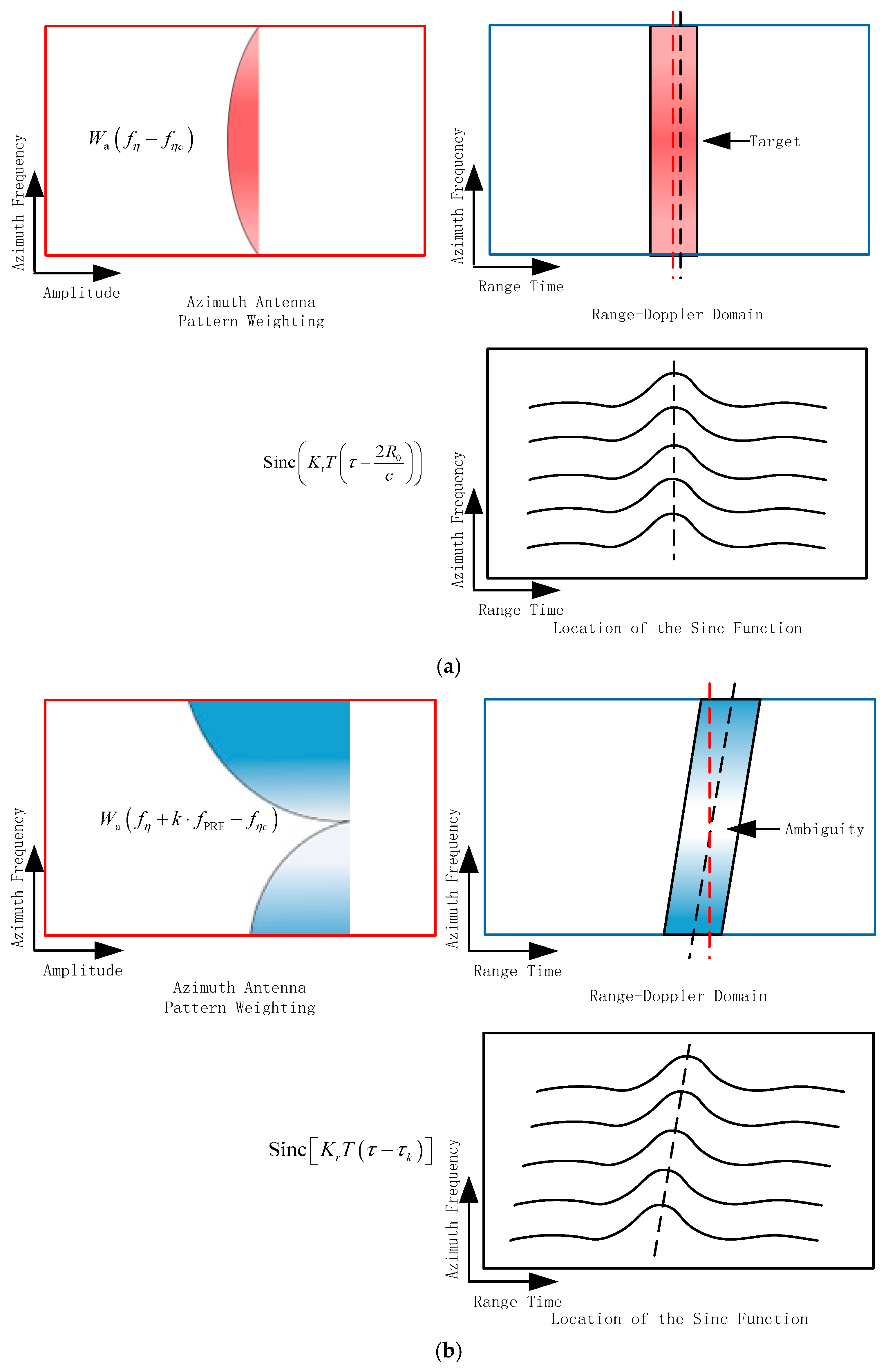
Figure 2 shows the range-time azimuth-frequency domain characteristics of P_m and P_a after imaging processing. The key distinctions are as follows:

(1)

Because the RCM correction and azimuth phase compensation in imaging are both designed for echoes from the main zone, the RCM of P_m is completely corrected, whereas residual linear terms related to azimuth frequency persist in the RCM of ambiguity signals. Consequently, in the range-time azimuth-frequency domain, signals corresponding to P_m exhibit distributions parallel to the azimuth direction, while ambiguity signals are distributed at an incline.

(2)

The signals from the main zone are primarily weighted by the 3 dB azimuth mainlobe of the antenna pattern, whereas the ambiguity signals are weighted by antenna sidelobes. Due to the small fluctuation in the 3 dB mainlobe and significant fluctuations in the sidelobes, the intensity variation of the main zone signal is small, while that of the azimuth ambiguity signal is obvious.

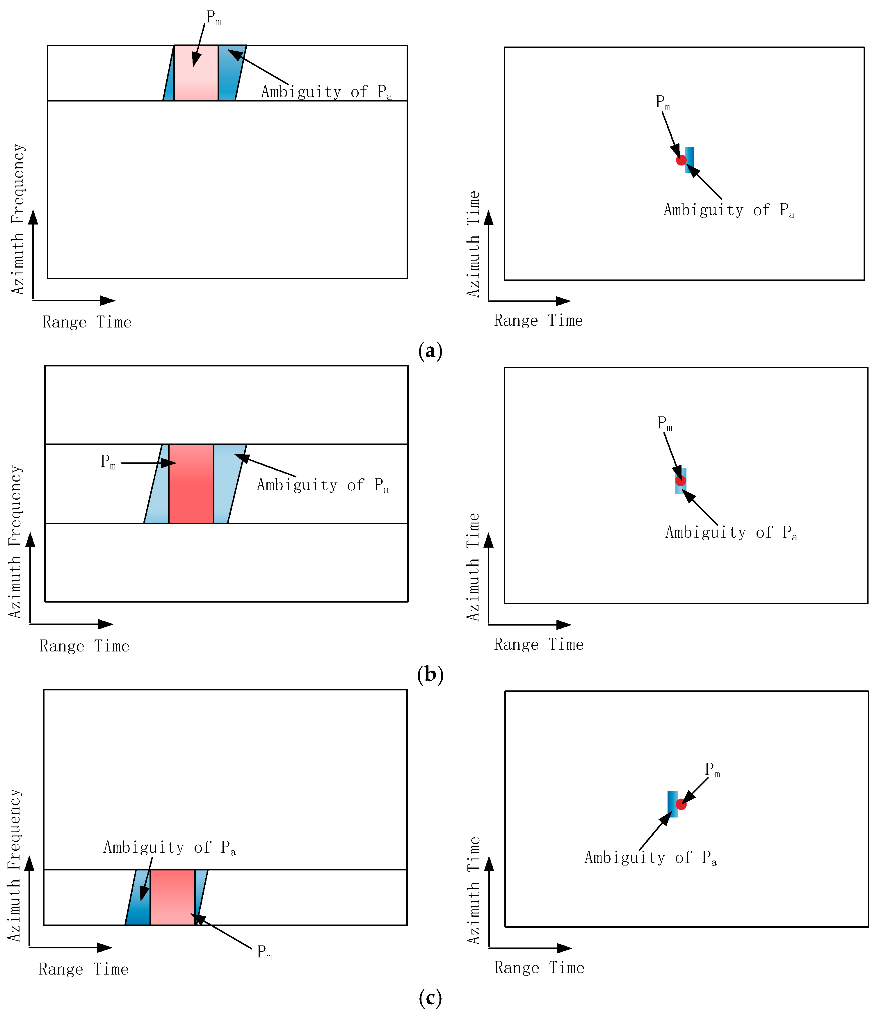
Based on the above two characteristics, if the main zone signals in Equation (4) and the ambiguity signals in Equation (5) are segmented into multiple sub-spectra along the azimuth direction and transformed to the azimuth time domain, they exhibit the following properties:

(1)

The time-domain images of main zone signals remain nearly identical across different azimuth sub-spectra.

(2)

The time-domain images of ambiguity signals show positional shifts and significant intensity variations between different azimuth sub-spectra, as illustrated in Figure 3. Consequently, by selecting the time-domain image of a sub-spectrum with minimal ambiguity energy and performing change detection against time-domain images of other sub-spectra, the spatial positions of azimuth ambiguities in each azimuth sub-spectrum’s time domain can be determined.

The above properties are shown in Figure 3.

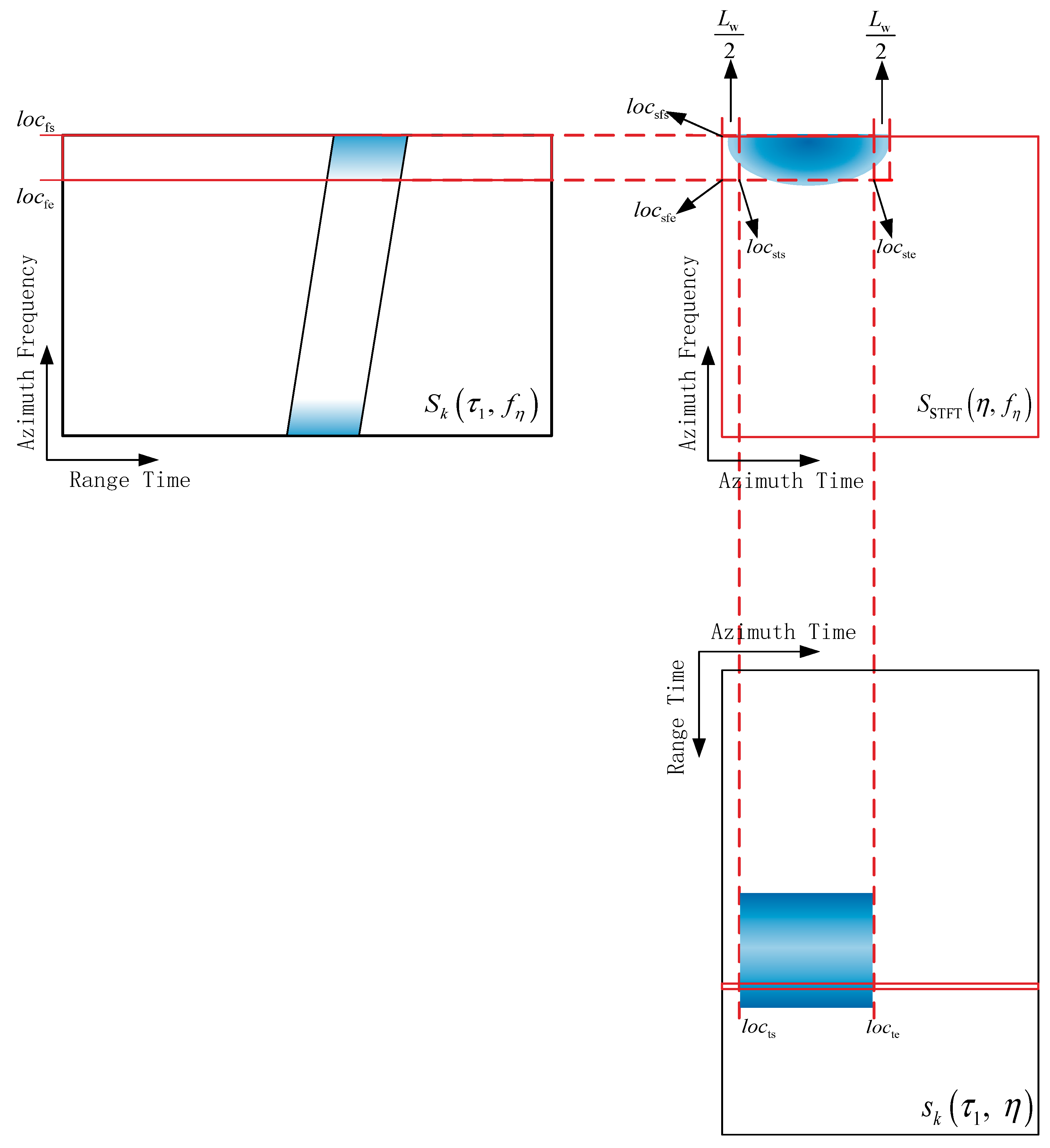
2.2. Azimuth Ambiguity in Azimuth Time-Frequency Domain

In the range-time azimuth-time domain, time-frequency transformation is performed on the azimuth ambiguity signal within the range bin ${\tau }_1$ to obtain its representation in the azimuth time-frequency domain. The input of the time-frequency transformation is a range bin from the SAR image data containing ambiguity after imaging processing. The output of time-frequency transformation is a two-dimensional plane containing the information of the range bin in the image. One dimension represents azimuth time, and the other dimension represents azimuth frequency. The time-frequency transformation adopted in the paper is short-time Fourier transform [16,17]:

$$S_{\mathrm{STFT}}\left(\eta , f_{\eta }\right)={\displaystyle \underset{-\infty }{\overset{+\infty }{\int }}{s}_k\left({\tau }_1, t\right)w\left(t-\eta \right)e^{-j2\pi f_{\eta }t}dt},$$

(8)

where $s_k\left({\tau }_1, \eta \right)$ is the inverse Fourier transform of $S_k\left({\tau }_1, f_{\eta }\right)$, $w\left(t-\eta \right)$ is the Hamming window centered on the azimuth time $\eta$.

From Equation (8), the signal characteristics in the azimuth time-frequency domain are mainly determined by $s_k\left({\tau }_1, t\right)w\left(t-\eta \right)$. If the length of the Hamming window $w\left(t-\eta \right)$ is $L_{\mathrm{w}}$, the ambiguous energy over the region

$$R_{\mathrm{STFT}}=\left\{\left(\eta , f_{\eta }\right)|lo{c}_{\mathrm{sts}}\le \eta \le lo{c}_{\mathrm{ste}}, lo{c}_{\mathrm{sfs}}\le f_{\eta }\le lo{c}_{\mathrm{sfe}}\right\}$$

(9)

in $S_{\mathrm{STFT}}\left(\eta , f_{\eta }\right)$ is mapped to the region

$$R_T=\left\{\eta |lo{c}_{\mathrm{ts}}\le \eta \le lo{c}_{\mathrm{te}}\right\}$$

(10)

in $s_k\left({\tau }_1, t\right)$.

Combining Equation (5) and the distribution area described by Equation (10), the corresponding region in $S_k\left({\tau }_1, f_{\eta }\right)$ is

$$R_F=\left\{f_{\eta }|lo{c}_{\mathrm{fs}}\le f_{\eta }\le lo{c}_{\mathrm{fe}}\right\},$$

(11)

where

$$lo{c}_{\mathrm{sts}}=lo{c}_{\mathrm{ts}}-L_{\mathrm{w}}/2,$$

(12)

$$lo{c}_{\mathrm{ste}}=lo{c}_{\mathrm{te}}+L_{\mathrm{w}}/2,$$

(13)

$$lo{c}_{\mathrm{sfs}}=lo{c}_{\mathrm{fs}},$$

(14)

and

$$lo{c}_{\mathrm{sfe}}=lo{c}_{\mathrm{fe}}.$$

(15)

The relationship between Equations (9)–(15) is shown in Figure 4.

Based on Equations (12)–(15), the positions of azimuth ambiguities can be detected in the range-time azimuth-time domain and then precisely suppressed in the azimuth time-frequency domain.

3. Time-Frequency Joint Detection and Suppression Method

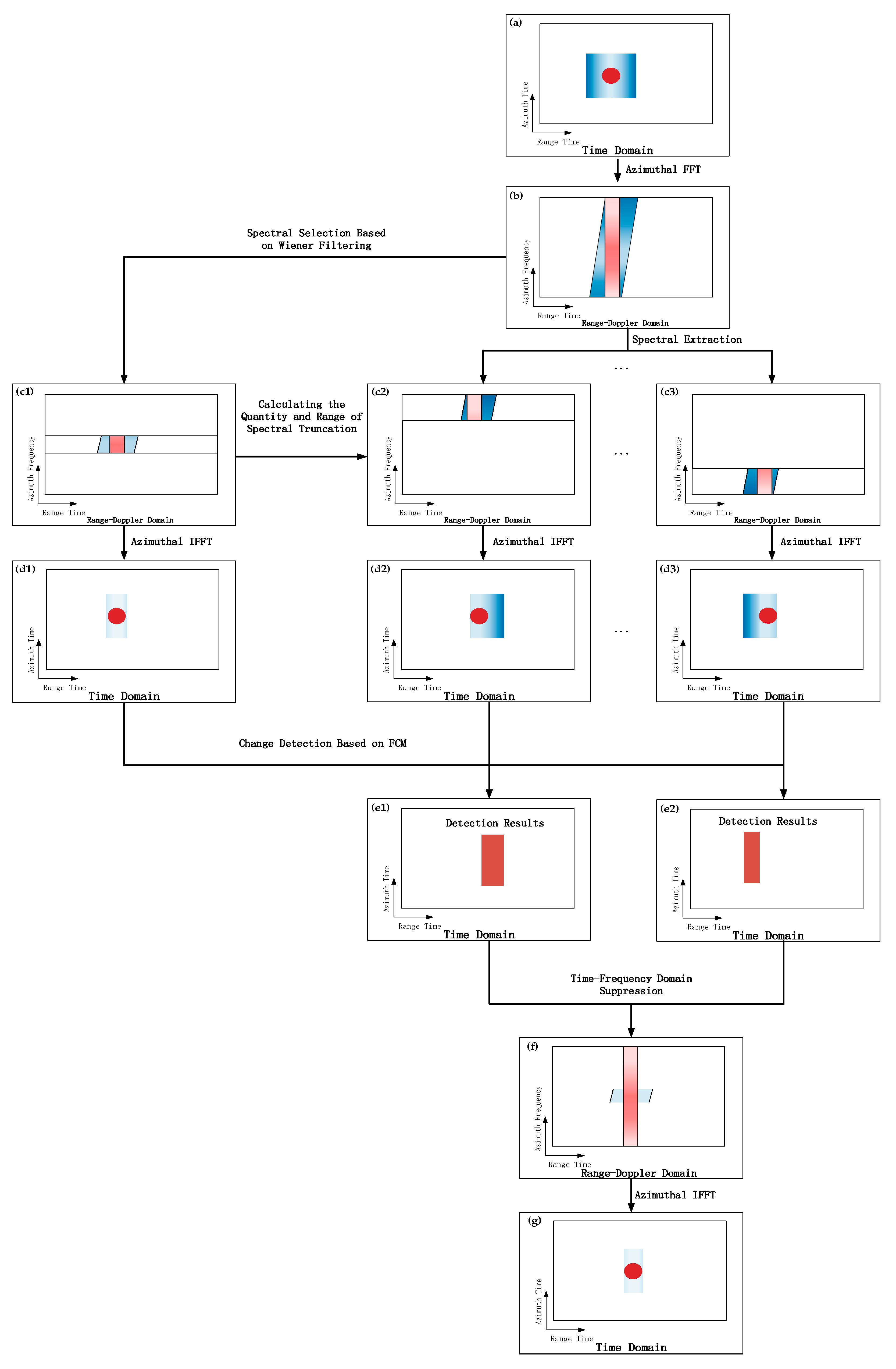
Based on the characteristics of the azimuth ambiguity signals in Section 2, this section proposes a joint time-frequency method for detecting and suppressing azimuth ambiguities. In Figure 5, the process of joint time-frequency detection and suppression of azimuth ambiguity is expounded in the form of a diagram. Firstly, spectral selection is carried out using the Wiener filter, which is obtained by estimating the local azimuth ambiguity to signal ratios and the azimuth antenna pattern to obtain a sub-spectrum with less ambiguity. Then, this sub-spectrum is taken as the reference spectrum and truncation is performed on the original spectrum through the width of the reference spectrum. The images corresponding to the obtained different sub-spectra and that correspond to the reference spectrum are subjected to change detection based on the fuzzy C-means clustering method. The fuzzy C-means algorithm determines the change category by inputting the logarithmic ratio difference image of two images and continuously clustering and iterating. Finally, the detection results of different sub-spectra are fused to obtain the azimuth ambiguity detection results.

3.1. Azimuth Ambiguity Signal Detection

The analysis in Section 2.1 demonstrates that azimuth ambiguities can be localized by comparing images from different azimuth sub-spectra. To ensure detection performance, it is necessary to select a sub-spectrum with lower ambiguity energy to construct a reference image.

The Wiener filter $H^{\mathrm{wiener}}$ is constructed as follows:

$$\begin{array}{cc}{H}^{\mathrm{wiener}}& ={\displaystyle \frac{{\sigma }_{\mathrm{ma}}^2|W_{\mathrm{a}}(f_{\eta }){|}^2}{{\sigma }_{\mathrm{ma}}^2|W_{\mathrm{a}}(f_{\eta }){|}^2+{\displaystyle {\sum }_{k=\pm 1}{\sigma }_{ak}^2|W_{\mathrm{a}}(f_{\eta }+k{f}_{\mathrm{PRF}}){|}^2}}}\hfill \\ & \approx {\left[\begin{array}{l}1+LAAS{R}_{+1}{\displaystyle \frac{{\displaystyle {\int }_{-B_{\mathrm{a}}/2}^{B_{\mathrm{a}}/2}|W_{\mathrm{a}}(f_{\eta }){|}^{2}d{f}_{\eta }}}{{\displaystyle {\int }_{-B_{\mathrm{a}}/2}^{B_{\mathrm{a}}/2}|W_{\mathrm{a}}(f_{\eta }+f_{\mathrm{PRF}}){|}^{2}d{f}_{\eta }}}}{\displaystyle \frac{|W_{\mathrm{a}}(f_{\eta }+f_{\mathrm{PRF}}){|}^2}{|W_{\mathrm{a}}(f_{\eta }){|}^2}}\\ +LAAS{R}_{-1}{\displaystyle \frac{{\displaystyle {\int }_{-B_{\mathrm{a}}/2}^{B_{\mathrm{a}}/2}|W_{\mathrm{a}}(f_{\eta }){|}^{2}d{f}_{\eta }}}{{\displaystyle {\int }_{-B_{\mathrm{a}}/2}^{B_{\mathrm{a}}/2}|W_{\mathrm{a}}(f_{\eta }-f_{\mathrm{PRF}}){|}^{2}d{f}_{\eta }}}}{\displaystyle \frac{|W_{\mathrm{a}}(f_{\eta }-f_{\mathrm{PRF}}){|}^2}{|W_{\mathrm{a}}(f_{\eta }){|}^2}}\end{array}\right]}^{-1}\hfill \end{array},$$

(16)

where ${\sigma }_{\mathrm{ma}}$ is the backscattering cross-section of the main zone, ${\sigma }_{ak}$ is the backscattering cross-section of the ambiguity zone, and $LAAS{R}_{+1}$ and $LAAS{R}_{-1}$ are the local azimuth ambiguity-to-signal ratios (local AASR) corresponding to the +1st and −1st ambiguous zones, respectively [18,19,20]. Local AASR is defined as the ratio of ambiguous energy to ambiguity-free energy in specific regions such as the +1st or −1st ambiguous zones. For detailed calculation, refer to [8,18].

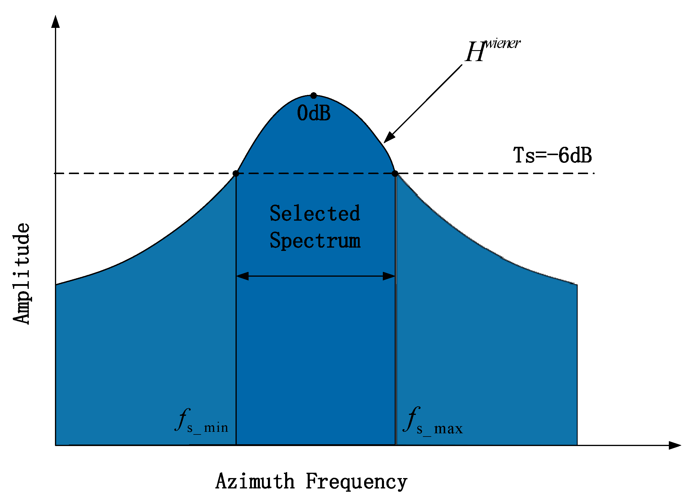
The Wiener filter undergoes normalization, as illustrated in Figure 6. A threshold, typically set at −6 dB, is applied to identify the azimuth frequency band exceeding this threshold, which is denoted as $\left[f_{\mathrm{s}\_\min }, f_{\mathrm{s}\_\max }\right]$. The value −6 dB was obtained through experimental experience. In fact, within the range of −7 dB to −5 dB, it can be ensured that the truncated spectrum has the characteristics of little ambiguity and appropriate spectral width and can be used as reference spectra. This sub-spectrum is then designated as the reference spectrum, and its bandwidth is recorded as

$$f_{\mathrm{width}}=f_{\mathrm{s}\_\max }-f_{\mathrm{s}\_\min }.$$

(17)

After transforming the imaging domain into the range-time azimuth-frequency domain, the number of sub-spectra obtained after azimuth spectrum partitioning is

$$N_{\mathrm{fre}}=⌈{\displaystyle \frac{f_{\mathrm{PRF}}}{f_{\mathrm{width}}}}⌉,$$

(18)

where $⌈\cdot ⌉$ is ceiling. The frequencies of the m-th sub-spectrum are

$$\left[f_{\eta \mathrm{c}}-f_{\mathrm{PRF}}/2+\left(m-1\right)\cdot f_{\mathrm{width}}, f_{\eta \mathrm{c}}-f_{\mathrm{PRF}}/2+m\cdot f_{\mathrm{width}}\right] 1\le m\le N_{\mathrm{fre}}.$$

(19)

Each sub-spectrum is transformed back to the azimuth time domain via inverse Fourier transform and normalized to obtain the corresponding image $s_{\mathrm{f}, m}\left(1\le m\le N_{\mathrm{fre}}\right)$. The sub-image corresponding to the reference spectrum is denoted as $s_{\mathrm{ba}}$. The difference image is calculated using the logarithmic ratio between $s_{\mathrm{f}, m}$ and $s_{\mathrm{ba}}$. Then, the fuzzy C-means clustering method is adopted for the different images to obtain the differences between $s_{\mathrm{f}, m}$ and $s_{\mathrm{ba}}$. By fusing the detection results, the positions of all azimuth ambiguities in the range-time azimuth-time domain are determined.

3.2. Azimuth Ambiguity Signal Suppression

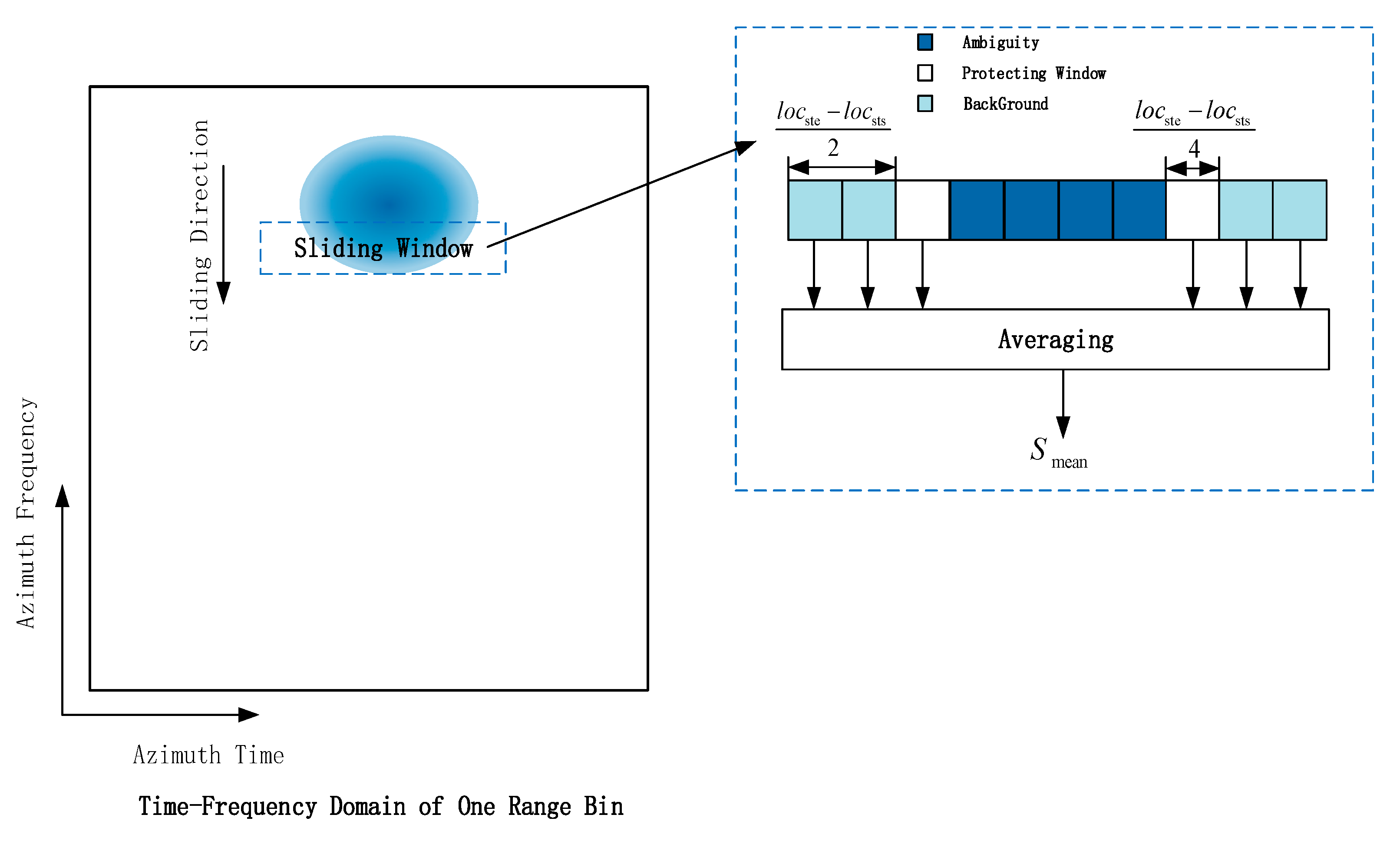
Based on the positions of azimuth ambiguity signals in the range-time azimuth-time domain and Equations (12)–(15), the approximate distribution of azimuth ambiguity signals in the azimuth time-frequency domain of each range bin can be determined. Subsequently, sliding-window filtering is applied to achieve azimuth ambiguity suppression.

The sliding window is illustrated in Figure 7. The sliding window size is set to $\left(lo{c}_{\mathrm{ste}}-lo{c}_{\mathrm{sts}}\right)\cdot ⌈f_{\mathrm{width}}/Z_{\mathrm{s}}⌉$. The length of this sliding window in the azimuth time dimension is determined by the azimuth ambiguity detection results. The sliding window performs ambiguity suppression along the azimuth frequency dimension. $Z_{\mathrm{s}}$ serves as the windowing coefficient, where a larger $Z_{\mathrm{s}}$ results in a smaller window. Typically, the detected time-frequency energy width $\left(lo{c}_{\mathrm{ste}}-lo{c}_{\mathrm{sts}}\right)$ is used as a reference. A guard band of size $\left(lo{c}_{\mathrm{ste}}-lo{c}_{\mathrm{sts}}\right)/4$ and a background band of size $\left(lo{c}_{\mathrm{ste}}-lo{c}_{\mathrm{sts}}\right)/2$ are set on both sides of the window. The sliding window starts moving from the minimum frequency with a step size of $⌈f_{\mathrm{width}}/Z_{\mathrm{s}}⌉$. During each movement, the average energy in the background band is calculated and denoted as $S_{\mathrm{mean}}$. The energy suppression threshold is set as follows:

$$T_{\mathrm{su}}=Z_{\mathrm{e}}\cdot S_{\mathrm{mean}},$$

(20)

where $Z_{\mathrm{e}}$ is the threshold suppression coefficient. The smaller $Z_{\mathrm{e}}$ is, the stronger the suppression effect becomes. The signals within the sliding window are processed according to the following equation:

$$H_{\mathrm{su}}\left(i,j\right)=\left\{\begin{array}{l}S\left(i,j\right){\left|S\left(i,j\right)\right|}^2<T_{\mathrm{su}}\\ S\left(i,j\right)\cdot N_{\mathrm{su}}{\left|S\left(i,j\right)\right|}^2\ge T_{\mathrm{su}}\end{array}\right.,$$

(21)

where $S\left(i,j\right)$ is the azimuth time-frequency signal at $\left(i,j\right)$ and $N_{\mathrm{su}}$ is the suppression factor computed by

$$N_{\mathrm{su}}={\displaystyle \frac{\sqrt{T_{\mathrm{su}}}}{\left|S\left(i,j\right)\right|}}$$

(22)

The suppressed result is obtained by transforming the azimuth time-frequency data after sliding window processing to the range-time azimuth-time domain.

4. Experimental Results

This section evaluates the proposed algorithm by using two airborne SAR datasets and compares them with the classical asymmetric mapping and selective filtering method (AM&SF) [1] and the spectral selection and extrapolation method (SS&E) [8].

In the AM&SF method, selective filtering is obtained by using Wiener filters to identify the areas polluted by azimuth ambiguities. After the generation of ambiguity maps, asymmetric selective filters are used to suppress the ambiguity based on the evaluation of local signal-to-ambiguity ratios. Compared with the AM&SF method, the ambiguity suppression effect of the proposed method is better than that of AM&SF method, especially when the generation of ambiguity does not come from one ambiguous zone.

The SS&E method creates a model to describe the azimuth antenna pattern weighting on azimuth ambiguity. Based on this model, the algorithm can better estimate the ratio of ambiguous to ambiguity-free energy to obtain a better spectral selection effect. Then, extrapolation is performed on the selected spectra to obtain the image after ambiguity suppression. Although both the SS&E method and the proposed method involve spectrum selection, the spectrum selection requirements of the proposed method are less restrictive compared to those of SS&E and can retain more valid information and target details in the spectra discarded by SS&E.

4.1. Data and Parameters

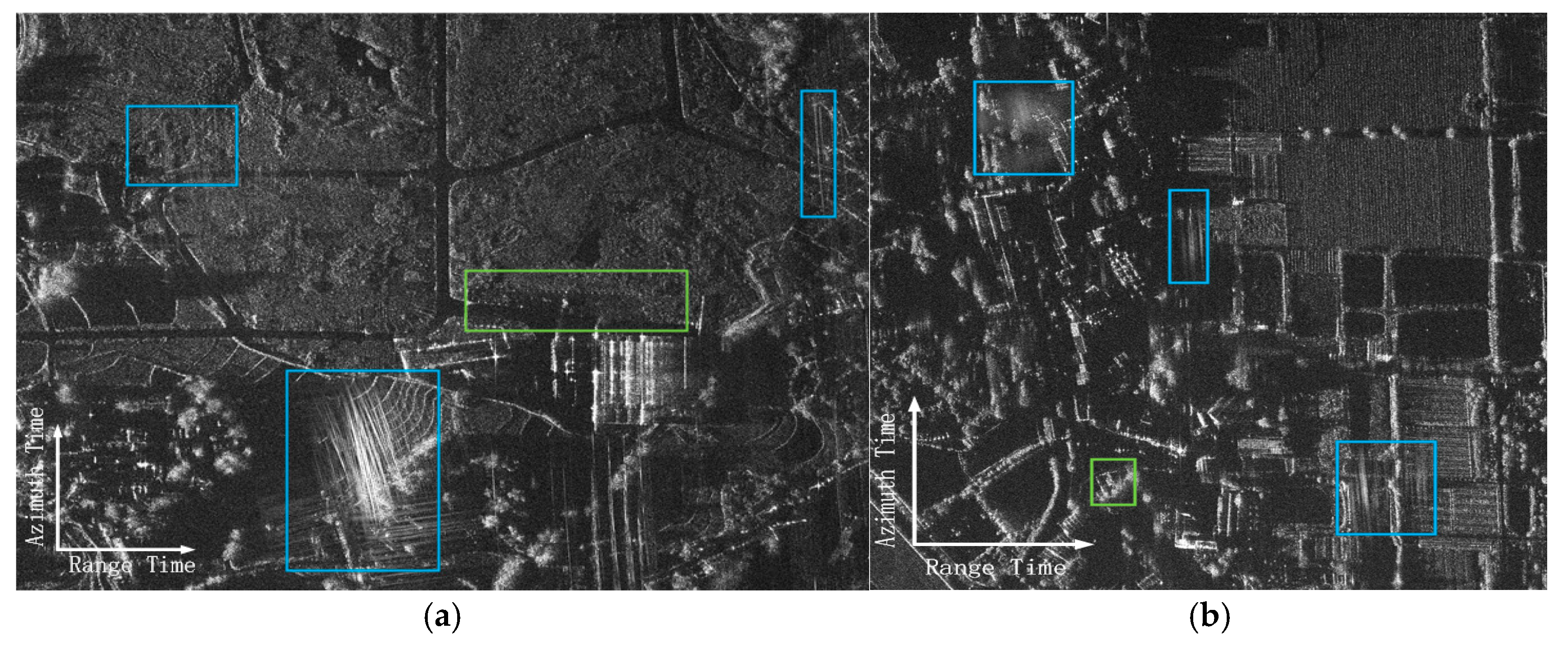
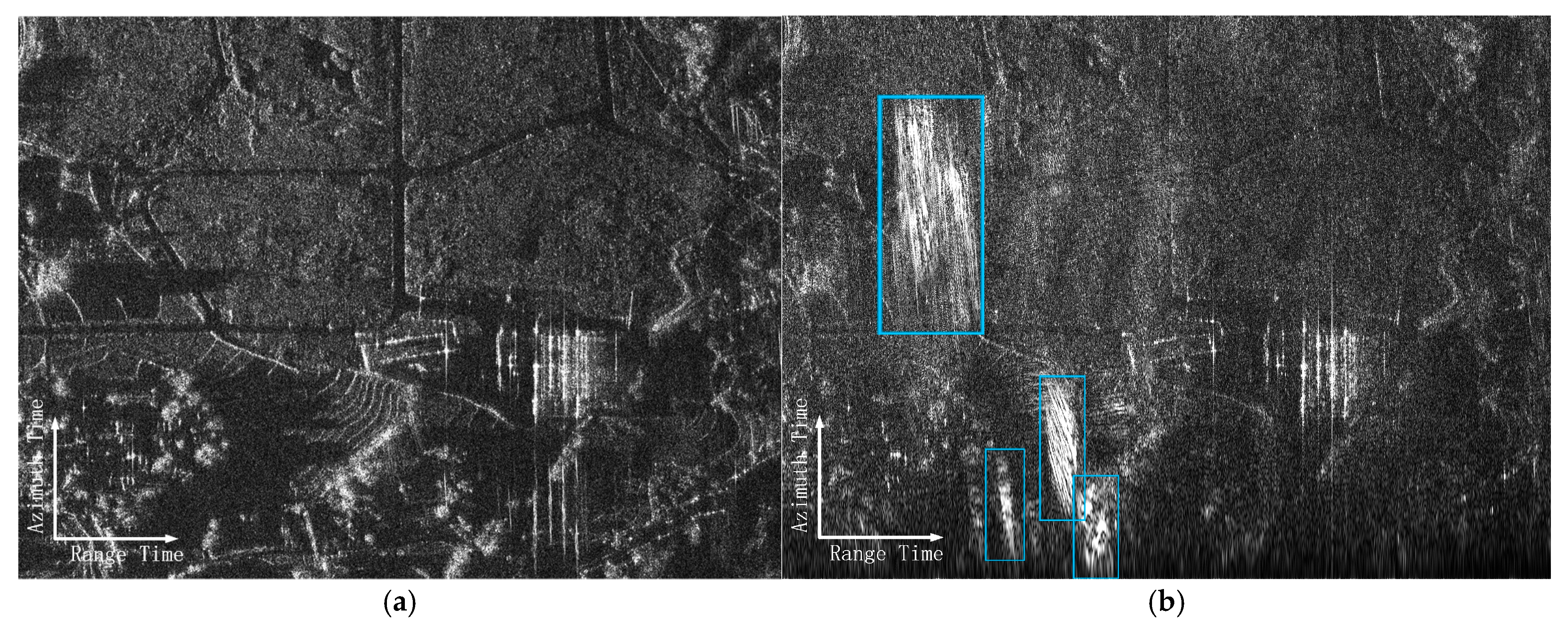
The SAR data used in the experiment are shown in Figure 8. These data were obtained using airborne SAR in Chongqing, China in March 2024. The parameters of these data are shown in

Table 1. Experimental data parameters.

Parameter Name	Value
Signal bandwidth	600 MHz
Pulse repetition frequency (PRF)	600 Hz
Radar azimuth 3 dB bandwidth	459.6 Hz
Carrier velocity	68.85 m/s
Radar frequency	9.6 GHz
Nearest slant range	19701 m

.

In Figure 8, the regions marked by blue boxes exhibit significant azimuth ambiguity. Furthermore, the azimuth ambiguity is superimposed over true targets, severely degrading the imaging quality of real features such as farmland and mountainous areas. The regions marked by green boxes contain multiple point targets and small structures, which were used to evaluate the preservation capability of the proposed method for true targets.

4.2. Results of Azimuth Ambiguity Suppression

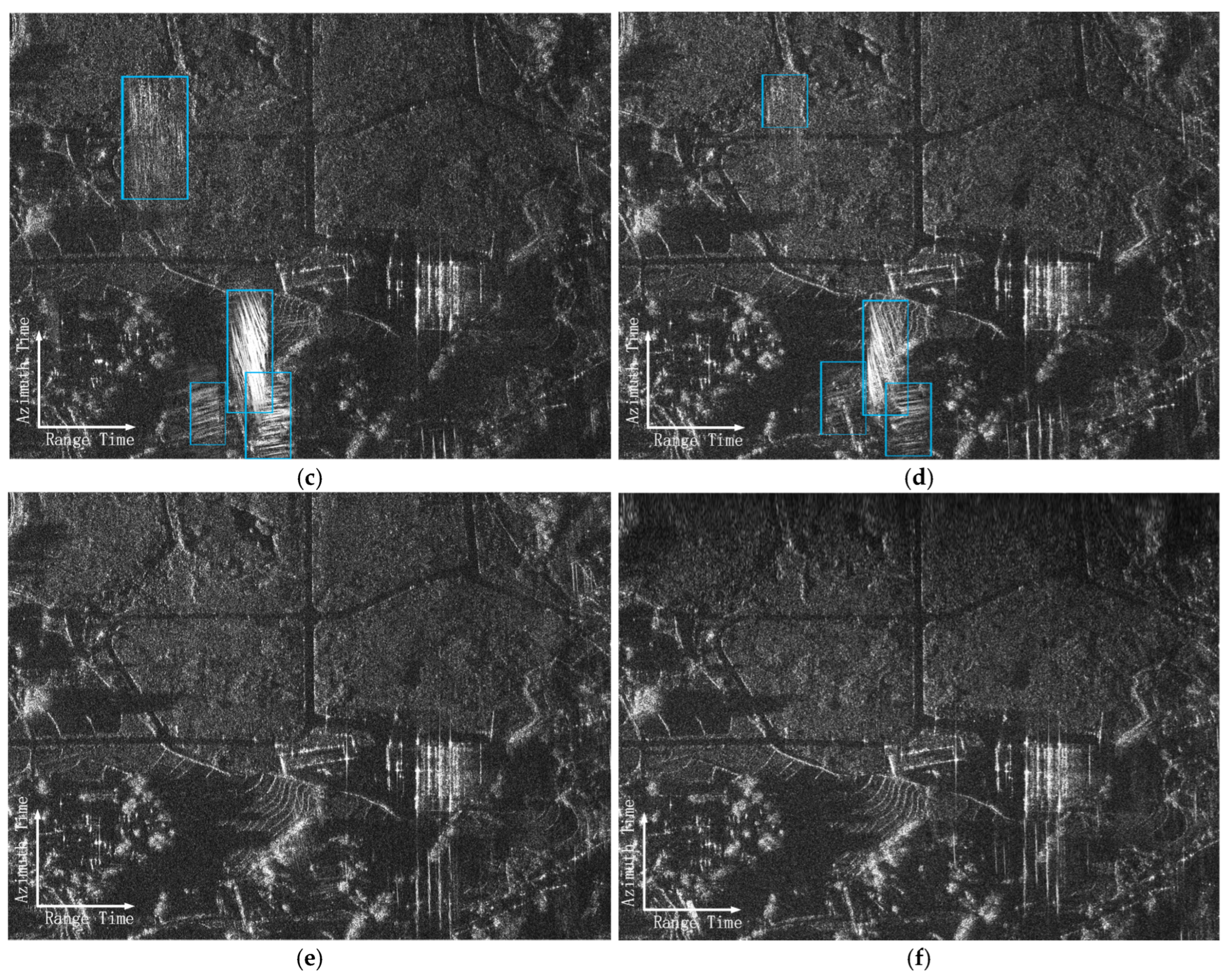
The Wiener filter shown in Equation (15) was employed to estimate the azimuth ambiguity distribution for Figure 8a. According to the estimation of the Wiener filter, the image corresponding to the frequency band [−32 Hz, 48 Hz] was selected as the reference image, as shown in Figure 9a. This image contains low azimuth ambiguity energy. By calculating the spectral width of the selected spectrum, the truncation range of each sub-spectrum of the original spectrum was determined. Figure 9b–f display the images corresponding to the frequency bands [−280 Hz, −200 Hz], [−200 Hz, −120 Hz], [−120 Hz, −40 Hz], [−40 Hz, 40 Hz], and [40 Hz, 120 Hz], respectively. These images represent the real targets and ambiguity energy contained in the different sub-spectra. Significant azimuth ambiguities can be observed in Figure 9b–d, as highlighted by the blue boxes.

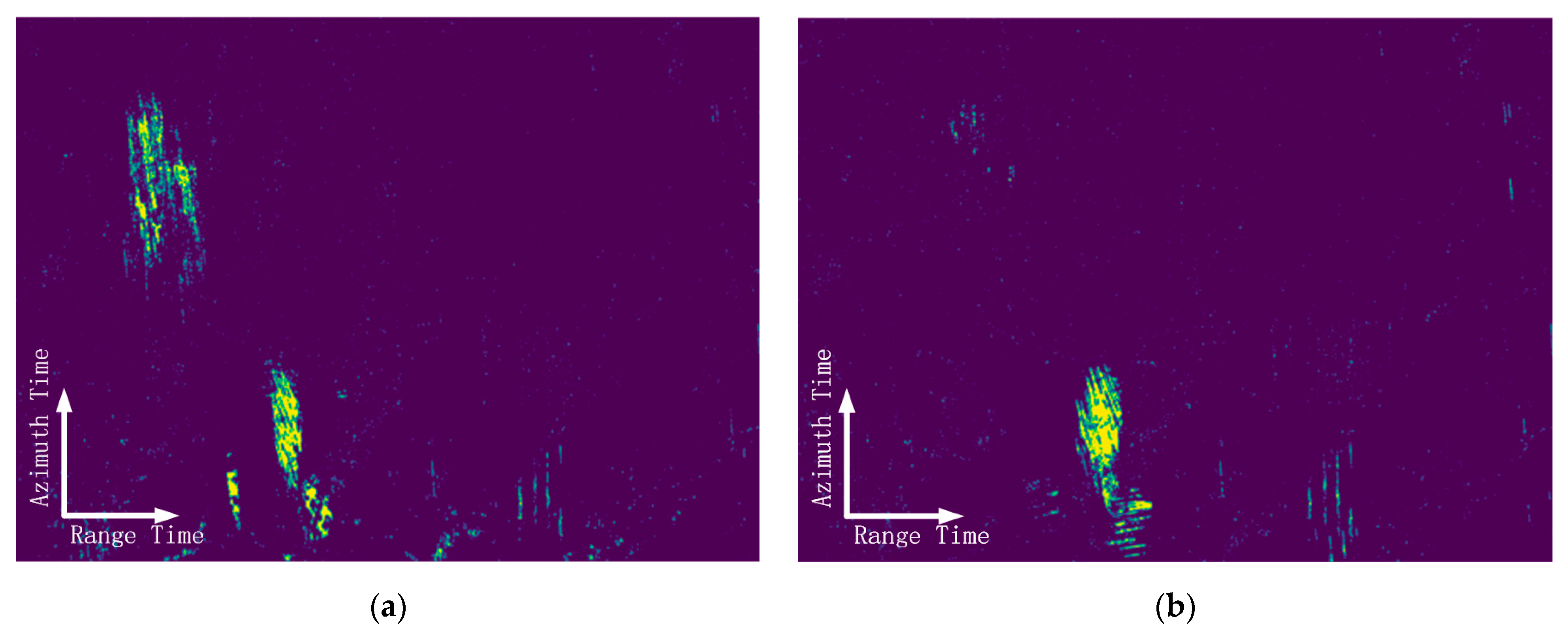
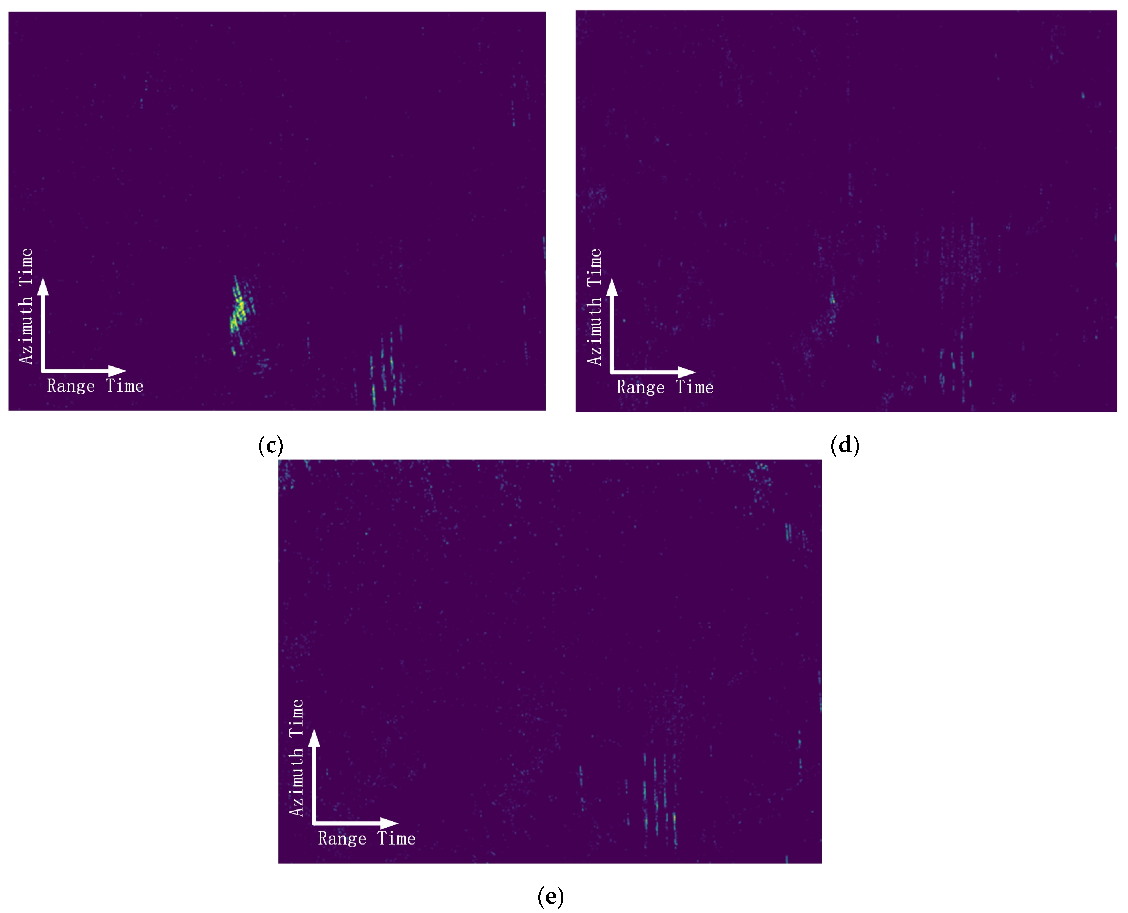
Figure 10a–e demonstrates the change detection results between the reference image in Figure 9a and the images of different sub-spectra which are shown in Figure 9b–f. The change detection results are also the detection results of azimuth ambiguity in each sub-spectrum.

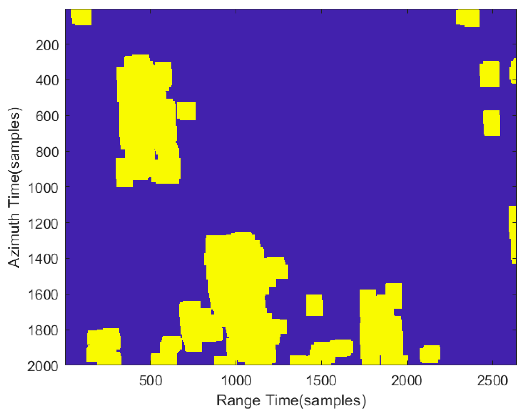
The detection results of each sub-spectrum were fused to obtain a complete azimuth ambiguity detection result in yellow blocks, as shown in Figure 11.

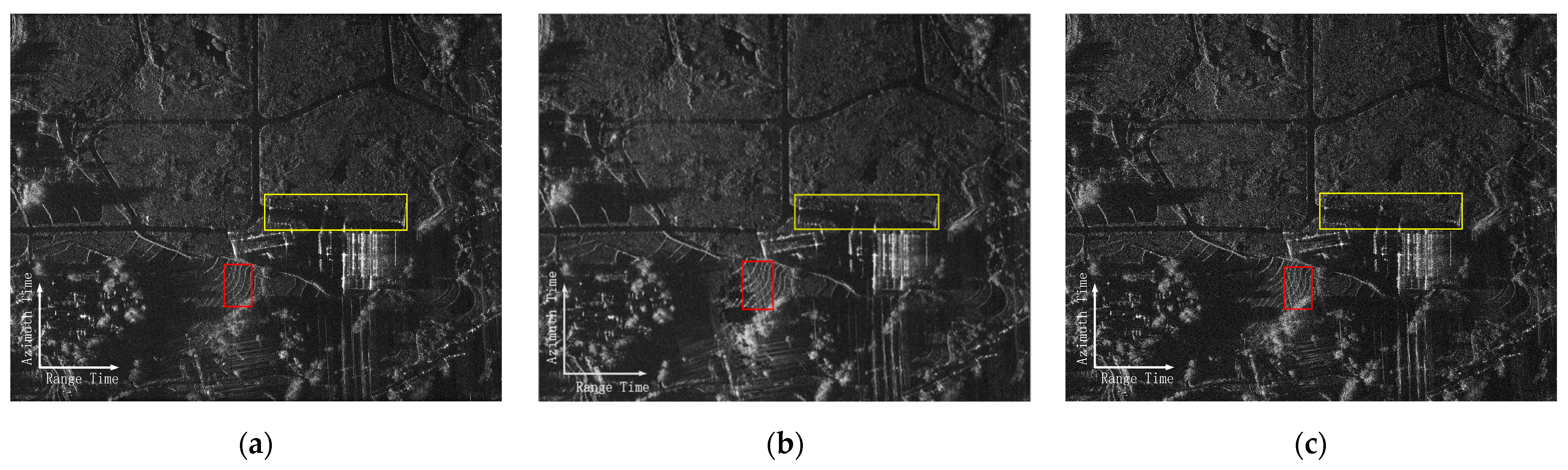
Each range bin in the data shown in Figure 8a was transformed into the azimuth time-frequency domain, and the method described in Section 3.2 was applied to suppress azimuth ambiguity signals. The AM&SF method and SS&E method were also implemented for comparison. The corresponding results are presented in Figure 12. By evaluating the ambiguity-to-signal ratio within the red-boxed region of Figure 12 (as summarized in

Table 2. Comparison results of azimuth ambiguity-to-signal ratio.

Method	Azimuth Ambiguity-to-Signal Ratio of the Data in Figure 8a	Azimuth Ambiguity-to-Signal Ratio of the Data in Figure 8b
Original Data	−7.9519 dB	−19.7098 dB
Proposed Method	−10.8028 dB	−24.9625 dB
AM&SF	−8.9377 dB	−21.5091 dB
SS&E	−10.1716 dB	−22.0092 dB

), it is demonstrated that the proposed method outperforms the AM&SF method in azimuth ambiguity suppression by 1.8651 dB and outperforms the SS&E method in azimuth ambiguity suppression by 0.6312 dB.

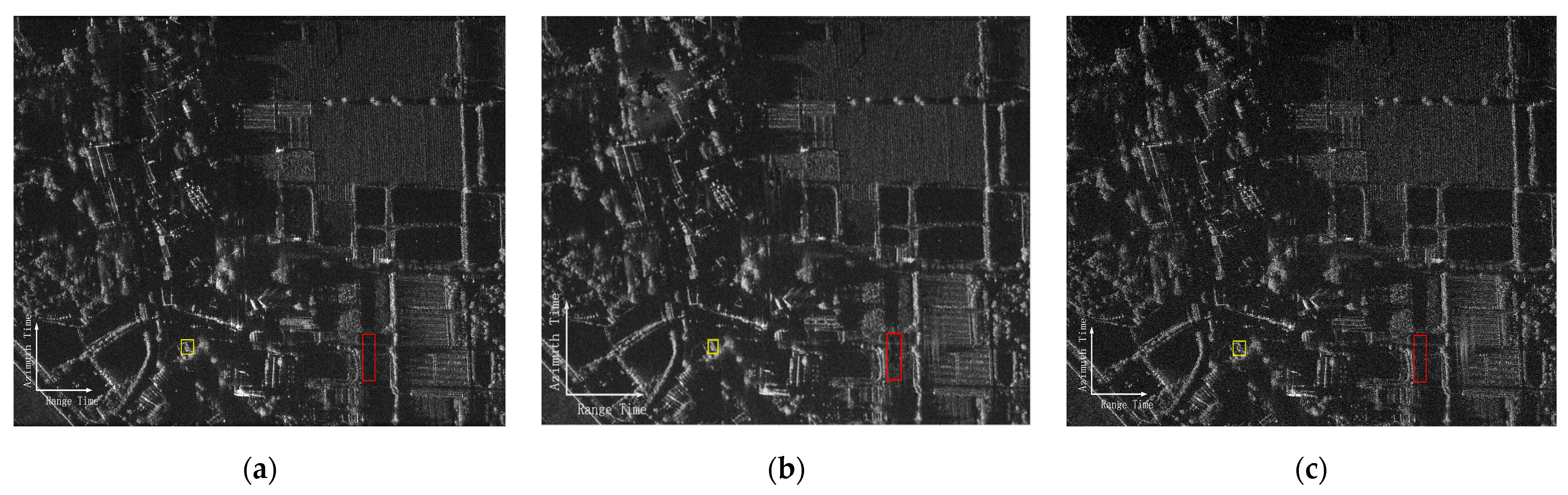
The proposed method, the AM&SF method and the SS&E method were also applied to suppress the azimuth ambiguity in Figure 8b, and the results are shown in Figure 13. By evaluating the ambiguity-to-signal ratio within the red-boxed region of Figure 13 (as summarized in Table 2), it is demonstrated that the proposed method outperforms the AM&SF method in azimuth ambiguity suppression by 3.4534 dB and the proposed method outperforms the SS&E method in azimuth ambiguity suppression by 2.9533 dB.

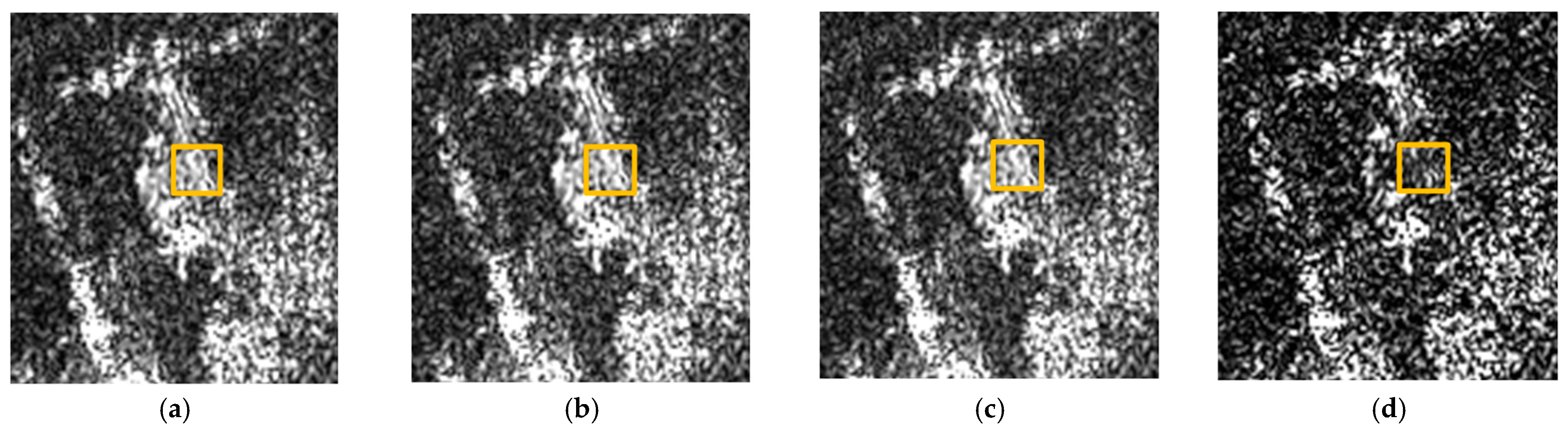
4.3. Results of Real Target Preservation

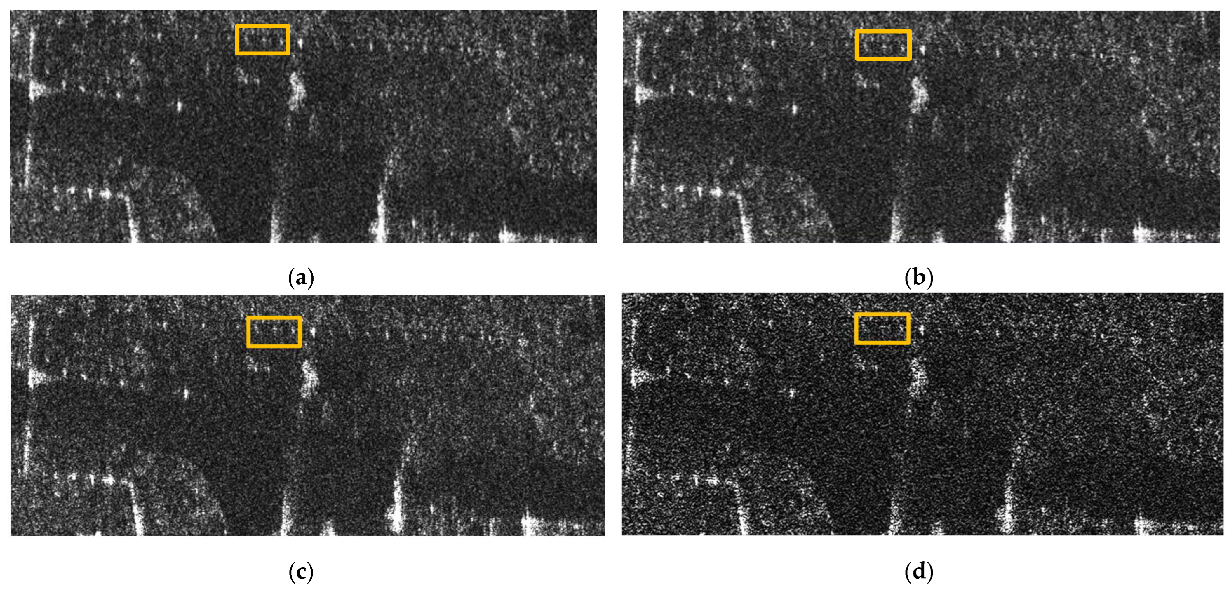
Figure 14a displays an enlarged view of the green-boxed region in Figure 8a, illustrating the original state of targets prior to ambiguity suppression. Figure 14b displays an enlarged view of the yellow-boxed region in Figure 12a. Figure 14c displays an enlarged view of the yellow-boxed region in Figure 12b. Figure 14d displays an enlarged view of the yellow-boxed region in Figure 12c.

The result processed by the proposed method demonstrates complete retention of point-like targets within the orange box, as shown in Figure 14b. The result processed by the AM&SF method is also similar to the original image in terms of target retention within the orange box, as shown in Figure 14c. In contrast, the result processed by the SS&E method exhibits noticeable target loss in the corresponding areas, as shown in Figure 14d.

Figure 15a displays an enlarged view of the green-boxed region in Figure 8b, where the orange frame highlights a part of a building. Figure 15b displays an enlarged view of the yellow-boxed region in Figure 13a. Figure 15c displays an enlarged view of the yellow-boxed region in Figure 13b. Figure 15d displays an enlarged view of the yellow-boxed region in Figure 13c. The result processed by the proposed method demonstrates complete retention of architectural details within the orange boxes, as shown in Figure 15b. The result processed by the AM&SF method is also similar to the original image in terms of target retention within the orange box, as shown in Figure 15c. In contrast, the result processed by the SS&E method exhibits significant degradation of structural features in the building in Figure 15d.

5. Discussion

Although the proposed method has a similar target retention effect to the AM&SF method, the proposed method demonstrates superior performance over the AM&SF in ambiguity suppression. The suppression effect of the AM&SF method significantly declines when suppressing ambiguity from different ambiguous zones. The proposed method demonstrates superior performance over the SS&E method in both ambiguity suppression and target preservation. Furthermore, after calculation, there is not much difference between SS&E and the proposed method in terms of resolution maintenance. The azimuth resolution of the proposed method is basically consistent with that of the original image. The primary limitation of the SS&E method lies in its spectral truncation and extrapolation operations, which inadvertently attenuate the energy intensity of the true targets. In contrast, the time-frequency joint method proposed in this paper is designed to preserve true targets while suppressing ambiguities through the time-frequency domain. Compared to conventional time-domain or frequency-domain processing, time-frequency joint suppression is more refined and is able to achieve a better balance between ambiguity suppression and target preservation.

6. Conclusions

Because the PRF of SAR echo signals is smaller than the bandwidth of the azimuth spectrum, spectral aliasing occurs in the azimuth spectrum inevitably, resulting in azimuth ambiguity which can severely degrade SAR image quality. This paper has proposed a method based on joint time-frequency analysis for azimuth ambiguity suppression. This method performs change detection on images of different sub-spectra to obtain the distribution of azimuth ambiguity in the image and then completes ambiguity suppression in the time-frequency domain. Because the time-frequency domain contains more detailed information compared to the image domain and the frequency domain, the proposed method provides more precise suppression on the spectrum based on joint time-frequency analysis compared to classic ambiguity suppression algorithms such as the AM&SF method and the SS&E method. Experiments on airborne SAR data proved that the proposed method is superior to the AM&SF method and the SS&E method in terms of azimuth ambiguity suppression. Furthermore, the proposed method outperforms the SS&E method in terms of the retention effect of real target details.

References

- Di Martino, G.; Iodice, A.; Riccio, D.; Ruello, G. Filtering of azimuth ambiguity in stripmap synthetic aperture radar images. IEEE J. Sel. Top. Appl. Earth Obs. Remote Sens. 2014, 7, 3967–3978. [Google Scholar] [CrossRef]
- Raney, R.K.; Princz, G.J. Reconsideration of azimuth ambiguities in SAR. IEEE Trans. Geosci. Remote Sens. 1987, 6, 783–787. [Google Scholar] [CrossRef]
- Horiuchi, R.; Hoshino, T.; Oishi, N.; Suwa, K. Azimuth ambiguity discrimination using Doppler spectrum of the compressive sensing-based SAR image with downsampled PRF. In Proceedings of the 2020 17th European Radar Conference (EuRAD), Utrecht, The Netherlands, 13–15 January 2021; pp. 318–321. [Google Scholar]
- Santamaria, C.; Greidanus, H. Ambiguity discrimination for ship detection using Sentinel-1 repeat acquisition operations. In Proceedings of the 2015 IEEE International Geoscience and Remote Sensing Symposium (IGARSS), Milan, Italy, 26–31 July 2015; pp. 2477–2480. [Google Scholar]
- Bordoni, F.; Younis, M.; Krieger, G. Ambiguity suppression by azimuth phase coding in multichannel SAR systems. IEEE Trans. Geosci. Remote Sens. 2011, 50, 617–629. [Google Scholar] [CrossRef]
- Moreira, A. Suppressing the azimuth ambiguities in synthetic aperture radar images. IEEE Trans. Geosci. Remote Sens. 1993, 31, 885–895. [Google Scholar] [CrossRef]
- Guarnieri, A.M. Adaptive removal of azimuth ambiguities in SAR images. IEEE Trans. Geosci. Remote Sens. 2005, 43, 625–633. [Google Scholar] [CrossRef]
- Wu, Y.; Yu, Z.; Xiao, P.; Li, C. Suppression of azimuth ambiguities in spaceborne SAR images using spectral selection and extrapolation. IEEE Trans. Geosci. Remote Sens. 2018, 56, 6134–6147. [Google Scholar] [CrossRef]
- Xuejiao, W.; Xiaolan, Q.; Lei, C.; Jiyun, W.; Qi, C. An improved azimuth ambiguity suppression method for SAR based on ambiguity area imaging and detection. IEEE J. Sel. Top. Appl. Earth Obs. Remote Sens. 2022, 15, 8155–8169. [Google Scholar] [CrossRef]
- Cumming, I.G.; Wong, F.H. Digital processing of synthetic aperture radar data. Artech house 2005, 1, 108–110. [Google Scholar]
- Li, F.; Johnson, W. Ambiguities in spacebornene synthetic aperture radar systems. IEEE Trans. Aerosp. Electron. Syst. 1983, 3, 389–397. [Google Scholar] [CrossRef]
- Velotto, D.; Soccorsi, M.; Lehner, S. Azimuth ambiguities removal for ship detection using full polarimetric X-band SAR data. IEEE Trans. Geosci. Remote Sens. 2013, 52, 76–88. [Google Scholar] [CrossRef]
- Zhang, Z.; Wang, Z.-s. On suppressing azimuth ambiguities of synthetic aperture radar by three filters. In Proceedings of the 2001 CIE International Conference on Radar Proceedings (Cat No. 01TH8559), Beijing, China, 15–18 October 2001; pp. 624–626. [Google Scholar]
- Suo, Y.; Fu, K.; Wu, Y.; Diao, W.; Dai, W.; Sun, X. A parameter-free enhanced SS&E algorithm based on deep learning for suppressing azimuth ambiguities. IEEE Trans. Geosci. Remote Sens. 2022, 61, 5200316. [Google Scholar]
- Chen, J.; Wang, K.; Yang, W.; Liu, W. Accurate reconstruction and suppression for azimuth ambiguities in spaceborne stripmap SAR images. IEEE Geosci. Remote Sens. Lett. 2016, 14, 102–106. [Google Scholar] [CrossRef]
- Zhang, R.; Li, G.; Zhang, Y.D. Micro-Doppler interference removal via histogram analysis in time-frequency domain. IEEE Trans. Aerosp. Electron. Syst. 2016, 52, 755–768. [Google Scholar] [CrossRef]
- Stankovic, L.; Thayaparan, T.; Dakovic, M.; Popovic-Bugarin, V. Micro-Doppler removal in the radar imaging analysis. IEEE Trans. Aerosp. Electron. Syst. 2013, 49, 1234–1250. [Google Scholar] [CrossRef]
- Villano, M.; Krieger, G. Spectral-based estimation of the local azimuth ambiguity-to-signal ratio in SAR images. IEEE Trans. Geosci. Remote Sens. 2013, 52, 2304–2313. [Google Scholar] [CrossRef]
- Ren, Y.; Zheng, M.; Yin, Z. An azimuth ambiguity suppression method based on ambiguity focusing for SAR-GMTI. IEEE Geosci. Remote Sens. Lett. 2023, 20, 4014305. [Google Scholar] [CrossRef]
- Long, Y.; Zhao, F.; Zheng, M.; Jin, G.; Zhang, H. An azimuth ambiguity suppression method based on local azimuth ambiguity-to-signal ratio estimation. IEEE Geosci. Remote Sens. Lett. 2020, 17, 2075–2079. [Google Scholar] [CrossRef]
Figure 1.
Schematic diagram of SAR azimuth ambiguity generation. (a) Shows SAR observation within the synthetic aperture time ; (b) is the azimuth spectra of the unaliased point targets Pm and Pa, where the blue line represents the spectrum corresponding to Pa and the red line represents the spectrum corresponding to Pm. The colors in (c) have the same meaning; (c) demonstrates that the azimuth spectra of Pm and Pa are aliased, resulting in azimuth ambiguity; (d) illustrates the imaging domain of Pm and Pa. Pm is focused while Pa is defocused.
Figure 2.
The range-time azimuth-frequency domain characteristics of points Pm and Pa. (a) The blue box represents characteristic of Pm in the range-time azimuth-frequency domain, the red box shows the weighting of the antenna pattern, and the black box describes the Sinc function in Equation (4). (b) The blue box represents the characteristic of Pa in the range-time azimuth-frequency domain. The red box shows the weighting of the antenna pattern, and the black box describes the Sinc function in Equation (5). The depth of color represents the strength of the energy. In contrast, the distribution of the ambiguity signal in the range-time azimuth-frequency domain is inclined, and the energy in different azimuth sub-spectra shows obvious differences.
Figure 3.
Schematic diagram of image domains corresponding to different azimuth sub-spectra. The left column shows the distribution of points Pm and Pa in different azimuth sub-spectra, while the right column displays the corresponding image domain. Red represents the main zone signal, blue represents azimuth ambiguity signals, with color depth representing energy intensity. By comparing (a–c), it can be observed that the imaging of main zone signals remains essentially consistent across different sub-spectra, while azimuth ambiguity signals exhibit positional shifts and intensity variations in different azimuth sub-spectra.
Figure 4.
Diagram showing relationships among the range-time azimuth-time domain, range-time azimuth-frequency domain and azimuth time-frequency domain. The depth of color represents the strength of energy.
Figure 5.
Schematic diagram of the joint time-frequency algorithm for detecting and suppressing azimuth ambiguities. (a) represents that the image domain contains an ambiguity which is shown in blue and a real target which is shown in red; (b) is the azimuth Fourier transform result of (a); (c1) represents the result of spectrum selection, while (c2) and (c3) are the spectra truncated based on the spectral width of (c1); (d1–d3) are the inverse azimuth Fourier transform results of (c1–c3) respectively; (e1) is the change detection result between (d1) and (d2); (e2) is the change detection result between (d1) and (d3); (f) is the ambiguity suppression result in range-time azimuth-frequency domain; (g) is the ambiguity suppression result in image domain.
Figure 6.
Spectral selection using a Wiener filter.
Figure 7.
Ambiguity suppression using sliding window in azimuth time-frequency domain.
Figure 8.
The experimental SAR data which were used for validation. (a) Ambiguity data 1 with ambiguity covering farmlands; (b) ambiguity data 2 with ambiguity covering buildings.
Figure 9.
Images corresponding to the extracted sub-spectra from experimental data. (a) Image corresponding to the sub-spectrum selected via the Wiener filter; (b–f) images corresponding to the frequency bands: [−280 Hz, −200 Hz], [−200 Hz, −120 Hz], [−120 Hz, −40 Hz], [−40 Hz, 40 Hz], and [40 Hz, 120 Hz], respectively.
Figure 10.
Time-frequency joint detection results. (a–e) Correspond to the change detection results of the images of different sub-spectra, respectively.
Figure 11.
The fusion map of detection results of different sub-spectra, where the yellow regions represent the area where azimuth ambiguity signals exist.
Figure 12.
Comparison of the results of different azimuth ambiguity suppression methods for the data shown in
Figure 8a. (
a) Suppression results of the proposed method; (
b) suppression results of the AM&SF method; (
c) suppression results of the SS&E method.
Figure 13.
Figure 8b. (
Figure 14.
The retention situation of the targets in
a) Original data; (
b) suppression results of the proposed method; (
c) suppression results of the AM&SF method; (
d) suppression results of the SS&E method.
Figure 15.