
Spatiotemporal Dynamic Changes in Cropland and Multi-Scenario Simulation in the Yarlung Zangbo River Basin

 ,
,  , , ,
, , ,
Abstract
1. Introduction
2. Materials and Methods
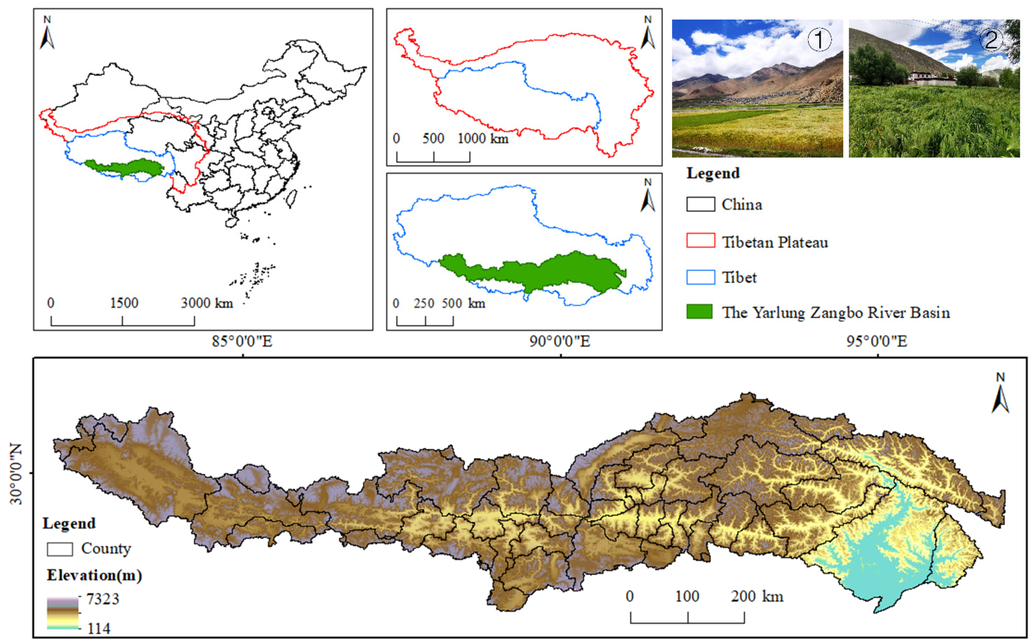
2.1. Study Area
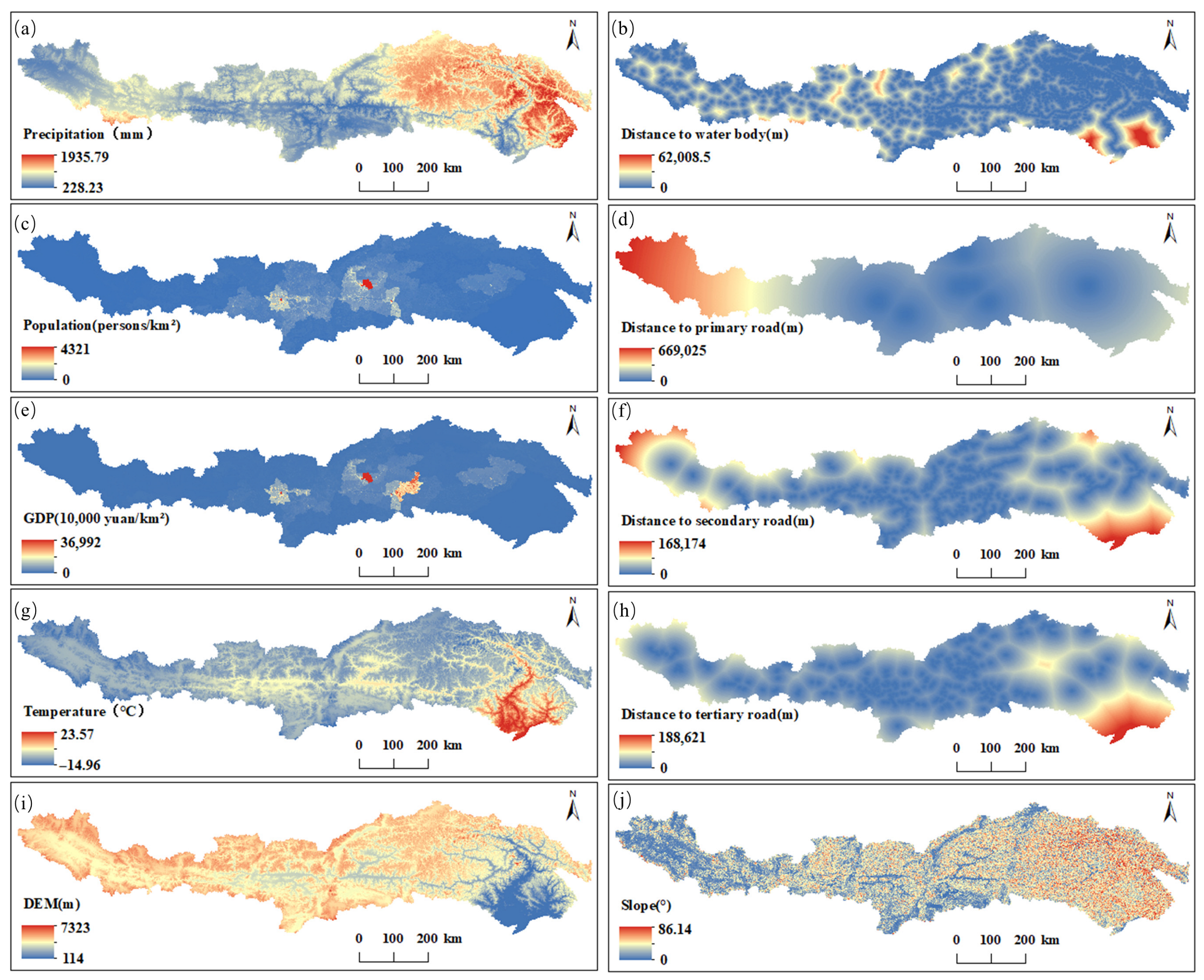
2.2. Data Sources
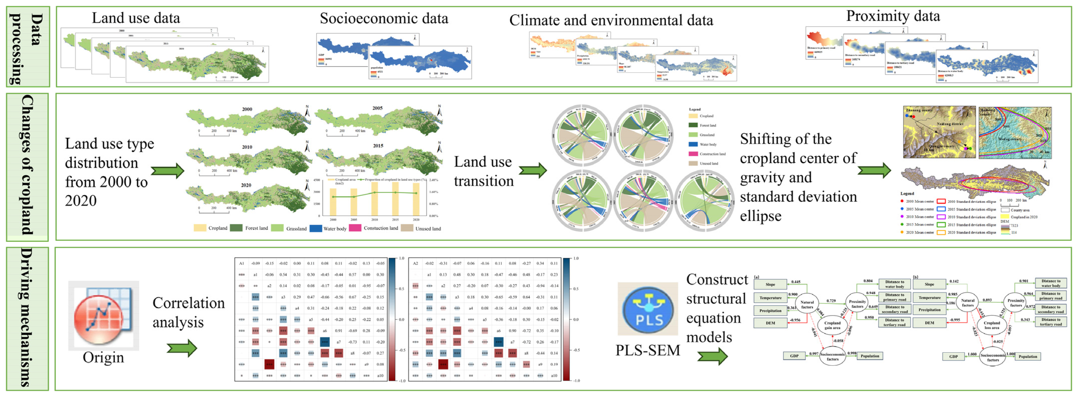
2.3. Methods
2.3.1. Land Use Transition Matrix
2.3.2. Land Use Dynamic Degree
2.3.3. Center of Gravity Model
2.3.4. Standard Deviation Ellipse
2.3.5. PLS-SEM
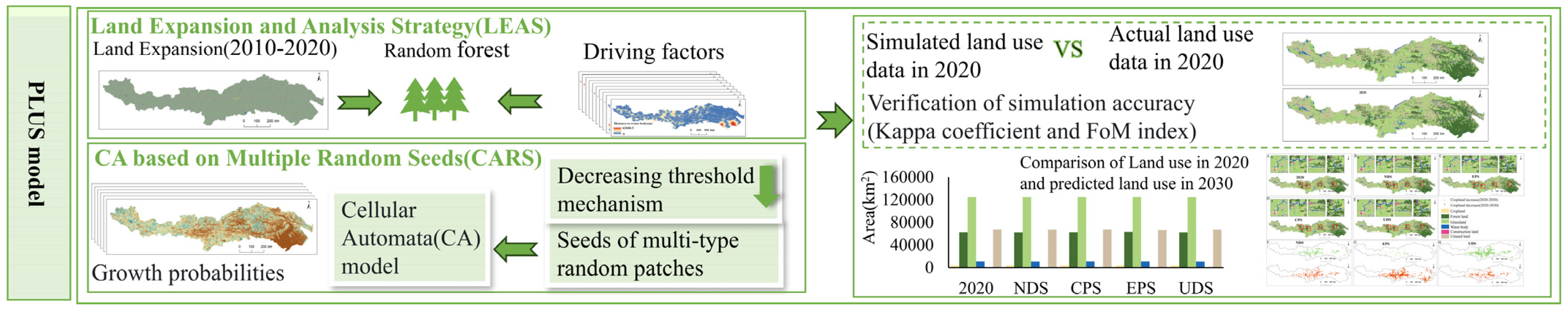
2.3.6. PLUS Model
- (1)
- Natural development scenario (NDS): Based on the evolution of land types in the YZRB from 2000 to 2020, the Markov chain in the PLUS model is used to predict land use demand in the YZRB for 2030, without setting the probabilities of mutual conversion between land categories [51].
- (2)
- Urban development scenario (UDS): The probability of conversion from cropland, forestland, grassland, and unused land to construction land is increased by 20%, while the probability of conversion from construction land to other land types, excluding cropland, is decreased by 30% [52].
- (3)
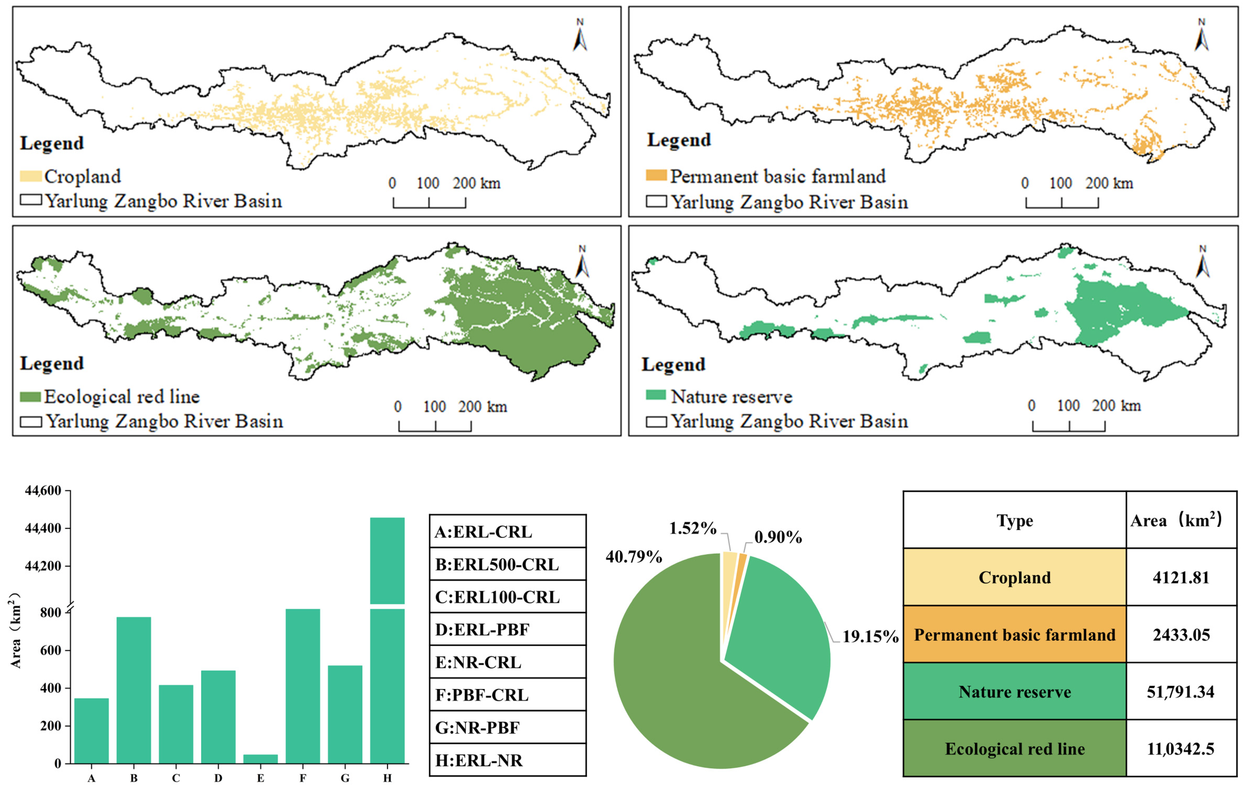
- Ecological protection scenario (EPS): Except for construction land, all other land use categories are allowed to convert to forestland and grassland. To enhance ecological conservation, the probability of conversion from forestland and grassland to construction land was reduced by 50%, and that from cropland to construction land was reduced by 30%. Meanwhile, the probability of conversion from cropland and grassland to forestland increased by 30% [53]. Additionally, natural reserves and areas within ecological red lines were defined as restricted zones where land use transitions are not permitted.
- (4)
- Cropland protection scenario (CPS): Cropland is the foundation for ensuring food supply and food security. The probability of conversion from forestland and grassland to construction land is reduced by 20%, and the probability of conversion from cropland to construction land is reduced by 60% [54,55]. Permanent basic cropland is set as a conversion–restricted zone.
3. Results
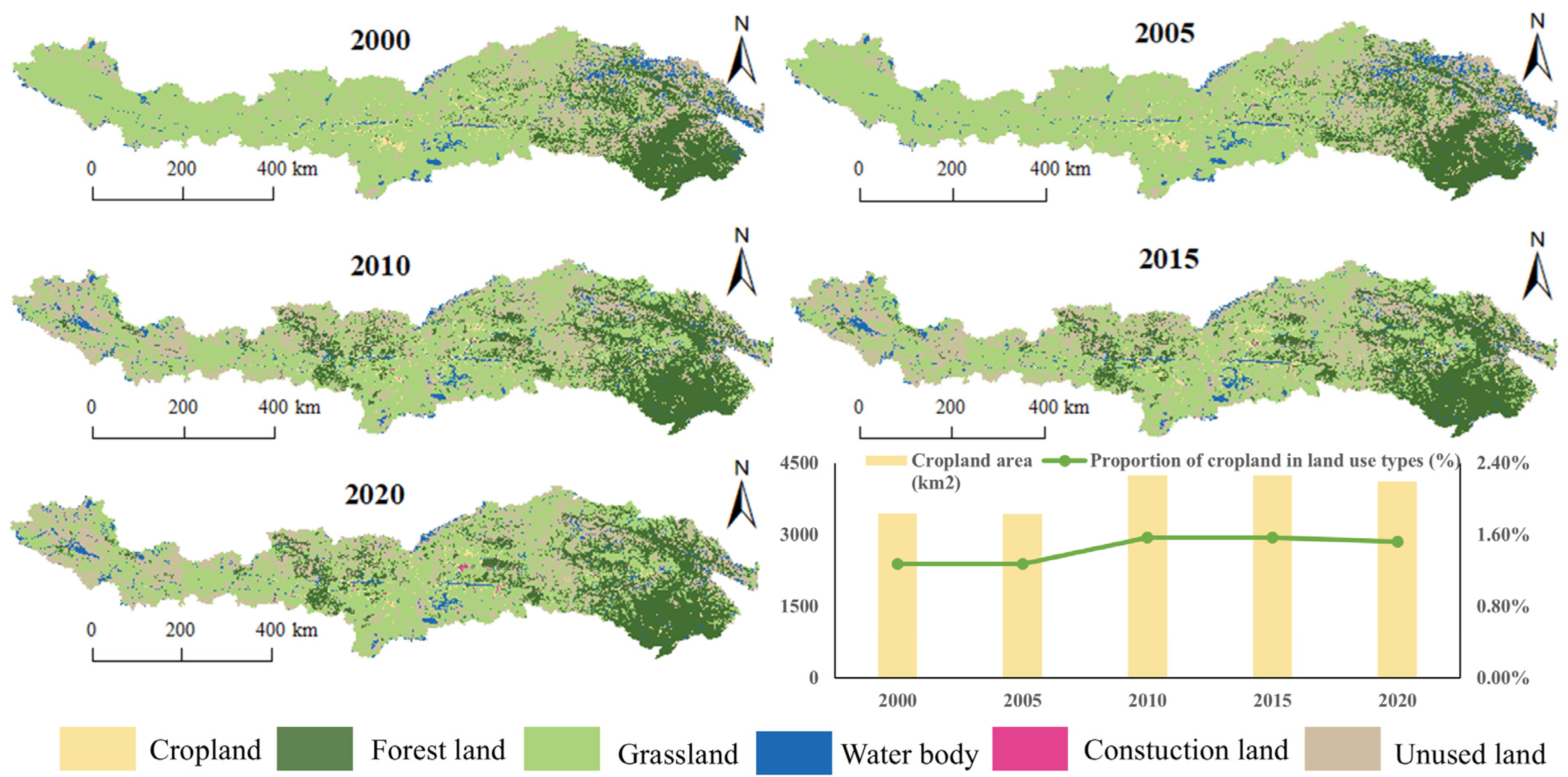
3.1. Characteristics of Land Use Type Changes
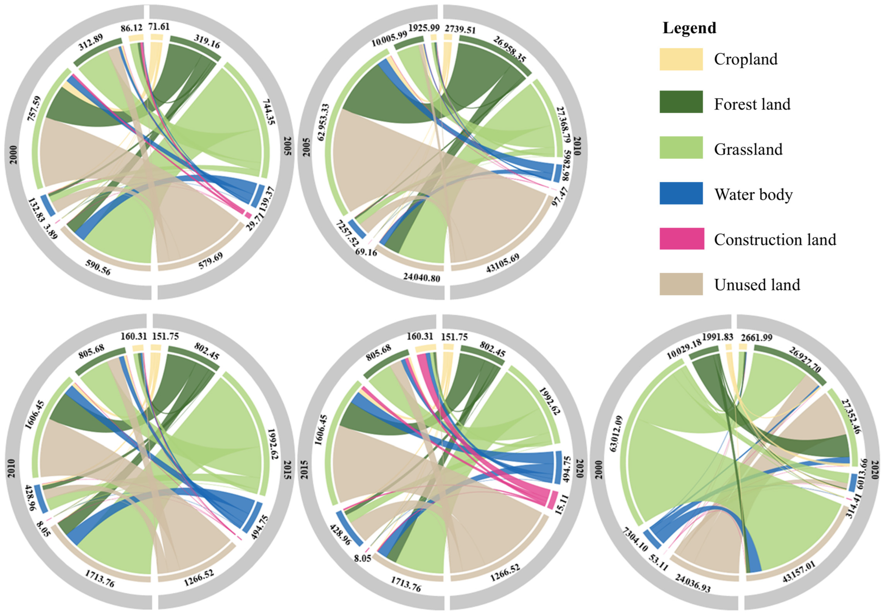
3.2. Land Use Transition Matrix Analysis
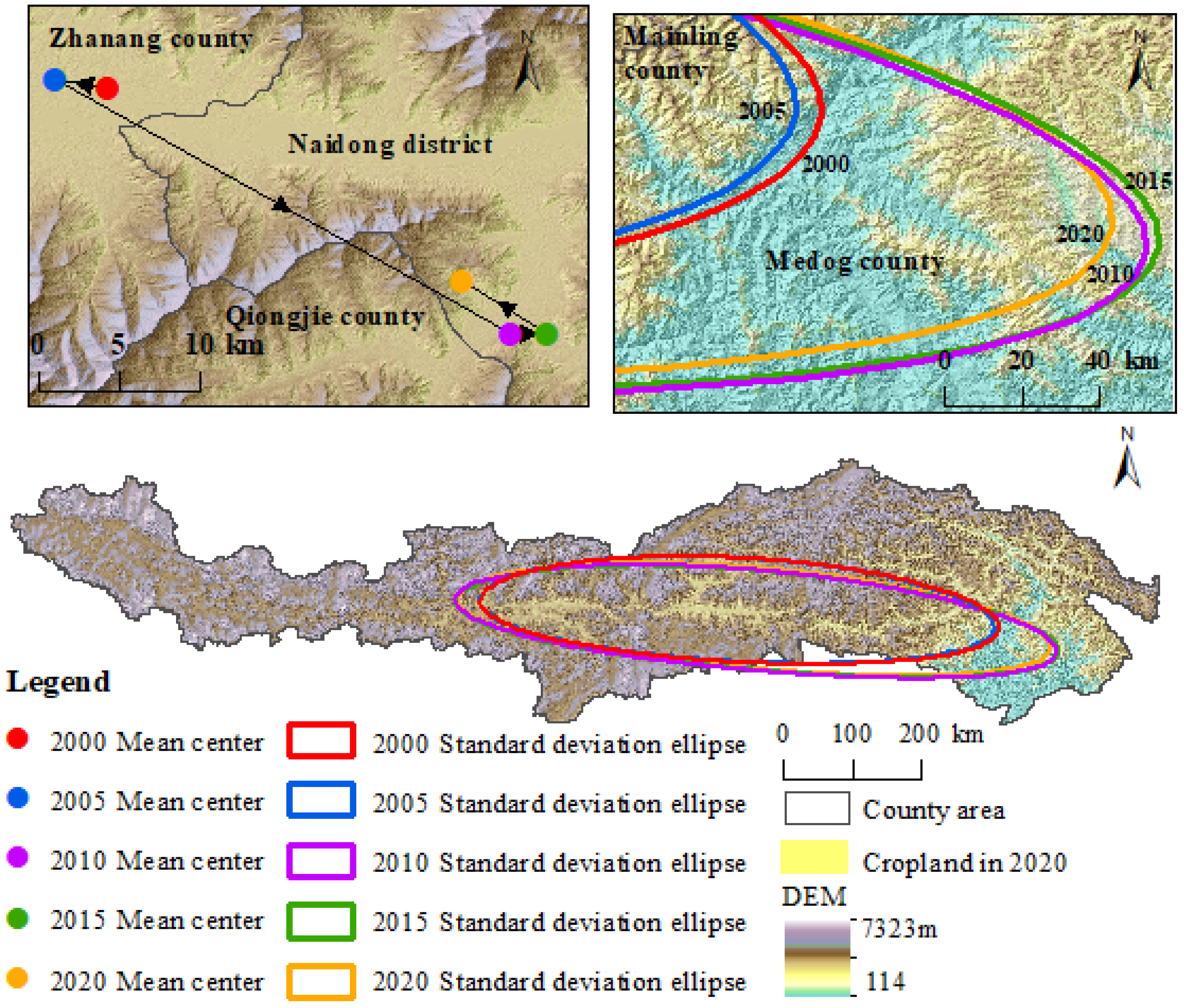
3.3. Center of Gravity Shift and Standard Deviation Ellipse
3.4. Cropland Change Driving Force Analysis
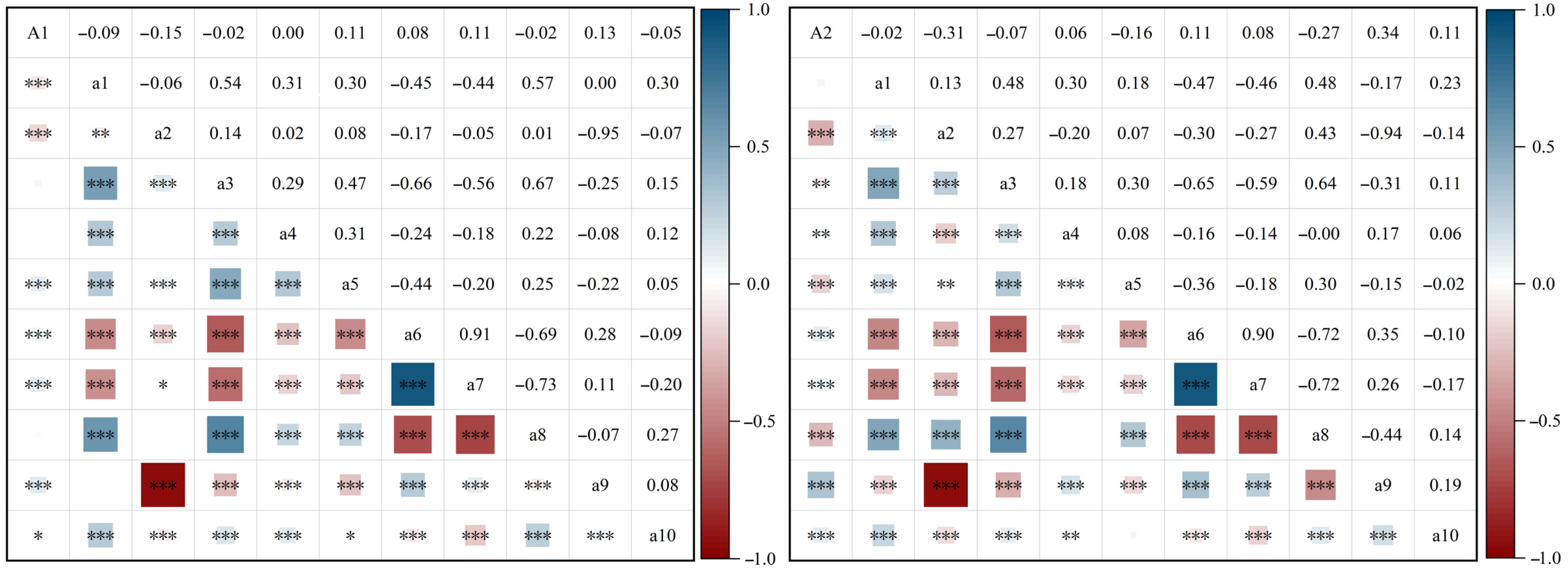
3.4.1. Correlation Analysis Between Driving Factors and Cropland Area
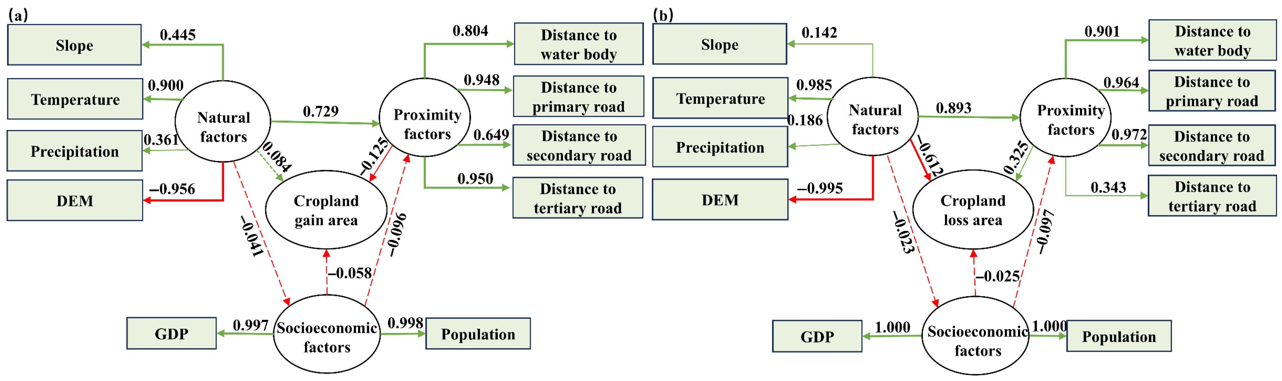
3.4.2. Analysis of Driving Factors Based on PLS-SEM
- (1)
- Natural factors, socioeconomic factors, and proximity factors directly influence changes in cropland area;
- (2)
- Natural factors indirectly influence cropland area changes through their impact on proximity and socioeconomic factors;
- (3)
- Socioeconomic factors indirectly influence cropland area changes through their effect on proximity factors.
3.4.3. Impact of Latent and Manifest Variables on Cropland Area Change
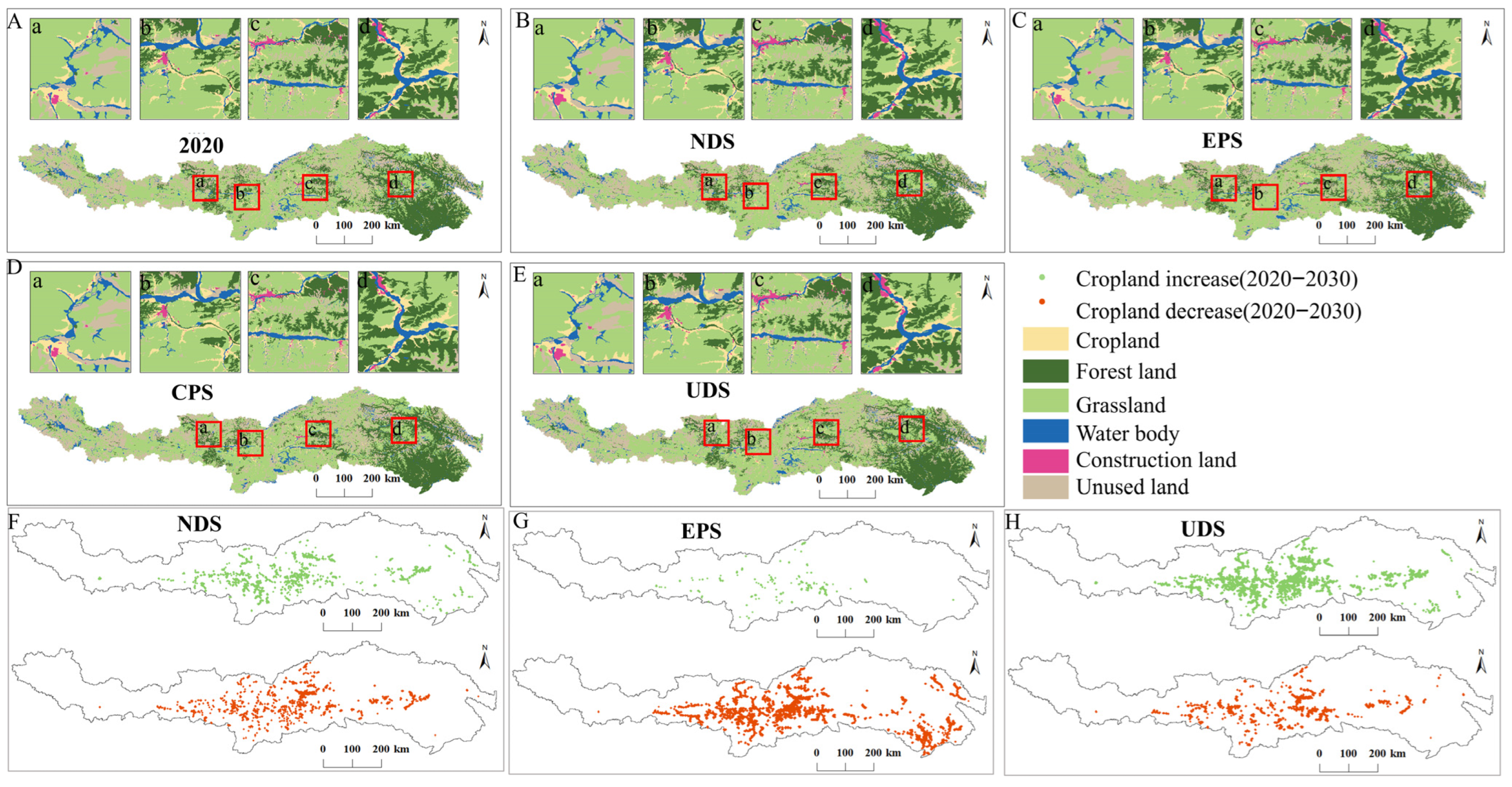
3.5. Cropland Landscape Distribution in 2030 Under Different Scenarios
3.5.1. Natural Development Scenario (NDS)
3.5.2. Cropland Protection Scenario (CPS)
3.5.3. Ecological Protection Scenario (EPS)
3.5.4. Urban Development Scenario (UDS)
4. Discussion and Conclusions
4.1. Discussion
4.1.1. Spatiotemporal Dynamics of Cropland
4.1.2. Factors Driving Cropland Area Changes
4.1.3. Multi-Scenario Simulation of Cropland in 2030
4.1.4. Limitations of the Study
4.2. Conclusions
- (1)
- Cropland in the YZRB showed a fluctuating but overall increasing trend from 2000 to 2020, primarily driven by the conversion of forest and grassland into cropland. Although some cropland was lost to forest, grassland, and water bodies, the net gain resulted in a dynamic degree of 0.97%, reflecting continued expansion.
- (2)
- The spatial distribution of cropland shifted significantly, with the centroid migrating northwest (2000–2005), southeast (2005–2015), and back northwest (2015–2020). A consistent northwest–southeast pattern was observed, shaped by topography and climate. Changes in the standard deviational ellipse indicated initial concentration and later dispersion of cropland, aligning with the expansion pattern.
- (3)
- Spatiotemporal changes in cropland were jointly driven by natural and socioeconomic factors, as confirmed by robust PLS-SEM model validation (Q2 > 0, AVE > 0.5, GOF > 0.36). Natural factors had a direct positive influence on cropland increase and mediated the impacts of socioeconomic and distance variables, which mainly exerted negative effects.
- (4)
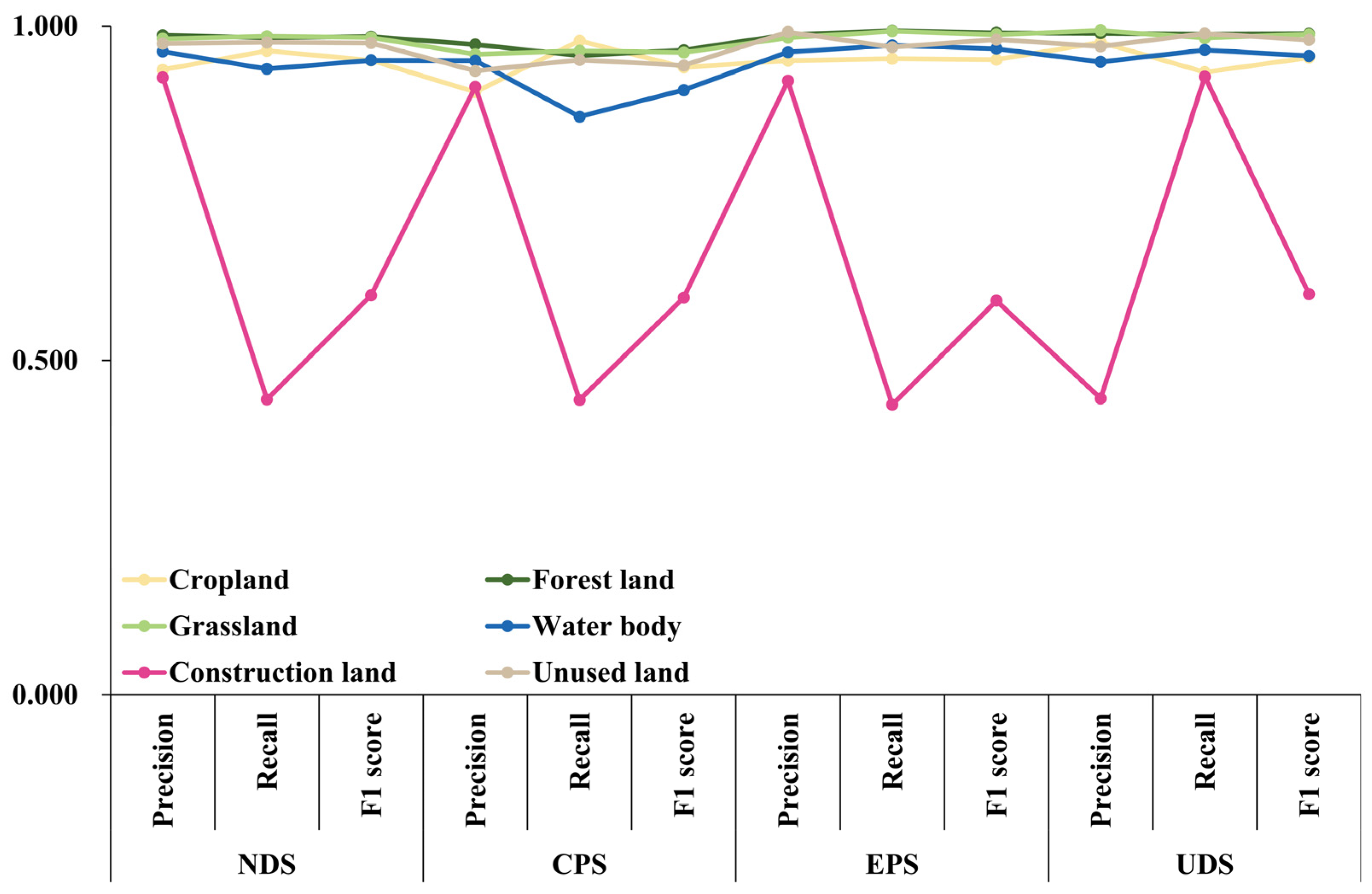
- The PLUS model accurately simulated land use in 2020 and projected divergent outcomes for 2030 under different policy scenarios. Cropland declined most in the Natural Development and Ecological Protection scenarios, remained relatively stable in the Cropland Protection scenario, and experienced significant losses under Urban Development due to rapid urban expansion.
Author Contributions
Funding
Data Availability Statement
Conflicts of Interest
References
- Su, Y.; Qian, K.; Lin, L.; Wang, K.; Guan, T.; Gan, M. Identifying the driving forces of non-grain production expansion in rural China and its implications for policies on cultivated land protection. Land Use Policy 2020, 92, 104435. [Google Scholar] [CrossRef]
- Zhou, Y.; Li, X.; Liu, Y. Cultivated land protection and rational use in China. Land Use Policy 2021, 106, 105454. [Google Scholar] [CrossRef]
- Foley, J.A.; Ramankutty, N.; Brauman, K.A.; Cassidy, E.S.; Gerber, J.S.; Johnston, M.; Mueller, N.D.; O’Connell, C.; Ray, D.K.; West, P.C.; et al. Solutions for a cultivated planet. Nature 2011, 478, 337–342. [Google Scholar] [CrossRef] [PubMed]
- Godfray, H.C.; Beddington, J.R.; Crute, I.R.; Haddad, L.; Lawrence, D.; Muir, J.F.; Pretty, J.; Robinson, S.; Thomas, S.M.; Toulmin, C. Food security: The challenge of feeding 9 billion people. Science 2010, 327, 812–818. [Google Scholar] [CrossRef]
- Prăvălie, R.; Patriche, C.; Borrelli, P.; Panagos, P.; Roșca, B.; Dumitraşcu, M.; Nita, I.-A.; Săvulescu, I.; Birsan, M.-V.; Bandoc, G. Arable lands under the pressure of multiple land degradation processes. A global perspective. Environ. Res. 2021, 194, 110697. [Google Scholar] [CrossRef]
- Zhang, T.; Cheng, C.; Shen, S.; Yang, Y.; Ye, S. Coupled impact of climate change and human activities on farmland loss on the Tibetan Plateau. Land Use Policy 2025, 154, 107558. [Google Scholar] [CrossRef]
- Wang, Y.; Li, X.; Xin, L.; Tan, M. Farmland marginalization and its drivers in mountainous areas of China. Sci. Total Environ. 2020, 719, 135132. [Google Scholar] [CrossRef]
- Wang, A.; Tao, H.; Ding, G.; Zhang, B.; Huang, J.; Wu, Q. Global cropland exposure to extreme compound drought heatwave events under future climate change. Weather. Clim. Extrem. 2023, 40, 100559. [Google Scholar] [CrossRef]
- Cheng, H.; Wang, X.; Chen, D. Research on Spatial–Temporal Variations of Cultivated Land in China Based on GlobeLand30. Front. Environ. Sci. 2022, 10, 929760. [Google Scholar] [CrossRef]
- Li, X.; Zhang, X.; Jin, X. Spatio–temporal characteristics and driving factors of cultivated land change in various agricultural regions of China: A detailed analysis based on County-level data. Ecol. Indic. 2024, 166, 112485. [Google Scholar] [CrossRef]
- Liu, Y.; Liu, S.; Sun, Y.; Wang, F.; Li, M. Driving forces of cultivated land evolution in agro-pastoral areas on the Qinghai-Tibet Plateau based on ecological niche theory. J. Clean. Prod. 2021, 313, 127899. [Google Scholar] [CrossRef]
- Xiao, Y.; Wang, J.; Wang, B.; Fan, B.; Zhou, G. Soil microbial network complexity predicts soil multifunctionality better than soil microbial diversity during grassland–farmland–shrubland conversion on the Qinghai-Tibetan Plateau. Agric. Ecosyst. Environ. 2025, 379, 109356. [Google Scholar] [CrossRef]
- Haddaway, N.R.; Styles, D.; Pullin, A.S. Evidence on the environmental impacts of farm land abandonment in high altitude/mountain regions: A systematic map. Environ. Evid. 2014, 3, 17. [Google Scholar] [CrossRef]
- Zhu, Z.; Qiu, S.; Ye, S. Remote sensing of land change: A multifaceted perspective. Remote Sens. Environ. 2022, 282, 113266. [Google Scholar] [CrossRef]
- Valjarević, A.; Morar, C.; Brasanac-Bosanac, L.; Cirkovic-Mitrovic, T.; Djekic, T.; Mihajlović, M.; Milevski, I.; Culafic, G.; Luković, M.; Niemets, L.; et al. Sustainable land use in Moldova: GIS & remote sensing of forests and crops. Land Use Policy 2025, 152, 107515. [Google Scholar] [CrossRef]
- Lange, S.; Müller, F. Geographic Information Systems (GIS) and Terrestrial Ecosystems. In Reference Module in Earth Systems and Environmental Sciences; Elsevier: Amsterdam, The Netherlands, 2024. [Google Scholar]
- Duan, X.; Haseeb, M.; Tahir, Z.; Mahmood, S.A.; Tariq, A. Analyzing and predicting land use and land cover dynamics using multispectral high-resolution imagery and hybrid CA-Markov modeling. Land Use Policy 2025, 157, 107655. [Google Scholar] [CrossRef]
- He, Y.; Wu, W.; Xie, X.; Ke, X.; Song, Y.; Zhou, C.; Li, W.; Li, Y.; Jing, R.; Song, P.; et al. Land Use/Cover Change Prediction Based on a New Hybrid Logistic–Multicriteria Evaluation–Cellular Automata–Markov Model Taking Hefei, China as an Example. Land 2023, 12, 1899. [Google Scholar] [CrossRef]
- Luo, G.; Yin, C.; Chen, X.; Xu, W.; Lu, L. Combining system dynamic model and CLUE–S model to improve land use scenario analyses at regional scale: A case study of Sangong watershed in Xinjiang, China. Ecol. Complex. 2010, 7, 198–207. [Google Scholar] [CrossRef]
- Lin, Z.; Peng, S. Comparison of multimodel simulations of land use and land cover change considering integrated constraints—A case study of the Fuxian Lake basin. Ecol. Indic. 2022, 142, 109254. [Google Scholar] [CrossRef]
- Liu, X.; Liang, X.; Li, X.; Xu, X.; Ou, J.; Chen, Y.; Li, S.; Wang, S.; Pei, F. A future land use simulation model (FLUS) for simulating multiple land use scenarios by coupling human and natural effects. Landsc. Urban Plan. 2017, 168, 94–116. [Google Scholar] [CrossRef]
- Zhang, Y.; Yu, P.; Tian, Y.; Chen, H.; Chen, Y. Exploring the impact of integrated spatial function zones on land use dynamics and ecosystem services tradeoffs based on a future land use simulation (FLUS) model. Ecol. Indic. 2023, 150, 110246. [Google Scholar] [CrossRef]
- Zhang, Z.; Hu, B.; Jiang, W.; Qiu, H. Spatial and temporal variation and prediction of ecological carrying capacity based on machine learning and PLUS model. Ecol. Indic. 2023, 154, 110611. [Google Scholar] [CrossRef]
- Zhang, J.; Cao, P.; Roosli, R. Assessing land use and carbon storage changes using PLUS and InVEST models: A multi-scenario simulation in Hohhot. Environ. Sustain. Indic. 2025, 26, 100655. [Google Scholar] [CrossRef]
- Shi, J.; Zhang, P.; Liu, Y.; Tian, L.; Cao, Y.; Guo, Y.; Li, J.; Wang, Y.; Huang, J.; Jin, R.; et al. Study on spatiotemporal changes of wetlands based on PLS-SEM and PLUS model: The case of the Sanjiang Plain. Ecol. Indic. 2024, 169, 112812. [Google Scholar] [CrossRef]
- Wang, C.; Ma, L.; Zhang, Y.; Chen, N.; Wang, W. Spatiotemporal dynamics of wetlands and their driving factors based on PLS-SEM: A case study in Wuhan. Sci. Total Environ. 2022, 806, 151310. [Google Scholar] [CrossRef]
- Li, F.; Xu, Z.; Feng, Y.; Liu, M.; Liu, W. Changes of land cover in the Yarlung Tsangpo River basin from 1985 to 2005. Environ. Earth Sci. 2013, 68, 181–188. [Google Scholar] [CrossRef]
- Huang, X.; Wang, Y.; Wang, X.; Chen, J.; Ma, J.; Liang, E.; Wang, X. Exploring the natural–socioeconomic driving and response mechanisms of ecosystem services interactions to optimize ecosystem management: A case study in the Yarlung Zangbo River Basin. Sci. Total Environ. 2024, 957, 177842. [Google Scholar] [CrossRef]
- Gu, H.; Xu, Y.-P.; Wang, L.; Ma, D.; Liang, X.; Guo, Y.; Liu, L. Seasonal streamflow forecasting by surrogate modeling in the Yarlung Zangbo River Basin, China. J. Hydrol. Reg. Stud. 2024, 53, 101835. [Google Scholar] [CrossRef]
- Li, C.; Hao, J.; Zhang, G.; Fang, H.; Wang, Y.; Lu, H. Runoff variations affected by climate change and human activities in Yarlung Zangbo River, southeastern Tibetan Plateau. CATENA 2023, 230, 107184. [Google Scholar] [CrossRef]
- Li, D.; Chen, G.; Xi, Z.; He, P.; Xin, X.; Chen, J.; Yu, H.; Kang, G. Spatiotemporal changes of cultivated land utilization in black soil region, China based on geo–information Tupu. Sci. Rep. 2025, 15, 10306. [Google Scholar] [CrossRef]
- Yang, G.; Wang, H.; Wang, L.; Shao, W. Analysis of the relationship between food production, water resources and power consumption in North China. Energy Procedia 2017, 142, 2574–2579. [Google Scholar] [CrossRef]
- Guo, N.; Shi, X.; Zhao, Y.; Xu, S.; Wang, M.; Zhang, G.; Wu, J.; Huang, B.; Kong, C. Environmental and Anthropogenic Factors Driving Changes in Paddy Soil Organic Matter: A Case Study in the Middle and Lower Yangtze River Plain of China. Pedosphere 2017, 27, 926–937. [Google Scholar] [CrossRef]
- Shen, W.; Li, H.; Sun, M.; Jiang, J. Dynamics of aeolian sandy land in the Yarlung Zangbo River basin of Tibet, China from 1975 to 2008. Glob. Planet. Change 2012, 86–87, 37–44. [Google Scholar] [CrossRef]
- Zhou, H.; Tang, M.; Huang, J.; Mei, X.; Zhao, H. Driving mechanisms and multi-scenario simulation of land use change based on National Land Survey Data: A case in Jianghan Plain, China. Front. Environ. Sci. 2024, 12, 1422987. [Google Scholar] [CrossRef]
- Wang, X.; Bao, Y. Study on the methods of land use dynamic change research. Prog. Geogr. 1999, 18, 83–89. [Google Scholar] [CrossRef]
- Ye, G.; Chen, K.; Yang, Y.; Liang, S.; Hu, W.; He, L. Integrative Framework for Decoding Spatial and Temporal Drivers of Land Use Change in Malaysia: Strategic Insights for Sustainable Land Management. Land 2024, 13, 2248. [Google Scholar] [CrossRef]
- Grether, J.-M.; Mathys, N. Is the World’s Economic Centre of Gravity Already in Asia? Area 2010, 42, 47–50. [Google Scholar] [CrossRef]
- Wang, J.; You, K.; Qi, L.; Ren, H. Gravity center change of carbon emissions in Chinese residential building sector: Differences between urban and rural area. Energy Rep. 2022, 8, 10644–10656. [Google Scholar] [CrossRef]
- Wang, S.; Qin, C.; Zhao, Y.; Zhao, J.; Han, Y. The Evolutionary Path of the Center of Gravity for Water Use, the Population, and the Economy, and Their Decomposed Contributions in China from 1965 to 2019. Sustainability 2023, 15, 9275. [Google Scholar] [CrossRef]
- Chen, P.; Duan, J.; Wang, Y. Spatio–temporal evolution and driving forces of urban gravity centers and ecological security risk gravity centers in China. Ecol. Indic. 2025, 170, 113025. [Google Scholar] [CrossRef]
- Shi, Y.; Matsunaga, T.; Yamaguchi, Y.; Zhao, A.; Li, Z.; Gu, X. Long-term trends and spatial patterns of PM2.5–induced premature mortality in South and Southeast Asia from 1999 to 2014. Sci. Total Environ. 2018, 631–632, 1504–1514. [Google Scholar] [CrossRef] [PubMed]
- Cai, H.; Yu, J.; Guo, Y. Spatial and temporal distribution and evolution of traditional villages in Xin ’an River Basin of China based on geographic detection and remote sensing technology. Ecol. Indic. 2025, 171, 113239. [Google Scholar] [CrossRef]
- Duman, Z.; Mao, X.; Cai, B.; Zhang, Q.; Chen, Y.; Gao, Y.; Guo, Z. Exploring the spatiotemporal pattern evolution of carbon emissions and air pollution in Chinese cities. J. Environ. Manag. 2023, 345, 118870. [Google Scholar] [CrossRef]
- Sander, T.; Teh, P. SmartPLS for the Human Resources Field To Evaluate a Model. In New Challenges of Economic and Business Development; University of Latvia: Riga, Latvia, 2014. [Google Scholar]
- Sarstedt, M.; Cheah, J.-H. Partial least squares structural equation modeling using SmartPLS: A software review. J. Mark. Anal. 2019, 7, 196–202. [Google Scholar] [CrossRef]
- Liu, C.; Zhang, F.; Jim, C.-Y.; Johnson, V.C.; Tan, M.L.; Shi, J.; Lin, X. Controlled and driving mechanism of the SPM variation of shallow Brackish Lakes in arid regions. Sci. Total Environ. 2023, 878, 163127. [Google Scholar] [CrossRef] [PubMed]
- Liang, X.; Guan, Q.; Clarke, K.C.; Liu, S.; Wang, B.; Yao, Y. Understanding the drivers of sustainable land expansion using a patch-generating land use simulation (PLUS) model: A case study in Wuhan, China. Comput. Environ. Urban Syst. 2021, 85, 101569. [Google Scholar] [CrossRef]
- Guo, A.; Zhang, Y.; Hao, Q. Monitoring and Simulation of Dynamic Spatiotemporal Land Use/Cover Changes. Complexity 2020, 2020, 3547323. [Google Scholar] [CrossRef]
- Wang, Q.; Bai, X.; Zhang, D.; Wang, H. Spatiotemporal characteristics and multi-scenario simulation of land use change and ecological security in the mountainous areas: Implications for supporting sustainable land management and ecological planning. Sustain. Futures 2024, 8, 100286. [Google Scholar] [CrossRef]
- Wang, Z.; Li, Z.; Liu, X.; Song, H.; Liu, S.; Qi, J.; Jing, F.; Gao, Z. Ecological analysis and multi-scenario simulation of Yellow River Delta wetland under clearing of Spartina alterniflora. Glob. Ecol. Conserv. 2024, 56, e03287. [Google Scholar] [CrossRef]
- Wu, Q.; Wang, L.; Wang, T.; Ruan, Z.; Du, P. Spatial–temporal evolution analysis of multi-scenario land use and carbon storage based on PLUS–InVEST model: A case study in Dalian, China. Ecol. Indic. 2024, 166, 112448. [Google Scholar] [CrossRef]
- Li, W.; Kang, J.; Wang, Y. Identifying the contribution and spatial effects of land use conversion on ecosystem health in Chongqing: A multi-scenario simulation perspective. Ecol. Indic. 2024, 165, 112232. [Google Scholar] [CrossRef]
- Xu, C.; Zhang, Q.; Yu, Q.; Wang, J.; Wang, F.; Qiu, S.; Ai, M.; Zhao, J. Effects of land use/cover change on carbon storage between 2000 and 2040 in the Yellow River Basin, China. Ecol. Indic. 2023, 151, 110345. [Google Scholar] [CrossRef]
- Liu, J.; Liu, B.; Wu, L.; Miao, H.; Liu, J.; Jiang, K.; Ding, H.; Gao, W.; Liu, T. Prediction of land use for the next 30 years using the PLUS model’s multi-scenario simulation in Guizhou Province, China. Sci. Rep. 2024, 14, 13143. [Google Scholar] [CrossRef]
- Zhang, C.; Jia, Q.; Liu, Y.; Zheng, Z.; Gao, Y.; Li, K. Evaluation and multi scenario simulation of ecosystem service value in Zhengzhou Metropolitan Area based on PLUS model. Meas. Sens. 2024, 32, 101079. [Google Scholar] [CrossRef]
- Lin, X.; Fu, H. Multi-scenario simulation analysis of cultivated land based on PLUS model—A case study of Haikou, China. Front. Ecol. Evol. 2023, 11, 1197419. [Google Scholar] [CrossRef]
- Xu, B.; Li, J.; Liu, Y.; Zhang, T.; Luo, Z.; Pei, X. Disentangling the response of vegetation dynamics to natural and anthropogenic drivers over the Qinghai-Tibet Plateau using dimensionality reduction and structural equation model. For. Ecol. Manag. 2024, 554, 121677. [Google Scholar] [CrossRef]
- Gu, Z.; Chen, X.; Ruan, W.; Zheng, M.; Gen, K.; Li, X.; Deng, H.; Chen, Y.; Liu, M. Quantifying the direct and indirect effects of terrain, climate and human activity on the spatial pattern of kNDVI–based vegetation growth: A case study from the Minjiang River Basin, Southeast China. Ecol. Inform. 2024, 80, 102493. [Google Scholar] [CrossRef]
- Li, C.; Yang, M.; Li, Z.; Wang, B. How Will Rwandan Land Use/Land Cover Change under High Population Pressure and Changing Climate? Appl. Sci. 2021, 11, 5376. [Google Scholar] [CrossRef]
- Liu, Y.; Jing, Y.; Han, S. Multi-scenario simulation of land use/land cover change and water yield evaluation coupled with the GMOP–PLUS–InVEST model: A case study of the Nansi Lake Basin in China. Ecol. Indic. 2023, 155, 110926. [Google Scholar] [CrossRef]
- Zhai, H.; Lv, C.; Liu, W.; Yang, C.; Fan, D.; Wang, Z.; Guan, Q. Understanding Spatio–Temporal Patterns of Land Use/Land Cover Change under Urbanization in Wuhan, China, 2000–2019. Remote Sens. 2021, 13, 3331. [Google Scholar] [CrossRef]
- Zhang, J.; Wang, J.; Chen, Y.; Huang, S.; Liang, B. Spatiotemporal variation and prediction of NPP in Beijing–Tianjin–Hebei region by coupling PLUS and CASA models. Ecol. Inform. 2024, 81, 102620. [Google Scholar] [CrossRef]
- Chen, L.; Cai, H. Study on land use conflict identification and territorial spatial zoning control in Rao River Basin, Jiangxi Province, China. Ecol. Indic. 2022, 145, 109594. [Google Scholar] [CrossRef]
- Demessie, S.F.; Dile, Y.T.; Bedadi, B.; Tarkegn, T.G.; Bayabil, H.K.; Sintayehu, D.W. Assessing and projecting land use land cover changes using machine learning models in the Guder watershed, Ethiopia. Environ. Chall. 2025, 18, 101074. [Google Scholar] [CrossRef]
- Zeng, J.; Luo, T.; Gu, T.; Chen, W. How does cultivated land fragmentation affect soil erosion: Evidence from the Yangtze River Basin in China. J. Environ. Manag. 2024, 360, 121020. [Google Scholar] [CrossRef]
- Huang, X.; Wang, H.; Xiao, F. Simulating urban growth affected by national and regional land use policies: Case study from Wuhan, China. Land Use Policy 2022, 112, 105850. [Google Scholar] [CrossRef]
- Wei, Q.; Abudureheman, M.; Halike, A.; Yao, K.; Yao, L.; Tang, H.; Tuheti, B. Temporal and spatial variation analysis of habitat quality on the PLUS–InVEST model for Ebinur Lake Basin, China. Ecol. Indic. 2022, 145, 109632. [Google Scholar] [CrossRef]
- Wu, J.; Luo, J.; Zhang, H.; Qin, S.; Yu, M. Projections of land use change and habitat quality assessment by coupling climate change and development patterns. Sci. Total Environ. 2022, 847, 157491. [Google Scholar] [CrossRef]
- Loukika, K.N.; Keesara, V.R.; Buri, E.S.; Sridhar, V.; Dzwairo, B.; Montenegro, S. Integrated impacts of land use changes and climate dynamics on hydrological components in the Munneru River basin, India. J. Environ. Manag. 2025, 380, 125096. [Google Scholar] [CrossRef]
- Wang, X.; Wang, D.; Wu, S.; Yan, Z.; Han, J. Cultivated land multifunctionality in undeveloped peri–urban agriculture areas in China: Implications for sustainable land management. J. Environ. Manag. 2023, 325, 116500. [Google Scholar] [CrossRef]
- Li, S.; Pu, J.; Deng, X. Agricultural land use transition under multidimensional topographical gradients and its impact on ecosystem service interactions. J. Integr. Agric. 2025, in press. [Google Scholar]
- Tarolli, P.; Straffelini, E. Agriculture in Hilly and Mountainous Landscapes: Threats, Monitoring and Sustainable Management. Geogr. Sustain. 2020, 1, 70–76. [Google Scholar] [CrossRef]
- Seydehmet, J.; Zhou, X.; Chen, H.; Wang, Y. The spatiotemporal evaluation of ecosystem stability by simulating land use change in edge oasis of the Tarim basin, northwest China. Heliyon 2025, e42621. [Google Scholar] [CrossRef]
- Bren d’Amour, C.; Reitsma, F.; Baiocchi, G.; Barthel, S.; Güneralp, B.; Erb, K.H.; Haberl, H.; Creutzig, F.; Seto, K.C. Future urban land expansion and implications for global croplands. Proc. Natl. Acad. Sci. USA 2017, 114, 8939–8944. [Google Scholar] [CrossRef]
- Ibraeva, A.; Correia, G.H.d.A.; Silva, C.; Antunes, A.P. Transit–oriented development: A review of research achievements and challenges. Transp. Res. Part A Policy Pract. 2020, 132, 110–130. [Google Scholar] [CrossRef]
- Tong, X.; Wang, Y.; Chan, E.H.W.; Zhou, Q. Correlation between Transit–Oriented Development (TOD), Land Use Catchment Areas, and Local Environmental Transformation. Sustainability 2018, 10, 4622. [Google Scholar] [CrossRef]
- Zhou, J.; Johnson, V.C.; Shi, J.; Tan, M.L.; Zhang, F. Multi-scenario land use change simulation and spatial–temporal evolution of carbon storage in the Yangtze River Delta region based on the PLUS–InVEST model. PLoS ONE 2025, 20, e0316255. [Google Scholar] [CrossRef]
- Shi, X.; Wang, W.; Shi, W. Progress on quantitative assessment of the impacts of climate change and human activities on cropland change. J. Geogr. Sci. 2016, 26, 339–354. [Google Scholar] [CrossRef]

| Type | Data | Data Sources | Original Resolution | Year |
|---|---|---|---|---|
| Land use data | Land use classification data of the study area | Resource and Environmental Science and Data Center, Chinese Academy of Sciences (https://www.resdc.cn) (accessed on 14 August 2024) | 30 m | 2000, 2005, 2010, 2015, and 2020 |
| Permanent basic farmland | The Department of Natural Resources of the Tibet Autonomous Region (accessed on 13 April 2025) | 2020 | ||
| Ecological red line | ||||
| Nature reserve | ||||
| Socioeconomic data | Population | Resource and Environmental Science and Data Center, Chinese Academy of Sciences (https://www.resdc.cn) (accessed on 13 September 2024) | 1000 m | |
| GDP | ||||
| Climate and environmental data | Temperature | |||
| Precipitation | ||||
| DEM | Geospatial Data Cloud (accessed on 13 September 2024) | 30 m | ||
| Slope | ||||
| Distance to water body | OpenStreetMap (https://www.openstreetmap.org/) (accessed on 13 September 2024) | |||
| Proximity data | Distance to primary road | Resource and Environmental Science and Data Center, Chinese Academy of Sciences (https://www.resdc.cn) (accessed on 14 August 2024) | 1000 m | |
| Distance to secondary road | ||||
| Distance to tertiary road |
| Land Use Type | NDS | CPS | EPS | UDS | ||||||||||||||||||||
|---|---|---|---|---|---|---|---|---|---|---|---|---|---|---|---|---|---|---|---|---|---|---|---|---|
| a | b | c | d | e | f | a | b | c | d | e | f | a | b | c | d | e | f | a | b | c | d | e | f | |
| a | 1 | 0 | 1 | 0 | 1 | 1 | 1 | 0 | 0 | 0 | 0 | 0 | 1 | 1 | 1 | 1 | 1 | 1 | 1 | 0 | 0 | 0 | 1 | 1 |
| b | 0 | 1 | 1 | 0 | 0 | 1 | 1 | 1 | 1 | 0 | 0 | 1 | 0 | 1 | 0 | 0 | 0 | 0 | 1 | 1 | 0 | 0 | 1 | 1 |
| c | 1 | 1 | 1 | 1 | 1 | 1 | 1 | 1 | 1 | 1 | 1 | 1 | 0 | 1 | 1 | 1 | 0 | 0 | 1 | 0 | 1 | 0 | 1 | 0 |
| d | 1 | 0 | 1 | 1 | 0 | 1 | 1 | 0 | 1 | 1 | 0 | 1 | 0 | 0 | 0 | 1 | 0 | 0 | 0 | 1 | 1 | 1 | 1 | 0 |
| e | 0 | 0 | 0 | 0 | 1 | 0 | 0 | 0 | 0 | 0 | 1 | 0 | 0 | 0 | 0 | 0 | 1 | 0 | 0 | 1 | 1 | 0 | 1 | 0 |
| F | 1 | 1 | 1 | 1 | 1 | 1 | 1 | 1 | 1 | 1 | 1 | 1 | 1 | 1 | 1 | 1 | 1 | 1 | 1 | 1 | 1 | 1 | 1 | 1 |
| Type | Cropland | Forest Land | Grassland | Water Body | Construction Land | Unused Land |
|---|---|---|---|---|---|---|
| NDS | 0.551 | 0.220 | 0.221 | 0.100 | 1.000 | 0.243 |
| CPS | 0.370 | 0.328 | 0.315 | 0.100 | 1.000 | 0.458 |
| EPS | 0.722 | 0.327 | 1.000 | 0.100 | 0.983 | 0.412 |
| UDS | 0.535 | 0.212 | 0.221 | 0.100 | 1.000 | 0.180 |
| Land Use Type | Year | Single Dynamic Degree/% | ||||
|---|---|---|---|---|---|---|
| 2000 | 2005 | 2010 | 2015 | 2020 | 2000–2020 | |
| Cropland | 3449.51 | 3437.27 | 4250.71 | 4242.88 | 4121.81 | 0.97 |
| Forest land | 45,684.47 | 45,691.02 | 62,680.46 | 62,665.45 | 62,621.18 | –3.05 |
| Grassland | 160,398.80 | 160,374.80 | 124,851.60 | 125,230.90 | 124,791.20 | –1.11 |
| Water body | 12,268.27 | 12,277.18 | 11,117.16 | 11,178.81 | 11,096.12 | –0.48 |
| Construction land | 118.17 | 144.38 | 172.31 | 179.63 | 379.47 | 11.06 |
| Unused land | 48,136.84 | 48,133.11 | 67,321.30 | 66,869.17 | 67,386.88 | 2.00 |
| Year | 2000 | 2005 | 2010 | 2015 | 2020 |
|---|---|---|---|---|---|
| Major Axis Standard Deviation (km) | 326.67 | 323.77 | 380.83 | 381.59 | 375.46 |
| Minor Axis Standard Deviation (km) | 76.22 | 75.86 | 73.28 | 72.43 | 73.66 |
| Rotation Angle (°) | 101.38 | 101.41 | 103.59 | 103.35 | 103.24 |
| Area (km2) | 78,194.28 | 77,133.50 | 87,631.46 | 86,797.27 | 86,843.72 |
| Perimeter (km) | 1390.99 | 1379.24 | 1595.08 | 1596.68 | 1574.91 |
| Flattening | 0.77 | 0.77 | 0.81 | 0.81 | 0.80 |
| Model Performance Indicators | Type | Value (Cropland Increase) | Value (Cropland Decrease) | Standard | Description |
|---|---|---|---|---|---|
| R2 | Socioeconomic factors | 0.001 | 0.000 | >0.67 | Substantial explanatory power |
| Proximity factors | 0.546 | 0.811 | >0.33 | Moderate explanatory power | |
| / | / | / | >0.19 | Weak explanatory power | |
| Q2 | Socioeconomic factors | 0.002 | 0.001 | >0 | A larger value denoting higher prediction accuracy of the model |
| Natural factors | 0.000 | 0.000 | |||
| Proximity factors | 0.373 | 0.554 | |||
| AVE | Socioeconomic factors | 0.995 | 0.999 | >0.5 | A higher value indicates better convergent validity of the model |
| Natural factors | 0.513 | 0.503 | |||
| Proximity factors | 0.717 | 0.701 | |||
| p–value | Socioeconomic factors-Cropland | 0.000 *** | 0.000 *** | ≤0.001 | Statistically significant |
| Natural factors-Cropland | 0.001 ** | 0.000 *** | |||
| Proximity factors-Cropland | 0.000 *** | 0.000 *** | |||
| GOF | / | 0.385 | 0.486 | 0.1 | Weak model fitting |
| / | 0.25 | Medium model fitting | |||
| / | 0.36 | Strong model fitting |
| Type | 2020 | NDS | CPS | EPS | UDS | ||||
|---|---|---|---|---|---|---|---|---|---|
| Area | Area | CR (%) | Area | CR (%) | Area | CR (%) | Area | CR (%) | |
| Cropland | 4121.81 | 4002.92 | −2.88 | 4121.42 | −0.01 | 4002.92 | −2.88 | 4006.15 | −2.81 |
| Forest land | 62621.18 | 62567.50 | −0.09 | 62620.75 | 0.00 | 63315.21 | 1.11 | 62508.13 | −0.18 |
| Grassland | 124791.20 | 124663.97 | −0.10 | 124787.11 | 0.00 | 124746.83 | −0.04 | 124663.97 | −0.10 |
| Water body | 11096.12 | 10933.97 | −1.46 | 11095.66 | 0.00 | 11135.93 | 0.36 | 10933.97 | −1.46 |
| Construction land | 379.47 | 515.66 | 35.89 | 379.36 | −0.03 | 414.40 | 9.21 | 571.79 | 50.68 |
| Unused land | 67386.88 | 67280.78 | −0.16 | 67385.62 | 0.00 | 66349.52 | −1.54 | 67280.78 | −0.16 |
Disclaimer/Publisher’s Note: The statements, opinions and data contained in all publications are solely those of the individual author(s) and contributor(s) and not of MDPI and/or the editor(s). MDPI and/or the editor(s) disclaim responsibility for any injury to people or property resulting from any ideas, methods, instructions or products referred to in the content. |
© 2025 by the authors. Licensee MDPI, Basel, Switzerland. This article is an open access article distributed under the terms and conditions of the Creative Commons Attribution (CC BY) license (https://creativecommons.org/licenses/by/4.0/).
Share and Cite
He, M.; Liu, Y.; Tan, L.; Li, J.; Wang, Z.; Lu, Y.; Liu, W.; Tan, Q. Spatiotemporal Dynamic Changes in Cropland and Multi-Scenario Simulation in the Yarlung Zangbo River Basin. Remote Sens. 2025, 17, 2328. https://doi.org/10.3390/rs17132328
He M, Liu Y, Tan L, Li J, Wang Z, Lu Y, Liu W, Tan Q. Spatiotemporal Dynamic Changes in Cropland and Multi-Scenario Simulation in the Yarlung Zangbo River Basin. Remote Sensing. 2025; 17(13):2328. https://doi.org/10.3390/rs17132328
Chicago/Turabian StyleHe, Mengni, Yanguo Liu, Liwei Tan, Jingji Li, Ziqin Wang, Yafeng Lu, Wenxu Liu, and Qi Tan. 2025. "Spatiotemporal Dynamic Changes in Cropland and Multi-Scenario Simulation in the Yarlung Zangbo River Basin" Remote Sensing 17, no. 13: 2328. https://doi.org/10.3390/rs17132328
APA StyleHe, M., Liu, Y., Tan, L., Li, J., Wang, Z., Lu, Y., Liu, W., & Tan, Q. (2025). Spatiotemporal Dynamic Changes in Cropland and Multi-Scenario Simulation in the Yarlung Zangbo River Basin. Remote Sensing, 17(13), 2328. https://doi.org/10.3390/rs17132328