
Land Use and Land Cover Products for Agricultural Mapping Applications in Brazil: Challenges and Limitations

 ,
,  , , , , , and
Abstract
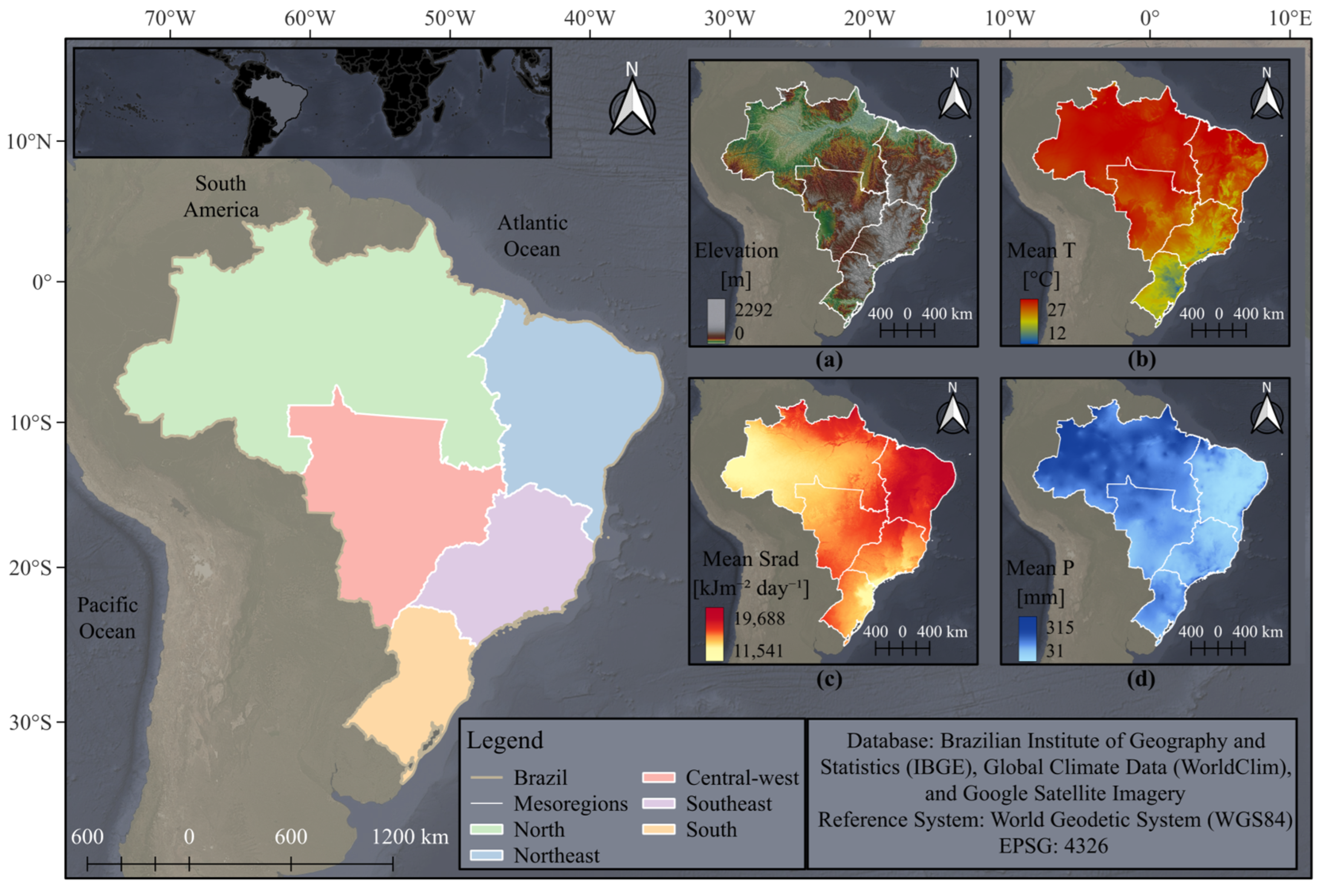
1. Introduction
2. Satellite-Based Mapping Products for Land Use and Land Cover and Agriculture Purposes
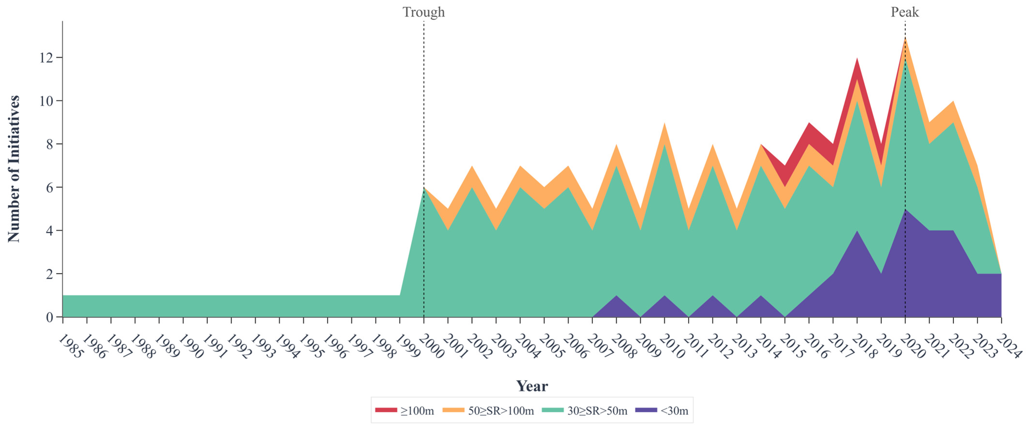
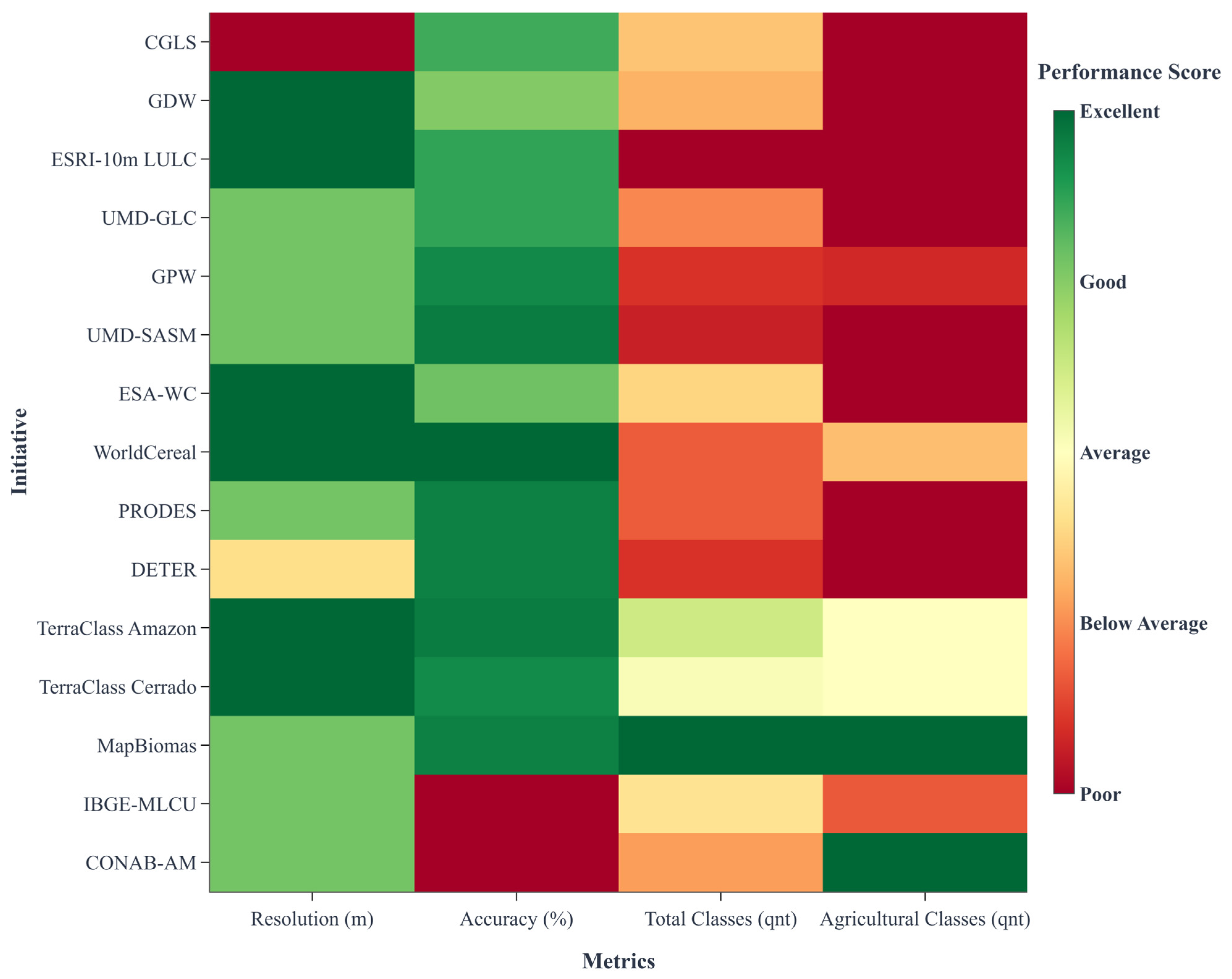
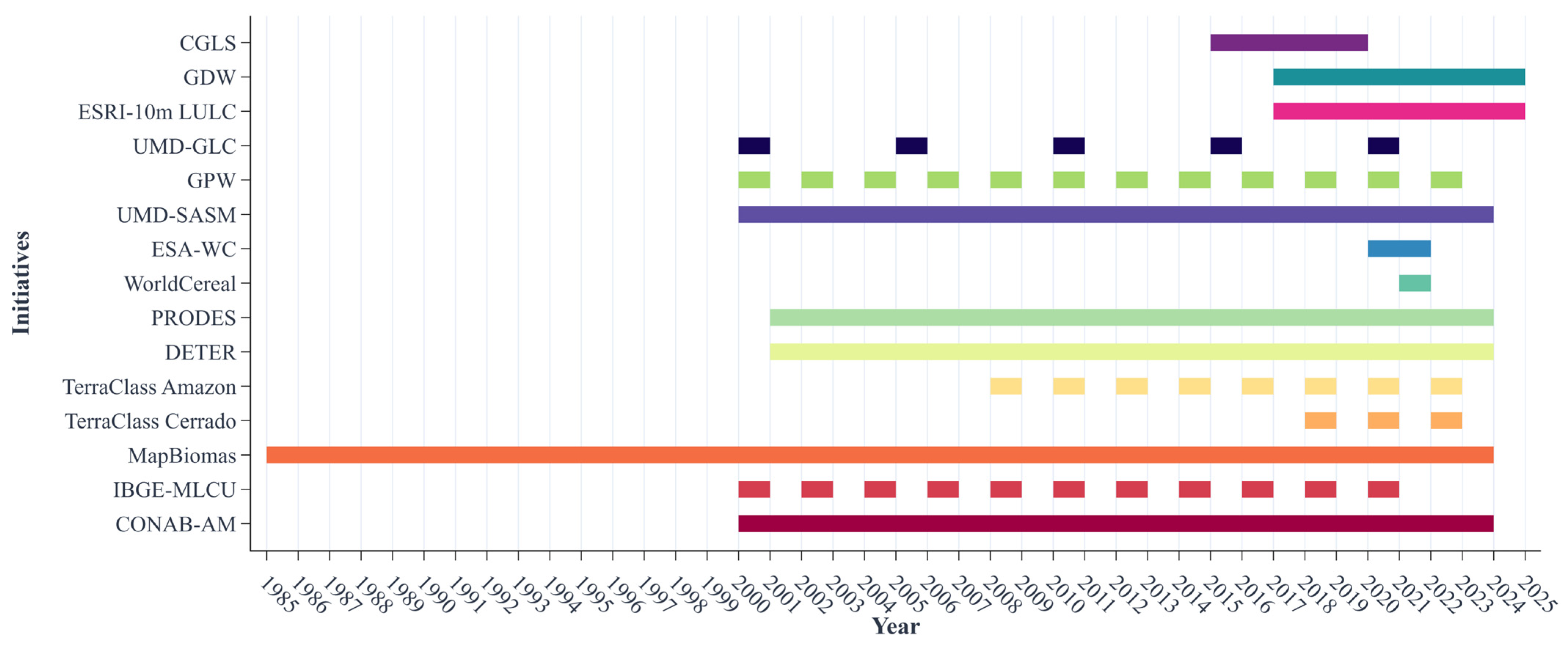
2.1. Overview of Map Products Initiatives
2.2. Map Products at Global and Continental Levels
2.2.1. Copernicus Global Land Cover Service (CGLS) Dynamic Land Cover
2.2.2. Google Dynamic World (GDW)
2.2.3. ESRI Maps for Good Initiative 10 m Annual LULC (ESRI-10m LULC)
2.2.4. The University of Maryland Global Land Cover (UMD-GLC)
2.2.5. Global Pasture Watch (GPW) Global Grassland Class and Extent Maps (GPW)
2.2.6. The University of Maryland South America Soybean Maps (UMD-SASM)
2.2.7. European Space Agency World Cover (ESA-WC)
2.2.8. European Space Agency WorldCereal Crop and Irrigation Mapping (ESA-WorldCereal)
2.3. Map Products at Brazilian National and Regional Levels
2.3.1. National Institute for Spatial Research Deforestation, Warnings, and Vegetation for Brazilian Biomes (PRODES, DETER)
2.3.2. Brazilian Agricultural Research Corporation (EMBRAPA) LULC in the Amazon and Cerrado Biomes (TerraClass)
2.3.3. MapBiomas Project Initiative Collection
2.3.4. Brazilian Institute of Geography and Statistics (IBGE) Monitoring Land Coverage and Use in Brazil (IBGE-MLCU)
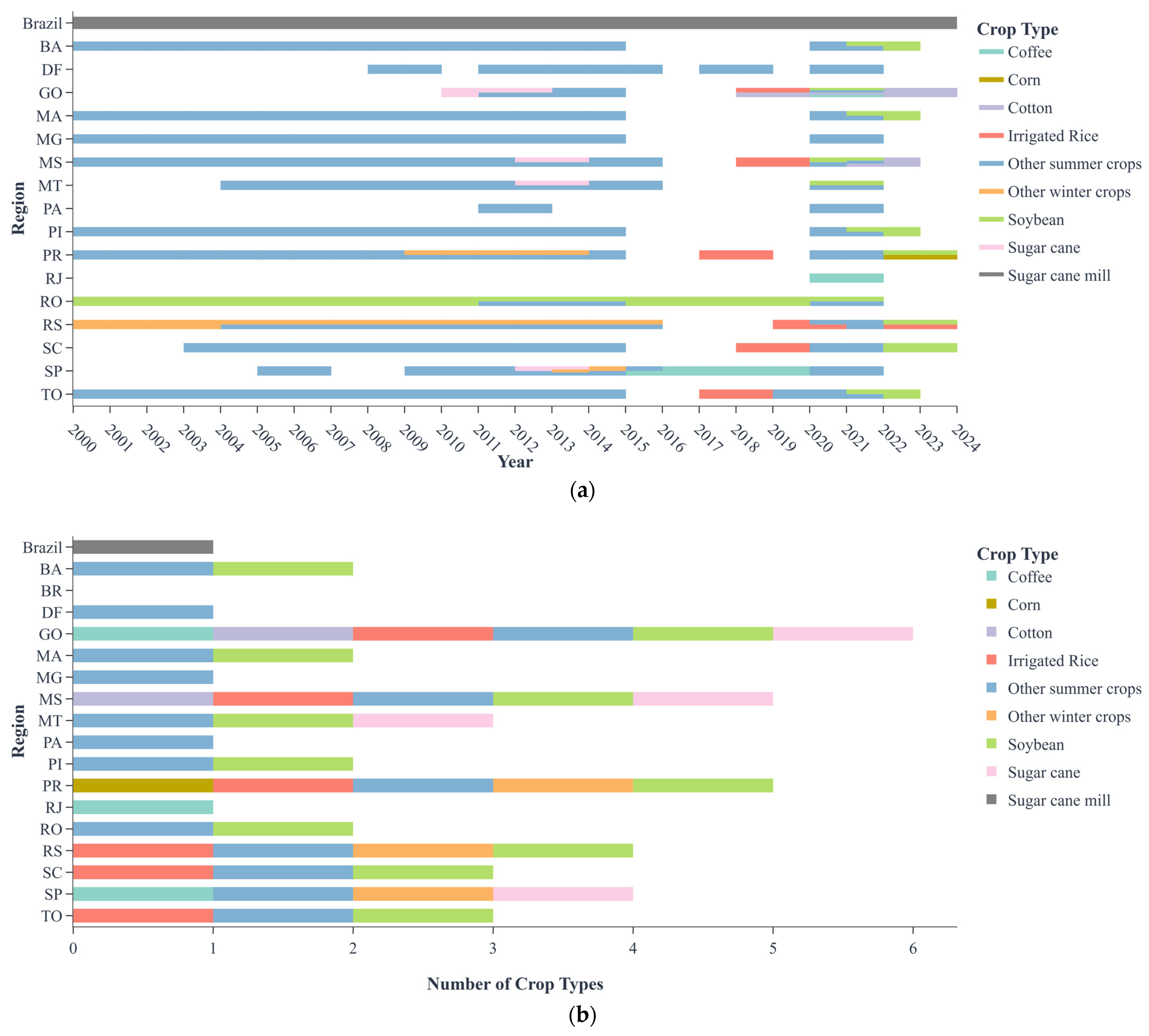
2.3.5. CONAB Agricultural Mapping (CONAB-AM)
3. Discussion
3.1. Data Standardization and Harmonization
3.2. Standardization and Harmonization of Classes and Legends
3.3. Methodology and Product Quality Information
3.4. Other Challenges and Limitations
3.5. Recommendations and Future Directions
4. Conclusions
Author Contributions
Funding
Institutional Review Board Statement
Informed Consent Statement
Data Availability Statement
Acknowledgments
Conflicts of Interest
References
- European Commission. Directive 2007/2/EC of the European Parliament and of the Council of 14 March 2007 Establishing an Infrastructure for Spatial Information in the European Community (INSPIRE) 2007; European Commission: Brussels, Belgium, 2007. [Google Scholar]
- Di Gregorio, A.; Jansen, L.J.M. Land Cover Classification System: Classification Concepts and User Manual; Software Version 2; Food and Agriculture Organization of the United Nations (FAO), Ed.; Environment and natural resources service series GEO-spatial data and information; Food and Agriculture Organization of the United Nations: Rome, Italy, 2005; ISBN 978-92-5-105327-0. [Google Scholar]
- García-Álvarez, D.; Nanu, S.F. Land Use Cover Datasets: A Review. In Land Use Cover Datasets and Validation Tools; García-Álvarez, D., Camacho Olmedo, M.T., Paegelow, M., Mas, J.F., Eds.; Springer International Publishing: Cham, Switzerland, 2022; pp. 47–66. ISBN 978-3-030-90997-0. [Google Scholar]
- Loveland, T.R.; Dwyer, J.L. Landsat: Building a Strong Future. Remote Sens. Environ. 2012, 122, 22–29. [Google Scholar] [CrossRef]
- Potapov, P.; Hansen, M.C.; Pickens, A.; Hernandez-Serna, A.; Tyukavina, A.; Turubanova, S.; Zalles, V.; Li, X.; Khan, A.; Stolle, F.; et al. The Global 2000–2020 Land Cover and Land Use Change Dataset Derived from the Landsat Archive: First Results. Front. Remote Sens. 2022, 3, 856903. [Google Scholar] [CrossRef]
- Verburg, P.H.; Neumann, K.; Nol, L. Challenges in Using Land Use and Land Cover Data for Global Change Studies. Glob. Change Biol. 2011, 17, 974–989. [Google Scholar] [CrossRef]
- Macarringue, L.S.; Bolfe, É.L.; Pereira, P.R.M. Developments in Land Use and Land Cover Classification Techniques in Remote Sensing: A Review. JGIS J. Geogr. Inf. Syst. 2022, 14, 1–28. [Google Scholar] [CrossRef]
- Don, A.; Schumacher, J.; Freibauer, A. Impact of Tropical Land-Use Change on Soil Organic Carbon Stocks—A Meta-Analysis: Soil Organic Carbon and Land-Use Change. Glob. Change Biol. 2011, 17, 1658–1670. [Google Scholar] [CrossRef]
- Foley, J.A.; DeFries, R.; Asner, G.P.; Barford, C.; Bonan, G.; Carpenter, S.R.; Chapin, F.S.; Coe, M.T.; Daily, G.C.; Gibbs, H.K.; et al. Global Consequences of Land Use. Science 2005, 309, 570–574. [Google Scholar] [CrossRef]
- Grimm, N.B.; Faeth, S.H.; Golubiewski, N.E.; Redman, C.L.; Wu, J.; Bai, X.; Briggs, J.M. Global Change and the Ecology of Cities. Science 2008, 319, 756–760. [Google Scholar] [CrossRef]
- Pan, Y.; Birdsey, R.A.; Fang, J.; Houghton, R.; Kauppi, P.E.; Kurz, W.A.; Phillips, O.L.; Shvidenko, A.; Lewis, S.L.; Canadell, J.G.; et al. A Large and Persistent Carbon Sink in the World’s Forests. Science 2011, 333, 988–993. [Google Scholar] [CrossRef]
- Song, X.-P.; Huang, C.; Saatchi, S.S.; Hansen, M.C.; Townshend, J.R. Annual Carbon Emissions from Deforestation in the Amazon Basin between 2000 and 2010. PLoS ONE 2015, 10, e0126754. [Google Scholar] [CrossRef]
- Potapov, P.; Turubanova, S.; Hansen, M.C.; Tyukavina, A.; Zalles, V.; Khan, A.; Song, X.-P.; Pickens, A.; Shen, Q.; Cortez, J. Global Maps of Cropland Extent and Change Show Accelerated Cropland Expansion in the Twenty-First Century. Nat. Food 2021, 3, 19–28. [Google Scholar] [CrossRef]
- Vancutsem, C.; Achard, F.; Pekel, J.-F.; Vieilledent, G.; Carboni, S.; Simonetti, D.; Gallego, J.; Aragão, L.E.O.C.; Nasi, R. Long-Term (1990–2019) Monitoring of Forest Cover Changes in the Humid Tropics. Sci. Adv. 2021, 7, eabe1603. [Google Scholar] [CrossRef]
- Curtis, P.G.; Slay, C.M.; Harris, N.L.; Tyukavina, A.; Hansen, M.C. Classifying Drivers of Global Forest Loss. Science 2018, 361, 1108–1111. [Google Scholar] [CrossRef] [PubMed]
- Estoque, R. A Review of the Sustainability Concept and the State of SDG Monitoring Using Remote Sensing. Remote Sens. 2020, 12, 1770. [Google Scholar] [CrossRef]
- Burke, M.; Driscoll, A.; Lobell, D.B.; Ermon, S. Using Satellite Imagery to Understand and Promote Sustainable Development. Science 2021, 371, eabe8628. [Google Scholar] [CrossRef]
- Karra, K.; Kontgis, C.; Statman-Weil, Z.; Mazzariello, J.C.; Mathis, M.; Brumby, S.P. Global Land Use/Land Cover with Sentinel 2 and Deep Learning. In Proceedings of the 2021 IEEE International Geoscience and Remote Sensing Symposium IGARSS, Brussels, Belgium, 11 July 2021; pp. 4704–4707. [Google Scholar]
- Xu, P.; Tsendbazar, N.-E.; Herold, M.; De Bruin, S.; Koopmans, M.; Birch, T.; Carter, S.; Fritz, S.; Lesiv, M.; Mazur, E.; et al. Comparative Validation of Recent 10 M-Resolution Global Land Cover Maps. Remote Sens. Environ. 2024, 311, 114316. [Google Scholar] [CrossRef]
- Brown, C.F.; Brumby, S.P.; Guzder-Williams, B.; Birch, T.; Hyde, S.B.; Mazzariello, J.; Czerwinski, W.; Pasquarella, V.J.; Haertel, R.; Ilyushchenko, S.; et al. Dynamic World, Near Real-Time Global 10 m Land Use Land Cover Mapping. Sci. Data 2022, 9, 251. [Google Scholar] [CrossRef]
- Buchhorn, M.; Bertels, L.; Smets, B.; De Roo, B.; Lesiv, M.; Tsendbazar, N.-E.; Masiliunas, D.; Li, L. Copernicus Global Land Service: Land Cover 100 m: Version 3 Globe 2015–2019: Algorithm Theoretical Basis Document; Zenodo: Geneva, Switzerland, 2020. [Google Scholar]
- Gomes, V.; Queiroz, G.; Ferreira, K. An Overview of Platforms for Big Earth Observation Data Management and Analysis. Remote Sens. 2020, 12, 1253. [Google Scholar] [CrossRef]
- Velastegui-Montoya, A.; Montalván-Burbano, N.; Carrión-Mero, P.; Rivera-Torres, H.; Sadeck, L.; Adami, M. Google Earth Engine: A Global Analysis and Future Trends. Remote Sens. 2023, 15, 3675. [Google Scholar] [CrossRef]
- Wang, L.; Ma, Y.; Yan, J.; Chang, V.; Zomaya, A.Y. pipsCloud: High Performance Cloud Computing for Remote Sensing Big Data Management and Processing. Future Gener. Comput. Syst. 2018, 78, 353–368. [Google Scholar] [CrossRef]
- Soille, P.; Burger, A.; De Marchi, D.; Kempeneers, P.; Rodriguez, D.; Syrris, V.; Vasilev, V. A Versatile Data-Intensive Computing Platform for Information Retrieval from Big Geospatial Data. Future Gener. Comput. Syst. 2018, 81, 30–40. [Google Scholar] [CrossRef]
- Pebesma, E.; Wagner, W.; Schramm, M.; Von Beringe, A.; Paulik, C.; Neteler, M.; Reiche, J.; Verbesselt, J.; Dries, J.; Goor, E.; et al. OpenEO—A Common, Open Source Interface Between Earth Observation Data Infrastructures and Front-End Applications; Zenodo: Geneva, Switzerland, 2017. [Google Scholar] [CrossRef]
- Atzberger, C. Advances in Remote Sensing of Agriculture: Context Description, Existing Operational Monitoring Systems and Major Information Needs. Remote Sens. 2013, 5, 949–981. [Google Scholar] [CrossRef]
- Whitcraft, A.K.; Vermote, E.F.; Becker-Reshef, I.; Justice, C.O. Cloud Cover throughout the Agricultural Growing Season: Impacts on Passive Optical Earth Observations. Remote Sens. Environ. 2015, 156, 438–447. [Google Scholar] [CrossRef]
- Whitcraft, A.K.; Becker-Reshef, I.; Justice, C.O. Agricultural Growing Season Calendars Derived from MODIS Surface Reflectance. Int. J. Digit. Earth 2015, 8, 173–197. [Google Scholar] [CrossRef]
- Whitcraft, A.; Becker-Reshef, I.; Justice, C. A Framework for Defining Spatially Explicit Earth Observation Requirements for a Global Agricultural Monitoring Initiative (GEOGLAM). Remote Sens. 2015, 7, 1461–1481. [Google Scholar] [CrossRef]
- Song, X.-P.; Potapov, P.V.; Krylov, A.; King, L.; Di Bella, C.M.; Hudson, A.; Khan, A.; Adusei, B.; Stehman, S.V.; Hansen, M.C. National-Scale Soybean Mapping and Area Estimation in the United States Using Medium Resolution Satellite Imagery and Field Survey. Remote Sens. Environ. 2017, 190, 383–395. [Google Scholar] [CrossRef]
- Wulder, M.A.; Masek, J.G.; Cohen, W.B.; Loveland, T.R.; Woodcock, C.E. Opening the Archive: How Free Data Has Enabled the Science and Monitoring Promise of Landsat. Remote Sens. Environ. 2012, 122, 2–10. [Google Scholar] [CrossRef]
- Whitcraft, A.; Becker-Reshef, I.; Killough, B.; Justice, C. Meeting Earth Observation Requirements for Global Agricultural Monitoring: An Evaluation of the Revisit Capabilities of Current and Planned Moderate Resolution Optical Earth Observing Missions. Remote Sens. 2015, 7, 1482–1503. [Google Scholar] [CrossRef]
- You, L.; Sun, Z. Mapping Global Cropping System: Challenges, Opportunities, and Future Perspectives. Crop Environ. 2022, 1, 68–73. [Google Scholar] [CrossRef]
- Sishodia, R.P.; Ray, R.L.; Singh, S.K. Applications of Remote Sensing in Precision Agriculture: A Review. Remote Sens. 2020, 12, 3136. [Google Scholar] [CrossRef]
- Khanal, S.; Kc, K.; Fulton, J.P.; Shearer, S.; Ozkan, E. Remote Sensing in Agriculture—Accomplishments, Limitations, and Opportunities. Remote Sens. 2020, 12, 3783. [Google Scholar] [CrossRef]
- Fuentes-Peñailillo, F.; Gutter, K.; Vega, R.; Silva, G.C. Transformative Technologies in Digital Agriculture: Leveraging Internet of Things, Remote Sensing, and Artificial Intelligence for Smart Crop Management. JSAN J. Sens. Actuator Netw. 2024, 13, 39. [Google Scholar] [CrossRef]
- Whitcraft, A.K.; McNairn, H.; Lemoine, G.; LeToan, T.; Sobue, S.-I. The Power of Synthetic Aperture Radar for Global Agricultural Monitoring. In Proceedings of the Global Agricultural Monitoring (GEOGLAM); CEOS: Geneva, Switzerland, 2016; pp. 1–4. [Google Scholar]
- Muruganantham, P.; Wibowo, S.; Grandhi, S.; Samrat, N.H.; Islam, N. A Systematic Literature Review on Crop Yield Prediction with Deep Learning and Remote Sensing. Remote Sens. 2022, 14, 1990. [Google Scholar] [CrossRef]
- Ji, Z.; Pan, Y.; Zhu, X.; Wang, J.; Li, Q. Prediction of Crop Yield Using Phenological Information Extracted from Remote Sensing Vegetation Index. Sensors 2021, 21, 1406. [Google Scholar] [CrossRef] [PubMed]
- Getahun, S.; Kefale, H.; Gelaye, Y. Application of Precision Agriculture Technologies for Sustainable Crop Production and Environmental Sustainability: A Systematic Review. Sci. World J. 2024, 2024, 2126734. [Google Scholar] [CrossRef] [PubMed]
- Aznar-Sánchez, J.A.; Piquer-Rodríguez, M.; Velasco-Muñoz, J.F.; Manzano-Agugliaro, F. Worldwide Research Trends on Sustainable Land Use in Agriculture. Land Use Policy 2019, 87, 104069. [Google Scholar] [CrossRef]
- Prudente, V.H.R.; Skakun, S.; Oldoni, L.V.; Xaud, H.A.M.; Xaud, M.R.; Adami, M.; Sanches, I.D. Multisensor Approach to Land Use and Land Cover Mapping in Brazilian Amazon. ISPRS J. Photogramm. Remote Sens. 2022, 189, 95–109. [Google Scholar] [CrossRef]
- Adami, M.; Moreira, M.A.; Rudorff, B.F.T.; Freitas, C.D.C.; Faria, R.T.D. Expansão Direta Na Estimativa de Culturas Agrícolas Por Meio de Segmentos Regulares. Rev. Bras. Cartogr. 2009, 57, 22–27. [Google Scholar] [CrossRef]
- Benami, E.; Jin, Z.; Carter, M.R.; Ghosh, A.; Hijmans, R.J.; Hobbs, A.; Kenduiywo, B.; Lobell, D.B. Uniting Remote Sensing, Crop Modelling and Economics for Agricultural Risk Management. Nat. Rev. Earth Environ. 2021, 2, 140–159. [Google Scholar] [CrossRef]
- Mahlayeye, M.; Darvishzadeh, R.; Nelson, A. Cropping Patterns of Annual Crops: A Remote Sensing Review. Remote Sens. 2022, 14, 2404. [Google Scholar] [CrossRef]
- Jain, M.; Mondal, P.; DeFries, R.S.; Small, C.; Galford, G.L. Mapping Cropping Intensity of Smallholder Farms: A Comparison of Methods Using Multiple Sensors. Remote Sens. Environ. 2013, 134, 210–223. [Google Scholar] [CrossRef]
- Vishnoi, S.; Goel, R.K. Climate Smart Agriculture for Sustainable Productivity and Healthy Landscapes. Environ. Sci. Policy 2024, 151, 103600. [Google Scholar] [CrossRef]
- FAO—Food and Agriculture Organization of the United Nations. FAOSTAT: Top 20 Commodities, Export Value by Country 2022. Available online: https://www.fao.org/faostat/en/#rankings/major_commodities_exports (accessed on 11 November 2024).
- IBGE—Brazilian Institute of Geography and Statistics. Produção Agrícola Municipal 2023; IBGE: Rio de Janeiro, Brazil, 2024. [Google Scholar]
- Cherubin, M.R.; Damian, J.M.; Tavares, T.R.; Trevisan, R.G.; Colaço, A.F.; Eitelwein, M.T.; Martello, M.; Inamasu, R.Y.; Pias, O.H.D.C.; Molin, J.P. Precision Agriculture in Brazil: The Trajectory of 25 Years of Scientific Research. Agriculture 2022, 12, 1882. [Google Scholar] [CrossRef]
- IBGE—Brazilian Institute of Geography and Statistics. IBGE Cidades: Panorama Brasil. Available online: https://cidades.ibge.gov.br/brasil/panorama (accessed on 19 September 2024).
- Tozer, B.; Sandwell, D.T.; Smith, W.H.F.; Olson, C.; Beale, J.R.; Wessel, P. Global Bathymetry and Topography at 15 Arc Sec: SRTM15+. Earth Space Sci. 2019, 6, 1847–1864. [Google Scholar] [CrossRef]
- Fick, S.E.; Hijmans, R.J. WorldClim 2: New 1-km Spatial Resolution Climate Surfaces for Global Land Areas. Int. J. Climatol. 2017, 37, 4302–4315. [Google Scholar] [CrossRef]
- Aparecido, L.E.D.O.; Batista, R.M.; Moraes, J.R.D.S.C.D.; Costa, C.T.S.; Moraes-Oliveira, A.F.D. Agricultural Zoning of Climate Risk for Physalis Peruviana Cultivation in Southeastern Brazil. Pesqui. Agropecuária Bras. 2019, 54, e00057. [Google Scholar] [CrossRef]
- Silva, M.A.S.D.; Matos, L.N.; Santos, F.E.D.O.; Dompieri, M.H.G.; Moura, F.R.D. Tracking the Connection Between Brazilian Agricultural Diversity and Native Vegetation Change by a Machine Learning Approach. IEEE Lat. Am. Trans. 2022, 20, 2371–2380. [Google Scholar] [CrossRef]
- Cerri, C.E.P.; Sparovek, G.; Bernoux, M.; Easterling, W.E.; Melillo, J.M.; Cerri, C.C. Tropical Agriculture and Global Warming: Impacts and Mitigation Options. Sci. Agric. 2007, 64, 83–99. [Google Scholar] [CrossRef]
- Harvey, C.A.; Chacón, M.; Donatti, C.I.; Garen, E.; Hannah, L.; Andrade, A.; Bede, L.; Brown, D.; Calle, A.; Chará, J.; et al. Climate-Smart Landscapes: Opportunities and Challenges for Integrating Adaptation and Mitigation in Tropical Agriculture. Conserv. Lett. 2014, 7, 77–90. [Google Scholar] [CrossRef]
- CONAB—Brazilian National Supply Company. Calendário de Plantio e Colheita de grãos no Brasil 2022; CONAB: Brasília, Brazil, 2022. [Google Scholar]
- Adami, M.; Campos, P.M.; Fernandes, L.B.; Souza, R.d.S.; Lima, F.A.S.; dos Santos, P.A.; de Santana, C.T.C.; Santos, C.M.R.; Sanches, I.D. Rumo a Estimativa Objetivas de Safras Agrícolas; Instituto Nacional de Pesquisas Espaciais (INPE): São Paulo, Brazil, 2023; p. e156102. [Google Scholar]
- Campos, P.M.; Souza, R.; Lima, F.A.; Fernandes, L.B.; Adami, M.; Gotijo, E.; Piffer, T.; de Santana, C.T.C.; Santos, C.; Sanches, I.D. Estimativa E Mapeamento de áReas Cultivadas Com Soja. In Proceedings of the Anais do XX Simpósio Brasileiro de Sensoriamento Remoto; Gherardi, D.F.M., Sanches, I.D.A., de Aragão, L.E.O.e.C., Eds.; INPF: Florianópolis, Brasil, 2023; Volume 20, pp. 709–711. [Google Scholar]
- INPE—National Institute for Space Research. INPE Apresenta Dados Inéditos de Desmatamento para Todo Brasil; INPE: São Paulo, Brazil, 2022. [Google Scholar]
- FAO—Food and Agriculture Organization of the United Nations. FAOSTAT Land Use Statistics. Available online: https://www.fao.org/faostat/en/#data/RL (accessed on 20 March 2025).
- Alencar, A.; Shimbo, J.Z.; Lenti, F.; Balzani Marques, C.; Zimbres, B.; Rosa, M.; Arruda, V.; Castro, I.; Fernandes Márcico Ribeiro, J.; Varela, V.; et al. Mapping Three Decades of Changes in the Brazilian Savanna Native Vegetation Using Landsat Data Processed in the Google Earth Engine Platform. Remote Sens. 2020, 12, 924. [Google Scholar] [CrossRef]
- Meyfroidt, P.; Roy Chowdhury, R.; De Bremond, A.; Ellis, E.C.; Erb, K.-H.; Filatova, T.; Garrett, R.D.; Grove, J.M.; Heinimann, A.; Kuemmerle, T.; et al. Middle-Range Theories of Land System Change. Glob. Environ. Change 2018, 53, 52–67. [Google Scholar] [CrossRef]
- García-Álvarez, D.; Camacho Olmedo, M.T.; Mas, J.-F.; Paegelow, M. Land Use Cover Mapping, Modelling and Validation. A Background. In Land Use Cover Datasets and Validation Tools; García-Álvarez, D., Camacho Olmedo, M.T., Paegelow, M., Mas, J.F., Eds.; Springer International Publishing: Cham, Switzerland, 2022; pp. 21–33. ISBN 978-3-030-90997-0. [Google Scholar]
- Hansen, M.C.; Defries, R.S.; Townshend, J.R.G.; Sohlberg, R. Global Land Cover Classification at 1 Km Spatial Resolution Using a Classification Tree Approach. Int. J. Remote Sens. 2000, 21, 1331–1364. [Google Scholar] [CrossRef]
- Loveland, T.R.; Reed, B.C.; Brown, J.F.; Ohlen, D.O.; Zhu, Z.; Yang, L.; Merchant, J.W. Development of a Global Land Cover Characteristics Database and IGBP DISCover from 1 Km AVHRR Data. Int. J. Remote Sens. 2000, 21, 1303–1330. [Google Scholar] [CrossRef]
- Bartholomé, E.; Belward, A.S. GLC2000: A New Approach to Global Land Cover Mapping from Earth Observation Data. Int. J. Remote Sens. 2005, 26, 1959–1977. [Google Scholar] [CrossRef]
- Fritz, S.; Bartholomé, E.; Belward, A.; Hartley, A.; Hans-Jurgen, S.; Eva, H.; Mayaux, P.; Bartalev, S.; Latifovic, R.; Kolmert, S.; et al. Harmonisation, Mosaicing and Production of the Global Land Cover 2000 Database (Beta Version); Commission, E., Centre, J.R., Eds.; European Union Publications Office: Brussels, Belgium, 2003; ISBN 92-894-6332-5. [Google Scholar]
- Hua, T.; Zhao, W.; Liu, Y.; Wang, S.; Yang, S. Spatial Consistency Assessments for Global Land-Cover Datasets: A Comparison among GLC2000, CCI LC, MCD12, GLOBCOVER and GLCNMO. Remote Sens. 2018, 10, 1846. [Google Scholar] [CrossRef]
- Biancalani, R.; Nachtergaele, F.; Petri, M.; Bunning, S. Land Degradation Assessment in Drylands. LADA Project Methodology and Results; LADA Project; FAO: Rome, Italy, 2013; pp. 1–63. [Google Scholar]
- Latham, J.; Cumani, R.; Rosati, I.; Bloise, M. Global Land Cover SHARE (GLC-SHARE) Database Beta-Realease Version 1.0—2014; GLC-SHARE; FAO: Rome, Italy, 2014; pp. 1–40. [Google Scholar]
- Tang, F.H.M.; Nguyen, T.H.; Conchedda, G.; Casse, L.; Tubiello, F.N.; Maggi, F. CROPGRIDS: A Global Geo-Referenced Dataset of 173 Crops. Sci. Data 2024, 11, 413. [Google Scholar] [CrossRef] [PubMed]
- See, L.; Schepaschenko, D.; Lesiv, M.; McCallum, I.; Fritz, S.; Comber, A.; Perger, C.; Schill, C.; Zhao, Y.; Maus, V.; et al. Building a Hybrid Land Cover Map with Crowdsourcing and Geographically Weighted Regression. ISPRS J. Photogramm. Remote Sens. 2015, 103, 48–56. [Google Scholar] [CrossRef]
- Liu, H.; Gong, P.; Wang, J.; Clinton, N.; Bai, Y.; Liang, S. Annual Dynamics of Global Land Cover and Its Long-Term Changes from 1982 to 2015. Earth Syst. Sci. Data 2020, 12, 1217–1243. [Google Scholar] [CrossRef]
- ESA—European Space Agency. Land Cover CCI Product User Guide Version 2; ESA CCI Land Cover time-series v2.0.7 (1992–2015); European Space Agency, European Union: Brussels, Belgium, 2017; pp. 1–105. [Google Scholar]
- Chen, J.; Chen, J.; Liao, A.; Cao, X.; Chen, L.; Chen, X.; He, C.; Han, G.; Peng, S.; Lu, M.; et al. Global Land Cover Mapping at 30m Resolution: A POK-Based Operational Approach. ISPRS J. Photogramm. Remote Sens. 2015, 103, 7–27. [Google Scholar] [CrossRef]
- Ping, T.; Hongwei, Z.; Yongchao, Z.; Zhenguo, N.; Bo, Z.; Changmiao, H.; Xiaojun, S.; Institute of Remote Sensing and Digital Earth, Chinese Academy of Sciences; National Geomatics Center of China; Institute of Electronics, Chinese Academy of Sciences. Practice and Thoughts of the Automatic Processing of Multispectral Images with 30 m Spatial Resolution on the Global Scale. Natl. Remote Sens. Bull. 2014, 18, 231–253. [Google Scholar] [CrossRef]
- Wang, J.; Zhao, Y.; Li, C.; Yu, L.; Liu, D.; Gong, P. Mapping Global Land Cover in 2001 and 2010 with Spatial-Temporal Consistency at 250m Resolution. ISPRS J. Photogramm. Remote Sens. 2015, 103, 38–47. [Google Scholar] [CrossRef]
- Xie, H.; Tong, X.; Meng, W.; Liang, D.; Wang, Z.; Shi, W. A Multilevel Stratified Spatial Sampling Approach for the Quality Assessment of Remote-Sensing-Derived Products. IEEE J. Sel. Top. Appl. Earth Obs. Remote Sens. 2015, 8, 4699–4713. [Google Scholar] [CrossRef]
- Friedl, M.A.; Sulla-Menashe, D.; Tan, B.; Schneider, A.; Ramankutty, N.; Sibley, A.; Huang, X. MODIS Collection 5 Global Land Cover: Algorithm Refinements and Characterization of New Datasets. Remote Sens. Environ. 2010, 114, 168–182. [Google Scholar] [CrossRef]
- Friedl, M.A.; McIver, D.K.; Hodges, J.C.F.; Zhang, X.Y.; Muchoney, D.; Strahler, A.H.; Woodcock, C.E.; Gopal, S.; Schneider, A.; Cooper, A.; et al. Global Land Cover Mapping from MODIS: Algorithms and Early Results. Remote Sens. Environ. 2002, 83, 287–302. [Google Scholar] [CrossRef]
- Sulla-Menashe, D.; Gray, J.M.; Abercrombie, S.P.; Friedl, M.A. Hierarchical Mapping of Annual Global Land Cover 2001 to Present: The MODIS Collection 6 Land Cover Product. Remote Sens. Environ. 2019, 222, 183–194. [Google Scholar] [CrossRef]
- Kobayashi, T.; Tateishi, R.; Alsaaideh, B.; Sharma, R.C.; Wakaizumi, T.; Miyamoto, D.; Bai, X.; Long, B.D.; Gegentana, G.; Maitiniyazi, A.; et al. Production of Global Land Cover Data—GLCNMO2013. JGG J. Geogr. Geol. 2017, 9, 1. [Google Scholar] [CrossRef]
- Tateishi, R.; Uriyangqai, B.; Al-Bilbisi, H.; Ghar, M.A.; Tsend-Ayush, J.; Kobayashi, T.; Kasimu, A.; Hoan, N.T.; Shalaby, A.; Alsaaideh, B.; et al. Production of Global Land Cover Data—GLCNMO. Int. J. Digit. Earth 2011, 4, 22–49. [Google Scholar] [CrossRef]
- Bicheron, P.; Defourny, P.; Brockmann, C.; Schouten, L.; Vancutsem, C.; Huc, M.; Bontemps, S.; Leroy, M.; Achard, F.; Herold, M.; et al. GLOBCOVER Products Description and Validation Report; European Space Agency, UCLouvain: Louvain-la-Neuve, Belgium, 2008; pp. 1–47. [Google Scholar]
- Gong, P.; Wang, J.; Yu, L.; Zhao, Y.; Zhao, Y.; Liang, L.; Niu, Z.; Huang, X.; Fu, H.; Liu, S.; et al. Finer Resolution Observation and Monitoring of Global Land Cover: First Mapping Results with Landsat TM and ETM+ Data. Int. J. Remote Sens. 2013, 34, 2607–2654. [Google Scholar] [CrossRef]
- Yu, L.; Wang, J.; Gong, P. Improving 30 m Global Land-Cover Map FROM-GLC with Time Series MODIS and Auxiliary Data Sets: A Segmentation-Based Approach. Int. J. Remote Sens. 2013, 34, 5851–5867. [Google Scholar] [CrossRef]
- Tsendbazar, N.-E.; Tarko, A.; Li, L.; Herold, M.; Lesiv, M.; Fritz, S.; Maus, V. Copernicus Global Land Service: Land Cover 100 m: Version 3 Globe 2015–2019: Validation Report; Zenodo: Geneva, Switzerland, 2021. [Google Scholar]
- Zanaga, D.; Van De Kerchove, R.; Daems, D.; De Keersmaecker, W.; Brockmann, C.; Kirches, G.; Wevers, J.; Cartus, O.; Santoro, M.; Fritz, S.; et al. ESA WorldCover 10 m 2021 V200; Zenodo: Geneva, Switzerland, 2022. [Google Scholar]
- Zanaga, D.; Van De Kerchove, R.; De Keersmaecker, W.; Souverijns, N.; Brockmann, C.; Quast, R.; Wevers, J.; Grosu, A.; Paccini, A.; Vergnaud, S.; et al. ESA WorldCover 10 m 2020 V100; Zenodo: Geneva, Switzerland, 2021. [Google Scholar]
- Schultz, M.; Voss, J.; Auer, M.; Carter, S.; Zipf, A. Open Land Cover from OpenStreetMap and Remote Sensing. Int. J. Appl. Earth Obs. Geoinf. 2017, 63, 206–213. [Google Scholar] [CrossRef]
- Defries, R.S.; Townshend, J.R.G. NDVI-Derived Land Cover Classifications at a Global Scale. Int. J. Remote Sens. 1994, 15, 3567–3586. [Google Scholar] [CrossRef]
- Song, X.-P.; Hansen, M.C.; Potapov, P.; Adusei, B.; Pickering, J.; Adami, M.; Lima, A.; Zalles, V.; Stehman, S.V.; Di Bella, C.M.; et al. Massive Soybean Expansion in South America since 2000 and Implications for Conservation. Nat. Sustain. 2021, 4, 784–792. [Google Scholar] [CrossRef]
- UMD—University of Maryland; GLAD—Global Land Analysis and Discovery Laboratory; Hansen, M.C.; Potapov, P. Global Land Analysis & Discovery (GLAD): Commodity Crop Mapping and Monitoring in South America. Available online: https://glad.umd.edu/projects/commodity-crop-mapping-and-monitoring-south-america (accessed on 11 September 2024).
- Venter, Z.S.; Barton, D.N.; Chakraborty, T.; Simensen, T.; Singh, G. Global 10 m Land Use Land Cover Datasets: A Comparison of Dynamic World, World Cover and Esri Land Cover. Remote Sens. 2022, 14, 4101. [Google Scholar] [CrossRef]
- Fritz, S.; See, L.; McCallum, I.; You, L.; Bun, A.; Moltchanova, E.; Duerauer, M.; Albrecht, F.; Schill, C.; Perger, C.; et al. Mapping Global Cropland and Field Size. Glob. Change Biol. 2015, 21, 1980–1992. [Google Scholar] [CrossRef]
- Fritz, S.; You, L.; Bun, A.; See, L.; McCallum, I.; Schill, C.; Perger, C.; Liu, J.; Hansen, M.; Obersteiner, M. Cropland for Sub-Saharan Africa: A Synergistic Approach Using Five Land Cover Data Sets: A New Calibrated Cropland Data Set. Geophys. Res. Lett. 2011, 38, L04404. [Google Scholar] [CrossRef]
- Pittman, K.; Hansen, M.C.; Becker-Reshef, I.; Potapov, P.V.; Justice, C.O. Estimating Global Cropland Extent with Multi-Year MODIS Data. Remote Sens. 2010, 2, 1844–1863. [Google Scholar] [CrossRef]
- Teluguntla, P.; Thenkabail, P.S.; Xiong, J.; Gumma, K.M.; Giri, C.; Milesi, C.; Mutlu, O.; Congalton, R.G.; Tilton, J.; Sankey, T.T.; et al. Global Food Security Support Analysis Data at Nominal 1 km (GFSAD1km) Derived from Remote Sensing in Support of Food Security in the Twenty-First Century: Current Achievements and Future Possibilities. In Land Resources Monitoring, Modeling, and Mapping with remote Sensing; Remote Sensing Handbook; CRC Press, Taylor and francis Group: Boca Raton, FL, USA, 2015; Volume 2, p. 30. ISBN 978-0-429-08944-2. [Google Scholar]
- USGS—United States Geological Survey; Earth Resources Observation and Science (EROS) Center. NASA Making Earth System Data Records for Use in Research Environments (MEaSUREs) Global Food Security-Support Analysis Data (GFSAD) 1 km Datasets: User Guide; National Aeronautics and Space Administration (NASA) and the United States Geological Survey (USGS): Sioux Falls, SD, USA, 2017; pp. 1–15. [Google Scholar]
- Rembold, F.; Meroni, M.; Urbano, F.; Csak, G.; Kerdiles, H.; Perez-Hoyos, A.; Lemoine, G.; Leo, O.; Negre, T. ASAP: A New Global Early Warning System to Detect Anomaly Hot Spots of Agricultural Production for Food Security Analysis. Agric. Syst. 2019, 168, 247–257. [Google Scholar] [CrossRef]
- Salmon, J.M.; Friedl, M.A.; Frolking, S.; Wisser, D.; Douglas, E.M. Global Rain-Fed, Irrigated, and Paddy Croplands: A New High Resolution Map Derived from Remote Sensing, Crop Inventories and Climate Data. Int. J. Appl. Earth Obs. Geoinf. 2015, 38, 321–334. [Google Scholar] [CrossRef]
- Lu, M.; Wu, W.; You, L.; See, L.; Fritz, S.; Yu, Q.; Wei, Y.; Chen, D.; Yang, P.; Xue, B. A Cultivated Planet in 2010—Part 1: The Global Synergy Cropland Map. Earth Syst. Sci. Data 2020, 12, 1913–1928. [Google Scholar] [CrossRef]
- Yu, Q.; You, L.; Wood-Sichra, U.; Ru, Y.; Joglekar, A.K.B.; Fritz, S.; Xiong, W.; Lu, M.; Wu, W.; Yang, P. A Cultivated Planet in 2010—Part 2: The Global Gridded Agricultural-Production Maps. Earth Syst. Sci. Data 2020, 12, 3545–3572. [Google Scholar] [CrossRef]
- Waldner, F.; Fritz, S.; Di Gregorio, A.; Plotnikov, D.; Bartalev, S.; Kussul, N.; Gong, P.; Thenkabail, P.; Hazeu, G.; Klein, I.; et al. A Unified Cropland Layer at 250 m for Global Agriculture Monitoring. Data 2016, 1, 3. [Google Scholar] [CrossRef]
- Gumma, M.K.; Thenkabail, P.S.; Teluguntla, P.G.; Oliphant, A.; Xiong, J.; Giri, C.; Pyla, V.; Dixit, S.; Whitbread, A.M. Agricultural Cropland Extent and Areas of South Asia Derived Using Landsat Satellite 30-m Time-Series Big-Data Using Random Forest Machine Learning Algorithms on the Google Earth Engine Cloud. GISci. Remote Sens. 2020, 57, 302–322. [Google Scholar] [CrossRef]
- Phalke, A.R.; Özdoğan, M.; Thenkabail, P.S.; Erickson, T.; Gorelick, N.; Yadav, K.; Congalton, R.G. Mapping Croplands of Europe, Middle East, Russia, and Central Asia Using Landsat, Random Forest, and Google Earth Engine. ISPRS J. Photogramm. Remote Sens. 2020, 167, 104–122. [Google Scholar] [CrossRef]
- Büttner, G. CORINE Land Cover and Land Cover Change Products. In Land Use and Land Cover Mapping in Europe: Practices & Trends; Manakos, I., Braun, M., Eds.; Remote Sensing and Digital Image Processing; Springer: Dordrecht, The Netherlands, 2014; Volume 18, pp. 55–74. ISBN 978-94-007-7969-3. [Google Scholar]
- Buttner, G.; Kosztra, B.; Kleeschulte, S.; Hazeu, G.; Vittek, M.; Schroder, C.; Littkopf, A. Copernicus Land Monitoring Service: Corine Land Cover (from 1990 to 2018) and Corine Land Cover Changes User Manual; Copernicus Land Monitoring Service (CLMS), European Space Agency: Copenhagem, Denmark, 2021; p. 129. [Google Scholar]
- FAO—Food and Agriculture Organization of the United Nations. AFRICOVER: Land Cover Classification.; Food and Agriculture Organization of The United Nations (FAO): Rome, Italy, 1997; p. 84. [Google Scholar]
- Jin, S.; Homer, C.; Yang, L.; Danielson, P.; Dewitz, J.; Li, C.; Zhu, Z.; Xian, G.; Howard, D. Overall Methodology Design for the United States National Land Cover Database 2016 Products. Remote Sens. 2019, 11, 2971. [Google Scholar] [CrossRef]
- Stone, T.A.; Schlesinger, P.; Houghton, R.A.; Woodwell, G.M. A Map of the Vegetation of South America Based on Satellite Imagery. ASPRS Am. Soc. Photogramm. Remote Sens. 1994, 60, 541–551. [Google Scholar]
- EMBRAPA—Brazilian Agricultural Research Corporation; INPE—National Institute for Space Research. TerraClass: Download de Dados. Available online: https://www.terraclass.gov.br/download-de-dados (accessed on 11 September 2024).
- Souza, C.M.; Shimbo, J.Z.; Rosa, M.R.; Parente, L.L.; Alencar, A.A.; Rudorff, B.F.T.; Hasenack, H.; Matsumoto, M.; Ferreira, L.G.; Souza-Filho, P.W.M.; et al. Reconstructing Three Decades of Land Use and Land Cover Changes in Brazilian Biomes with Landsat Archive and Earth Engine. Remote Sens. 2020, 12, 2735. [Google Scholar] [CrossRef]
- MapBiomas.parent Plataforma MapBiomas Brasil. Available online: https://plataforma.brasil.mapbiomas.org/ (accessed on 11 September 2024).
- Buchhorn, M.; Smets, B.; Bertels, L.; De Roo, B.; Lesiv, M.; Tsendbazar, N.-E.; Li, L.; Tarko, A. Copernicus Global Land Service: Land Cover 100 m: Version 3 Globe 2015–2019: Product User Manual; Zenodo: Geneva, Switzerland, 2021. [Google Scholar]
- Jones, A.; Fernandez-Ugalde, O.; Scarpa, S. LUCAS 2015 Topsoil Survey. Presentation of Dataset and Results.; Joint Research Center (JCR) Technical Reports; Publications Office of the European Union: Luxemburg, 2020; p. 83. [Google Scholar]
- Penman, J.; Gytarsky, M.; Hiraishi, T.; Krug, T.; Kruger, D.; Pipatti, R.; Buendia, L.; Miwa, K.; Ngara, T.; Tanabe, K.; et al. Good Practice Guidance for Land Use, Land-Use Change and Forestry. The Intergovernmental Panel on Climate Change; Institute for Global Environmental Strategies (IGES) for the IPCC: Hayama, Japan, 2003; ISBN 978-4-88788-003-0. [Google Scholar]
- Anderson, J.R.; Hardy, E.E.; Roach, J.T.; Witmer, R.E. A Land Use and Land Cover Classification System for Use with Remote Sensor Data; USGS Numbered Series; United States Geological Survey, USGS: Washington, DC, USA, 1976; p. 28. [Google Scholar]
- Brown, C.F.; Brumby, S.P.; Guzder-Williams, B.; Birch, T.; Hyde, S.B.; Mazzariello, J.; Czerwinski, W.; Pasquarella, V.J.; Haertel, R.; Ilyushchenko, S.; et al. Dynamic World Test Tiles; Zenodo: Geneva, Switzerland, 2021. [Google Scholar]
- Impact Observatory [IO] Impact Observatory Maps for Good: Open Acess Global Land Cover Maps. Available online: https://www.impactobservatory.com/maps-for-good/ (accessed on 27 September 2024).
- ESRI—Environmental Systems Research Institute; IO—Impact Observatory. ESRI Sentinel-2 Land Cover Explorer. Available online: https://livingatlas.arcgis.com/landcoverexplorer/ (accessed on 25 September 2024).
- IO—Impact Observatory. Sentinel-Hub EO Browser: IO Land Use Land Cover Map (9-Class). Available online: https://apps.sentinel-hub.com/eo-browser/?zoom=10&lat=41.9&lng=12.5&themeId=DEFAULT-THEME&visualizationUrl=U2FsdGVkX1932REiIrm8sGm%2F%2BnudLl%2FH89TjvzZuhIuxaPKX1fKxVblLDFyYFDYyIPeqHkmoKGeRx5%2BwMHTFmat%2BBt5P1wLW%2Fnz5To3Db8CnIcQKMv%2FhcI2O3j92c75G&datasetId=IO_LULC_10M_ANNUAL&fromTime=2022-01-01T00%3A00%3A00.000Z&toTime=2022-01-01T23%3A59%3A59.999Z&layerId=IO-LAND-USE-LAND-COVER-MAP&demSource3D=%22MAPZEN%22 (accessed on 27 September 2024).
- UMD—University of Maryland; GLAD—Global Land Analysis and Discovery Laboratory. Global Land Cover and Land Use 2000 and 2020. Available online: https://storage.googleapis.com/earthenginepartners-hansen/GLCLU2000-2020/v2/download.html (accessed on 11 September 2024).
- UMD—University of Maryland; GLAD—Global Land Analysis and Discovery Laboratory. Global Land Cover and Land Use Change, 2000–2020. Available online: https://glad.umd.edu/dataset/GLCLUC2020 (accessed on 11 September 2024).
- Parente, L.; Sloat, L.; Mesquita, V.; Consoli, D.; Stanimirova, R.; Hengl, T.; Bonannella, C.; Teles, N.; Wheeler, I.; Hunter, M.; et al. Annual 30-m Maps of Global Grassland Class and Extent (2000–2022) Based on Spatiotemporal Machine Learning. Sci. Data 2024, 11, 1303. [Google Scholar] [CrossRef] [PubMed]
- Parente, L.; Sloat, L.; Mesquita, V.; Consoli, D.; Stanimirova, R.; Hengl, T.; Carmelo, B.; Teles, N.; Wheeler, I.; Hunter, M.; et al. Global Pasture Watch—Global Machine Learning Model for Prediction of Cultivated and Natural/Semi-Natural Grassland. Int. Inst. Appl. Syst. Anal. 2024. [Google Scholar] [CrossRef]
- Van Tricht, K.; Degerickx, J.; Gilliams, S.; Zanaga, D.; Battude, M.; Grosu, A.; Brombacher, J.; Lesiv, M.; Bayas, J.C.L.; Karanam, S.; et al. WorldCereal: A Dynamic Open-Source System for Global-Scale, Seasonal, and Reproducible Crop and Irrigation Mapping. Earth Syst. Sci. Data 2023, 15, 5491–5515. [Google Scholar] [CrossRef]
- Van Tricht, K.; Degerickx, J.; Gilliams, S.; Zanaga, D.; Savinaud, M.; Battude, M.; Buguet de Chargère, R.; Dubreule, G.; Grosu, A.; Brombacher, J.; et al. ESA WorldCereal 10 m 2021 V100; Zenodo: Geneva, Switzerland, 2023. [Google Scholar]
- Buchhorn, M. Copernicus Global Land Service: Global Biome Cluster Layer for the 100 m Global Land Cover Processing Line; Zenodo: Geneva, Switzerland, 2022. [Google Scholar]
- Copernicus European Union’s Space Programme. Land Monitoring Service: Dynamic Land Cover. Available online: https://land.copernicus.eu/en/products/global-dynamic-land-cover (accessed on 11 September 2024).
- Google; WRI—World Resources Institute. Dynamic World V1|Earth Engine Data Catalog. Available online: https://developers.google.com/earth-engine/datasets/catalog/GOOGLE_DYNAMICWORLD_V1 (accessed on 11 September 2024).
- Google; WRI—World Resources Institute. Dynamic World—10m Global Land Cover Dataset in Google Earth Engine. Available online: https://dynamicworld.app/ (accessed on 11 September 2024).
- ESRI—Environmental Systems Research Institute; IO—Impact Observatory; Microsoft 10 m Annual Land Use Land Cover (9-Class)—Sentinel Hub Collections. Available online: https://collections.sentinel-hub.com/impact-observatory-lulc-map/ (accessed on 11 September 2024).
- ESRI—Environmental Systems Research Institute; IO—Impact Observatory. Esri Land Cover. Available online: https://livingatlas.arcgis.com/ (accessed on 11 September 2024).
- ESA—European Space Agency. WorldCover Products. Available online: https://esa-worldcover.org/en/data-access (accessed on 11 September 2024).
- de Almeida, C.A.; Maurano, L.E.P.; Valeriano, D.d.M.; Câmara, G.; Vinhas, L.; da Motta, M.; Gomes, A.R.; Monteiro, A.M.V.; Souza, A.A.d.A.; Messias, C.G.; et al. Metodologia UtiIizada nos Sistemas PRODES e DETER (2a Edição Atualizada); INPE: São Paulo, Brazil, 2022. [Google Scholar]
- Diniz, C.G.; Souza, A.A.D.A.; Santos, D.C.; Dias, M.C.; Luz, N.C.D.; Moraes, D.R.V.D.; Maia, J.S.A.; Gomes, A.R.; Narvaes, I.D.S.; Valeriano, D.M.; et al. DETER-B: The New Amazon Near Real-Time Deforestation Detection System. IEEE J. Sel. Top. Appl. Earth Obs. Remote Sens. 2015, 8, 3619–3628. [Google Scholar] [CrossRef]
- Pinheiro, T.P.; Almeida, C.A.; Pinheiro, L.M.; Valeriano, D.M.; Gomes, A.R.; Adami, M.; Scheide, A.; Nogueira, S.H. The near Real-Time Deforestation Detection System: Case Study of the DETER System for the Cerrado Biome. Appl. Earth Sci. Trans. Inst. Min. Metall. 2023, 132, 271–280. [Google Scholar] [CrossRef]
- Messias, C.G.; De Almeida, C.A.; Silva, D.E.; Soler, L.S.; Maurano, L.E.; Camilotti, V.L.; Alves, F.C.; Da Silva, L.J.; Reis, M.S.; De Lima, T.C.; et al. Unaccounted for Nonforest Vegetation Loss in the Brazilian Amazon. Commun Earth Environ. 2024, 5, 451. [Google Scholar] [CrossRef]
- Almeida, C.A.D.; Coutinho, A.C.; Esquerdo, J.C.D.M.; Adami, M.; Venturieri, A.; Diniz, C.G.; Dessay, N.; Durieux, L.; Gomes, A.R. High Spatial Resolution Land Use and Land Cover Mapping of the Brazilian Legal Amazon in 2008 Using Landsat-5/TM and MODIS Data. Acta Amaz. 2016, 46, 291–302. [Google Scholar] [CrossRef]
- Mello, E.M.K.; Moreira, J.C.; Santos, J.R.D.; Shimabukuro, E.; Duarte, V.; Souza, I.D.M.; Clemente, C. Técnicas de Modelo de Mistura Espectral, Segmentação E Classificação de Imagens TM—Landsat Para O Mapeamento Do Desflorestamento Da Amazônia. In Proceedings of the Anais do XI Simpósio Brasileiro de Sensoriamento Remoto—SBSR; SBSR: Belo Horizonte, Brasil, 2003; Volume 1, pp. 2807–2814. [Google Scholar]
- Simoes, R.; Camara, G.; Queiroz, G.; Souza, F.; Andrade, P.R.; Santos, L.; Carvalho, A.; Ferreira, K. Satellite Image Time Series Analysis for Big Earth Observation Data. Remote Sens. 2021, 13, 2428. [Google Scholar] [CrossRef]
- Ferreira, K.R.; Queiroz, G.R.; Vinhas, L.; Marujo, R.F.B.; Simoes, R.E.O.; Picoli, M.C.A.; Camara, G.; Cartaxo, R.; Gomes, V.C.F.; Santos, L.A.; et al. Earth Observation Data Cubes for Brazil: Requirements, Methodology and Products. Remote Sens. 2020, 12, 4033. [Google Scholar] [CrossRef]
- EMBRAPA—Brazilian Agricultural Research Corporation; INPE—National Institute for Space Research. TerraClass: Acurácia Cerrado. Available online: https://www.terraclass.gov.br/acuracia-cer (accessed on 20 September 2024).
- EMBRAPA—Brazilian Agricultural Research Corporation; INPE—National Institute for Space Research. TerraClass: Acurácia Amazônia. Available online: https://www.terraclass.gov.br/acuracia-amz (accessed on 20 September 2024).
- MapBiomas Project. MapBiomas General “Handbook”—Algorithm Theoretical Basis Document (ATBD)—Collection 9, MapBiomas Data, V2, 2024. Available online: https://data.mapbiomas.org/dataset.xhtml?persistentId=doi:10.58053/MapBiomas/ICCL5B (accessed on 24 March 2025). [CrossRef]
- Olofsson, P.; Foody, G.M.; Herold, M.; Stehman, S.V.; Woodcock, C.E.; Wulder, M.A. Good Practices for Estimating Area and Assessing Accuracy of Land Change. Remote Sens. Environ. 2014, 148, 42–57. [Google Scholar] [CrossRef]
- Stehman, S.V. Sampling Designs for Accuracy Assessment of Land Cover. Int. J. Remote Sens. 2009, 30, 5243–5272. [Google Scholar] [CrossRef]
- Stehman, S.V. Estimating Area and Map Accuracy for Stratified Random Sampling When the Strata Are Different from the Map Classes. Int. J. Remote Sens. 2014, 35, 4923–4939. [Google Scholar] [CrossRef]
- MapBiomas Project. MapBiomas General “Handbook”—Algorithm Theoretical Basis Document (ATBD)—Collection 8, MapBiomas Data, V2, 2023. Available online: https://data.mapbiomas.org/dataset.xhtml?persistentId=doi:10.58053/MapBiomas/OJ0EDK (accessed on 27 August 2024). [CrossRef]
- EMBRAPA—Brazilian Agricultural Research Corporation. SATVeg: Sistema de Análise Temporal da Vegetação. Available online: https://www.satveg.cnptia.embrapa.br/satveg/login.html (accessed on 11 September 2024).
- ESRI—Environmental Systems Research Institute. Landsat Explorer Classic. Available online: https://livingatlas2.arcgis.com/landsatexplorer/ (accessed on 11 September 2024).
- IBGE—Brazilian Institute of Geography and Statistics, Ed. Monitoramento da Cobertura e Uso da Terra do Brasil: 2018/2020; Coleção Ibgeana; IBGE: Rio de Janeiro, Brasil, 2022; ISBN 978-85-240-4544-8. [Google Scholar]
- IBGE—Brazilian Institute of Geography and Statistics. Monitoramento da Cobertura e Uso da Terra do Brasil: 2016–2018; Coleção Ibgeana; IBGE: Rio de Janeiro, Brasil, 2020. [Google Scholar]
- IBGE—Brazilian Institute of Geography and Statistics. Banco de Dados e Informações Ambientais (BDiA): Consulta em Grade. Cobertura e Uso da Terra. Available online: https://bdiaweb.ibge.gov.br/#/consulta/pesquisa (accessed on 27 January 2025).
- CONAB—Brazilian National Supply Company. Mapeamentos Agrícolas. Available online: http://www.conab.gov.br/info-agro/safras/mapeamentos-agricolas (accessed on 11 September 2024).
- CONAB—Brazilian National Supply Company. Portal de Informações Agropecuárias: Downloads Mapeamentos. Available online: https://portaldeinformacoes.conab.gov.br/mapeamentos-agricolas-downloads.html (accessed on 11 September 2024).
- Maurano, L.E.P.; Escada, M.I.S.; Renno, C.D. Padrões Espaciais de Desmatamento e a Estimativa Da Exatidão Dos Mapas Do PRODES Para Amazônia Legal Brasileira. Ciênc. Florest. 2019, 29, 1763–1775. [Google Scholar] [CrossRef]
- Assis, L.F.F.G.; Ferreira, K.R.; Vinhas, L.; Maurano, L.; Almeida, C.; Carvalho, A.; Rodrigues, J.; Maciel, A.; Camargo, C. TerraBrasilis: A Spatial Data Analytics Infrastructure for Large-Scale Thematic Mapping. ISPRS Int. J. Geo-Inf. 2019, 8, 513. [Google Scholar] [CrossRef]
- INPE—National Institute for Space Research. PRODES. Available online: http://www.obt.inpe.br/OBT/assuntos/programas/amazonia/prodes (accessed on 11 September 2024).
- INPE—National Institute for Space Research. DETER. Available online: http://www.obt.inpe.br/OBT/assuntos/programas/amazonia/deter/deter (accessed on 11 September 2024).
- EMBRAPA—Brazilian Agricultural Research Corporation.Nota Técnica TerraClass 2024. Available online: https://drive.google.com/file/d/15LDuOJFUTaSp4iD4X6XRjUEawo9kTZzn/view?usp=embed_facebook (accessed on 16 June 2025).
- IBGE—Brazilian Institute of Geography and Statistics. Monitoramento da Cobertura e Uso da Terra do Brasil (MCUT). Available online: https://www.ibge.gov.br/apps/monitoramento_cobertura_uso_terra/v1/#/home/ (accessed on 11 September 2024).
- IBGE—Brazilian Institute of Geography and Statistics. Monitoramento da Cobertura e Uso da Terra: Downloads. Available online: https://www.ibge.gov.br/geociencias/informacoes-ambientais/cobertura-e-uso-da-terra/15831-cobertura-e-uso-da-terra-do-brasil.html?=&t=downloads (accessed on 11 September 2024).
- CONAB—Brazilian National Supply Company. Portal de Informações Agropecuárias: Produção Agrícola. Available online: https://portaldeinformacoes.conab.gov.br (accessed on 27 January 2025).
- INPE—National Institute for Space Research. Portal de Dados Geoespaciais: Programa Base de Informações Georreferenciadas (BIG) do INPE. Available online: https://data.inpe.br/big/web/ (accessed on 11 September 2024).
- INPE—National Institute for Space Research. Terrabrasilis: Plataforma Web para Acesso, Consulta, Análise e Disseminação de Dados Geográficos dos Programas PRODES e DETER. Available online: https://terrabrasilis.dpi.inpe.br/ (accessed on 29 September 2024).
- Fritz, S.; See, L. Identifying and Quantifying Uncertainty and Spatial Disagreement in the Comparison of Global Land Cover for Different Applications. Glob. Change Biol. 2008, 14, 1057–1075. [Google Scholar] [CrossRef]
- Pontius, R.G. Statistical Methods to Partition Effects of Quantity and Location during Comparison of Categorical Maps at Multiple Resolutions. Photogramm. Eng. Remote Sens. 2002, 68, 1041–1049. [Google Scholar]
- Gu, J.; Congalton, R.G. Analysis of the Impact of Positional Accuracy When Using a Single Pixel for Thematic Accuracy Assessment. Remote Sens. 2020, 12, 4093. [Google Scholar] [CrossRef]
- Gorelick, N.; Hancher, M.; Dixon, M.; Ilyushchenko, S.; Thau, D.; Moore, R. Google Earth Engine: Planetary-Scale Geospatial Analysis for Everyone. Remote Sens. Environ. 2017, 202, 18–27. [Google Scholar] [CrossRef]
- Fritz, S.; See, L.; McCallum, I.; Schill, C.; Obersteiner, M.; Van Der Velde, M.; Boettcher, H.; Havlík, P.; Achard, F. Highlighting Continued Uncertainty in Global Land Cover Maps for the User Community. Environ. Res. Lett. 2011, 6, 044005. [Google Scholar] [CrossRef]
- See, L.; Fritz, S.; You, L.; Ramankutty, N.; Herrero, M.; Justice, C.; Becker-Reshef, I.; Thornton, P.; Erb, K.; Gong, P.; et al. Improved Global Cropland Data as an Essential Ingredient for Food Security. Glob. Food Secur. 2015, 4, 37–45. [Google Scholar] [CrossRef]
- Volke, M.; Pedreros-Guarda, M.; Escalona, K.; Acuña, E.; Orrego, R. Assessment of Semi-Automated Techniques for Crop Mapping in Chile Based on Global Land Cover Satellite Data. Remote Sens. 2024, 16, 2964. [Google Scholar] [CrossRef]
- Tubiello, F.N.; Conchedda, G.; Casse, L.; Pengyu, H.; Zhongxin, C.; De Santis, G.; Fritz, S.; Muchoney, D. Measuring the World’s Cropland Area. Nat. Food 2023, 4, 30–32. [Google Scholar] [CrossRef]
- Eberhardt, I.; Schultz, B.; Rizzi, R.; Sanches, I.; Formaggio, A.; Atzberger, C.; Mello, M.; Immitzer, M.; Trabaquini, K.; Foschiera, W.; et al. Cloud Cover Assessment for Operational Crop Monitoring Systems in Tropical Areas. Remote Sens. 2016, 8, 219. [Google Scholar] [CrossRef]
- Prudente, V.H.R.; Martins, V.S.; Vieira, D.C.; Silva, N.R.D.F.E.; Adami, M.; Sanches, I.D. Limitations of Cloud Cover for Optical Remote Sensing of Agricultural Areas across South America. Remote Sens. Appl. Soc. Environ. 2020, 20, 100414. [Google Scholar] [CrossRef]
- d’Andrimont, R.; Verhegghen, A.; Meroni, M.; Lemoine, G.; Strobl, P.; Eiselt, B.; Yordanov, M.; Martinez-Sanchez, L.; Van Der Velde, M. LUCAS Copernicus 2018: Earth-Observation-Relevant in Situ Data on Land Cover and Use throughout the European Union. Earth Syst. Sci. Data 2021, 13, 1119–1133. [Google Scholar] [CrossRef]
- Kerner, H.; Nakalembe, C.; Yang, A.; Zvonkov, I.; McWeeny, R.; Tseng, G.; Becker-Reshef, I. How Accurate Are Existing Land Cover Maps for Agriculture in Sub-Saharan Africa? Sci. Data 2024, 11, 486. [Google Scholar] [CrossRef]
- Rufin, P.; Bey, A.; Picoli, M.; Meyfroidt, P. Large-Area Mapping of Active Cropland and Short-Term Fallows in Smallholder Landscapes Using PlanetScope Data. Int. J. Appl. Earth Obs. Geoinf. 2022, 112, 102937. [Google Scholar] [CrossRef] [PubMed]
- Naidu, D.S. Soft Artificial Computing in GIS And Remote Sensing. IJAMSR Int. J. Adv. Multidiscip. Sci. Res. 2018, 1, 122–127. [Google Scholar] [CrossRef]
- Ghanbarzadeh, A.; Soleimani, H. Self-Supervised in-Domain Representation Learning for Remote Sensing Image Scene Classification. Heliyon 2024, 10, e37962. [Google Scholar] [CrossRef]
- Khan, M.N.; Tan, Y.; Gul, A.A.; Abbas, S.; Wang, J. Forest Aboveground Biomass Estimation and Inventory: Evaluating Remote Sensing-Based Approaches. Forests 2024, 15, 1055. [Google Scholar] [CrossRef]
- Min, J.; Lee, Y.; Kim, D.; Yoo, J. Bridging the Domain Gap: A Simple Domain Matching Method for Reference-Based Image Super-Resolution in Remote Sensing. IEEE Geosci. Remote Sens. Lett. 2024, 21, 8000105. [Google Scholar] [CrossRef]
- Maffei Valero, M.A.; Araújo, W.F.; Melo, V.F.; Augusti, M.L.; Fernandes Filho, E.I. Land-Use and Land-Cover Mapping Using a Combination of Radar and Optical Sensors in Roraima—Brazil. Eng. Agríc. 2022, 42, e20210142. [Google Scholar] [CrossRef]
- Woodward, K.D.; Pricope, N.G.; Stevens, F.R.; Gaughan, A.E.; Kolarik, N.E.; Drake, M.D.; Salerno, J.; Cassidy, L.; Hartter, J.; Bailey, K.M.; et al. Modeling Community-Scale Natural Resource Use in a Transboundary Southern African Landscape: Integrating Remote Sensing and Participatory Mapping. Remote Sens. 2021, 13, 631. [Google Scholar] [CrossRef]
- Da Silva, C.N.; Dos Santos, Y.A.; Marinho, V.D.N.M.; Ferreira, G.D.C.; Reis Netto, R.M.; Araújo, A.R.D.O.; Dias, R.D.; Soares, D.A.S. The Way of Life in Amazonian Communities: An Example of the Application of Participatory Mapping in São Caetano de Odivelas (Pará, Amazônia, Brazil). OLEL Obs. Econ. Latinoam. 2023, 21, 3808–3832. [Google Scholar] [CrossRef]
- Neumann, M.; Pinto, A.S.; Zhai, X.; Houlsby, N. In-Domain Representation Learning for Remote Sensing. arXiv 2019, arXiv:1911.06721. [Google Scholar]
- Tu, Z.; Yang, X.; He, X.; Yan, J.; Xu, T. RGTGAN: Reference-Based Gradient-Assisted Texture-Enhancement GAN for Remote Sensing Super-Resolution. IEEE Trans. Geosci. Remote Sens. 2024, 62, 5607221. [Google Scholar] [CrossRef]
- Arévalo, P.; Olofsson, P.; Woodcock, C.E. Continuous Monitoring of Land Change Activities and Post-Disturbance Dynamics from Landsat Time Series: A Test Methodology for REDD+ Reporting. Remote Sens. Environ. 2020, 238, 111051. [Google Scholar] [CrossRef]
- Carlos, F.M.; Gomes, V.C.F.; Queiroz, G.R.D.; Souza, F.C.D.; Ferreira, K.R.; Santos, R. Integrating Open Data Cube and Brazil Data Cube Platforms for Land Use and Cover Classifications. Rev. Bras. Cartogr. 2021, 73, 1036–1047. [Google Scholar] [CrossRef]
- Zioti, F.; Ferreira, K.R.; Queiroz, G.R.; Neves, A.K.; Carlos, F.M.; Souza, F.C.; Santos, L.A.; Simoes, R.E.O. A Platform for Land Use and Land Cover Data Integration and Trajectory Analysis. Int. J. Appl. Earth Obs. Geoinf. 2022, 106, 102655. [Google Scholar] [CrossRef]
- Pontius, R.G., Jr. Metrics That Make a Difference: How to Analyze Change and Error; Advances in Geographic Information Science; Springer International Publishing: Cham, Switzerland, 2022; ISBN 978-3-030-70764-4. [Google Scholar]
- Pontius, R.G.; Francis, T.; Millones, M. A Call to Interpret Disagreement Components during Classification Assessment. Int. J. Geogr. Inf. Sci. 2025, 39, 1373–1390. [Google Scholar] [CrossRef]
- Skakun, S. The Impact of Map Accuracy on Area Estimation with Remotely Sensed Data within the Stratified Random Sampling Design. Remote Sens. Environ. 2025, 326, 114805. [Google Scholar] [CrossRef]


| Product | Spatial Resolution [m] | Available Temporal Interval | Update Interval | Reference System (EPSG) | Methodology Approach | Total Number of Classes | Number of Agriculture Classes | Capability | Accuracy [%] | Reference |
|---|---|---|---|---|---|---|---|---|---|---|
| CGLS | 100 | 2015–2019 | Annual | 4326 | Hybrid | 10 | 1 | Mixed temporary crops | ≥83.3 | [21,90,118,132,133] |
| GDW | 10 | 2017–present | Near-real-time 1 | Window-related | Deep Learning | 9 | 1 | Row crops and paddy crops | ≥73.8 | [20,122,134,135] |
| ESRI-10m LULC | 10 | 2017–2024 | Annual or Sub-annual 2 | 32,600 North; 32,700 South | Deep Learning | 9 or 15 2 | 1 | Mixed human-planted cereals, grasses, and non-tree-height crops | ≥85.0 | [18,123,125,136,137] |
| UMD-GLC | 30 | 2000, 2005, 2015, 2020 | Quadrennial | 4326 | Machine Learning | 7 | 1 | Arable land (annual and perennial herbaceous crops, meadows, and fallow) | ≥85.0 | [5,126,127] |
| GPW | 30 | 2000–2022 | Biennial | 4326 | Machine Learning | 3 3 | 2 | Natural and semi-natural pasture | 64.0 (CG) 76.0 (NSG) ≥91.0 (OLC) | [128,129] |
| UMD-SASM | 30 | 2000–2023 | Annual | 4326 | Hybrid | 2 | 1 | First season soybean and second season corn | ≥94.0 | [95,96] |
| ESA-WC | 10 | 2020–2021 | Annual | 4326 | Machine Learning | 11 | 1 | Annual cropland mixed with some tree or woody vegetation | 2020: 74.4 2021: 76.7 | [91,92,138] |
| WorldCereal | 10 | 2021 | Annual (A) and Seasonal (S) | 4326 | Machine Learning | 5 4 | 5 | Temporary crops, winter cereals, spring cereals, maize | (A) 5: 97.8 (S) 6: 82.5 | [130,131] |
| Product | Spatial Resolution [m] | Available Temporal Interval | Update Interval | Reference System (EPSG) | Methodology Approach | Total Number of Classes | Number of Agriculture Classes | Capability | Accuracy [%] | Reference |
|---|---|---|---|---|---|---|---|---|---|---|
| PRODES, DETER | 20, 30 (P) 56, 64 (D) | 2000–2023 | Annual | 4674 | Visual Interpretation (P), Hybrid (D) | 5 (P), 3 (D) | 1 | Non-forest area | 93.0 | [139,142,161,162,163] [140,141,162,164] |
| TerraClass Amazon (A) and Cerrado (C) | 10 | 2008 (A), 2010 (A), 2012 (A), 2014 (A), 2016 (A), 2018 (A, C), 2020 (A, C), 2022 (A, C) | Biennial | 4674 | Hybrid | 18 (A), 15(C) | 7 | Pasture (shrub/arboreal pasture and herbaceous); perennial, semi-perennial, and temporary crops (1 cycle, more than 1 cycle) | 93.9, 90.9 | [115,143,165] |
| MapBiomas | 30 | 1985–2023 | Annual | 4326 | Hybrid | 29 | 13 | Pasture, temporary crops, soybean, sugar cane, rice, cotton, other temporary crops, coffee, citrus, oil palm, other perennial crops, forestry plantation, mosaic of uses | 93.0 | [116,117,149,153] |
| IBGE-MLCU | 30 | 2000–2020 | Biennial | 4674 | Visual Interpretation | 12 | 3 | Croplands, mosaic of uses in forest area, mosaic of uses in grassland | Not reported | [156,157,166,167] |
| CONAB-AM | 20, 30 | Variable 1 | Annual 2 | 4674 | Hybrid | 8 | 1 2 | Cotton, irrigated rice, coffee, sugarcane, corn, soybean, and other summer/winter crops | Incomplete 3 | [61,159,160,168] |
Disclaimer/Publisher’s Note: The statements, opinions and data contained in all publications are solely those of the individual author(s) and contributor(s) and not of MDPI and/or the editor(s). MDPI and/or the editor(s) disclaim responsibility for any injury to people or property resulting from any ideas, methods, instructions or products referred to in the content. |
© 2025 by the authors. Licensee MDPI, Basel, Switzerland. This article is an open access article distributed under the terms and conditions of the Creative Commons Attribution (CC BY) license (https://creativecommons.org/licenses/by/4.0/).
Share and Cite
Santos, P.A.d.; Adami, M.; Picoli, M.C.A.; Prudente, V.H.R.; Esquerdo, J.C.D.M.; Queiroz, G.R.d.; Carneiro de Santana, C.T.; Chaves, M.E.D. Land Use and Land Cover Products for Agricultural Mapping Applications in Brazil: Challenges and Limitations. Remote Sens. 2025, 17, 2324. https://doi.org/10.3390/rs17132324
Santos PAd, Adami M, Picoli MCA, Prudente VHR, Esquerdo JCDM, Queiroz GRd, Carneiro de Santana CT, Chaves MED. Land Use and Land Cover Products for Agricultural Mapping Applications in Brazil: Challenges and Limitations. Remote Sensing. 2025; 17(13):2324. https://doi.org/10.3390/rs17132324
Chicago/Turabian StyleSantos, Priscilla Azevedo dos, Marcos Adami, Michelle Cristina Araujo Picoli, Victor Hugo Rohden Prudente, Júlio César Dalla Mora Esquerdo, Gilberto Ribeiro de Queiroz, Cleverton Tiago Carneiro de Santana, and Michel Eustáquio Dantas Chaves. 2025. "Land Use and Land Cover Products for Agricultural Mapping Applications in Brazil: Challenges and Limitations" Remote Sensing 17, no. 13: 2324. https://doi.org/10.3390/rs17132324
APA StyleSantos, P. A. d., Adami, M., Picoli, M. C. A., Prudente, V. H. R., Esquerdo, J. C. D. M., Queiroz, G. R. d., Carneiro de Santana, C. T., & Chaves, M. E. D. (2025). Land Use and Land Cover Products for Agricultural Mapping Applications in Brazil: Challenges and Limitations. Remote Sensing, 17(13), 2324. https://doi.org/10.3390/rs17132324