

Advancing GNOS-R Soil Moisture Estimation: A Multi-Angle Retrieval Algorithm for FY-3E


Abstract
1. Introduction
2. Datasets
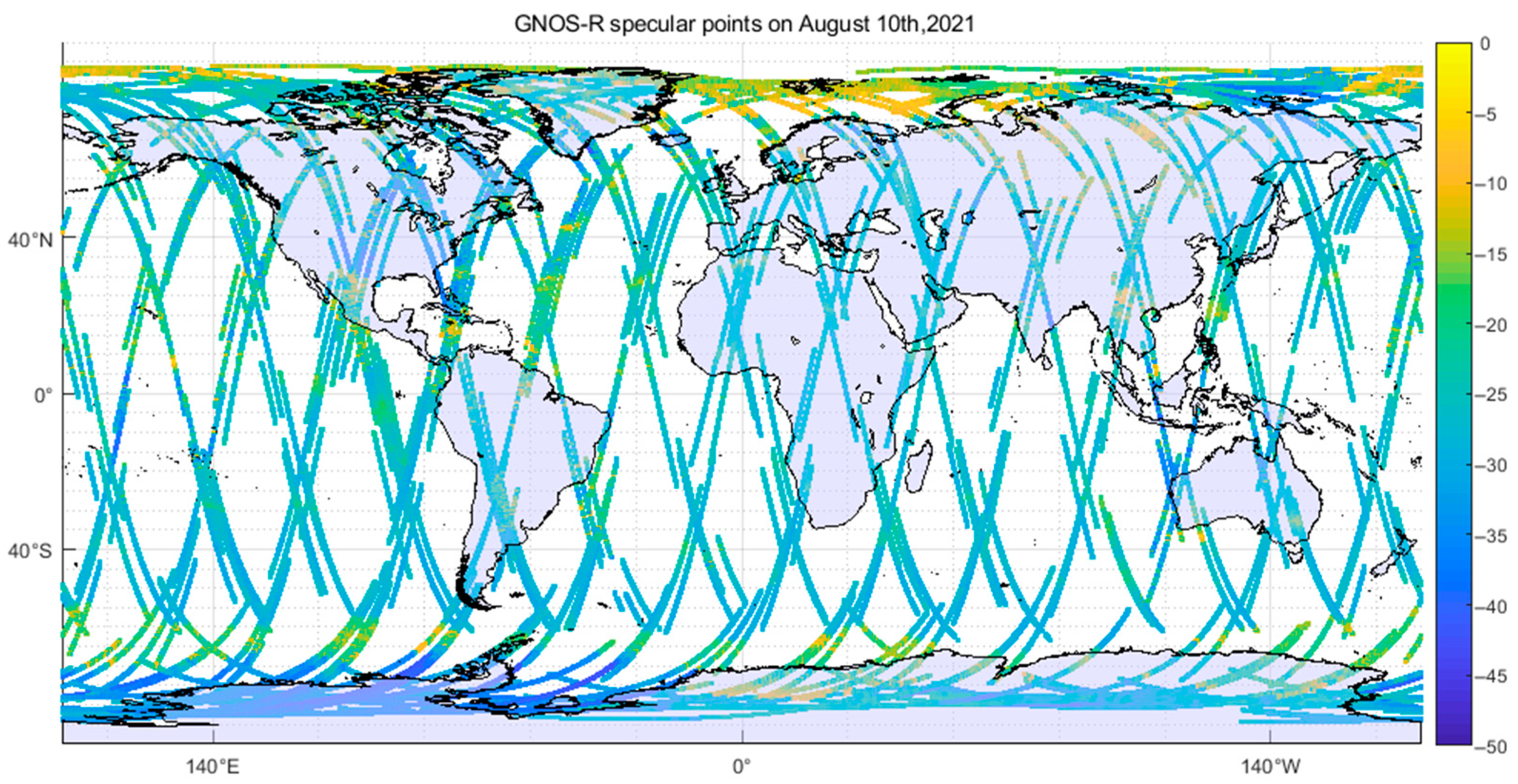
2.1. FY-3E GNOS-R Dataset
2.2. Ancillary Data from SMAP
2.3. Land Cover and Land Type Classification
3. Methodology
3.1. Bare Soil Formula and Simulations
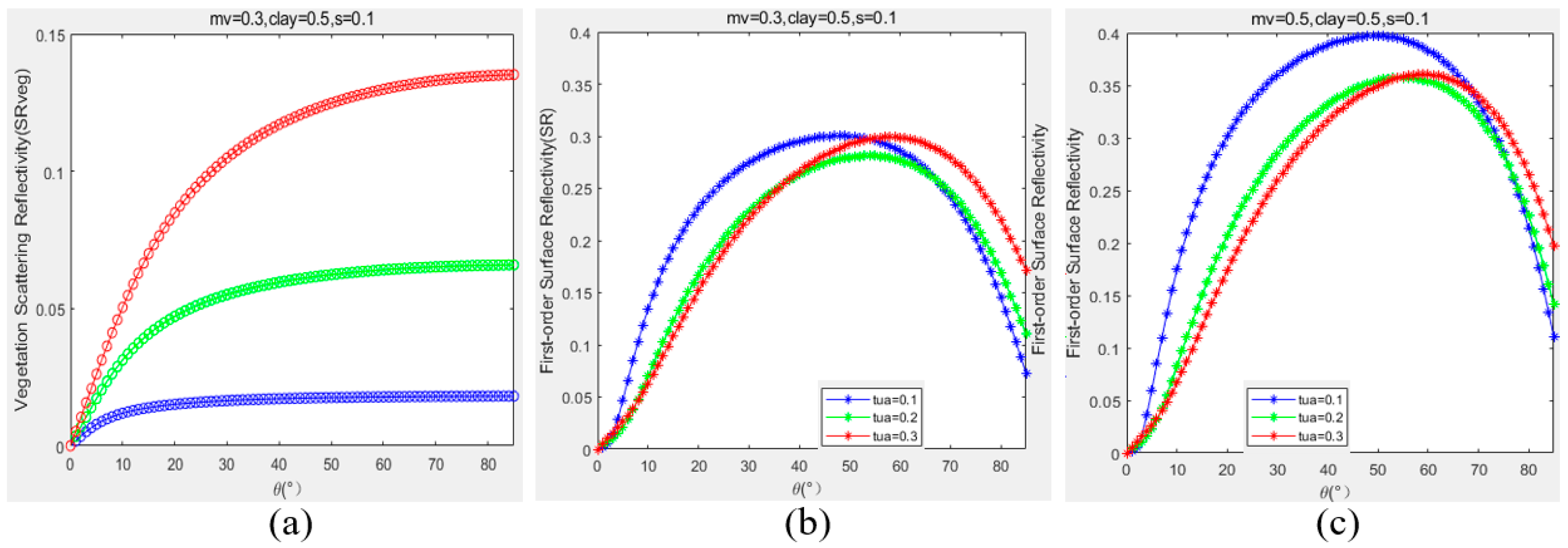
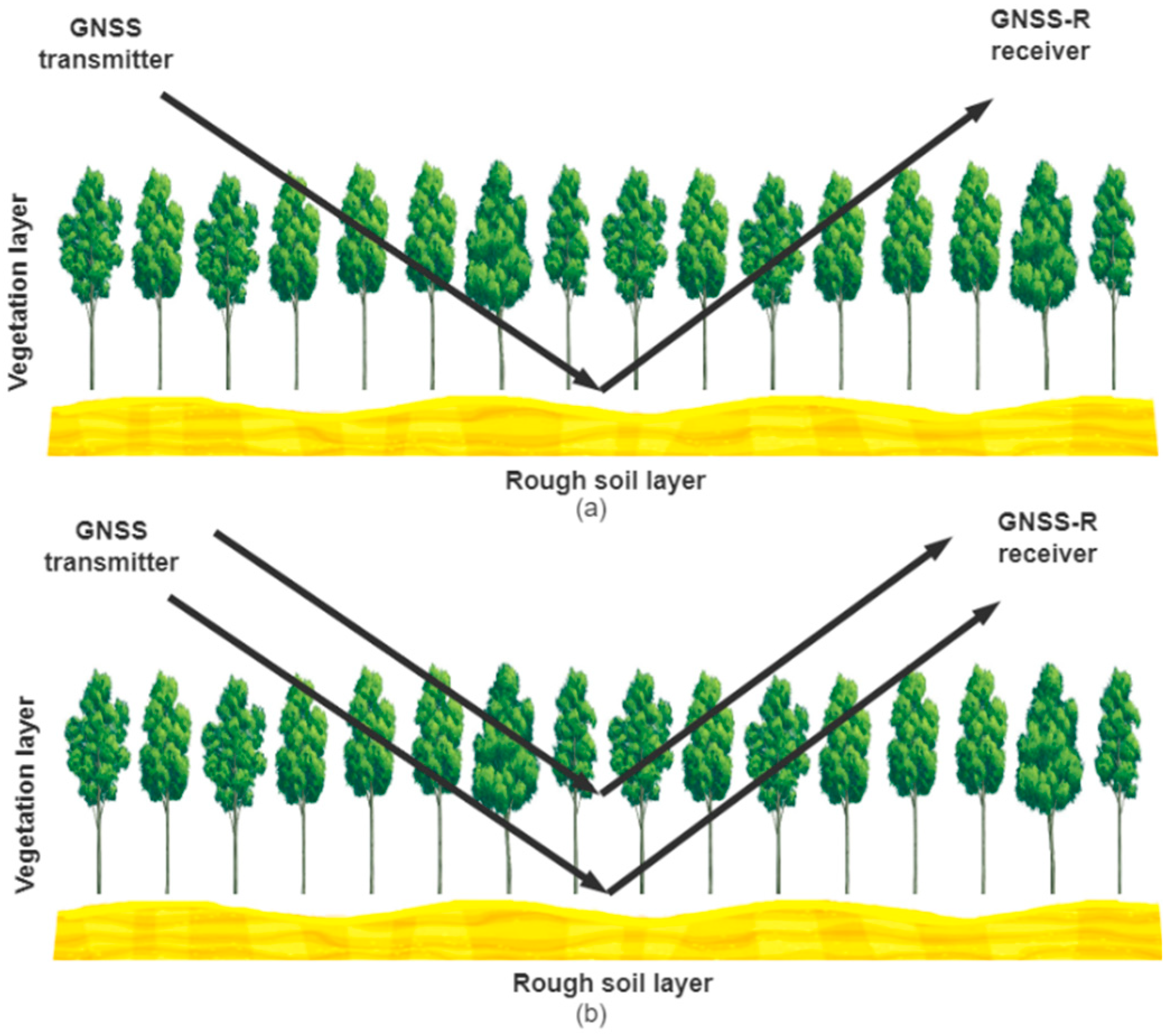
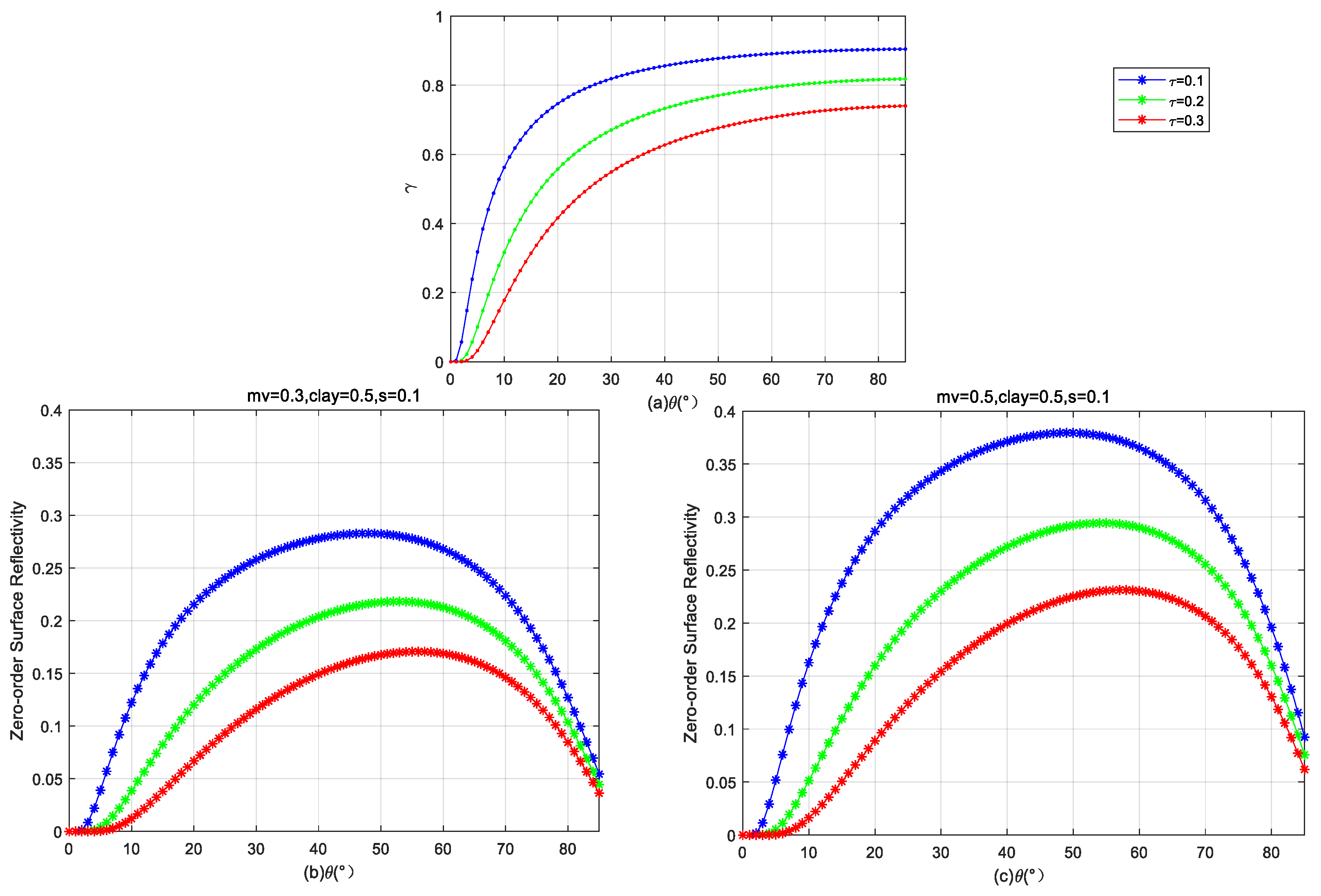
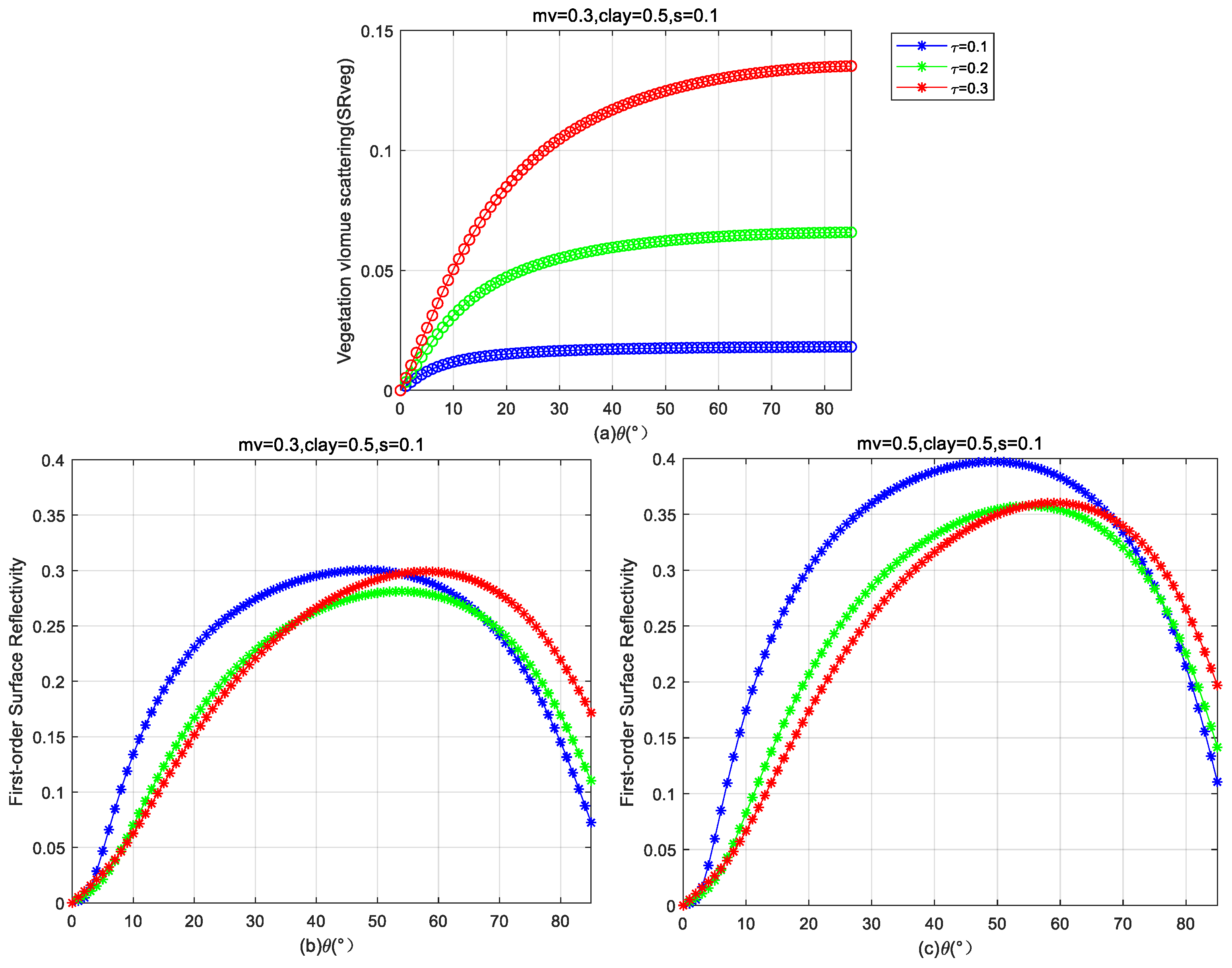
3.2. Vegetation Formula and Simulations
3.3. Soil Moisture Retrieval Algorithm
4. Results
4.1. Performance of SM Retrieval for Barren Land Type
4.2. Soil Moisture Retrieval in Low-Vegetation-Coverage Areas
4.3. Soil Moisture Retrieval for High-Forest-Coverage Areas
5. Conclusions
Author Contributions
Funding
Data Availability Statement
Conflicts of Interest
References
- Hall, C.; Cordey, R. Multistatic Scatterometry. In Proceedings of the International Geoscience and Remote Sensing Symposium (IGARSS), Edinburgh, UK, 13–16 September 1988; pp. 561–562. [Google Scholar] [CrossRef]
- Martin-Neira, M.A. A Passive Reflectometry and Interferometry System (PARIS): Application to Ocean Altimetry. ESA J. 1993, 17, 331–355. [Google Scholar]
- Zavorotny, V.U.; Gleason, S.; Cardellach, E.; Camps, A. Tutorial on Remote Sensing Using GNSS Bistatic Radar of Opportunity. IEEE Geosci. Remote Sens. Mag. 2014, 2, 8–45. [Google Scholar] [CrossRef]
- Yan, Q.; Huang, W.; Jin, S.; Jia, Y. Pan-Tropical Soil Moisture Mapping Based on a Three-Layer Model from CYGNSS GNSS-R Data. Remote Sens. Environ. 2020, 247, 111944. [Google Scholar] [CrossRef]
- Carreno-Luengo, H.; Luzi, G.; Crosetto, M. Above-Ground Biomass Retrieval over Tropical Forests: A Novel GNSS-R Approach with CyGNSS. Remote Sens. 2020, 12, 1368. [Google Scholar] [CrossRef]
- Chew, C.; Reager, J.T.; Small, E. CYGNSS Data Map Flood Inundation During the 2017 Atlantic Hurricane Season. Sci. Rep. 2018, 8, 9336. [Google Scholar] [CrossRef] [PubMed]
- Carreno-Luengo, H.; Ruf, C.S. Mapping Freezing and Thawing Surface State Periods with the CYGNSS-Based F/T Seasonal Threshold Algorithm. IEEE J. Sel. Top. Appl. Earth Obs. Remote Sens. 2022, 15, 9943–9952. [Google Scholar] [CrossRef]
- Gleason, S.; Adjrad, M.; Unwin, M. Sensing Ocean, Ice and Land Reflected Signals from Space: Results from the UK-DMC GPS Reflectometry Experiment. In Proceedings of the 18th International Technical Meeting of the Satellite Division of the Institute of Navigation (ION GNSS), Long Beach, CA, USA, 13–16 September 2005; pp. 1679–1685. [Google Scholar]
- Mashburn, J.; Axelrad, P.; Lowe, S.T.; Larson, K.M. Global Ocean Altimetry with GNSS Reflections from TechDemoSat-1. IEEE Trans. Geosci. Remote Sens. 2018, 56, 4088–4097. [Google Scholar] [CrossRef]
- Ruf, C.S.; Chew, C.; Lang, T.; Morris, M.G.; Nave, K.; Ridley, A.; Balasubramaniam, R. A New Paradigm in Earth Environmental Monitoring with the CYGNSS Small Satellite Constellation. Sci. Rep. 2018, 8, 8782. [Google Scholar] [CrossRef] [PubMed]
- Wan, W.; Liu, B.; Guo, Z.; Lu, F.; Niu, X.; Li, H.; Ji, R.; Cheng, J.; Li, W.; Chen, X.; et al. Initial Evaluation of the First Chinese GNSS-R Mission BuFeng-1 A/B for Soil Moisture Estimation. IEEE Geosci. Remote Sens. Lett. 2022, 19, 8017305. [Google Scholar] [CrossRef]
- Unwin, M.J.; Pierdicca, N.; Cardellach, E.; Rautiainen, K.; Foti, G.; Blunt, P.; Guerriero, L.; Santi, E.; Tossaint, M. An Introduction to the HydroGNSS GNSS Reflectometry Remote Sensing Mission. IEEE J. Sel. Top. Appl. Earth Obs. Remote Sens. 2021, 14, 6987–6999. [Google Scholar] [CrossRef]
- Sun, Y.; Huang, F.; Xia, J.; Yin, C.; Bai, W.; Du, Q.; Wang, X.; Cai, Y.; Li, W.; Yang, G.; et al. GNOS-II on Fengyun-3 Satellite Series: Exploration of Multi-GNSS Reflection Signals for Operational Applications. Remote Sens. 2023, 15, 5756. [Google Scholar] [CrossRef]
- Shi, J.; Dong, X.; Zhao, T.; Du, J.; Jiang, L.; Du, Y.; Liu, H.; Wang, Z.; Ji, D.; Xiong, C. WCOM: The Science Scenario and Objectives of a Global Water Cycle Observation Mission. In Proceedings of the IEEE International Geoscience and Remote Sensing Symposium (IGARSS), Quebec City, QC, Canada, 13–18 July 2014; pp. 3646–3649. [Google Scholar] [CrossRef]
- Zhao, T.; Shi, J.; Lv, L.; Xu, H.; Chen, D.; Cui, Q.; Jackson, T.J.; Yan, G.; Jia, L.; Chen, L.; et al. Soil Moisture Experiment in the Luan River Supporting New Satellite Mission Opportunities. Remote Sens. Environ. 2020, 240, 111680. [Google Scholar] [CrossRef]
- Entekhabi, D.; Njoku, E.G.; O’Neill, P.E.; Kellogg, K.H.; Crow, W.T.; Edelstein, W.N.; Entin, J.K.; Goodman, S.D.; Jackson, T.J.; Johnson, J.; et al. The Soil Moisture Active Passive (SMAP) Mission. Proc. IEEE 2010, 98, 704–716. [Google Scholar] [CrossRef]
- Chew, C.C.; Small, E.E. Soil Moisture Sensing Using Spaceborne GNSS Reflections: Comparison of CYGNSS Reflectivity to SMAP Soil Moisture. Geophys. Res. Lett. 2018, 45, 4049–4057. [Google Scholar] [CrossRef]
- Kim, H.; Lakshmi, V. Use of Cyclone Global Navigation Satellite System (CyGNSS) Observations for Estimation of Soil Moisture. Geophys. Res. Lett. 2018, 45, 8272–8282. [Google Scholar] [CrossRef]
- Clarizia, M.P.; Pierdicca, N.; Costantini, F.; Floury, N. Analysis of CYGNSS Data for Soil Moisture Retrieval. IEEE J. Sel. Top. Appl. Earth Obs. Remote Sens. 2019, 12, 2227–2235. [Google Scholar] [CrossRef]
- Yang, G.; Du, X.; Huang, L.; Wu, X.; Sun, L.; Qi, C.; Zhang, X.; Wang, J.; Song, S. An Illustration of FY-3E GNOS-R for Global Soil Moisture Monitoring. Sensors 2023, 23, 5825. [Google Scholar] [CrossRef] [PubMed]
- NASA EOSDIS Land Processes DAAC. MODIS/Terra+Aqua Land Cover Type Yearly L3 Global 0.05Deg CMG (MCD12C1). Available online: https://doi.org/10.5067/MODIS/MCD12C1.006 (accessed on 6 October 2022).
- Choudhury, B.J.; Schmugge, T.J.; Chang, A.; Newton, R.W. Effect of Surface Roughness on the Microwave Emission from Soils. J. Geophys. Res. 1979, 84, 5699–5706. [Google Scholar] [CrossRef]
- Bindlish, R.; Barros, A.P. Parameterization of Vegetation Backscatter in Radar-Based Soil Moisture Estimation. Remote Sens. Environ. 2001, 76, 130–137. [Google Scholar] [CrossRef]


| Name | Value | New Classifications |
|---|---|---|
| Evergreen Needleleaf Forests | 1 | Forest |
| Evergreen Broadleaf Forests | 2 | Forest |
| Deciduous Needleleaf Forests | 3 | Forest |
| Deciduous Broadleaf Forests | 4 | Forest |
| Mixed Forests | 5 | Forest |
| Closed Shrublands | 6 | Forest |
| Open Shrublands | 7 | Low-Vegetation |
| Woody Savannas | 8 | Low-Vegetation |
| Savannas | 9 | Low-Vegetation |
| Grasslands | 10 | Low-Vegetation |
| Permanent Wetlands | 11 | Low-Vegetation |
| Croplands | 12 | Low-Vegetation |
| Urban and Built-up Lands | 13 | Abandoned-type |
| Cropland/Natural Vegetation Mosaics | 14 | Low-Vegetation |
| Permanent Snow and Ice | 15 | Abandoned-type |
| Barren | 16 | Barren |
| Water Bodies | 17 | Abandoned-type |
| Unclassified | 255 | Abandoned-type |
| Observation Geometry θ | Case 1 | Case 2 |
|---|---|---|
| 0–10° | 1.4–4 | 1.5–11 |
| 11–20° | 2.1–4.5 | 2.1–12 |
| 21–30° | 2.2–4.8 | 2.2–13 |
| 31–40° | 2.2–5.5 | 2.2–14 |
| 41–50° | 2.5–5.5 | 2.5–14.5 |
| >50° | 3–5.5 | 4–14.1 |
| Incidence Angles θ | RMSE (Case 1) | RMSE (Case 2) |
|---|---|---|
| 0–10° | 0.0061 | 0.0057 |
| 11–20° | 0.0259 | 0.0252 |
| 21–30° | 0.0245 | 0.0205 |
| 31–40° | 0.0214 | 0.0161 |
| 41–50° | 0.0180 | 0.0111 |
| >50° | 0.0055 | 0.0048 |
| Combination considerations of incidence angles separation | 0.0235 | 0.0224 |
| Case 1 | Case 2 | Case 3 | Case 4 | |
|---|---|---|---|---|
| 0–10° | 0.0361 | 0.0447 | 0.0336 | 0.0440 |
| 11–20° | 0.0358 | 0.0390 | 0.0390 | 0.0410 |
| 21–30° | 0.0359 | 0.0330 | 0.0332 | 0.0331 |
| 31–40° | 0.0332 | 0.0300 | 0.0307 | 0.0283 |
| 41–50° | 0.0300 | 0.0261 | 0.0379 | 0.0340 |
| >50° | 0.0470 | 0.0301 | 0.0306 | 0.0310 |
| Combination considerations of incidence angles separation | 0.0296 | 0.0290 | 0.0305 | 0.0316 |
| Case 1 | Case 2 | Case 3 | Case 4 | |
|---|---|---|---|---|
| 0–10° | 0.0288 | 0.0381 | 0.0258 | 0.0380 |
| 11–20° | 0.0280 | 0.0323 | 0.0273 | 0.0322 |
| 21–30° | 0.0278 | 0.0212 | 0.0260 | 0.0253 |
| 31–40° | 0.0236 | 0.0193 | 0.0244 | 0.0198 |
| 41–50° | 0.0197 | 0.0218 | 0.0251 | 0.0245 |
| >50° | 0.0315 | 0.0316 | 0.0315 | 0.0317 |
| Final accuracy | 0.0195 | 0.0191 | 0.0215 | 0.0222 |
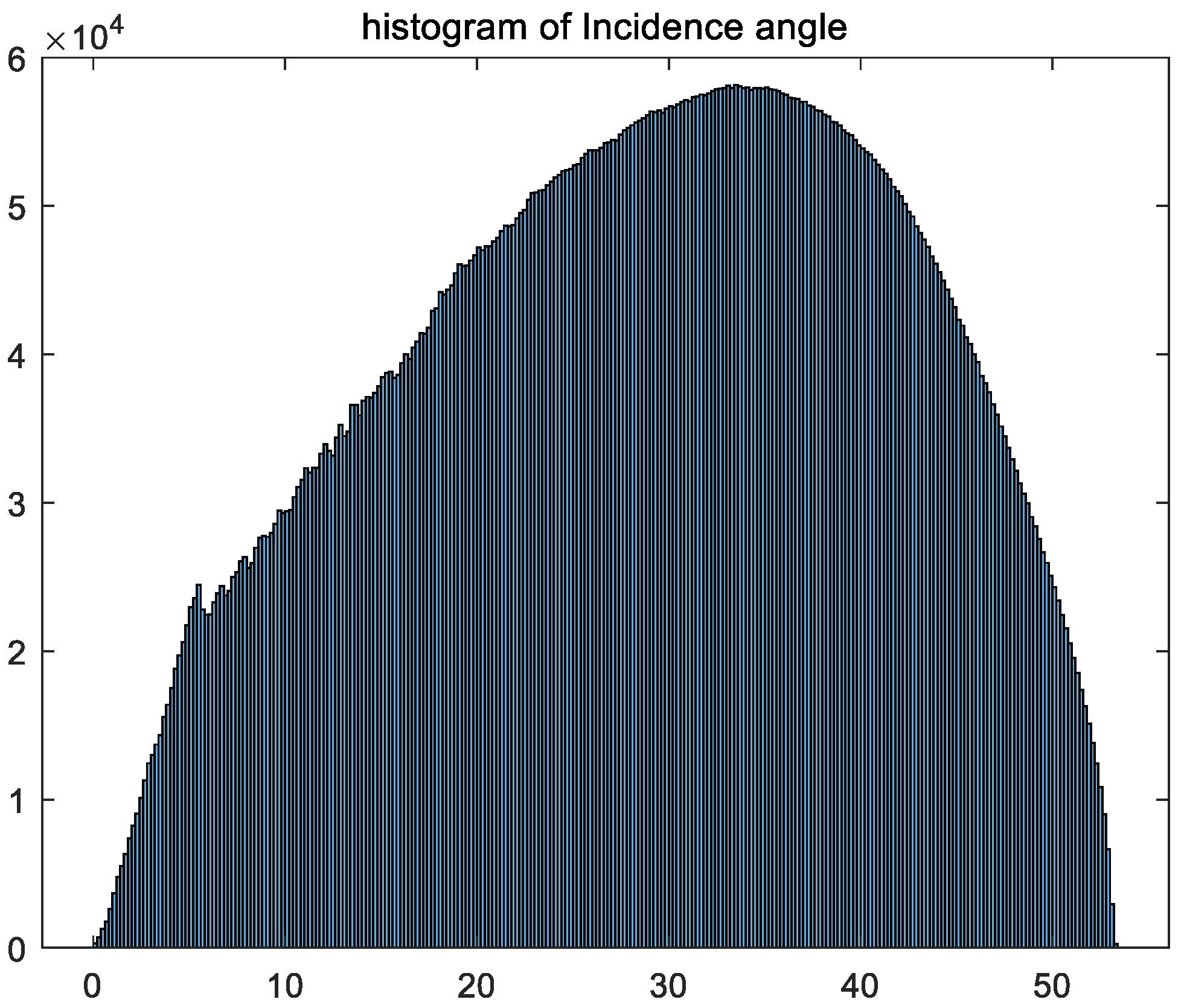
| Specular Incidence Angles | Percentage |
|---|---|
| 0–10° | 8.43% |
| 11–20° | 17.97% |
| 21–30° | 24.66% |
| 31–40° | 26.87% |
| 41–50° | 19.67% |
| >50° | 2.40% |
Disclaimer/Publisher’s Note: The statements, opinions and data contained in all publications are solely those of the individual author(s) and contributor(s) and not of MDPI and/or the editor(s). MDPI and/or the editor(s) disclaim responsibility for any injury to people or property resulting from any ideas, methods, instructions or products referred to in the content. |
© 2025 by the authors. Licensee MDPI, Basel, Switzerland. This article is an open access article distributed under the terms and conditions of the Creative Commons Attribution (CC BY) license (https://creativecommons.org/licenses/by/4.0/).
Share and Cite
Wu, X.; Xia, J.; Bai, W.; Sun, Y. Advancing GNOS-R Soil Moisture Estimation: A Multi-Angle Retrieval Algorithm for FY-3E. Remote Sens. 2025, 17, 2325. https://doi.org/10.3390/rs17132325
Wu X, Xia J, Bai W, Sun Y. Advancing GNOS-R Soil Moisture Estimation: A Multi-Angle Retrieval Algorithm for FY-3E. Remote Sensing. 2025; 17(13):2325. https://doi.org/10.3390/rs17132325
Chicago/Turabian StyleWu, Xuerui, Junming Xia, Weihua Bai, and Yueqiang Sun. 2025. "Advancing GNOS-R Soil Moisture Estimation: A Multi-Angle Retrieval Algorithm for FY-3E" Remote Sensing 17, no. 13: 2325. https://doi.org/10.3390/rs17132325
APA StyleWu, X., Xia, J., Bai, W., & Sun, Y. (2025). Advancing GNOS-R Soil Moisture Estimation: A Multi-Angle Retrieval Algorithm for FY-3E. Remote Sensing, 17(13), 2325. https://doi.org/10.3390/rs17132325