Abstract
The Very Long Baseline Interferometry Global Observing System (VGOS), a global network of stations equipped with small-diameter, fast-slewing antennas and broadband receivers, is primarily utilized for geodesy and astrometry. In China, the Shanghai and Urumqi VGOS stations have been developed to perform radio source observation regularly. However, these VGOS stations have not yet been used to observe Earth satellites or deep-space probes. In addition, suitable systems for processing VGOS satellite data are unavailable. In this study, we explored a data processing pipeline and method suitable for VGOS data observed in the dual linear polarization mode and applied to the differential observation of satellites. We present the VGOS observations of the Chang’e 5 lunar orbiter as a pilot experiment for VGOS observations of Earth satellites to verify our processing pipeline. The interferometric fringes were obtained by the cross-correlation of Chang’e 5 lunar orbiter signals. The data analysis yielded a median delay precision of 0.16 ns with 30 s single-channel integration and a baseline closure delay standard deviation of 0.14 ns. The developed data processing pipeline can serve as a foundation for future Earth-orbiting satellite observations, potentially supporting space-tie satellite missions aimed at constructing the terrestrial reference frame (TRF).
1. Introduction
Very long baseline interferometry (VLBI) is a space geodetic technique. However, the legacy VLBI systems developed 30 years ago have precision limitations and are difficult to maintain. As such, a new generation VLBI Global Observing System (VGOS) was developed to provide highly precise data products, including station positions and Earth orientation parameters (EOP) [1]. A VGOS antenna has a smaller aperture, faster antenna slewing rate, and super-wide bandwidth with dual linear polarization [2], which allows for the acquisition of more observations and precise delay observables. Moreover, it has the potential to observe fast-moving Earth-orbiting satellites.
The International Terrestrial Reference Frame (ITRF) is a combined product of four space geodetic techniques: VLBI, Satellite Laser Ranging (SLR), the Global Navigation Satellite System (GNSS), and Doppler Orbitography and Radiopositioning Integrated by Satellite (DORIS) [3]. The long-term origin positional accuracy of the ITRF2020 is 5 mm [3], primarily attributable to the accuracy of the linking measurement and systematic errors of the individual techniques. A newly proposed approach involves using space ties, in which multiple space geodetic techniques are co-located on the same satellite to improve the accuracy of geodetic measurements. These include analyses of the Jason-2 satellite involving GNSS, SLR, and DORIS for the co-location of low Earth orbit (LEO) satellites within the TRF framework [4]; the combination of geodetic observation techniques onboard satellites for the improvements needed to realize a long-term accurate and stable TRF [5]; and the realization of space ties and co-location of four space geodetic techniques on one satellite in GENESIS, establishing a precise and stable combination among key space geodetic techniques [6].
Numerous simulations and experiments have been conducted on space ties with VLBI. Plank et al. [7] conducted simulations and explored the potential of VLBI satellite tracking for establishing frame ties. Anderson et al. [8] simulated VLBI observations of a space-tie satellite. Klopotek et al. [9] explored a feasibility study on using geodetic VLBI for precise orbit determination of Earth satellites. Schunck et al. [10] conducted simulations of VLBI observations to BeiDou and Galileo satellites to establish frame ties. However, a fundamental issue with combining space geodetic techniques is the absence of actual satellite observations with VLBI antennas and the lack of a well-established data processing chain for establishing frame ties using Earth satellites. Consequently, researchers have conducted VLBI observation experiments on the APOD satellite using the AuScope array and developed a procedure chain aimed at space-tie satellite missions for ITRF [11,12]. Plank et al. [13] performed experiments to observe GNSS satellites using the Hobart and Ceduna VLBI stations in Australia. The developed processing chain has the potential to be applied to observe space-tie satellites. Schunck et al. [14] explored the VLBI observations of GENESIS in global VGOS network operations, to determine the realistic observability of both geodetic radio sources and GENESIS. To date, most space-tie satellite observations have been conducted with legacy VLBI antennas; however, few experiments have been conducted with VGOS.
China has considerable experience in VLBI observations for deep-space exploration, including the lunar and Mars series of missions [15,16,17]. However, no experiments have been conducted in China employing VGOS to observe Earth satellites. Three VGOS antennas (SESHAN13 and TIANMA13 at Shanghai, and URUMQI13 at Urumqi) are operational in China with the first broadband fringe of SESHAN13 and URUMQI13 obtained in 2020. Since then, the VGOS stations have participated in international VGOS observations and UT1 intensives within the International VLBI Service for Geodesy and Astrometry (IVS) [18].
VGOS feed horns are linearly polarized, so we record the circularly polarized signal from the satellite in two polarizations at each station. During correlation, the two polarization data streams from each station are cross-correlated, resulting in four correlation products, i.e., XX, XY, YX, and YY. In stark contrast to the approach by McCallum et al. [19] using only the XX product, all subsequent data processing in our work uses XX, XY, YX, and YY products; the combination and calibration of full polarization data present significant challenges to data processing techniques. Several studies have investigated classic VLBI tracking of satellites using legacy antennas (e.g., VLBA or the Deep Space Network) at the S, X, or Ka band in circular polarization [16,17,20]. However, this study employs small-antenna satellite observations in dual linear polarization and ultra-wideband mode. Thus, the methodology in the two cases is quite different.
In the Chinese VLBI Network (CVN), the data processing system serves as a conventional legacy S/X VLBI correlator, primarily used for the differential VLBI observation data processing of spacecraft tracking. The DiFX [21] software correlator specializes in astronomical and geodetic data correlation processing. However, for our data processing, the following limitations exist:
- The legacy S/X VLBI data processing system is incapable of processing VGOS data because of the different data format and polarization;
- Domestic DiFX implementations currently lack adequate satellite signal processing capabilities owing to access restrictions.
To address these limitations, we have independently developed a dedicated data processing pipeline suitable for VGOS data observed in the dual linear polarization mode of satellites.
We verified the effectiveness of our data processing pipeline by conducting VGOS observations of the Chang’e 5 lunar orbiter as a pilot experiment for VGOS observations of Earth satellites. The data processing quality proof includes suitable strategies for dealing with the satellite signal and the various polarization products, as well as group residual delays and delay precision in the fringe fitting procedures. Section 2 provides an overview of the VGOS observation experiment conducted in this study. Section 3 presents the data processing pipeline and method for VGOS data observed in the dual linear polarization mode. Section 4 outlines the data analysis and results, which are then discussed along with future research directions in Section 5.
2. Overview of the Observation Experiment
The Chinese Chang’e 5 lunar exploration mission has been equipped with VLBI transmitter and launched on 24 November 2020. The strength and bandwidth of the Chang’e 5 signals are more in line with the requirements of VGOS observation, and we have actual orbital information. Consequently, our experiment focused on the Chang’e 5 lunar orbiter. The observation of Earth satellites is planned for the future.
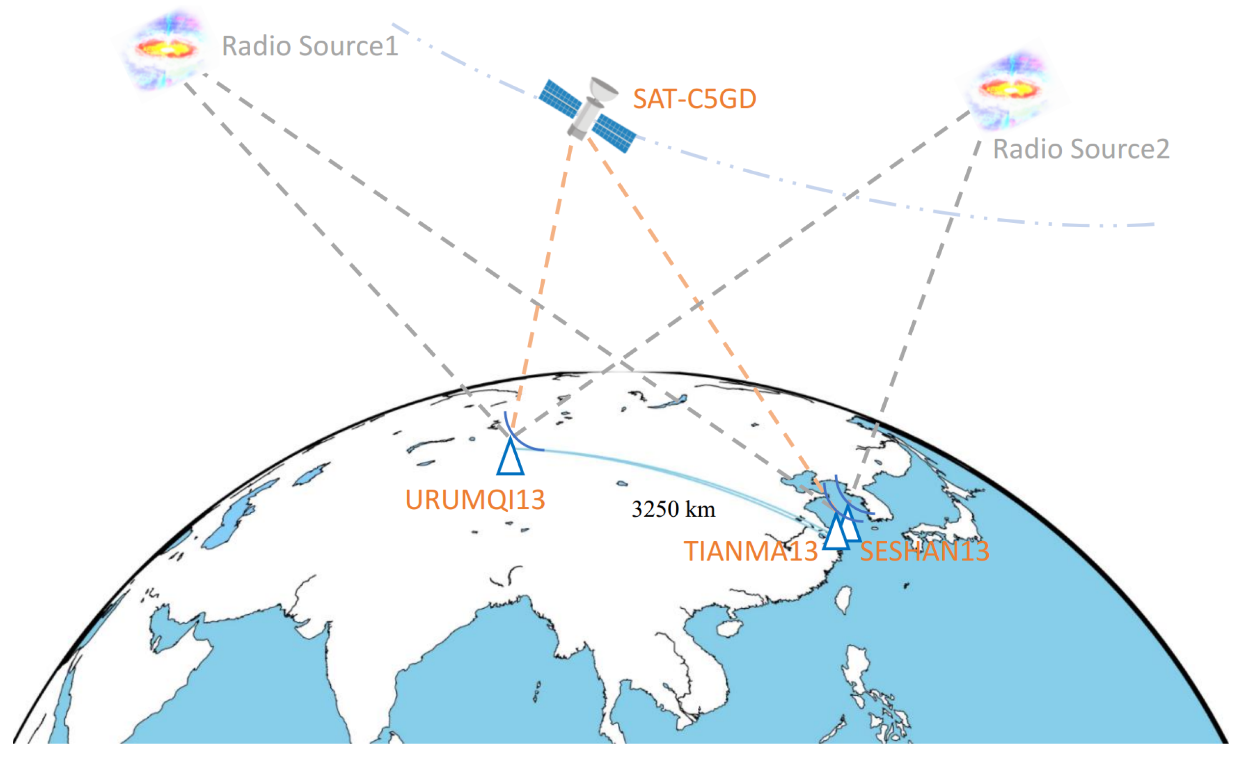
The experiment described herein was conducted using the Chinese VGOS stations SESHAN13, TIANMA13, and URUMQI13, as listed in Table 1. The longest baseline of approximately 3250 km is between the SESHAN13 and URUMQI stations, and the shortest baseline of approximately 6 km is between the SESHAN13 and TIANMA13 stations. Both stations are equipped with broadband receivers to receive dual linear polarized signals, Chinese VLBI Data Acquisition System (CDAS-2) backends, MARK6 recorder systems, and hydrogen atomic clocks for time synchronization. The VGOS Delta-Differential One-way Ranging (Delta-DOR) experiment was performed on 28 April 2023, from 05:10 to 06:40 UT. The experiment code was t3428m, and the observation geometry is shown in Figure 1. The Chang’e 5 lunar orbiter (SAT-C5GD) and the nearby radio sources (0552+398 (Radio Source1) and 0738+313 (Radio Source2)) as calibrators were observed alternately.

Table 1.
Chinese VGOS station characteristics.

Figure 1.
Schematic of the observation experiment.
The observations were performed at a 512 Mbps data rate, with four intermediate frequency (IF) channels and 2-bit sampling. Because VGOS observations need dual linear polarization, two IF channels were used for horizontal polarization (X), and the other two channels were used for vertical polarization (Y). Each IF channel had a bandwidth of 32 MHz (fixed for VGOS) with 64 Msps sampling. The raw data were recorded in the MARK6 system in VDIF format. The scan duration of the radio sources and satellite in this experiment ranged from 240 to 600 s.
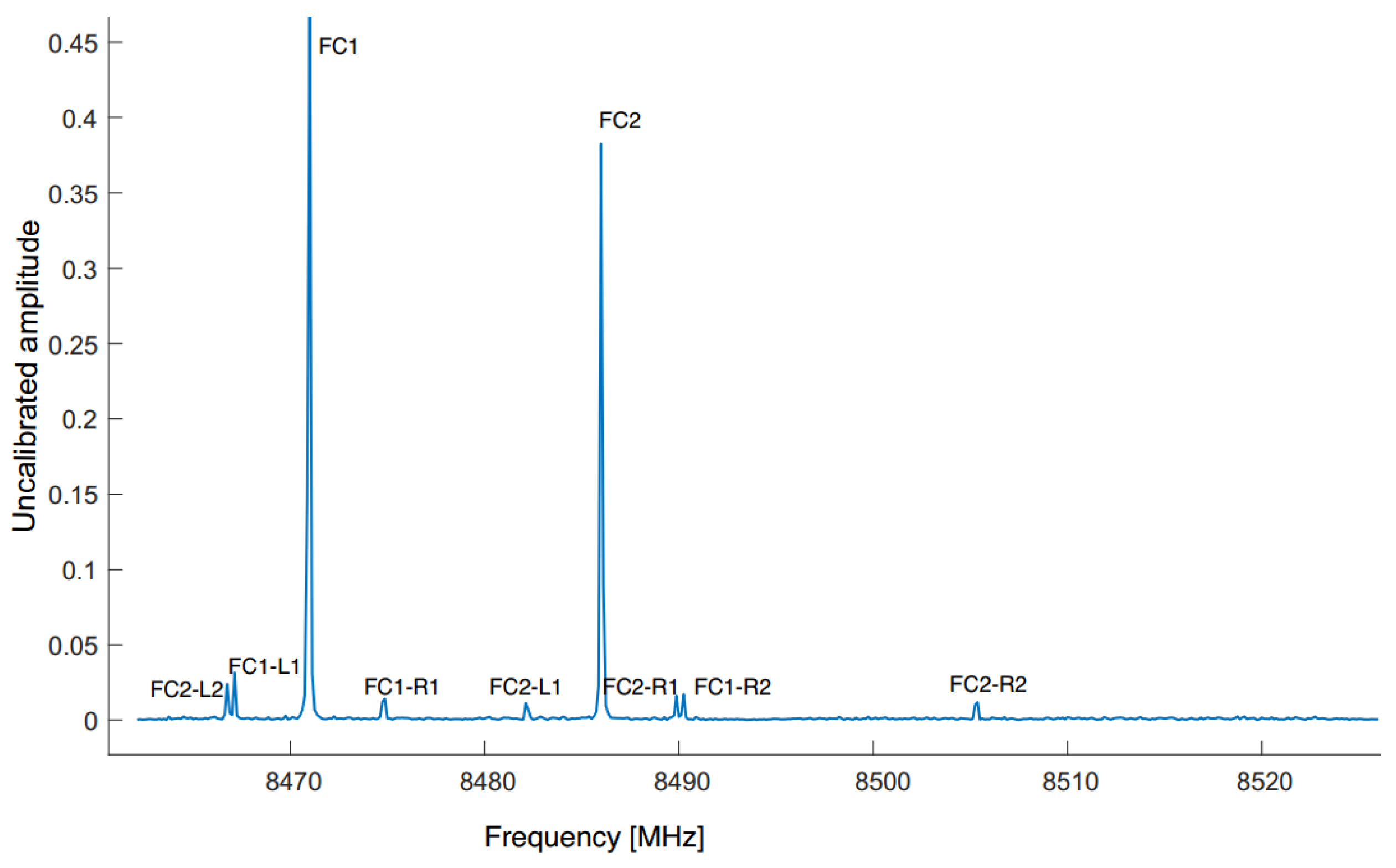
The Chang’e 5 lunar orbiter is equipped with several VLBI beacons. Two DOR beacon carriers centered on FC1 = 8471 MHz and FC2 = 8486 MHz. Only one carrier was used during data processing, with the other as a backup. As shown in Figure 2, the distribution of the DOR signals was derived from SAT-C5GD observation data. Each DOR has one carrier and four DOR tones designed in accordance with the recommendations of the Consultative Committee for Space Data Systems [22]. The DOR tones R1 (the right tone, e.g., FC1-R1, FC2-R1) and L1 (the left tone, e.g., FC1-L1, FC2-L1) are the first DOR tones, and R2 and L2 are the second DOR tones. The frequencies of the first and second DOR tones are calculated as DOR1 = FC ± FC/2200 and DOR2 = FC ± FC/440.

Figure 2.
Distribution of the observed DOR tones for the experiment.
3. Data Processing
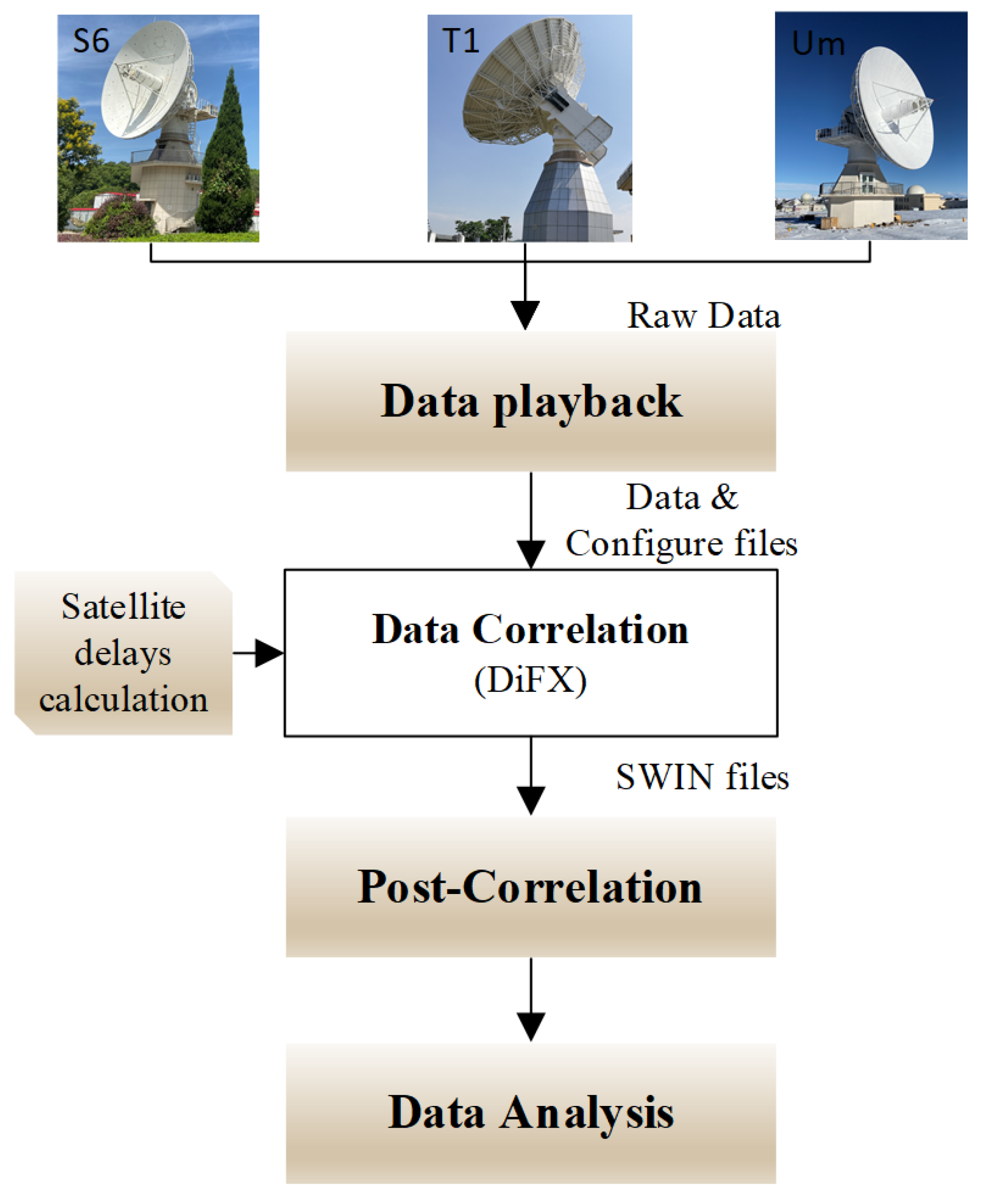
As illustrated in Figure 3, the observational data underwent a series of processing steps. The stations are responsible for conducting observations and recording and transferring the raw data. The raw observed data were transferred to the Shanghai VLBI Correlator for subsequent processing. The data processing included raw-data playback, correlation and post-processing, analysis, and other related processing. The modules contained within the pink boxes in Figure 3 were developed by the authors of this study.
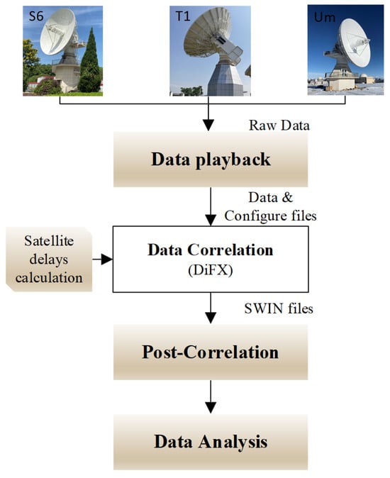
Figure 3.
Data processing workflow diagram.
3.1. Data Playback
The objective of VGOS data playback is to facilitate the pre-processing of received baseband data via reading, gathering, de-threading, and rebuilding steps. Data gathering involves extracting and combining raw data that have been scattered over multiple disks (16, 24, or 32) into a single ordered data group. In data de-threading, multiple threads and channel data are transformed into single-threaded baseband data with multiple- or single-channel configurations. After de-threading, if the data still have multiple IF channels, data rebuilding is necessary to convert them into a single multi-channel stream. For details on raw data playback, please refer to Gan et al. [23]. Upon completing the data playback, a list of files can be generated for subsequent data correlation.
3.2. Data Correlation
We employed standard correlator DiFX v2.5.5 [21] software for observational data correlation. The DiFX performed FX type data correlation, which included delay tracking, fringe stopping, fast Fourier transform (FFT), fractional bit correction, cross-multiplication, and long-term integration, to obtain the auto-correlation and cross-correlation spectra, i.e., the complex visibility function, which was saved in SWIN files [21]. The method and steps for satellite data correlation are the same as those of the radio sources. The primary distinction lies in the time-delay model.
The first step in the correlation procedure is establishing the time-delay model. We utilized the standard VLBI delay model in the DiFX software correlator for radio source signals.
Earth satellites are situated in the Earth’s near field, and the incoming wave fronts are regarded as spherical. Therefore, the standard VLBI delay model cannot be applied to satellite signals. In the study, we modeled a priori delay for satellite correlation. Pursuant to the observation schedule file, the program calculated the satellite delay model for each scan using the satellite ephemeris. Subsequently, fifth-order polynomials of the satellite delay model, valid in 30 s, were generated, along with the clock and clock rate. Finally, the polynomial coefficients were written into the input model files (IM files) of the DiFX correlator [21], which was employed to generate the requisite delay parameters for the Earth satellite correlation.
3.3. Data Post-Correlation
In the dual linear polarization mode, the post-correlation processing pipeline reads the SWIN files and performs multiple tasks—fringe fitting of cross-correlation spectra, delay/phase calibration, and polarization combination [24]—to generate fringe, delay, and delay precision results, among other outcomes.
3.3.1. Auto-Correlation
The satellite signal must be clearly identified for processing the cross-correlation spectra. The data should be repeatedly processed based on the strength of the satellite signal and bandwidth in order to select an appropriate spectral resolution for accurate identification of the signal. Therefore, autocorrelation data was extracted and analyzed during the post-correlation process to obtain the effective spectral resolution. Subsequently, we returned to using the correlator for correlation processing again with the identified FFT size from the spectral resolution.
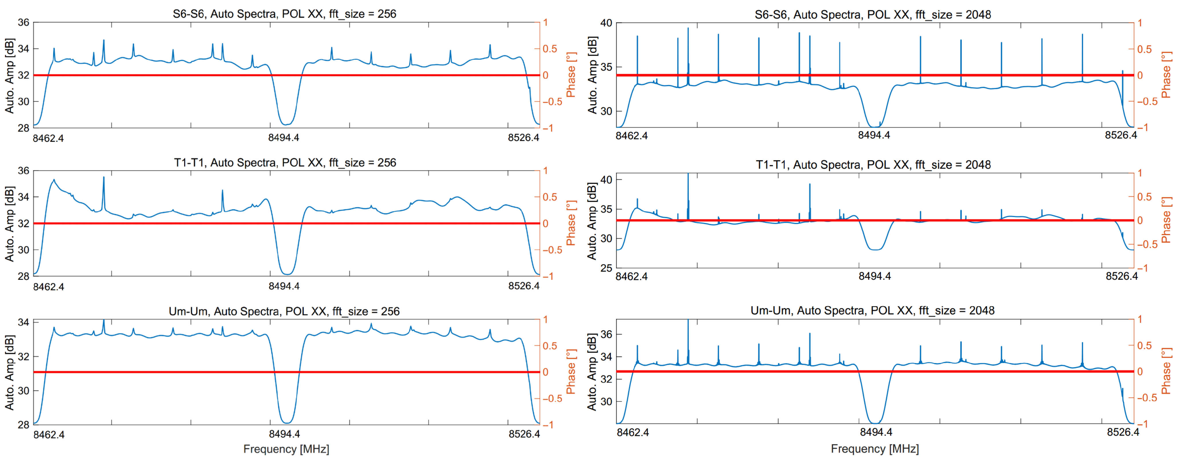
Figure 4 shows the magnitude-phase of the auto-correlation spectra of the three VGOS antennas, with two channels (Channel 1, 8462.4–8494.4 MHz; Channel 2, 8494.4–8526.4 MHz), and two polarization products (XX and YY). The figure shows the XX polarization spectra, which contains satellite (DOR) and phase calibration signals. The graphs in the left column were generated using an FFT size of 256 for correlation. The DOR signal magnitudes in the FFT size of 256 were relatively weak in Channel 1 and almost indistinguishable in Channel 2. For all antennas, only two carriers, FC1 and FC2, could be discerned, because the other DOR tones were obscured by baseband noise. The right column presents the auto-correlation spectra obtained following correlation with an FFT size of 2048. The magnitudes of FC1, FC2, and all the DOR tones in the channels were much larger and more identifiable compared with the magnitudes in the FFT size of 256. Accordingly, radio sources and SAT-C5GD scans were correlated at a fine spectral resolution of 15.6 kHz and a 2048 FFT size.
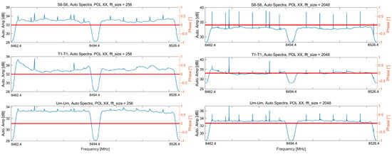
Figure 4.
Satellite auto-spectra magnitudes and phases for different FFT sizes. The left column is FFT size 256 and the right column is FFT size 2048. The horizontal axes indicate the frequency of each channel. The left vertical axes show the auto-spectra magnitudes, and the right vertical axes are the auto-spectra phases.
3.3.2. Cross-Correlation
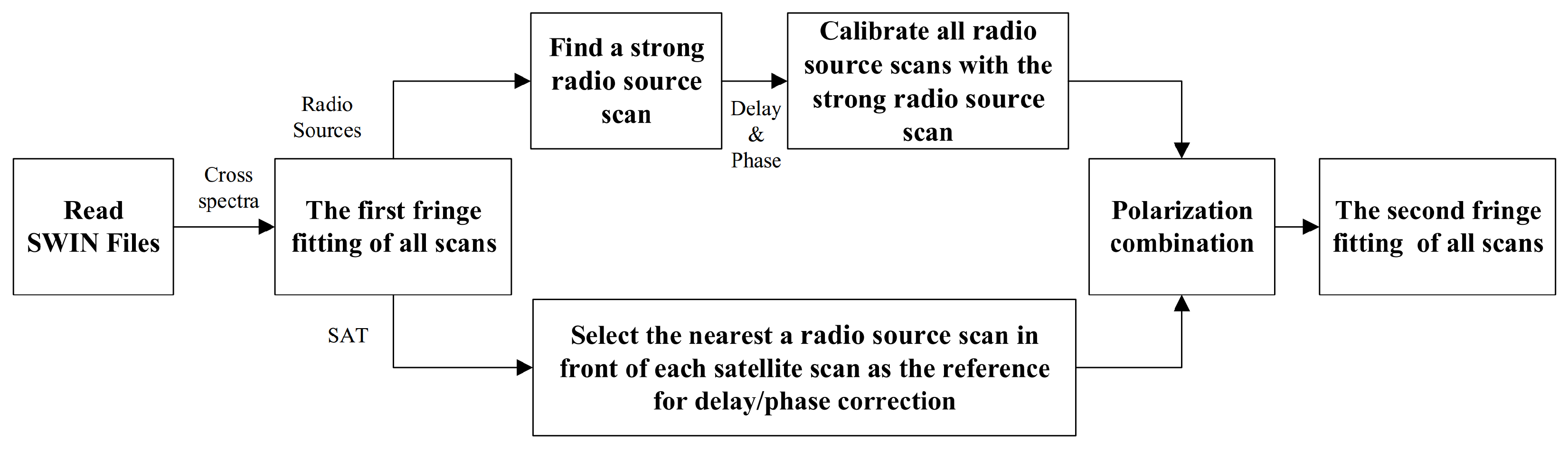
The cross-spectra of each scan comprise four polarization products: XX, YY, XY, and YX. Calibrating the delay and phase of each polarization product was necessary before combining the polarization products of each scan. Figure 5 shows the post-correlation processing for the cross-spectra. The details are as follows:
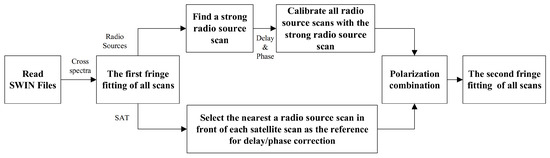
Figure 5.
Block diagram of post-correlation for the cross-correlation spectra.
- 1.
- Selection of fringe fitting data: All frequency point phases of each radio source scan were selected for processing. For each satellite scan, one carrier and its corresponding DOR tones frequency point phases were selected, thereby ensuring the maintenance of the phase variation rule. The experiment was processed for satellite scans using four frequency points of Channel 1, specifically FC1, FC1-L1, FC1-R1, and FC1-R2. The FC1-L2 of Channel 2 was not used, to avoid channel-to-channel delay.
- 2.
- Delay and phase calibration of the polarization products of scans: Following the first fringe fitting, the scan with a high SNR (≥30) on all polarization products was selected as the reference for the radio source signals. Calibrations were performed for all radio source scans using the delay and phase values from the reference scan. In the case of satellite scans, a radio source scan before the SAT-C5GD scan was used as the reference for delay and phase correction. In this experiment, no radio source was observed before the first SAT-C5GD scan. Therefore, the calibration for the first SAT-C5GD scan was performed with the radio source scan obtained subsequently.The experiment yielded three baselines: S6-Um, T1-Um, and S6-T1. A specialized calibration method was implemented to ensure the three-baseline residual time-delay closures. The symbols c, u, and t represent the S6, Um, and T1 stations, respectively. Using a radio source scan of the S6-Um baseline as an example, four polarization products (XcXu, YcYu, XcYu, and YcXu) were obtained after correlation. The X polarization of u was taken as the reference, i.e., the delay of () was set to zero (delay and phase were the same way; here, the delay calculation was used as an example). The X polarization delay of c () was obtained with the following:The Y polarization delay of c () was obtained with the following:Then, the Y polarization delay of u () was obtained withThese delay values were then used to correct the four polarization products of the S6-Um baseline, and the same strategy was used for phase calibration. The and (delay and phase) values of T1 were obtained from the T1-Um baseline using the same method, utilizing the X polarization of u as a reference, and the (delay/phase) values of u were not recalculated. The S6-T1 calibration values were calculated from the X and Y polarization delay/phase corresponding to c and t, which were obtained previously. is given as follows:Table 2 lists the delay/phase values used for calibration, corresponding to Channel 1 of each baseline for radio source No0009. The processing of XY/XX was unnecessary, given that the differential parallactic angle between stations S6 and T1 was essentially zero and the fringe of XY/YX was approximately non-existent.
Table 2. Delay and phase corresponding to the polarization products of the reference radio source (No0009) employed for calibration.
- 3.
- Polarization combination is the combination of four polarization products into a single Stokes-I observable [24] as follows:where a and b are two stations, and p is the differential parallactic angle between stations a and b. The polarization products are the data after delay and phase calibration in Step 2. For example, in this processing, was the time-averaged cross-spectra polarization product of the Y polarization of station a with the X polarization of station b. The information of all observed scans and differential parallactic angles are presented in Table 3.
Table 3. The particulars of the observation scans.
- 4.
- The fringe fitting employed the phase least-squares estimation, with the data phase obtained using the approach in Step 1. Fringe fitting was performed on the cross-correlation spectra of each polarization product and a combination of all scans. Subsequently, the residual delay and delay precision results were obtained.
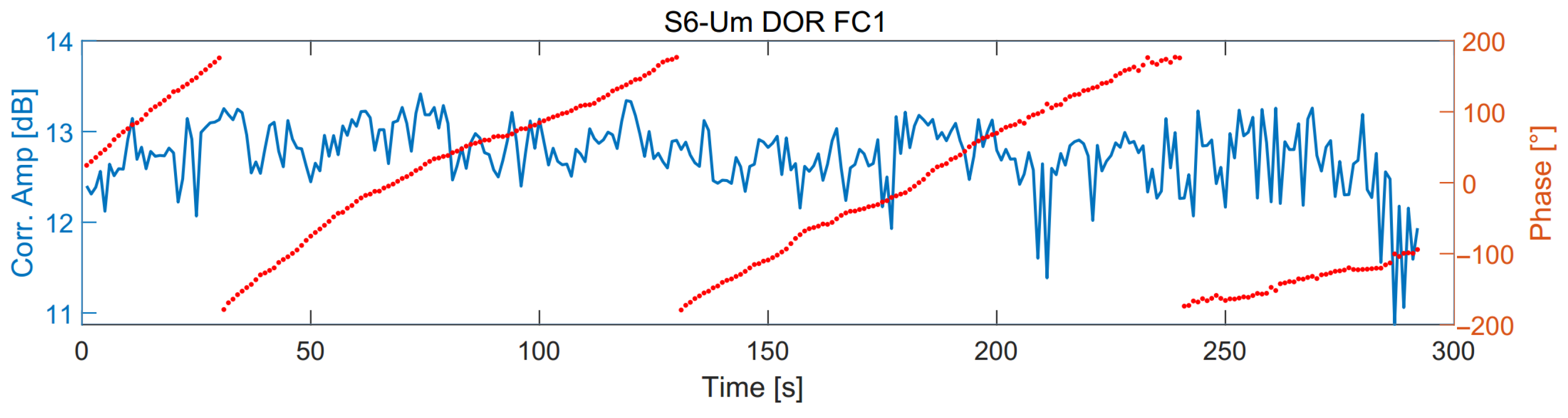
Following calibration, the satellite signal magnitude and phase in the time domain varied with time, as shown in Figure 6. The magnitude tended to vary over time. The phase could not maintain a linear change over time, making integration impossible over a long period.
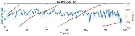
Figure 6.
Cross-spectra magnitudes (blue) and phases (red) of the carrier (FC1) of satellite scan No0008 in the time domain. The time axes (horizontal) indicate seconds since the start of scan No0008.
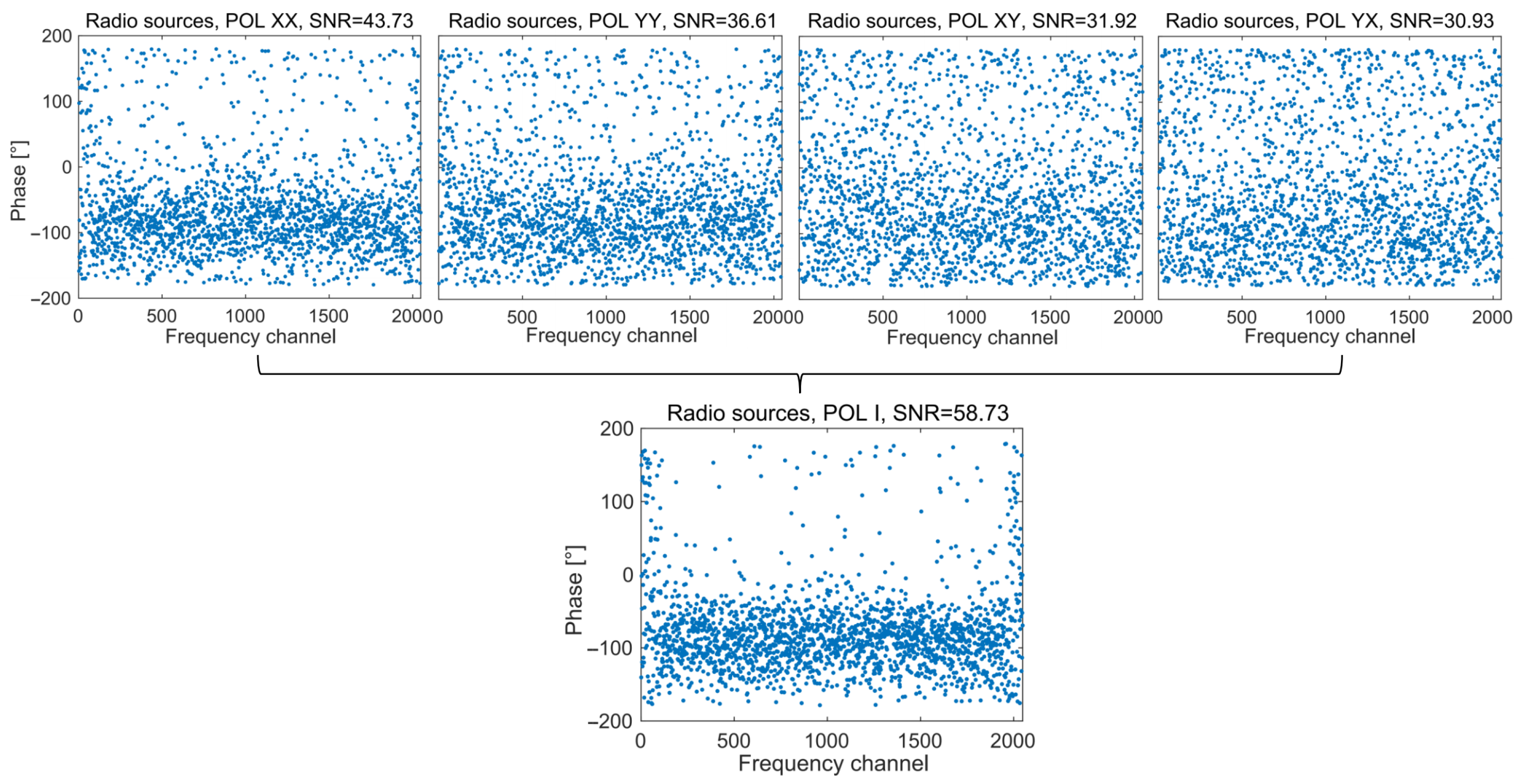
The polarization combination of radio source scan (No0009) is shown in Figure 7. As demonstrate in the upper four plots, the residual phase of the four polarization products ranges from to , and the SNR ranges from 30 to 44. The lower panel in Figure 7 reveals the fringes of the polarization combination; almost all the phases are concentrated within the range of to . The SNR improved by a factor of approximately 1.33 compared with XX (58.73). Polarization combination results are in a more focused phase, with significantly lower phase dispersion and improved delay measurement accuracy and SNR compared with the single-polarization products.
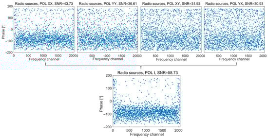
Figure 7.
Fringes of the radio source scan (No0009) polarization products and combination.
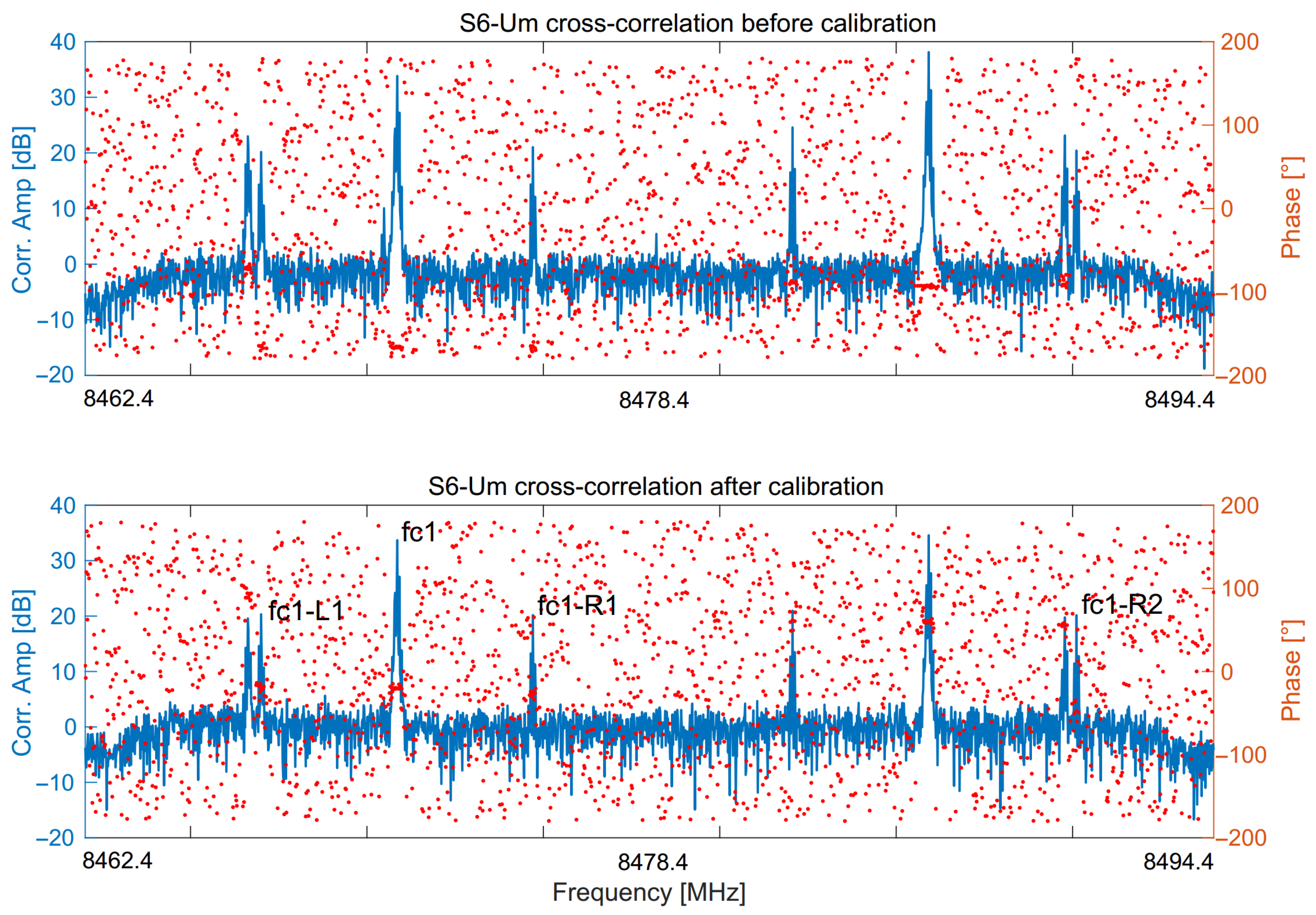
Figure 8 shows the SAT-C5GD fringes of the S6-Um baseline in the frequency domain. The upper panel shows the magnitude and phase plot before correlation processing, which reveals the disorder phases (red) of the DOR signals. The delay and phase calibration used for target signals effectively improved the baseline SNR, as evident from the phase in the lower panel of Figure 8. The phases within a narrow band of FC1, FC1-L1, FC1-R1, and FC1-R2 were aligned.
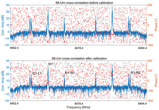
Figure 8.
Satellite cross-spectra (No0008, POL XX) magnitudes and phases in frequency series. The horizontal axes depict the channel frequency.
4. Results and Discussion
4.1. Results
The aforementioned data processing pipeline was used to perform delay and phase calibration, fringe fitting, and yield residual delays for the radio source and SAT-C5GD scans. We investigated the residual delays and delay precision for radio sources and the SAT-C5GD, respectively.
For radio sources, the relationship between single-channel delay precision and signal-to-noise ratio (SNR) is given as follows [25]:
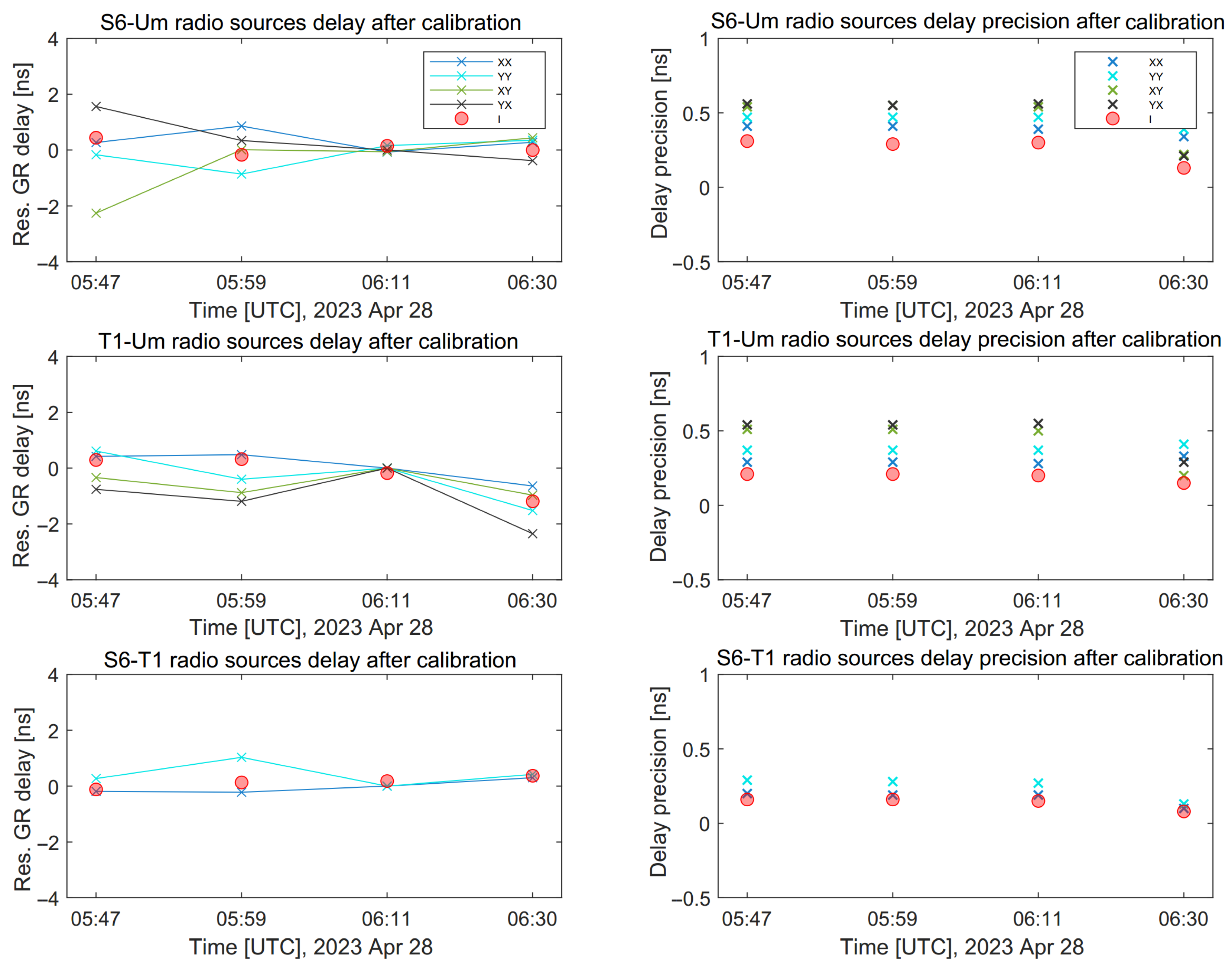
where is the delay precision, B is the bandwidth. The second fringe fitting of the radio source scans was performed on the XX/YY/XY/YX and I (see Figure 5). The integration times were the scan durations, as listed in Table 3. The residual delays and delay precision of the radio source scans for XX/YY/XY/YX and I are shown in Figure 9. The figure shows the residual delays for the three baselines (S6-Um, T1-Um, S6-T1) in the left column and the delay precision in the right column. The residual delays of XX/YY/XY/YX show variations of -4.50 to 3.00 ns over the scan duration. In contrast, the residual delays in the I are smaller, with variability near 0 ns. The delay precision values for XX/YY/XY/YX are in the 0.19–0.56 ns range. The delay precision values for I are in the range of 0.15–0.29 ns at an integration time of 300 s and 0.08–0.15 ns at 600 s for the three baselines. The delay precision is reduced in I, demonstrating that delay/phase calibration and polarization combination were effective.
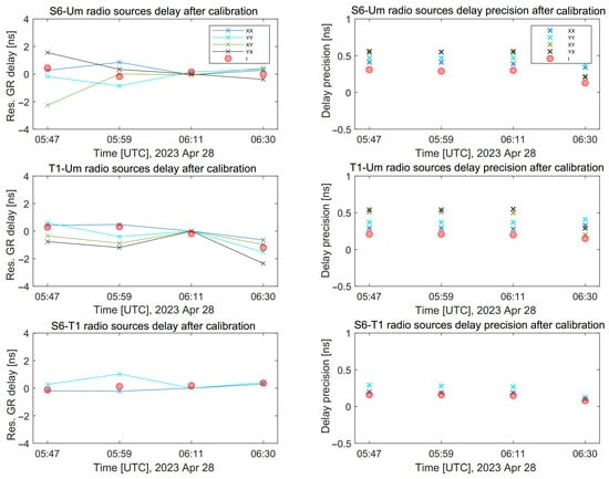
Figure 9.
Fringe-fitting residual group delays and delay precision for the single-scan integration of radio source.
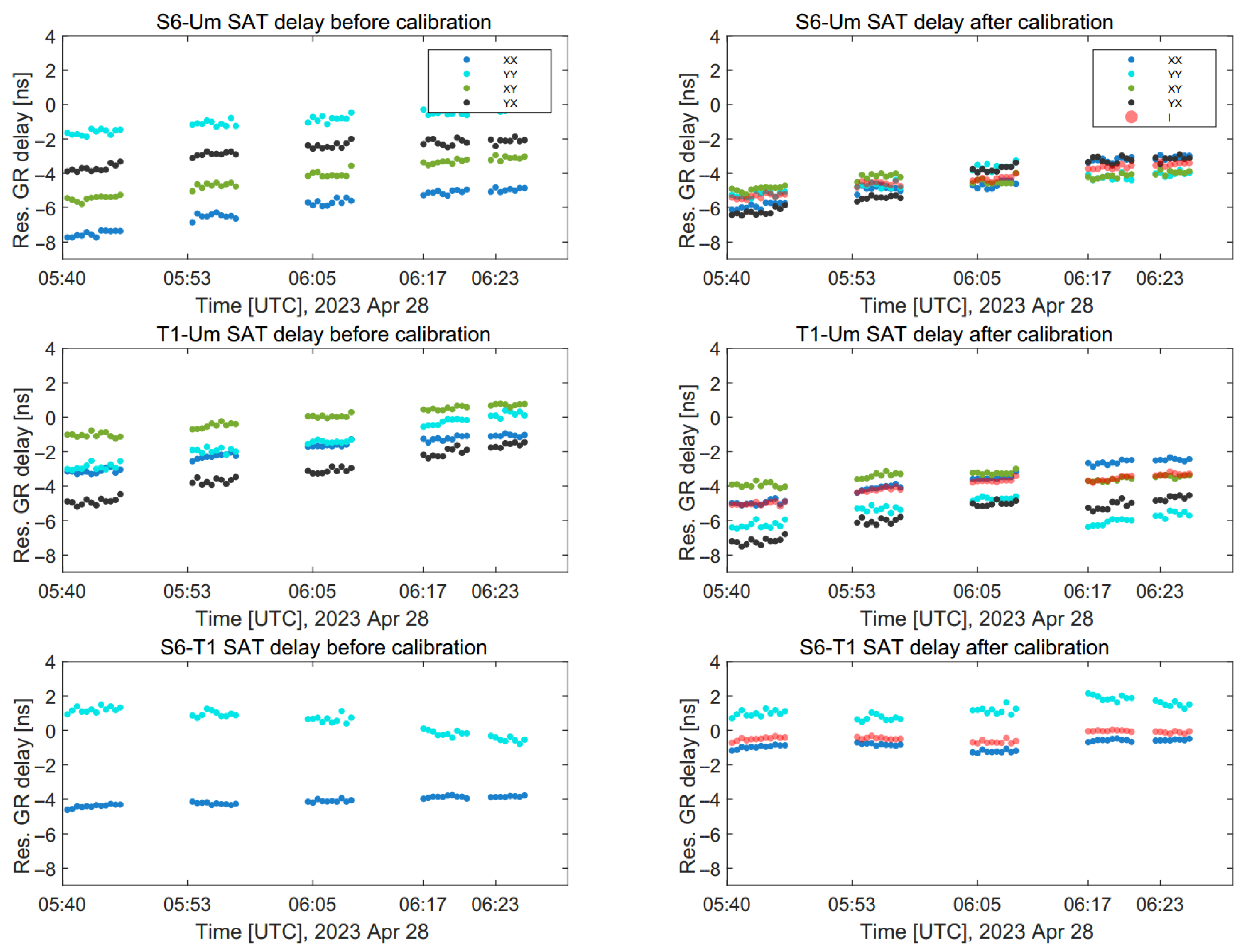
We employed a fringe fitting integration of 30 s for the satellite because its signals are much stronger than a radio source. The first fringe fitting process was conducted on all polarization products, followed by a second fringe fitting XX/YY/XY/YX and I (see Section 3.3.2 and Figure 5). The obtained residual delays are shown in Figure 10. The left column shows the residual delays when the three baselines were not calibrated. The right column shows the residual delays after calibration, with a median residual delay of the I (red) for S6-Um of −3.87 ns, T1-Um of -3.73 ns, and S6-T1 of −0.43 ns.
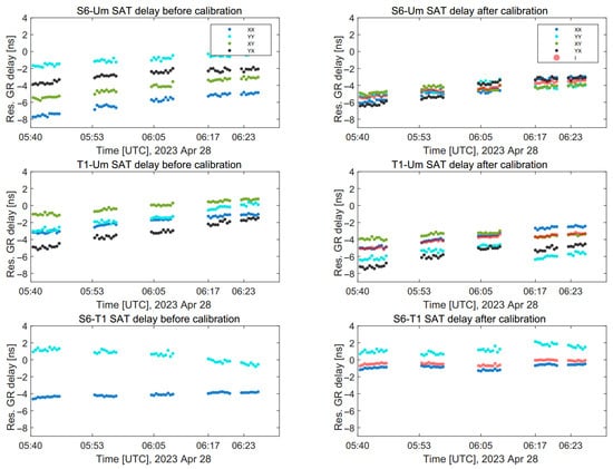
Figure 10.
Comparison of fringe fitting residual group delays between satellite scans uncalibrated and calibrated using the reference scan. Delays plotted versus time are indicated as minutes since 2023y118d05h40m00s.
In contrast, the residual group delays (Figure 10, right column) after delay/phase calibration and polarization combination exhibit smaller differences between the polarization products and shows a systematic variation with time. Some residual delays still occur between XX/YY/XY/YX, similar to the first scan of the T1-Um and S6-T1 baselines (Figure 10, right column). Essentially, we attribute the delay issues to three effects: (1) the SNR of certain polarization products of satellite signals is too weak to be calibrated correctly; (2) the ionospheric and atmospheric delays are not completely corrected; and (3) the short baseline distance of S6-T1 which results in radio-frequency interference (RFI).
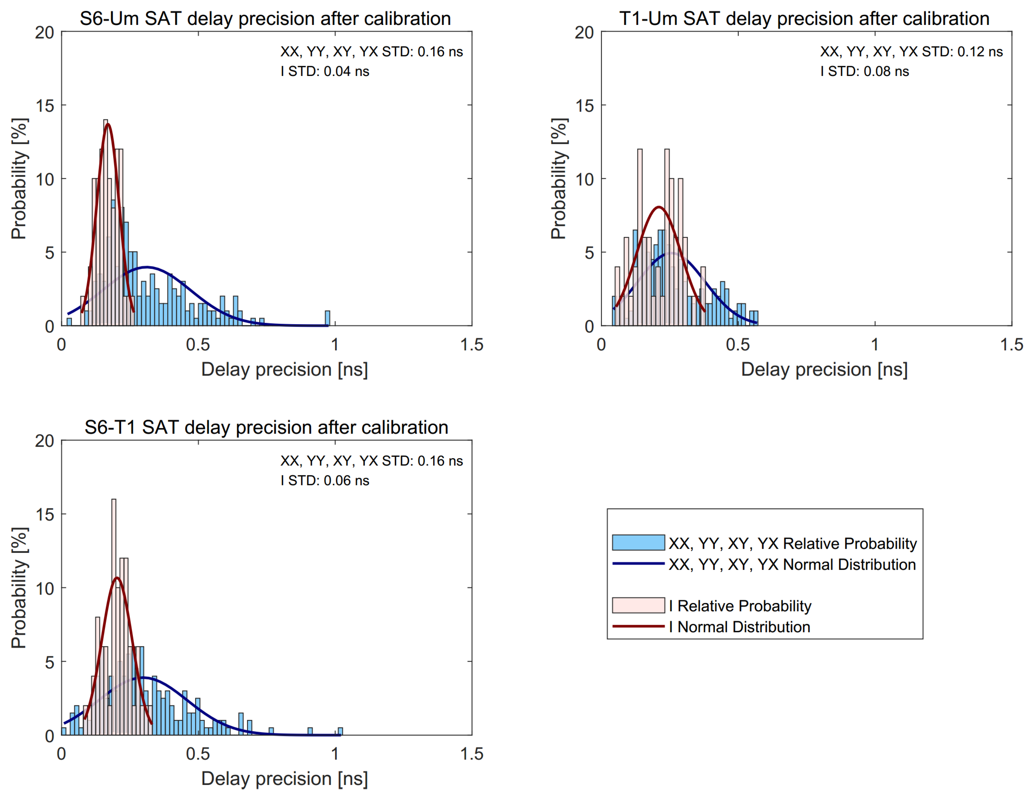
Figure 11 shows a comparison of the delay precision of the three baselines following the second fringe fitting of the satellite. The blue color indicates the relative probability distribution of the delay precision across the total XX/YY/XY/YX. In contrast, the pink color illustrates the delay precision of I. The delay and delay precision statistics after the second fringe fitting of the satellite scans are presented in Table 4. The scan results show good agreement between the XX/YY/XY/YX and I in terms of the delay precision. The delay precision values are typically 0.01–1.02 ns and the standard deviations are in the 0.12–0.16 ns range for XX/YY/XY/YX. Conversely, these values are 0.05–0.38 ns and 0.04–0.08 ns, respectively, for I. The smaller values of I demonstrate an improvement in delay precision. Evidently, the delay precision of S6-Um after the polarization combination is relatively better, with a median value of 0.16 ns. The delay precision values of the satellite and radio source are at the level of 0.1 ns, confirming that the results are reliable.
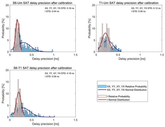
Figure 11.
Relative probability distribution of the delay precision in satellite signals, corresponding to the S6-Um, T1-Um, and S6-T1 baselines.
Table 4.
Residual delays and delay precision of SAT-C5GD on different baselines after calibration.
The dominant effect of polarization combination is expected to be imperfect calibration of the four polarization products. In the T1-Um baseline example, the residual delays after calibration (Figure 10, right column) are most prominent among the XX, YY, XY, and YX products. In contrast, the delay precision values distribution of I (Figure 11, pink) are more discrete compared with the S6-Um and S6-T1 baselines, exhibiting lower delay precision and poorer polarization combinations. As implied by Figure 11, some delay precision values of XX/YY/XY/YX are smaller than those for I, especially for the S6-T1 baseline, primarily owing to larger residual delays among the XX/YY/XY/YX products. This results in a degradation of the polarizations combination of some scans. We attributed this issue to be the same as that for the residual delay in the T1-Um baseline highlighted above.
4.2. Discussion
We consider the first observation results of the SAT-C5GD satellite encouraging. The experimental residual delays are at a similar level of a few nanoseconds, as reported in the study by McCallum et al. [19], who conducted an experiment to observe GNSS signals using the Australian VGOS array. Sun et al. [11] conducted experiments on the APOD satellite with the AuScope array. Sun et al. processed only the satellite signals in circular polarization without calibration using radio sources and yielded delay precision at the level of 0.1 ns.
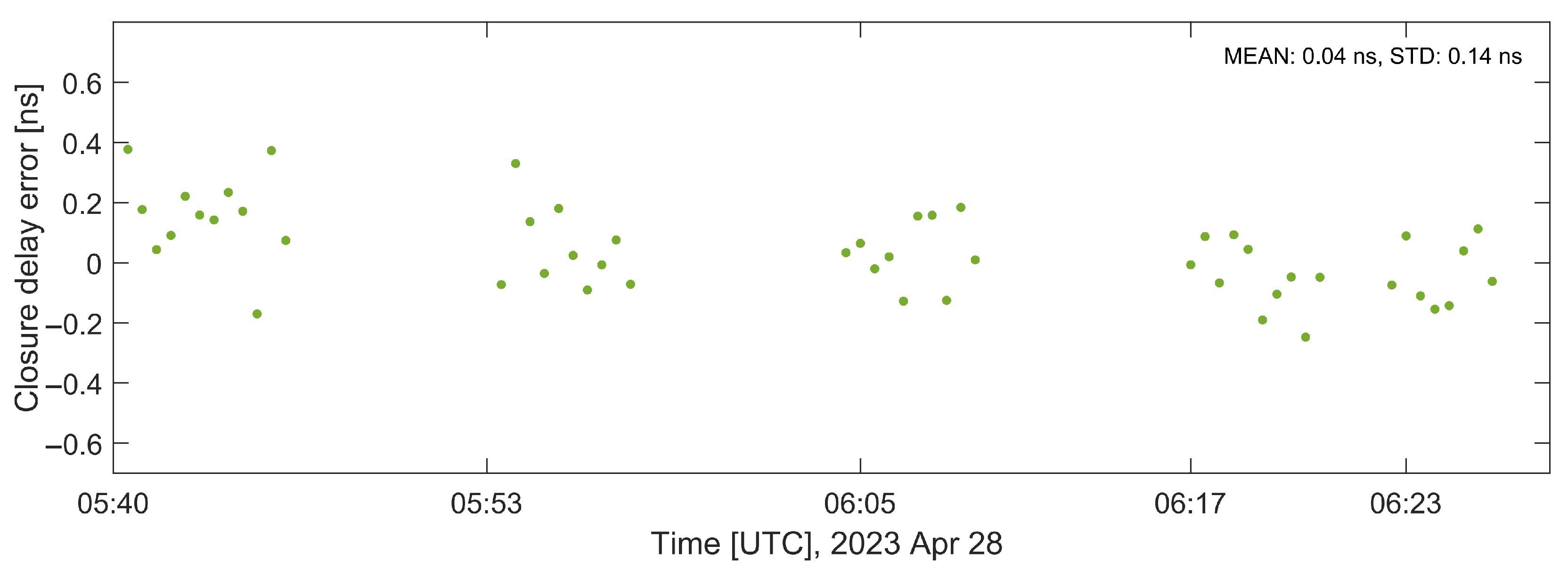
We investigated the closure delay on the three baselines. The closure delay is defined as follows:
In theory, the closure delay should be equal to zero if the delay values of , , and are substituted into Equation (7). However, owing to errors introduced during the delay measurement process, the actual closure delay is not zero. The closure-delay standard deviation (STD) is an indicator of the delay precision.
The closure delay on the three baselines was obtained from the residual delays (Figure 10, right column) of the SAT-C5GD scans. As shown in Figure 12, examining the closure delay of SAT-C5GD shows a variation in the range of −0.2 to 0.2 ns, with a mean of 0.04 ns and a STD of 0.14 ns. The delay precision is at the same level as the closure delay STD. As such, we conclude that no significant systematic errors exist in the delay measurement, primarily owing to the calibration strategy used.
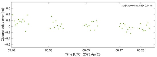
Figure 12.
Closure delay error on the three baselines.
The comparative analysis of the SAT-C5GD closure delay obtained by Li et al. [26] and that of the present study is outlined in Table 5. The co-located stations are URUMQI 26-m (Ur) and URUMQI 13-m (Um), and TIANMA 65-m (Tm) and TIANMA 13-m (T1). BEIJING 50-m, Ur, and Tm have a long baseline; however, the SESHAN 13-m (S6) and T1 baseline is significantly shorter. “Freq.” in the table provides the channel bandwidth and number of channels. This study utilized DOR tones in a single channel with a fixed bandwidth of 32 MHz for the VGOS. Our experimental results demonstrate a measured precision of 0.14 ns, which is 2.8 times that of the study by Li et al. Evidently, the smaller delay precision values are preferable. Although the present study demonstrated a lower level of delay precision than that obtained in the study by Li et al., the theoretical requirements have nonetheless been met. This limitation is primarily attributable to the smaller diameter of the antennas and inaccurate ionospheric and atmospheric correction.
Table 5.
Comparison of the SAT-C5GD results.
The precision obtained in this study may be sufficient for lunar exploration missions; however, it cannot cater to the exploitation of space-tie satellites for TRF improvement. The narrow bandwidth of DOR beacons is a challenge to improving the delay precision. In the future, employing ultra-wideband beacons in space-tie low and medium Earth orbit (LEO/MEO) satellites for combined-orbit determination would be helpful to achieve a delay precision better than 10 ps.
5. Conclusions and Outlook
We developed a unique data processing pipeline suitable for VGOS data in the dual linear polarization mode applied to the differential observation of satellites. An observation experiment of the Chang’e 5 lunar orbiter was conducted using the three VGOS antennas in China. The results show the residual delays at the level of a few nanoseconds, with a median delay precision of 0.16 ns in the 30 s integration of a single channel. The data analysis reveals that the standard deviation of the baseline closure delay is 0.14 ns. These results demonstrate that the data processing system is reliable and efficient and that VGOS observation of artificial satellites is feasible.
In future studies, we will optimize the observation schedule, conduct additional observation experiments, and upgrade the data processing system for VGOS satellite observation. The data processing upgrade will include delay and phase calibration spanning multiple channels, polarization combination, and ionosphere and atmospheric correction.
We would like to stress that there is yet more development necessary to make VGOS observations of satellites sufficiently precise and accurate. This study lays the groundwork for these developments. We believe the study findings will contribute to the application of VGOS in space-tie satellite missions utilizing geodetic techniques.
Author Contributions
Conceptualization, J.G. and F.S.; project administration, F.S.; VLBI schedule, F.T. and Y.S.; software, J.G.; data processing, J.G., X.H. and Y.H.; writing—original draft, J.G.; writing—review and editing, J.G., F.S. and X.H. All authors have read and agreed to the published version of the manuscript.
Funding
This work was supported by the Astrometric Reference Frame project, Grant No. JZZX-0102. And supported by the National Natural Science Foundation of China, Grant No. 12303098.
Data Availability Statement
The data presented in this study are openly available at https://pan.cstcloud.cn/s/iMeKCaRT5s (accessed on 3 July 2025).
Acknowledgments
This study made use of three VGOS stations. The data processing has been carried out on the Shanghai VLBI Correlator, hosted and operated by the Shanghai Astronomical Observatory at the Chinese Academy of Sciences. We acknowledge Cong Liu’s support in VGOS observations and Zhong Chen’s contribution in managing data transmission from Urumqi.
Conflicts of Interest
The authors declare no conflict of interest. The founding sponsors had no role in the design of the study; in the collection, analyses, or interpretation of data; in the writing of the manuscript; or in the decision to publish the results.
References
- Niell, A.; Barrett, J.; Burns, A.; Cappallo, R.; Corey, B.; Derome, M.; Eckert, C.; Elosegui, P.; McWhirter, R.; Poirier, M.; et al. Demonstration of a Broadband Very Long Baseline Interferometer System: A New Instrument for High-Precision Space Geodesy. Radio Sci. 2018, 53, 1269–1291. [Google Scholar] [CrossRef]
- Schüler, T.; Kronschnabl, G.; Plötz, C.; Neidhardt, A.; Bertarini, A.; Bernhart, S.; La Porta, L.; Halsig, S.; Nothnagel, A. Initial Results Obtained with the First TWIN VLBI Radio Telescope at the Geodetic Observatory Wettzell. Sensors 2015, 15, 18767–18800. [Google Scholar] [CrossRef]
- Altamimi, Z.; Rebischung, P.; Collilieux, X.; Métivier, L.; Chanard, K. ITRF2020: An augmented reference frame refining the modeling of nonlinear station motions. J. Geod. 2023, 97, 47. [Google Scholar] [CrossRef]
- Zoulida, M.; Pollet, A.; Coulot, D.; Perosanz, F.; Loyer, S.; Biancale, R.; Rebischung, P. Multi-technique combination of space geodesy observations: Impact of the Jason-2 satellite on the GPS satellite orbits estimation. Adv. Space Res. 2016, 58, 1376–1389. [Google Scholar] [CrossRef]
- Männel, B. Co-Location of Geodetic Observation Techniques in Space. Ph.D. Thesis, ETH Zürich, Zürich, Switzerland, 2016. [Google Scholar]
- Delva, P.; Altamimi, Z.; Blazquez, A.; Blossfeld, M.; Böhm, J.; Bonnefond, P.; Boy, J.P.; Bruinsma, S.; Bury, G.; Chatzinikos, M.; et al. GENESIS: Co-location of geodetic techniques in space. Earth Planets Space 2023, 75, 5. [Google Scholar] [CrossRef]
- Plank, L. VLBI Satellite Tracking for the Realization of Frame Ties. Ph.D. Thesis, Vienna University of Technology, Vienna, Austria, 2014. [Google Scholar]
- Anderson, J.M.; Beyerle, G.; Glaser, S.; Liu, L.; Männel, B.; Nilsson, T.; Heinkelmann, R.; Schuh, H. Simulations of VLBI observations of a geodetic satellite providing co-location in space. J. Geod. 2018, 92, 1023–1046. [Google Scholar] [CrossRef]
- Klopotek, G.; Hobiger, T.; Haas, R.; Otsubo, T. Geodetic VLBI for precise orbit determination of Earth satellites: A simulation study. J. Geod. 2020, 94, 56. [Google Scholar] [CrossRef]
- Schunck, D.; McCallum, L.; Calves, G.M. Simulating VLBI observations to BeiDou and Galileo satellites in L-band for frame ties. J. Geod. Sci. 2024, 14, 20220168. [Google Scholar] [CrossRef]
- Sun, J.; Tang, G.S.; Shu, F.C.; Li, X.; Liu, S.; Cao, J.; Hellerschmied, A.; Böhm, J.; McCallum, L.; McCallum, J.; et al. VLBI observations to the APOD satellite. Adv. Space Res. 2018, 61, 823–829. [Google Scholar] [CrossRef]
- Hellerschmied, A.; McCallum, L.; McCallum, J.; Sun, J.; Böhm, J.; Cao, J. Observing APOD with the AuScope VLBI Array. Sensors 2018, 18, 1587. [Google Scholar] [CrossRef]
- Plank, L.; Hellerschmied, A.; McCallum, J.; Böhm, J.; Lovell, J. VLBI observations of GNSS-satellites: From scheduling to analysis. J. Geod. 2017, 91, 867–880. [Google Scholar] [CrossRef]
- Schunck, D.; McCallum, L.; Calves, G.M. On the Integration of VLBI Observations to GENESIS into Global VGOS Operations. Remote Sens. 2024, 16, 3234. [Google Scholar] [CrossRef]
- Shu, F.C.; Petrov, L.; Jiang, W.; Xia, B.; Jiang, T.; Cui, Y.; Takefuji, K.; McCallum, J.; Lovell, J.; Yi, S.O.; et al. VLBI Ecliptic Plane Survey: VEPS-1. Astrophys. J. Suppl. Ser. 2017, 230, 13. [Google Scholar] [CrossRef]
- Li, P.J.; Fan, M.; Huang, Y.; Hu, X.; Chang, S.; Shan, Q. Real-time orbit determination for transfer orbit and lunar orbit of the CE-5T1 probe. Sci. Sin. Phys. Mech. Astron. 2017, 47, 125903. [Google Scholar] [CrossRef]
- Liu, Q.; Huang, Y.; Shu, F.C.; Wang, G.; Zhang, J.; Chen, Z.; Li, P.; Ma, M.; Hong, X. VLBI technique for the orbit determination of Tianwen-1. Sci. Sin. Phys. Mech. Astron. 2022, 52, 239507. [Google Scholar] [CrossRef]
- Nothnagel, A.; Artz, T.; Behrend, D.; Malkin, Z. International VLBI Service for Geodesy and Astrometry: Delivering high-quality products and embarking on observations of the next generation. J. Geod. 2017, 91, 711–721. [Google Scholar] [CrossRef]
- McCallum, L.; Schunck, D.; McCallum, J.; McCarthy, T. An experiment to observe GNSS signals with the Australian VGOS array. Publ. Astron. Soc. Pac. 2025, 137, 045002. [Google Scholar] [CrossRef]
- Park, R.; Folkner, W.M.; Jones, D.L.; Border, J.S.; Konopliv, A.S.; Martin-Mur, T.J.; Dhawan, V.; Fomalont, E.; Romney, J.D. Very Long Baseline Array Astrometric Observations of Mars Orbiters. Astron. J. 2015, 150, 121. [Google Scholar] [CrossRef]
- Deller, A.T.; Brisken, W.F.; Phillips, C.J.; Morgan, J.; Alef, W.; Cappallo, R.; Middelberg, E.; Romney, J.; Rottmann, H.; Tingay, S.J. DiFX-2: A More Flexible, Efficient, Robust, and Powerful Software Correlator. Publ. Astron. Soc. Pac. 2011, 123, 275. [Google Scholar] [CrossRef]
- CCSDS. Recommendations for Space Data System Standards: Radio Frequency and Modulation Systems, Part 1, Earth Stations and Spacecraft, Recommended Standard 401.0-B; Consultative Committee for Space Data Systems, CCSDS Secretariat, NASA: Washington, DC, USA, 2009. [Google Scholar]
- Gan, J.Y.; Guo, S.G.; He, X.; Liu, C.; Sun, Z.; Li, J.; Ma, L.; Shu, F.; Zhang, X. Research of VGOS baseband data pre-processing system. Chin. Space Sci. Technol. 2022, 42, 46–53. [Google Scholar] [CrossRef]
- Cappallo, R. Delay and Phase Calibration in VGOS Post-Processing. In Proceedings of the International VLBI Service for Geodesy and Astrometry 2016 General Meeting, Johannesburg, South Africa, 13–17 March 2016; NASA/CP-2016-219016. pp. 61–64. [Google Scholar]
- CCSDS. Delta-DOR—Technical Characteristics and Performance, Report Concerning Space Data System Standards, Green Book, 500.1-G-2; Consultative Committee for Space Data Systems, CCSDS Secretariat, NASA: Washington, DC, USA, 2019. [Google Scholar]
- Li, T.; Liu, L.; Zheng, W.M.; Zhang, J. The Precision Analysis of the Chinese VLBI Network in Probe Delay Measurement. Res. Astron. Astrophys. 2022, 22, 035001. [Google Scholar] [CrossRef]
Disclaimer/Publisher’s Note: The statements, opinions and data contained in all publications are solely those of the individual author(s) and contributor(s) and not of MDPI and/or the editor(s). MDPI and/or the editor(s) disclaim responsibility for any injury to people or property resulting from any ideas, methods, instructions or products referred to in the content. |
© 2025 by the authors. Licensee MDPI, Basel, Switzerland. This article is an open access article distributed under the terms and conditions of the Creative Commons Attribution (CC BY) license (https://creativecommons.org/licenses/by/4.0/).