Abstract
Surface ozone (O3) is a multifaceted threat that not only deteriorates the environment but also poses risks to human health. Here, we estimated the seamless hourly surface O3 in China using Extreme Gradient Boosting (XGBoost) with multisource data fusion to investigate spatiotemporal differences in O3 during multistage COVID-19, and the response of O3 variation to meteorology and emissions were explored using Shapley Additive Explanations (SHAP) and WRF-Chem. The results indicate that the optimized model demonstrated higher accuracy, with CV-R2 of 0.96–0.97 and RMSE of 4.58–5.00 μg/m3. Benefitting from the full coverage of the dataset, the underestimated O3 was corrected and hotspots of short-term O3 pollution events were successfully captured. O3 increased by 16.8% during the lockdown, with high values clustered in the north and west, attributed to the weakened urban NOx titration resulting from reduced emissions. During the control and regulation period, O3 levels declined year by year. O3 exhibited significant fluctuations in the Pearl River Delta but remained stable in western China, with both regions demonstrating high sensitivity to meteorological variability. Among these, solar radiation and temperature were the key meteorological factors. The seamless high-resolution O3 datasets will enable more insightful analyses regarding the spatiotemporal characterization and cause analysis.
1. Introduction
Ozone (O3) is a potent oxidant that interacts with solar shortwave and outgoing longwave radiation, which can affect climate change [1]. While approximately 90% of O3 exists in the upper atmosphere or stratosphere, surface O3 poses significant risks to human health [2], including an increased incidence of respiratory and cardiovascular conditions [3,4]. Since 2013, China has implemented a series of air pollution control measures that have significantly reduced sulfur dioxide (SO2), nitrogen oxides (NOx), and particulate matter. However, surface O3 has increased by 20% [5,6]. The daily maximum 8-h average (MDA8) O3 concentration in urban areas of China during the warm season is accelerating at an alarming rate of 2.4 ppb yr−1 (5%), surpassing the rate of increase in other regions worldwide [7].
The outbreak of the COVID-19 pandemic caused unprecedented social impacts worldwide and led to reductions in air pollutant levels across most regions [8,9,10,11,12]. In order to limit the spread of the virus, China implemented lockdown measures that significantly decreased anthropogenic emissions [13]. During this period, SO2, NO2, CO, and PM2.5 in China decreased by 17.6%, 15.8%, 11.1% and 3.0%, respectively. However, the concentration of surface O3 increased by 11.4%. The COVID-19 pandemic served as a “natural experiment” occurring during a period of rising O3 levels, offering a unique opportunity to evaluate O3 variations and response to emission controls. While several studies have only reported the sharp rise in surface O3 during the early stage of the pandemic, research on O3 variations and response mechanisms across the multiple stages of the pandemic remains limited. As a secondary pollutant, O3 forms through photochemical reactions involving nitrogen oxides (NOx = NO + NO2) and volatile organic compounds (VOCs) [14,15]. In addition to photochemical reactions, meteorological conditions also alter O3 levels through various physical and chemical processes [16]. Consequently, the combined effects of complex chemical buffering and varying meteorological conditions may amplify O3 pollution in certain regions [17,18]. During the multistage COVID-19 pandemic, changing emission patterns and meteorological conditions continuously influenced O3 [19]. A comprehensive understanding of O3 variations and response mechanisms during the COVID-19 pandemic can provide a basis for developing effective strategies to mitigate surface O3 pollution.
Accurate and reliable monitoring data are essential for tackling the persistent surface O3 pollution. Ground-based observations are the primary method for studying O3, offering high precision and strong temporal continuity. However, due to the uneven distribution of monitoring stations, remote areas, deserts, and mountainous regions lack sufficient monitoring sites, making them unable to meet the requirements for continuous spatial monitoring [20,21]. To supplement limited ground-based data, satellite remote sensing has emerged as a pivotal tool for O3 pollution studies, leveraging backscattered radiation from Earth’s atmosphere and surface [22]. Although satellite monitoring provides extensive O3 distribution, ultraviolet measurements exhibit limited sensitivity to surface O3, which typically comprises only a minor fraction (a few percent) of the total column [23]. On the other hand, cloud contamination frequently degrades the accuracy of satellite retrievals [24]. These inherent limitations result in notable differences between ground-based and satellite-derived O3 levels and distribution. Constructing high-resolution, spatiotemporally continuous surface O3 data remains a major challenge.
To overcome the limitations of single-source observations, previous studies have aimed to establish the connection between satellite column concentrations and surface O3 through statistical models, such as geographically weighted regression [25] and generalized additive models [26]. Recently, machine learning (ML) has demonstrated key advantages in dealing with complex nonlinear problems. It not only addresses high-dimensional uncertainties but also improves the training effect as sample size increases [27]. Numerous studies have confirmed that algorithms such as decision trees [28], support vector machines [29], random forests [30], and neural networks [31] precisely model the nonlinear relationships between input features and predictions. Among these, the Extreme Gradient Boosting (XGBoost) ensemble algorithm has shown outstanding performance in modeling complex nonlinear relationships among multiple feature variables, exhibiting excellent fitting ability and high training efficiency [32,33]. Numerous studies have demonstrated the predictive capability of existing approaches at daily timescales, but accurate hourly scale O3 estimation remains insufficiently explored. Moreover, 24-h data are of utmost importance for determining MDA8, analyzing fine spatiotemporal O3 variations, and the mechanisms of O3 pollution events.
In this study, we employed XGBoost algorithm to integrate atmospheric composition retrieved from high-resolution satellites, high-temporal reanalysis meteorological data, high-precision ground observation station data, and multisource geographic elements to establish seamless hourly surface O3 dataset in China during the multistage COVID-19 pandemic from 2019 to 2022. Unlike traditional statistical methods that mostly rely on individual observation data points, our model extends the impact of satellite and meteorological data on O3 to an hourly scale by performing randomized search each day for hyperparameter tuning, effectively filling in the missing data and enhancing the accuracy of O3 estimation. Seamless high-resolution O3 mapping aims to evaluate the spatiotemporal differences in O3 during the multistage COVID-19 pandemic. Compared to most previous studies that primarily focused on the early phase, this study achieved more comprehensive coverage in both space and time. In addition, the Weather Research and Forecasting-Chemistry (WRF-Chem) model and Shapley Additive Explanations (SHAP) were independently used to quantify the contributions of meteorology and emissions to O3 formation, offering theoretical support for O3 pollution control.
2. Materials and Methods
2.1. Study Period
This study is categorized into three periods to analyze the impacts of various emission reduction scenarios on O3 levels (Table 1). The first period, from 20 January to 17 February 2020, was identified as the lockdown period (LP), during which China implemented strict lockdown measures, resulting in predominant reductions in anthropogenic emissions. The same period in 2021 was designated as the control period (CP), characterized by relaxed epidemic prevention measures, with a focus on mitigating the rebound of air pollution amid the gradual resumption of economic activities. The corresponding period in 2022 was designated as the regulation period (RP), during which regional control intensity was dynamically adjusted based on the level of COVID-19 risk. A one-month period starting on 20 January was selected as the research timeframe, as it marked the nationwide spread of COVID-19 and the official implementation of national control policies.

Table 1.
COVID-19 period name definition.
2.2. Data Sources
2.2.1. Ground-Based Observations
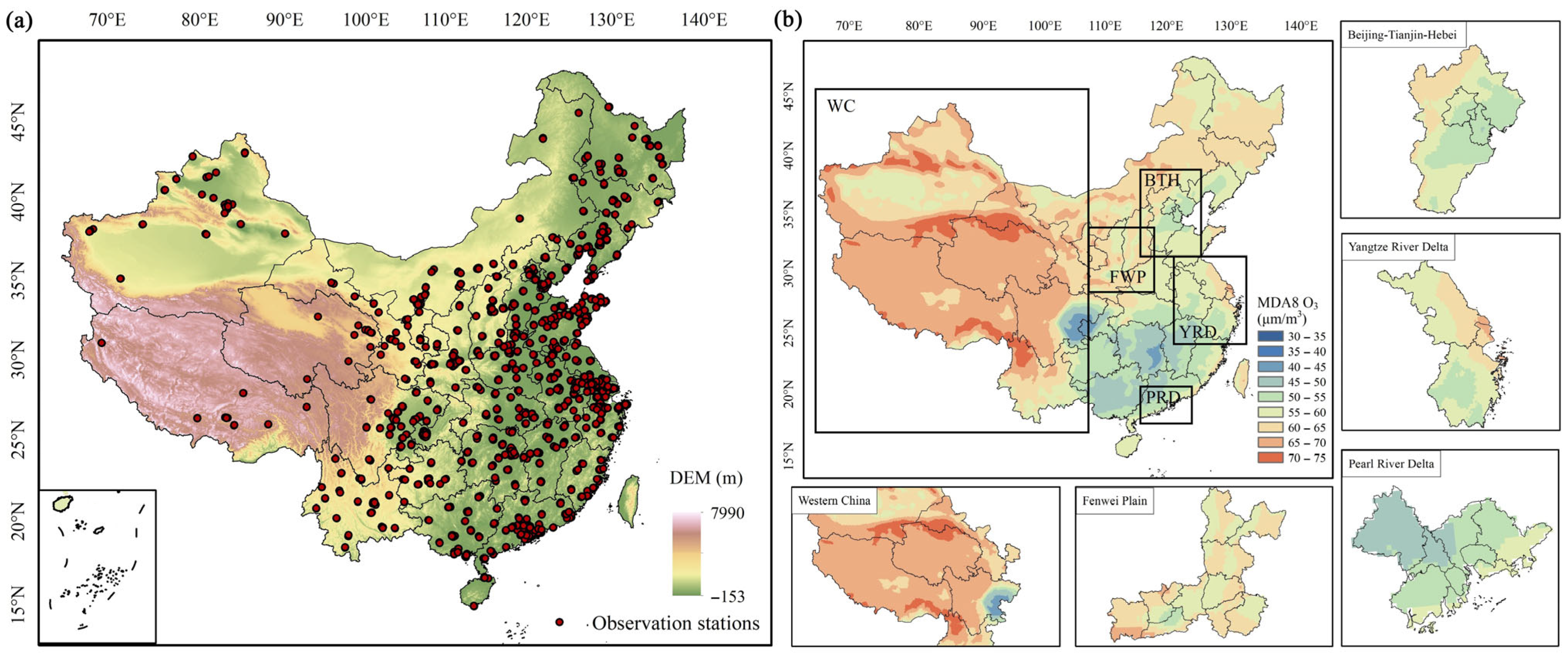
Surface air pollutant data were available from hourly observations provided by the China National Environmental Monitoring Center (CNEMC). National air quality monitoring commenced in 2013 and expanded to cover 337 prefecture-level cities by 2020. This study used the hourly O3 and NO2 from 1619 air quality monitoring stations across various regions of China, with sampling conducted from 2020 to 2022 (Figure 1a). Following the method proposed by Wang et al. [34], we treated observations with values exceeding the upper threshold or negative values as invalid, and excluded data points greater than 700 μg/m3 and less than 0 μg/m3. Second, observations with deviations (observations minus monthly mean value) greater than 100 μg/m3 were also removed. We focused on the spatial distribution of O3 across the entire territory of China and in typical regions, including the Beijing-Tianjin-Hebei (BTH), Yangtze River Delta (YRD), Pearl River Delta (PRD), Fenwei Plain (FWP), and western China (WC), as illustrated in Figure 1b.
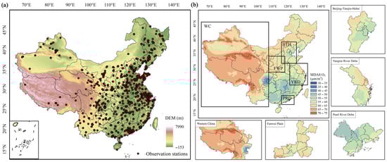
Figure 1.
(a) Spatial distribution of the observation stations on digital elevation model of China. (b) The spatial distribution of average surface O3 concentrations from 20 January to 17 February (2020–2022) were estimated based on XGBoost model. The black boxes highlight the BTH, YRD, PRD, FWP, and WC.
2.2.2. Remote Sensing Measurements
The hyperspectral TROPOspheric Monitoring Instrument (TROPOMI), launched by the European Space Agency (ESA) on 13 October 2017, is the only payload on the Sentinel-5P satellite. The initial imaging resolution was 7 km × 3.5 km [35], but has since been upgraded to the higher resolution of 5.5 km × 3.5 km [36]. TROPOMI features a high signal-to-noise ratio and includes four independent spectrometers, enabling more accurate retrieval of O3 column concentration at various altitudes in the atmosphere [37,38]. However, extensive cloud cover during winter in high-latitude regions may lead to data gaps in TROPOMI. To address this limitation, we incorporate the OMI-retrieved data as input variables into the ML framework. The two sensors operate on sun-synchronous orbits and have similar local overpass times (approximately 13:30–13:45 local time). ML is a black-box approach capable of integrating information from multiple satellite instruments to improve the spatial representation of O3 and enable more robust estimations in regions where TROPOMI observations are missing [39,40]. The study used O3, nitrogen dioxide (NO2), and formaldehyde (HCHO) column concentrations. To ensure data accuracy, a stringent screening threshold was applied. The extraction boundary of the study area was expanded by 0.3°. The outliers with qa_value < 0.75, zenith_angle < 70° and cloud_fraction_crb > 0.3 were removed, and adjacent swaths were merged [40].
Surface O3 is produced through nonlinear chemical processes involving reactions of NOx and VOCs. Here, NO2 is a crucial component of NOx, while HCHO appears as a high-yield intermediate in the photochemical oxidation of VOCs. Therefore, HCHO and NO2 are essentially considered the tracers of VOCs and NOx [41]. Owing to this, the ratio of satellite-derived column concentrations of HCHO to NO2 (FNR) can be exploited to identify the formation mechanism of surface O3 [42,43]. When FNR < 1 represents VOCs-sensitive, conversely, FNR > 2 depicts NOx-sensitive [44]. The FNR value existing between 1 and 2 indicates a transitional state where both VOCs and NOx influence O3 production [45].
2.2.3. Meteorological and Auxiliary Data
The hourly reanalysis meteorological dataset, comprising 16 O3-related parameters, was obtained from the European Centre for Medium-Range Weather Forecasts Reanalysis, Version 5 (ERA5). We also gathered auxiliary data with potential impacts on O3 formation. The elevation data were gathered from the ASTER Global Digital Elevation Model (AGDEM) with a spatial resolution of 30 m. Vegetation and land use influence the air quality; dense vegetation cover typically helps to mitigate pollution, whereas paved surfaces can contribute to warmer temperatures and boost production of secondary pollutants [46]. Land Use and Land Cover Change data (LUCC) were derived from Moderate-resolution Imaging Spectroradiometer (MODIS) satellites, categorizing 17 land types including urban areas, forests, and farmland. The Normalized Difference Vegetation Index (NDVI) was represented by the 1 km MOD13A3 product, which dynamically reflected vegetation distribution and changes across China. Additionally, emissions and economic activities can also influence the pollutant concentrations. The emissions inventory was obtained from the Multiresolution Emission Inventory of China (MEIC). Cloud-free nighttime light data were acquired from the Visible and Infrared Imaging Suite (VIIRS) onboard the Joint Polar-Orbiting Satellite System (JPSS) satellites. Population distribution data developed by the Oak Ridge National Laboratory (ORNL) were also incorporated. Table 2 illustrates all features used for ML.
Table 2.
Summary of detailed data used in XGBoost model.
2.3. Machine Learning Estimates Surface O3
2.3.1. XGBoost Model
XGBoost is an ensemble learning algorithm that employs distributed gradient boosting decision trees. Each decision tree was trained on the residual of the preceding tree. New trees were introduced to minimize the loss function, thereby gradually reducing the error. Leaf node predictions and tree complexity were tuned to optimize model performance. The XGBoost model incorporates model complexity along with the traditional loss function to assess the model’s generalization capability and computational efficiency, as follows:
where is the number of trees, is a function in the functional space, and is the complexity of the tree . During each iteration, the optimal is obtained by minimizing . A regularization term is included to prevent overfitting:
We calculated the score of each leaf node and determined the optimal tree structure. The score accounted for both impurity measures in the decision tree and the model complexity:
2.3.2. Model Development and Validation
The XGBoost model was constructed to estimate surface O3. Ground-based hourly O3 observations were used as the target variable, whereas the remaining variables served as input variables. All data were resampled to the same spatial resolution of 0.1° × 0.1° grid using the bilinear interpolation approach [47]. By performing spatiotemporal matching, we addressed spatial mismatch among datasets at varying longitudes and latitudes.
To optimize model performance and eliminate redundant input, recursive feature elimination (RFE) was applied for variable selection (Figure S1). This process reduced redundancy from irrelevant features while preserving variables critical to prediction accuracy. Based on the results of feature screening, the dataset was randomly divided into 70% for model training and 30% for testing. Generally, meteorological variables are the most important, but the ranking of variable importance results is different under different conditions. To account for this variability while maintaining a sufficient sample size, we found that adjusting the model parameters on a daily basis could obtain the best estimate of hourly O3 on that day. Therefore, we implemented an intensive optimization process that synergistically adjusted multiple hyperparameters. A ten-fold cross-validation (10-CV) combined with randomized grid search was employed to construct a model with the optimal parameter combination each day. These adjusted parameters were used for training the XGBoost model. We did not use a unified model because coarse-resolution modeling approaches may incur information loss when predicting fine temporal resolution data, thereby limiting the accurate characterization of hourly O3 dynamics.
We divided the dataset into training and validation sets at a nine-to-one ratio for each training iteration. The mapping relationship was validated through the training set, whereas precision of the trained model was evaluated using the validation set [48]. Statistical metrics, including the coefficient of determination (R2), mean absolute error (MAE), mean squared error (MSE), and root mean square error (RMSE), are as defined by Equations (6)–(9). represents the samples. and denote as the model observed values and predicted values, respectively.
2.3.3. Interpretability Analysis of Model
The model decision-making mechanism was investigated using SHAP to ascertain global interpretability, quantifying the contribution of each feature to the target variable. SHAP characterizes the complex relationships between input features and model outputs by computing the positive or negative contributions of each feature, providing insights into the decision-making process of the tree structure model. The formula is as follows:
where represents an iteration over all possible subsets () of that exclude feature to calculate the prediction difference of feature after adding subset (); and represent the output of the model for different combinations of features when the feature is present and absent. According to the SHAP value, red indicates feature value has a positive impact on the target variable, whereas blue signifies a negative impact. The proximity of the SHAP value to zero reflects the feature contribution to the prediction: values closer to zero indicate a smaller contribution, while values further from zero denote a greater influence on the prediction target.
2.4. WRF-Chem Simulation
The WRF-Chem ver.3.9.1 is an air quality model developed by the National Oceanic and Atmospheric Administration Forecast System Laboratory, which couples the chemical transport module (Chem) with the meteorological model (WRF) to reflect the real atmospheric conditions [49]. The model is configured with domains covering China with 34 vertical layers up to 50 hPa. For initial boundary meteorological conditions, we utilized the Final Reanalysis Data (FNL) global reanalysis data provided by the National Center for Environmental Prediction (NCEP), which featured a temporal resolution of 6 h and a spatial resolution of 1° × 1°. The model physics configuration included the Lin microphysics scheme [50], the Rapid Radiative Transfer Model (RRTM) radiation scheme [51], the Goddard Shortwave Radiation scheme [52], the Noah Land-Surface scheme [53], the Mellor-Yamada-Janjic TKE planetary boundary layer parameterization [54], and the Xu-Randall cloud effect [55]. The gas-phase chemical scheme integrated the RADM2 chemical mechanism, and the MADE/SORGAM aerosol coupled scheme [56]. Biogenic emissions were estimated from the Model for Emissions of Gases and Aerosols from Nature (MEGAN) [57], including monoterpenes, isoprene, and soil nitrogen. The anthropogenic emissions were based on the Multiresolution Emission Inventory for China (MEIC) at a spatial resolution of 0.25° × 0.25° on a monthly basis [58]. Further details are summarized in Table S1.
Sensitivity simulations were designed to quantify the respective impacts of meteorological conditions and anthropogenic emissions on surface O3 (Table 3). Considering the uncertainty in the emission inventory, we set up the experiment by fixing emissions while changing the meteorological conditions. The meteorology and emissions were fixed in Base from 20 January to 17 February 2019, representing the situation before the epidemic. Similarly, meteorology and emissions for Base_LP, Base_CP, and Base_RP were static for 2020, 2021, and 2022, respectively. Differences between each experiment and the base reflected the combined effects of meteorology and emissions on O3 formation. By comparing time periods of equal length, the effects of short-term meteorological anomalies can be minimized, thereby reducing potential impacts related to the Spring Festival [59]. For the comparative experiments EXP_LP, EXP_CP, and EXP_RP, emissions were fixed to 2019 levels, whereas the meteorology was synchronized to the corresponding years. The difference between Base_LP and EXP_LP quantified the emission-driven changes in O3 during the LP. The same approach was applied to CP and RP. Additionally, the difference between each EXP and the base in the corresponding year represented the meteorological impacts on O3 variations.
Table 3.
Experimental configurations for WRF-Chem modeling system.
3. Results
3.1. Performance Analysis of Model
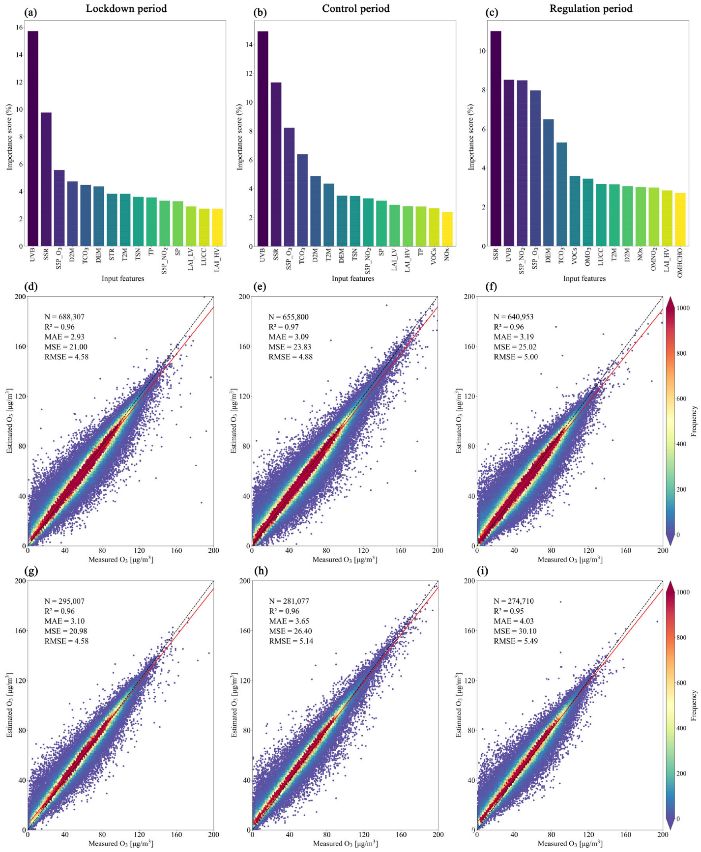
First, feature variables were selected using RFE. In each step of the RFE, an XGBoost model was built to rank input variables; the least important variable was removed and a new model base was created on this reduced set of input variables. We then determined the optimal set of features that significantly improved model performance. The variables finally used for model training and their importance rankings are shown in Figure 2a–c. The results revealed that downward UV radiation (UVB) and surface net solar radiation (SSR) were the most dominant variables for estimating surface O3, and scored from 0.08 to 0.12 and 0.08 to 0.16, respectively. Moreover, Satellite NO2 and O3 products play crucial roles in estimating surface O3, while total column ozone (TCO3), 2 m temperature (T2M), 2 m dewpoint temperature (D2M), and surface pressure (SP) also contribute to O3 formation. Unlike other periods, thermal radiation (STR) and snow layer temperature (TSN) exhibited higher importance scores during the LP period, accounting for 3.81% and 3.60%, respectively. In addition, VOCs and NOx were the key features in the CP and RP.
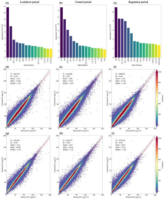
Figure 2.
XGBoost model importance ranking of top fifteen important variables in (a) LP, (b) CP, and (c) RP. (d–f) Represent scatter plots of 10-CV for the 70% dataset, resulting from hourly O3 estimates and O3 observations. (g–i) Represent scatter plots of blind test of 10-CV for the 30% dataset. Black dashed lines represent the 1:1 line, and red solid lines represent the best-fit lines derived from linear regression.
We first ensured a sufficient number of data samples in constructing the model. For each stage, the number of samples (N) exceeded 90,000, with more than 3000 valid samples. The only exception was 22 February 2020, with N = 2715 after outlier removal. In total, over 640,000 sample instances were included across ten-fold. To better present the results, the outcomes were summarized by period. The overall performance of the model was validated using sample-based 10-CV (Figure 2d–f). The results indicated that surface O3 estimates derived from the XGBoost model were highly consistent with O3 observations across China, and were generally concentrated near the 1:1 tangent line. The average CV-R2 values during the LP, CP, and RP were 0.96, 0.97, and 0.96, respectively. The mean MAE, MSE, and RMSE ranged from 2.93 to 3.19 μg/m3, 21.00 to 25.02 μg/m3, and 4.58 to 5.00 μg/m3, respectively. The high R2 and low error revealed that the model exhibited superior performance in estimating highly nonlinear hourly O3.
The model performance for the blind test was also evaluated (Figure 2g–i). The blind test results demonstrated high accuracy across the entire domain, with CV-R2 ranging from 0.95 to 0.96. The mean MAE, MSE, and RMSE ranged from 3.10–4.03 μg/m3, 20.98–30.10 μg/m3, and 4.58–5.49 μg/m3, respectively. These values were comparable to or slightly lower than those from the 10-CV on the 70% training dataset, indicating a strong generalization capability of the model. This superior efficacy can be attributed to an intensive optimization process, during which multiple hyperparameters were jointly tuned. This coordinated strategy significantly improved the overall accuracy of hourly O3 estimation. It is noteworthy that the statistical values across the three stages showed minimal differences, further indicating that the model is robust and reliable. Its performance was not affected by spatiotemporal heterogeneity, meeting the requirements for accurate hourly surface O3 estimation.
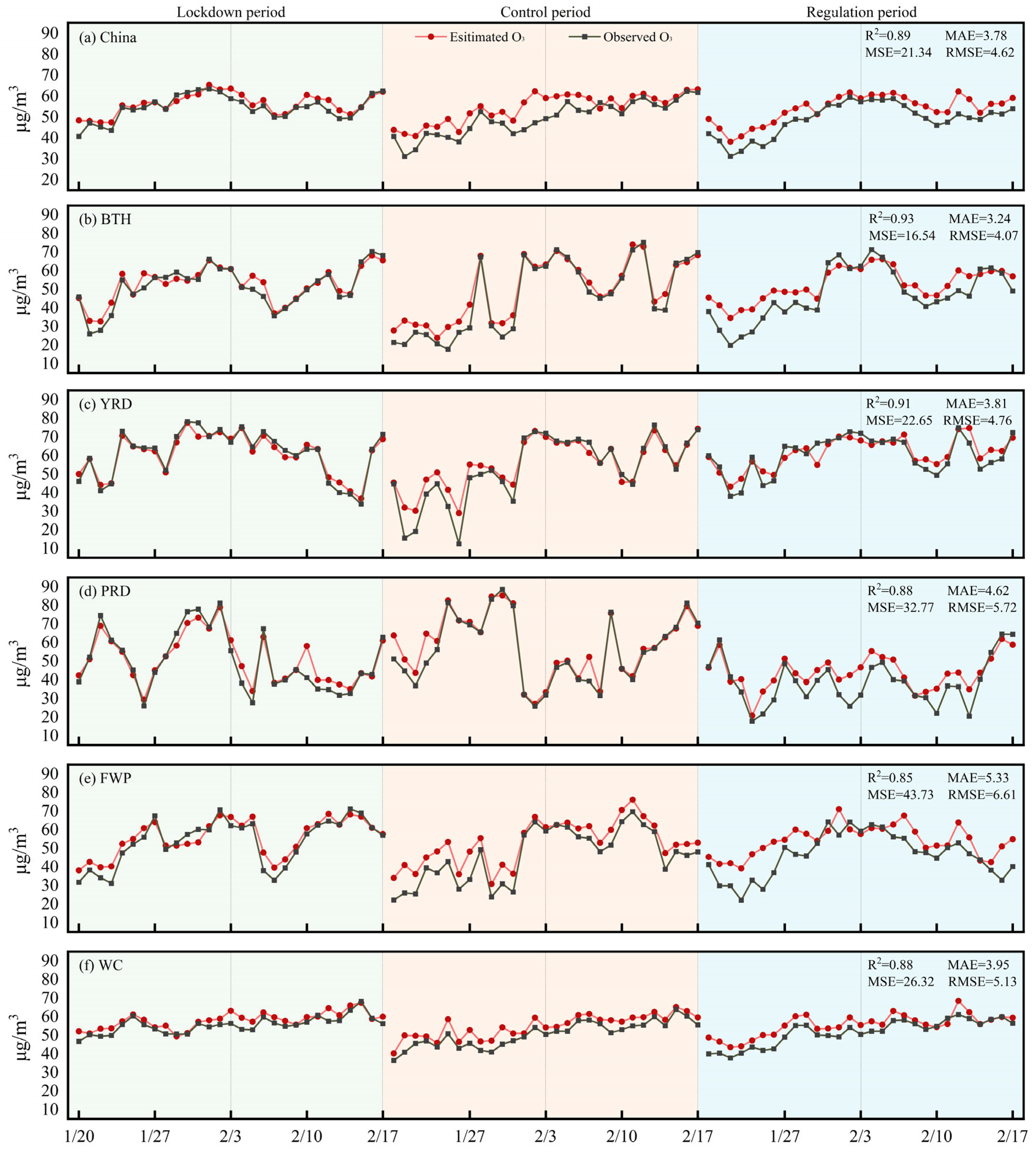
Figure 3 illustrates the temporal performance in China and typical regions. All O3 estimates were calculated using collocated ground monitoring data and validated against corresponding station observations. The results indicate that the O3 estimates in China show good agreement with observations, with an R2 of 0.89, MAE of 3.78 μg/m3, MSE of 21.34 μg/m3, and RMSE of 11.28 μg/m3. The differences between observed and estimated O3 are generally small. From a regional perspective, the model effectively captured O3 variations across five typical regions, demonstrating strong predictive powers (R2 = 0.85–0.93, RMSE = 4.07–6.61 μg/m3). The model performs best in regions with denser monitoring networks, such as the BTH and YRD, with most stations having high R2 above 0.9 and RMSE below 5 μg/m3. By contrast, the model performs relatively less consistently in the PRD, WC, and FWP, with R2 values of 0.88, 0.88, and 0.85, respectively. This may be attributed to greater uncertainties due to complex natural and meteorological influences [60]. The model estimates are highly consistent with observed temporal trends and effectively reproduce abnormal fluctuations in O3 levels, including sudden spikes or significant drops in the urban agglomeration (BTH, YRD and PRD). In relatively stable western regions, the model effectively captures the diurnal variation of O3, thus the consistently low estimation errors across all stages. Overall, the model exhibited strong performance and successfully captured the dynamic variations of surface O3, providing reliable data to support the monitoring of spatiotemporal trends.
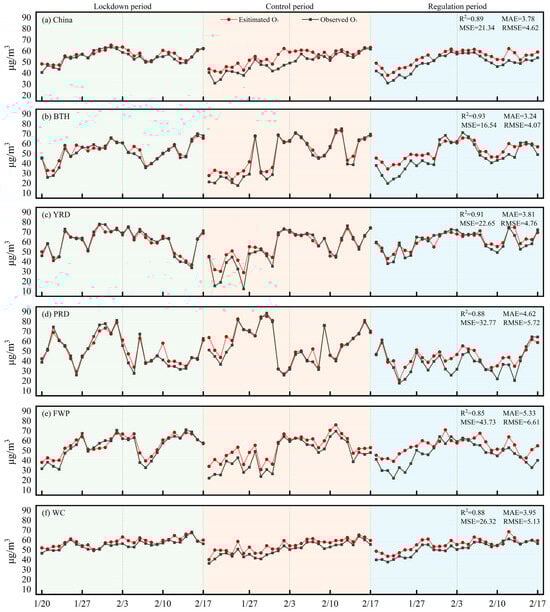
Figure 3.
Time series of O3 estimates (red) and observations (black) for (a) China and (b–f) five typical regions during the study period. R2, MAE, MSE, and RMSE for validation results of O3 in each region are given in the upper right corner.
3.2. Spatiotemporal Differences of XGBoost Model Surface O3 Estimation
Figure 3 also illustrates the time series of surface O3 for China and typical regions. The model exhibited strong responsiveness to short-term O3 pollution events. During the LP, surface O3 levels across China showed an overall increasing trend, ranging from 47.25 to 73.89 μg/m3. O3 levels in BTH, YRD, and FWP exhibited fluctuating increases, whereas the PRD experienced exceptionally large variations. In contrast, the WC remained relatively stable. In February 2021, northern China experienced a sharp rise in O3 concentration, whereas a steep drop of 48.36 μg/m3 (147.8%) occurred in PRD from 1st February to 2nd. Unlike other regions, the PRD exhibited recurrent downward trends in O3 during the RP. Meanwhile, the WC demonstrated no notable variations, suggesting that emissions played a limited role in the region, while geographic and meteorological factors may have exerted a greater influence.
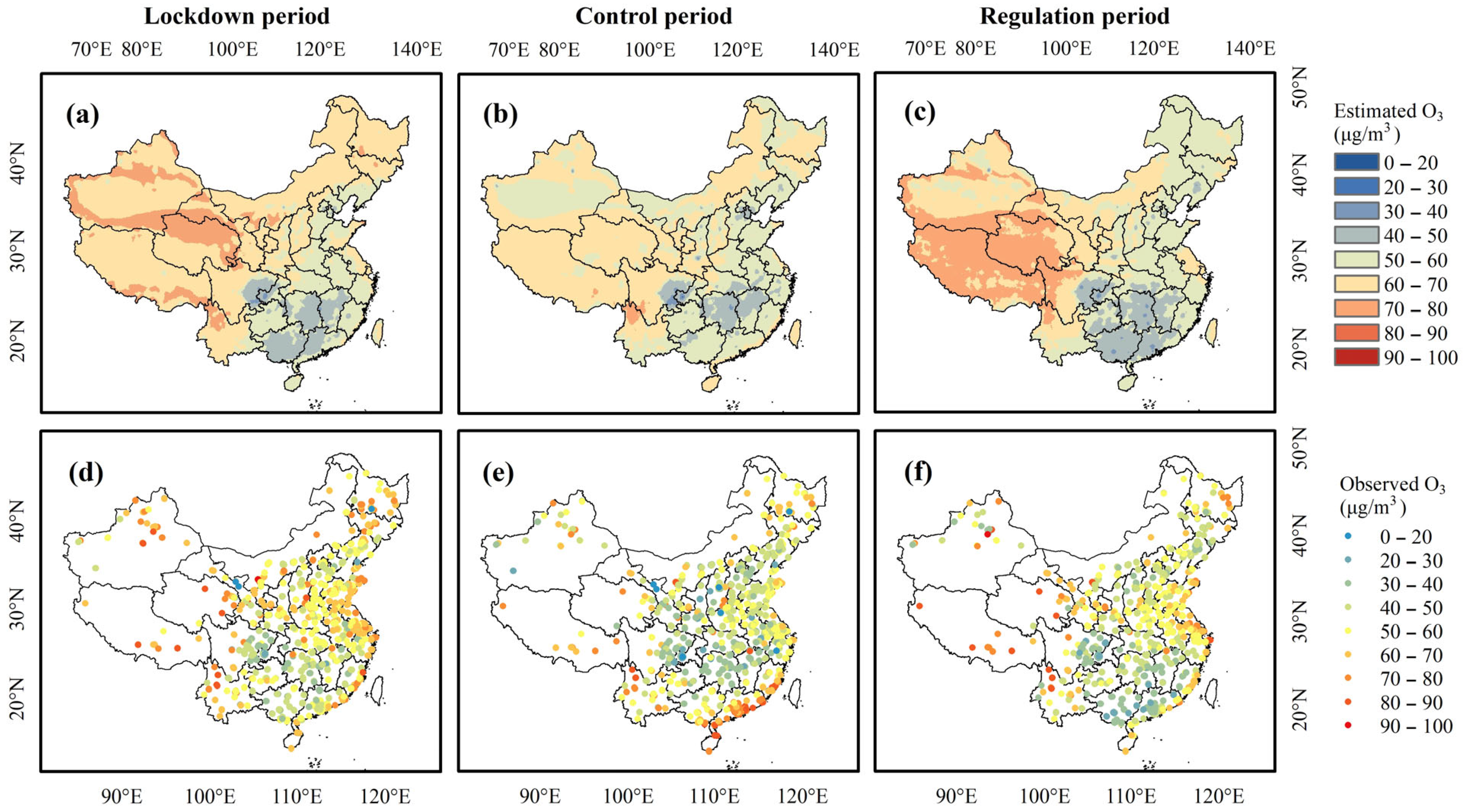
Based on the hourly surface O3 dataset generated by fusing multisource data with the XGBoost model, the spatial distribution of O3 at different stages of the COVID-19 period was mapped. Figure 4 displays the spatial consistency between observed O3 and estimated O3. The simulation results demonstrate that areas with high O3 levels were predominantly located in the north and WC, whereas southern China exhibited relatively lower O3 levels during the LP. Compared to the LP, the O3 decreased by 5.41% (3.21 μg/m3) as shown in the CP, primarily in WC such as Xinjiang, Tibet, and Qinghai. In contrast, O3 levels increased by 10–15 μg/m3 in Guangxi and Guangdong. Under regulatory measures in 2022, O3 decreased by 4.67% (2.79 μg/m3), primarily in eastern and southern China, with an average concentration of 59.79 μg/m3. However, significant increases in O3 levels were observed in Tibet and Qinghai. A notable O3 hotspot was found at the junction of northwest Yunnan and Sichuan, potentially influenced by stratospheric transport [61]. Due to the sparse distribution of monitoring stations, ground observations substantially underestimated O3 in WC, particularly during the CP. With the complete spatial coverage provided by the model, the estimated results revealed an average increase of 6.82 μg/m3 in O3 levels in WC. The WRF-Chem simulation results further validated the reliability of the estimated spatial distribution of surface O3 (Figure S2).
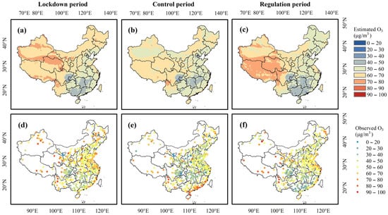
Figure 4.
(a–c) Spatial distributions of estimated O3 derived from XGBoost model, and (d–f) observed O3 during LP, CP, and RP.
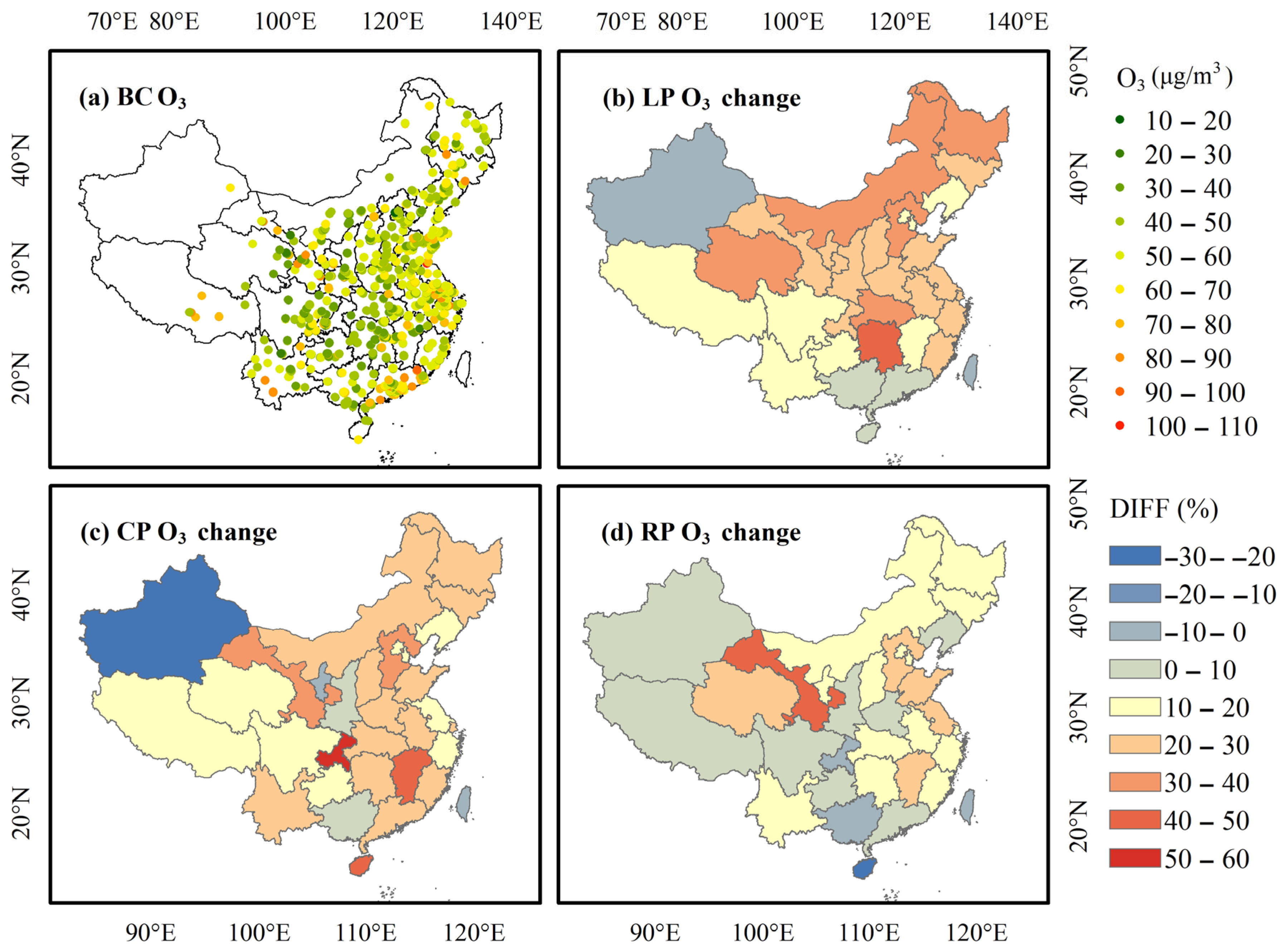
Figure 5 illustrates the fractional changes (DIFF) in surface O3 estimates across Chinese provinces between different stages of COVID-19 and BC. Compared to BC, surface O3 increased remarkably by 16.8% during the LP, predominantly in eastern (8.17 μg/m3) and central China (11.41 μg/m3) with DIFF of 22.64% and 23.84%, respectively. The northern region experienced greater changes than the southern region, with increases exceeding 40% in Hebei, Qinghai, Inner Mongolia, and Heilongjiang. These variations are considerably due to differences in NOx and VOCs ratios, changes in meteorology, and interactions with other pollutants [62]. Xinjiang was the only province exhibiting a decrease in O3 (−3.24%), which is likely attributed to an underestimation resulting from limited ground-based observations. During the CP, O3 increased across several southern provinces, with the highest rise of 35.17% in Chongqing. Although the national average O3 level was 4.21 μg/m3 higher than that in 2019, decreasing trends were observed in the FWP, central, and southern China. In contrast, O3 in WC increased by 14.38%, with Gansu DIFF increased by 43.3%. This increase was mainly attributed to olefin emissions from the petrochemical industry, which significantly contribute to elevated O3 levels [63].
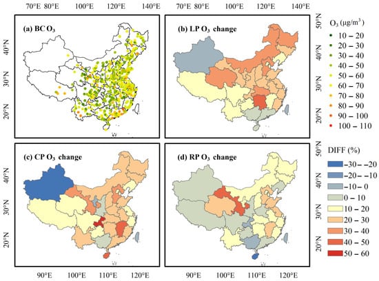
Figure 5.
(a) Spatial distribution of O3 observations during the BC. The DIFF in surface O3 across various Chinese provinces are obtained by the difference between BC and (b) LP, (c) CP, and (d) RP, where panels (b–d) are based on surface O3 estimates.
3.3. Spatial Analysis of the Short-Term Severe O3 Pollution Event
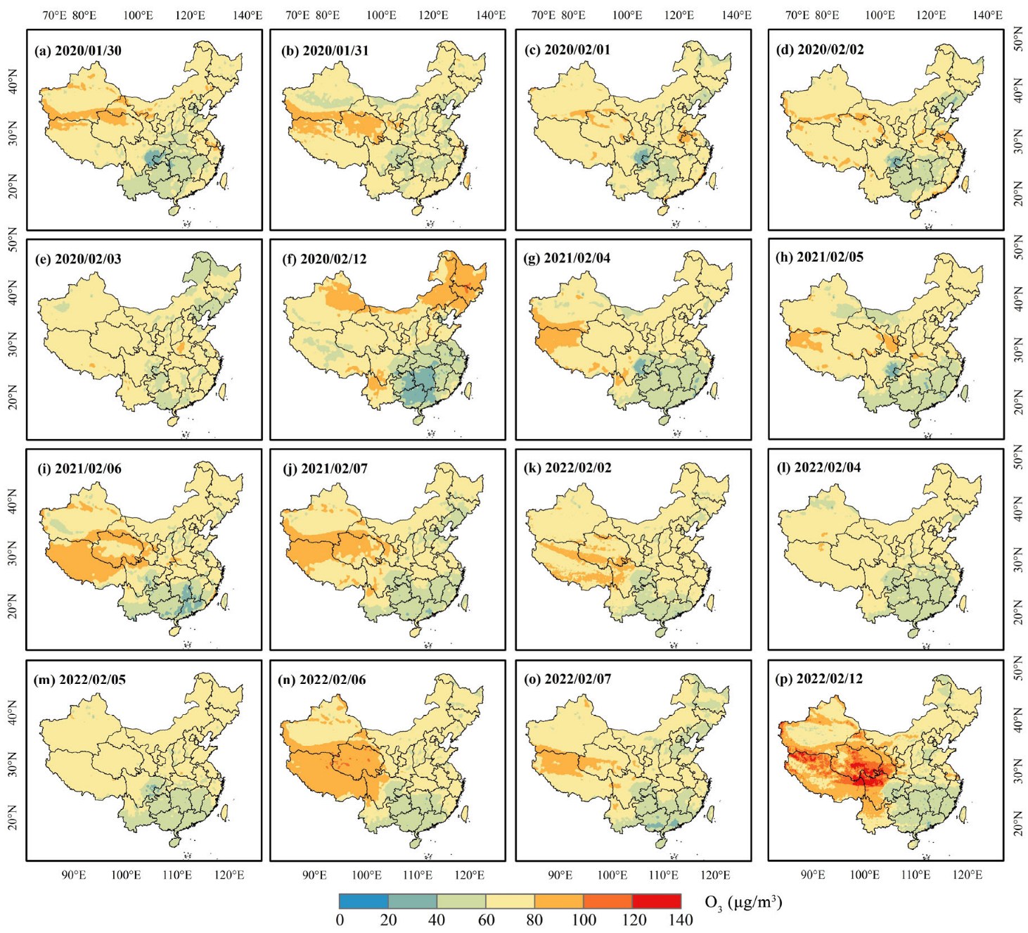
We also focused on typical cases with daily average O3 concentration above 65 μg/m3, while extreme values surpassed 100 μg/m3. Figure 6 illustrates the substantial daily variability in O3 distribution. Short-term O3 pollution events were mostly concentrated in February and exhibited uneven spatial distribution. High O3 value areas were distributed in the north and WC, with comparatively lower concentrations in the south. Wintertime coal heating in northern China sustained NOx saturation, whereas anthropogenic emissions in the south remained lower than in the north, even under strict lockdown policies. This regional disparity highlights the impact of heating practices on air pollution patterns [64]. However, abnormal variations may occur during certain periods. For instance, O3 hotspots formed in northeast China on 12 February 2020, contrasting with a sharp decline in O3 levels in southern China. Furthermore, daily O3 in eastern and central China showed minimal variation in February 2022, while the WC exhibited noticeably high O3 pollution levels (>120 μg/m3). The highest O3 level in WC was recorded on 12 February 2022.
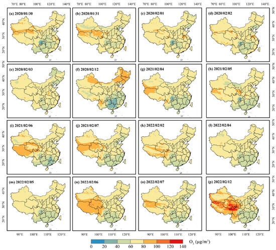
Figure 6.
Each subfigure represents the spatial distribution of daily average O3 concentration above 65 μg/m3 and extreme values surpassed 100 μg/m3. The corresponding date is indicated in the upper left corner.
3.4. Spatial Disparity Caused by Meteorology and Emission
Surface O3 formation depends on the influence of photochemical processes including precursors and meteorological conditions, and is generally divided into two distinct chemical properties: VOCs-sensitive and NOx-sensitive. We used the satellite-derived indicator FNR to characterize the sensitivity of surface O3 production. Species with similar lifetimes in the FNR (on the order of hours for NO2 and HCHO) better represent the interactions between the catalytic cycles that result in O3 production [65].
TROPOMI satellite observed NO2 of 0.03 mol m−3 during the LP, detailing a 30–40% decrease in contrast to the same period in 2019. More than 90% of regions were NOx-sensitive during this period, and urban areas exhibited VOCs-sensitive and transitional states (Figure 7). The reduction in NOx emissions decreased the NO2 available for photolysis, thereby decreasing the amount of free oxygen atoms available to form O3 [43]. Consequently, NO2 reduced substantially in areas dominated by urban agglomerations (e.g., BTH, YRD, PRD), resulting in a transition from NOx-limited to VOC-limited O3 generation sensitivity. When NOx reached a saturated state, the lockdown-induced reduction in NOx emissions weakened O3 depletion. Meanwhile, HCHO levels exhibited a uniform distribution, depicting minimal variations. As productivity approached normal in 2022, VOCs restrictions gradually shifted toward a transition state. Adjusting either a single emission or simultaneously reducing both precursors can effectively reduce O3 production in urban areas.
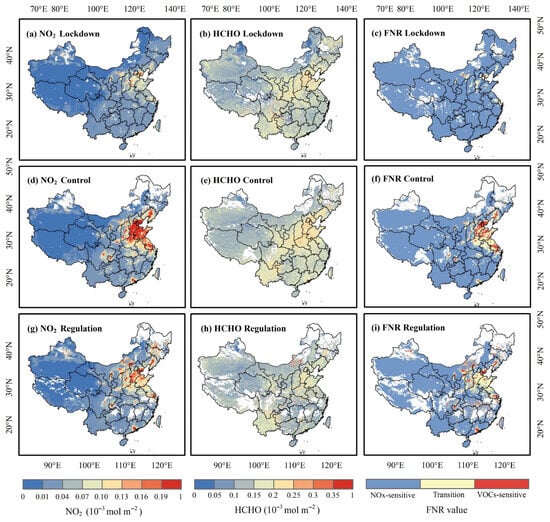
Figure 7.
The spatial distribution of TROPOMI NO2 (a,d,g), TROPOMI HCHO product (b,e,h), and the FNR (c,f,i) during LP, CP, and RP.
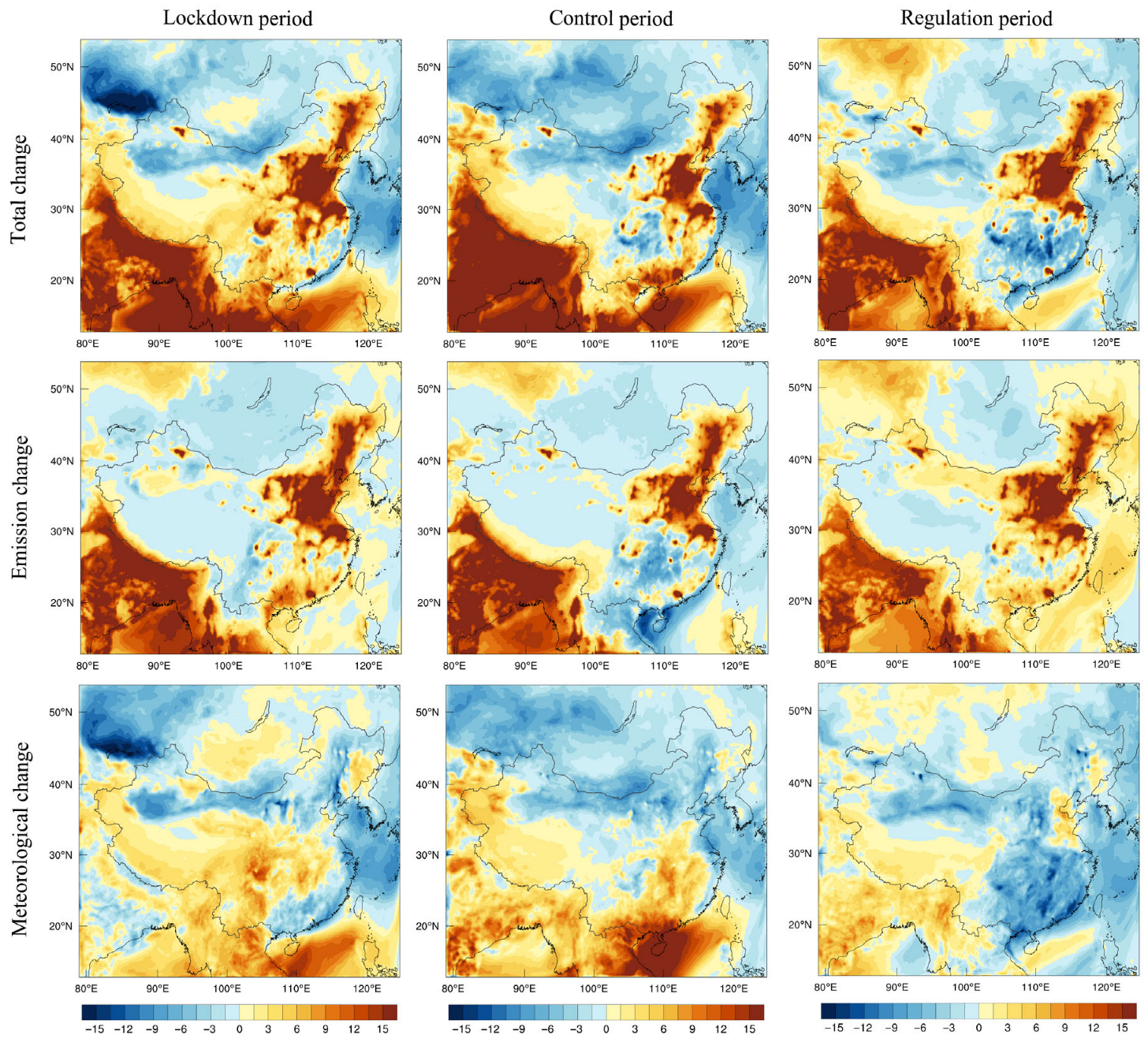
Based on the sensitivity simulations performed by WRF-Chem, the contribution of meteorological conditions and anthropogenic emissions to O3 levels in China is analyzed (Figure 8). Compared to previous model evaluations, the simulated values in this study showed a good correlation with observed values (R2 = 0.68–0.84, Table S2) and were suitable for further analysis (Table S3) [15,66,67,68]. During the LP, the combined contribution of meteorology and emissions to surface O3 increased by 4.06 μg/m3 compared to BC. Emissions from urban agglomerations led to an O3 increase of 9.06–15.96 μg/m3, which was partially offset by meteorological conditions (0.59–2.69 μg/m3). In contrast, meteorological contributions in FWP and WC contributed 5.70 μg/m3 and 1.57 μg/m3, respectively, which further exacerbated O3 pollution. It is noteworthy that O3 levels in the PRD increased by 71.7% during the CP, with contributions of 9.27 μg/m3 and 8.36 μg/m3 from emissions and meteorology, respectively (Table 4). Differently in other periods, both emissions and meteorological conditions contributed to an increase in O3. At this time, O3 sensitivity in the Pearl River Delta (PRD) was primarily VOC-limited and transitioning. This suggests that the unexpected rise in O3 levels in the PRD was not solely due to the disproportionate reduction in NOx and VOCs emissions but was also influenced by unfavorable meteorological conditions. During the RP, O3 pollution showed improvement across most regions, which can be attributed to reduced NOx emissions under transitional conditions, coupled with relatively stable VOC emission levels. However, anthropogenic emissions contributed significantly to O3 levels in the BTH (15.57 μg/m3). Based on the spatial distribution of O3 estimated by XGBoost, we found significant differences in O3 levels between WC and the South China region during the same period. During the LP and RP, emissions promoted O3 formation in South China, but favorable meteorological conditions effectively offset the increases caused by emissions. Conversely, meteorological conditions contributed to elevated O3 levels in WC throughout the COVID-19 pandemic, while emission reductions partially offset the concentration rise.
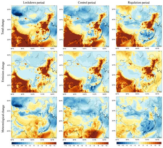
Figure 8.
Compared to the same period in 2019, O3 change over China is attributed to total change, meteorological variability, and emission changes during the LP, CP, RP as derived from WRF-Chem.
Table 4.
The impact of changes in O3 (Total), meteorological conditions (Met), and anthropogenic emissions (Emi) on O3 levels over China and five representative regions.
To understand the decision-making mechanism of the model, an interpretability analysis of variables was performed based on the SHAP algorithm. The SHAP value provides reasonable quantification of input variable contribution to O3 change, and explains the direction a feature contributes to a specific prediction [69]. During the COVID-19 period, solar radiation (UVB and SSR) ranked first in both the importance ranking and SHAP values, indicating that such features were highly important and had a significant positive impact on O3 (Figure 9). As solar radiation increases, O3 also rises accordingly. Despite weaker solar radiation in winter, it still serves as a main driving force for photochemical reactions in the atmosphere [23]. Temperature has a negative impact on O3, which is attributed to the weak atmospheric instability and temperature inversions in winter that restrict vertical air mixing, leading to the accumulation of O3 in the lower atmosphere. Furthermore, under the interaction of lower temperatures, high humidity inhibits surface O3 depletion [70]. NOx received a relatively low importance score in the model but showed a high SHAP value, indicating that although it was not frequently used during model training, it had a significant negative effect on O3, with contributions of −3.77 and −4.44 during the CP and RP, respectively. During the LP, NOx and TCO3 also exhibited high SHAP values. NOx emissions have dropped significantly under the background of low human activities, which has weakened the titration effect and led to the rapid accumulation of O3. High O3 concentrations have enhanced the oxidation of the atmospheric environment and intensified other photochemical reactions [71]. VOCs emerged as an important variable during the RP. O3 production takes place by photochemical oxidation of VOCs in the presence of NOx, catalyzed by hydroxyl radicals [72]. However, the SHAP values for NOx were notably higher than those for VOCs across all stages, implying that O3 formation was highly sensitive to NOx.
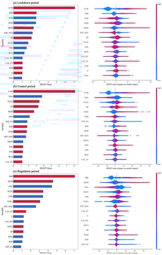
Figure 9.
The top 15 important features ranked by SHAP value are presented in (a) LP, (b) CP, and (c) RP. The left column shows the feature importance of different variables based on interpretability of the model. The right column illustrates the SHAP importance scores of summary plot.
4. Discussion
4.1. Comparison with Other O3 Modeling
This study establishes an hourly seamless dataset of surface O3 in China based on machine learning and multisource data. The results indicate that the model achieves high accuracy and effectively fills data gaps. Compared to satellite and ground-based monitoring products, the hourly surface O3 maps generated using the XGBoost model exhibit superior spatial coverage. A comparison between O3 model performance reported in previous studies and that of our model is provided in Table 5. Most previous studies have focused on daily O3 estimation using ML, but reported R2 values generally below 0.90. With advances in technology and computational capabilities, recent studies have improved the temporal resolution of O3 estimation to the hourly scale. Yang et al. constructed a multioutput random forest model and achieved estimation of hourly O3 in China, with sample-based CV-R2 reaching 0.94. Gao et al. showed hourly ML-derived O3 with R2 values exceeding 0.95 and RMSE below 7.50 μg/m3. Li et al. utilized a geostationary satellite to retrieve hourly O3, achieving high accuracy (R2 = 0.94). In contrast, our model achieves the sample-based CV-R2 values of 0.96–0.97 at the hourly scale, which demonstrates that the model has superior performance. Furthermore, the blind test results yielded R2 values of 0.95–0.96, further explaining the robustness of the model. Overall, our model demonstrated superior estimation ability than that yielded by previous methods in terms of the various temporal scales.
Table 5.
Comparison with previous similar studies.
4.2. Differences in O3 Levels During Multistage COVID-19
Benefitting from the high-resolution comprehensive coverage of the surface O3 dataset, this study provides an evaluation of O3 differences during the multistage COVID-19 pandemic, whereas previous research has mainly focused on the early stage of the outbreak. We found that significant variations in O3 distribution were observed at different stages, and short-term O3 pollution events exhibited marked spatiotemporal heterogeneity on a daily scale. No abnormal diurnal patterns or intensification of daily O3 cycles were detected during pollution events (Figure S3), and thus no further analysis was conducted. Nevertheless, the result can demonstrate that the estimated hourly O3 is basically consistent with the observed O3.
In addition, we quantify the contribution of winter meteorology and emissions to O3. WRF-Chem aims to separate the effects of meteorology and emissions, while SHAP refines the contribution levels of specific factors. WRF-Chem reveals the complexity of O3 generation in different regions. The emission reductions after the lockdown weakened the urban NOx titration, resulting in increased O3 levels. Unfavorable meteorological conditions offset the benefits of emission reductions in FWP and WC. The contribution of emissions to O3 declined during the CP, and more urban areas shifted from NOx restrictions to VOC restriction. The rise of urban O3 is attributed to increased VOCs and reduced NOx emissions under VOC-limited conditions. Meanwhile, the reduction in NOx and the relative stability of VOCs under the transitional state slowed down the O3 increases during the RP. Moreover, O3 shows strong sensitivity to meteorological changes in PRD and WC.
4.3. Uncertainty Analysis
One limitation of this study is that the use of high-resolution modeling and rigorous evaluation methods for estimating hourly O3 has increased the computational cost. As a result, the surface O3 dataset was constructed only for the COVID-19 period. Although the study spans three years, the temporal coverage remains relatively limited. In addition, we obtained good prediction results for a limited number of stations in WC, indicating that the model has strong spatial prediction capabilities. However, the accuracy of estimates in regions lacking monitoring stations remains uncertain. To validate the accuracy of O3 estimates in data-sparse regions with limited monitoring stations, acquiring additional ground-based observations remains crucial for model refinement and evaluation. Future studies could extend the model to longer time periods and incorporate additional observational data from the WC for validation.
5. Conclusions
This study used the XGBoost algorithm to fuse multisource data and establish an hourly full coverage surface O3 dataset over China. The results indicate that the optimized model demonstrated higher accuracy, with CV-R2 of 0.96–0.97 and RMSE of 4.58–5.00 μg/m3. In addition, the blind test yielded CV-R2 of 0.95–0.96 and RMSE of 20.98–30.10 μg/m3, further confirming the model’s robustness and reliability. In terms of temporal performance and spatial prediction capability, the results in China and typical regions further highlight the superior accuracy and reliability of our model (R2 = 0.85–0.93; RMSE = 4.07–6.61 μg/m3). Moreover, the model effectively fills spatial data gaps and corrects O3 underestimation. O3 increased by 16.8% during the LP compared to 2019, with high concentrations mainly distributed in the north and west, while lower levels were concentrated in the south. Additionally, O3 levels decreased by 5.41% during the CP and declined further under the regulatory measures implemented in 2022. Throughout the COVID-19 period, solar radiation significantly influenced O3 levels, and NOx also showed a strong association with O3, particularly during the CP and RP. Meteorological changes can either aggravate or alleviate O3 levels, but anthropogenic emissions play a crucial role in O3 formation. It is essential to simultaneously regulate the emission reduction ratios of O3 precursors while considering the meteorological conditions in PRD and WC.
Supplementary Materials
The following supporting information can be downloaded at: https://www.mdpi.com/article/10.3390/rs17132318/s1, Figure S1: Features correlation heatmap of O3 and variables in (a) LP, (b) CP and (c) RP; Figure S2: Spatial distribution of O3 during the (a) Base, (b) Base_LP, (b) Base_CP, and (b) Base_RP as derived from WRF-Chem over China; Figure S3: Time series of estimated O3 and observed O3 from 30 January to 4 February 2020; Table S1: WRF-Chem model configurations.; Table S2: The average O3 concentrations (μg/m3) from O3 observation, WRF-Chem and XGBoost model in China, and evaluation of the simulated WRF-Chem and ground-based observations; Table S3: Comparative evaluation of surface O3 (μg/m3) simulation performance.
Author Contributions
Writing–original draft, J.F., writing—review and editing: T.W., U.K., Software: J.F., T.W., methodology, J.F., data curation: J.F., conceptualization: T.W., resources: T.W., funding acquisition: T.W., visualization: J.F., Q.W., validation: J.F., Q.W., S.L., B.Z., investigation: Q.W., M.L., M.X. All authors have read and agreed to the published version of the manuscript.
Funding
This work was supported by the National Natural Science Foundation of China (42477103, 42077192). The authors are grateful for the support of the National Key Basic Research Development Program of China (2024YFC3711905, 2020YFA0607802). This work was supported by the Postgraduate Research & Practice Innovation Program of Jiangsu Province (KYCX25_0348).
Data Availability Statement
The data presented in this study are available on request from the corresponding author.
Conflicts of Interest
The authors declare that they have no known competing financial interests or personal relationships that could have appeared to influence the work reported in this paper.
Abbreviations
The following abbreviations are used in this manuscript:
| UVB | Downward UV radiation |
| BLH | Planetary boundary layer height |
| T2M | 2 m temperature |
| D2M | 2 m dewpoint temperature |
| E | Evaporation |
| LAI_HV | Leaf area index, high vegetation |
| LAI_LV | Leaf area index, low vegetation |
| ASN | Snow albedo |
| SP | Surface pressure |
| SSR | Surface net solar radiation |
| STR | Surface net thermal radiation |
| ASN | Snow albedo |
| TSN | Temperature of snow layer |
| TCO3 | Total column ozone |
| TP | Total precipitation |
| U10 | 10 m eastward wind |
| V10 | 10 m northward wind |
References
- Gharibzadeh, M.; Bidokhti, A.A.; Alam, K. The interaction of ozone and aerosol in a semi-arid region in the Middle East: Ozone formation and radiative forcing implications. Atmos. Environ. 2021, 245, 118015. [Google Scholar] [CrossRef]
- Ito, K.; De Leon, S.F.; Lippmann, M. Associations Between Ozone and Daily Mortality: Analysis and Meta-Analysis. Epidemiology 2005, 16, 446–457. [Google Scholar] [CrossRef] [PubMed]
- Emberson, L.D.; Pleijel, H.; Ainsworth, E.A.; Berg, M.v.D.; Ren, W.; Osborne, S.; Mills, G.; Pandey, D.; Dentener, F.; Büker, P.; et al. Ozone effects on crops and consideration in crop models. Eur. J. Agron. 2018, 100, 19–34. [Google Scholar] [CrossRef]
- Sillmann, J.; Aunan, K.; Emberson, L.; Bueker, P.; Van Oort, B.; OnEill, C.; Otero, N.; Pandey, D.; Brisebois, A. Combined impacts of climate and air pollution on human health and agricultural productivity. Environ. Res. Lett. 2021, 16, 093004. [Google Scholar] [CrossRef]
- Lu, X.; Hong, J.; Zhang, L.; Cooper, O.R.; Schultz, M.G.; Xu, X.; Wang, T.; Gao, M.; Zhao, Y.; Zhang, Y. Severe Surface Ozone Pollution in China: A Global Perspective. Environ. Sci. Technol. Lett. 2018, 5, 487–494. [Google Scholar] [CrossRef]
- Li, M.; Huang, X.; Yan, D.; Lai, S.; Zhang, Z.; Zhu, L.; Lu, Y.; Jiang, X.; Wang, N.; Wang, T.; et al. Coping with the concurrent heatwaves and ozone extremes in China under a warming climate. Sci. Bull. 2024, 69, 2938–2947. [Google Scholar] [CrossRef]
- Lu, X.; Zhang, L.; Wang, X.; Gao, M.; Li, K.; Zhang, Y.; Yue, X.; Zhang, Y. Rapid Increases in Warm-Season Surface Ozone and Resulting Health Impact in China Since 2013. Environ. Sci. Technol. Lett. 2020, 7, 240–247. [Google Scholar] [CrossRef]
- Zhu, J.; Chen, L.; Liao, H.; Yang, H.; Yang, Y.; Yue, X. Enhanced PM2.5 Decreases and O3 Increases in China During COVID-19 Lockdown by Aerosol-Radiation Feedback. Geophys. Res. Lett. 2021, 48, e2020GL090260. [Google Scholar] [CrossRef]
- Zuo, P.; Zong, Z.; Zheng, B.; Bi, J.; Zhang, Q.; Li, W.; Zhang, J.; Yang, X.; Chen, Z.; Yang, H.; et al. New Insights into Unexpected Severe PM2.5 Pollution during the SARS and COVID-19 Pandemic Periods in Beijing. Environ. Sci. Technol. 2022, 56, 155–164. [Google Scholar] [CrossRef]
- Xia, C.; Liu, C.; Cai, Z.; Duan, X.; Hu, Q.; Zhao, F.; Liu, H.; Ji, X.; Zhang, C.; Liu, Y. Improved Anthropogenic SO2 Retrieval from High-Spatial-Resolution Satellite and its Application during the COVID-19 Pandemic. Environ. Sci. Technol. 2021, 55, 11538–11548. [Google Scholar] [CrossRef]
- Cooper, M.J.; Martin, R.V.; Hammer, M.S.; Levelt, P.F.; Veefkind, P.; Lamsal, L.N.; Krotkov, N.A.; Brook, J.R.; McLinden, C.A. Global fine-scale changes in ambient NO2 during COVID-19 lockdowns. Nature 2022, 601, 380–387. [Google Scholar] [CrossRef] [PubMed]
- Kroll, J.H.; Heald, C.L.; Cappa, C.D.; Farmer, D.K.; Fry, J.L.; Murphy, J.G.; Steiner, A.L. The complex chemical effects of COVID-19 shutdowns on air quality. Nat. Chem. 2020, 12, 777–779. [Google Scholar] [CrossRef] [PubMed]
- Dutheil, F.; Baker, J.S.; Navel, V. COVID-19 as a factor influencing air pollution? Environ. Pollut. 2020, 263, 114466. [Google Scholar] [CrossRef]
- Monks, P.S.; Archibald, A.T.; Colette, A.; Cooper, O.; Coyle, M.; Derwent, R.; Fowler, D.; Granier, C.; Law, K.S.; Mills, G.E.; et al. Tropospheric ozone and its precursors from the urban to the global scale from air quality to short-lived climate forcer. Atmos. Chem. Phys. 2015, 15, 8889–8973. [Google Scholar] [CrossRef]
- Ryu, Y.; Hodzic, A.; Descombes, G.; Hu, M.; Barré, J. Toward a Better Regional Ozone Forecast Over CONUS Using Rapid Data Assimilation of Clouds and Meteorology in WRF-Chem. J. Geophys. Res. Atmos. 2019, 124, 13576–13592. [Google Scholar] [CrossRef]
- Neiburger, M. the role of meteorology in the study and control of air pollution. Bull. Am. Meteorol. Soc. 1969, 50, 957–966. [Google Scholar] [CrossRef]
- Sicard, P.; De Marco, A.; Agathokleous, E.; Feng, Z.; Xu, X.; Paoletti, E.; Rodriguez, J.J.D.; Calatayud, V. Amplified ozone pollution in cities during the COVID-19 lockdown. Sci. Total. Environ. 2020, 735, 139542. [Google Scholar] [CrossRef] [PubMed]
- Gettelman, A.; Lamboll, R.; Bardeen, C.G.; Forster, P.M.; Watson-Parris, D. Climate Impacts of COVID-19 Induced Emission Changes. Geophys. Res. Lett. 2021, 48, e2020GL091805. [Google Scholar] [CrossRef]
- Yan, D.; Jin, Z.; Zhou, Y.; Li, M.; Zhang, Z.; Wang, T.; Zhuang, B.; Li, S.; Xie, M. Anthropogenically and meteorologically modulated summertime ozone trends and their health implications since China’s clean air actions. Environ. Pollut. 2024, 343, 123234. [Google Scholar] [CrossRef]
- Filonchyk, M.; Hurynovich, V.; Yan, H.; Yang, S. Atmospheric pollution assessment near potential source of natural aerosols in the South Gobi Desert region, China. GIScience Remote. Sens. 2020, 57, 227–244. [Google Scholar] [CrossRef]
- Krotkov, N.A.; McLinden, C.A.; Li, C.; Lamsal, L.N.; Celarier, E.A.; Marchenko, S.V.; Swartz, W.H.; Bucsela, E.J.; Joiner, J.; Duncan, B.N.; et al. Aura OMI observations of regional SO2 and NO2 pollution changes from 2005 to 2015. Atmos. Chem. Phys. 2016, 16, 4605–4629. [Google Scholar] [CrossRef]
- Kwon, H.-A.; Park, R.J.; Jeong, J.I.; Lee, S.; Abad, G.G.; Kurosu, T.P.; Palmer, P.I.; Chance, K. Sensitivity of formaldehyde (HCHO) column measurements from a geostationary satellite to temporal variation of the air mass factor in East Asia. Atmos. Meas. Tech. 2017, 17, 4673–4686. [Google Scholar] [CrossRef]
- Wei, J.; Li, Z.; Li, K.; Dickerson, R.R.; Pinker, R.T.; Wang, J.; Liu, X.; Sun, L.; Xue, W.; Cribb, M. Full-coverage mapping and spatiotemporal variations of ground-level ozone pollution from 2013 to 2020 across China. Remote. Sens. Environ. 2022, 270, 112775. [Google Scholar] [CrossRef]
- Chen, B.; Hu, J.; Wang, Y. Synergistic observation of FY-4A&4B to estimate CO concentration in China: Combining interpretable machine learning to reveal the influencing mechanisms of CO variations. npj Clim. Atmos. Sci. 2024, 7, 9. [Google Scholar] [CrossRef]
- Shen, Y.; de Hoogh, K.; Schmitz, O.; Clinton, N.; Tuxen-Bettman, K.; Brandt, J.; Christensen, J.H.; Frohn, L.M.; Geels, C.; Karssenberg, D.; et al. Europe-wide air pollution modeling from 2000 to 2019 using geographically weighted regression. Environ. Int. 2022, 168, 107485. [Google Scholar] [CrossRef]
- Pernak, R.; Alvarado, M.; Lonsdale, C.; Mountain, M.; Hegarty, J.; Nehrkorn, T. Forecasting Surface O3 in Texas Urban Areas Using Random Forest and Generalized Additive Models. Aerosol Air Qual. Res. 2019, 9, 2815–2826. [Google Scholar] [CrossRef]
- Lee, S.; Park, S.; Lee, M.; Kim, G.; Im, J.; Song, C. Air Quality Forecasts Improved by Combining Data Assimilation and Machine Learning With Satellite AOD. Geophys. Res. Lett. 2022, 49, e2021GL096066. [Google Scholar] [CrossRef]
- Gao, Y.; Wang, Z.; Li, C.-Y.; Zheng, T.; Peng, Z.-R. Assessing neighborhood variations in ozone and PM2.5 concentrations using decision tree method. Build. Environ. 2021, 188, 107479. [Google Scholar] [CrossRef]
- Olson, D.A.; Riedel, T.P.; Offenberg, J.H.; Lewandowski, M.; Long, R.; Kleindienst, T.E. Quantifying wintertime O3 and NOx formation with relevance vector machines. Atmos. Environ. 2021, 259, 118538. [Google Scholar] [CrossRef]
- Lovrić, M.; Pavlović, K.; Vuković, M.; Grange, S.K.; Haberl, M.; Kern, R. Understanding the true effects of the COVID-19 lockdown on air pollution by means of machine learning. Environ. Pollut. 2021, 274, 115900. [Google Scholar] [CrossRef]
- Sun, H.; Shin, Y.M.; Xia, M.; Ke, S.; Wan, M.; Yuan, L.; Guo, Y.; Archibald, A.T. Spatial Resolved Surface Ozone with Urban and Rural Differentiation during 1990–2019: A Space–Time Bayesian Neural Network Downscaler. Environ. Sci. Technol. 2022, 56, 7337–7349. [Google Scholar] [CrossRef] [PubMed]
- Zhan, Y.; Luo, Y.Z.; Deng, X.F.; Grieneisen, M.L.; Zhang, M.H.; Di, B.F. Spatiotemporal prediction of daily ambient ozone levels across China using random forest for human exposure assessment. Environ. Pollut. 2018, 233, 464–473. [Google Scholar] [CrossRef] [PubMed]
- Li, R.; Cui, L.; Hongbo, F.; Li, J.; Zhao, Y.; Chen, J. Satellite-based estimation of full-coverage ozone (O3) concentration and health effect assessment across Hainan Island. J. Clean. Prod. 2020, 244, 118773. [Google Scholar] [CrossRef]
- Wang, H.; Wang, H.; Lu, X.; Lu, K.; Zhang, L.; Tham, Y.J.; Shi, Z.; Aikin, K.; Fan, S.; Brown, S.S.; et al. Increased night-time oxidation over China despite widespread decrease across the globe. Nat. Geosci. 2023, 16, 217–223. [Google Scholar] [CrossRef]
- Veefkind, J.P.; Aben, I.; McMullan, K.; Förster, H.; de Vries, J.; Otter, G.; Claas, J.; Eskes, H.J.; de Haan, J.F.; Kleipool, Q.; et al. TROPOMI on the ESA Sentinel-5 Precursor: A GMES mission for global observations of the atmospheric composition for climate, air quality and ozone layer applications. Remote Sens. Environ. 2012, 120, 70–83. [Google Scholar] [CrossRef]
- van Geffen, J.; Boersma, K.F.; Eskes, H.; Sneep, M.; Ter Linden, M.; Zara, M.; Veefkind, J.P. S5P TROPOMI NO2 slant column retrieval: Method, stability, uncertainties and comparisons with OMI. Atmos. Meas. Tech. 2020, 13, 1315–1335. [Google Scholar] [CrossRef]
- Su, W.; Liu, C.; Chan, K.L.; Hu, Q.; Liu, H.; Ji, X.; Zhu, Y.; Liu, T.; Zhang, C.; Chen, Y.; et al. An improved TROPOMI tropospheric HCHO retrieval over China. Atmos. Meas. Tech. 2020, 13, 6271–6292. [Google Scholar] [CrossRef]
- De Smedt, I.; Pinardi, G.; Vigouroux, C.; Compernolle, S.; Bais, A.; Benavent, N.; Boersma, F.; Chan, K.-L.; Donner, S.; Eichmann, K.-U.; et al. Comparative assessment of TROPOMI and OMI formaldehyde observations and validation against MAX-DOAS network column measurements. Atmos. Chem. Phys. 2021, 21, 12561–12593. [Google Scholar] [CrossRef]
- Levelt, P.F.; Joiner, J.; Tamminen, J.; Veefkind, J.P.; Bhartia, P.K.; Zweers, D.C.S.; Duncan, B.N.; Streets, D.G.; Eskes, H.; Van Der A, R.; et al. The Ozone Monitoring Instrument: Overview of 14 years in space. Atmos. Chem. Phys. 2018, 18, 5699–5745. [Google Scholar] [CrossRef]
- Mao, Y.; Wang, H.; Jiang, F.; Feng, S.; Jia, M.; Ju, W. Anthropogenic NOx emissions of China, the U.S. and Europe from 2019 to 2022 inferred from TROPOMI observations. Environ. Res. Lett. 2024, 19, 054024. [Google Scholar] [CrossRef]
- Palmer, P.I.; Jacob, D.J.; Fiore, A.M.; Martin, R.V.; Chance, K.; Kurosu, T.P. Mapping isoprene emissions over North America using formaldehyde column observations from space. J. Geophys. Res. Atmos. 2003, 108, e2002JD002153. [Google Scholar] [CrossRef]
- Sillman, S. The use of NO, H2O2, and HNO3 as indicators for O3-NO-hydrocarbon sensitivity in urban locations. J. Geophys. Res. Atmos. 1995, 100, 14175–14188. [Google Scholar] [CrossRef]
- Jin, X.; Holloway, T. Spatial and temporal variability of ozone sensitivity over China observed from the Ozone Monitoring Instrument. J. Geophys. Res. Atmos. 2015, 120, 7229–7246. [Google Scholar] [CrossRef]
- Badia, A.; Vidal, V.; Ventura, S.; Curcoll, R.; Segura, R.; Villalba, G. Modelling the impacts of emission changes on O3 sensitivity, atmospheric oxidation capacity and pollution transport over the Catalonia region. EGUsphere 2023, 23, 10751–10774. [Google Scholar] [CrossRef]
- Duncan, B.N.; Yoshida, Y.; Olson, J.R.; Sillman, S.; Martin, R.V.; Lamsal, L.; Hu, Y.; Pickering, K.E.; Retscher, C.; Allen, D.J.; et al. Application of OMI observations to a space-based indicator of NOx and VOC controls on surface ozone formation. Atmos. Environ. 2010, 44, 2213–2223. [Google Scholar] [CrossRef]
- Gerges, F.; Llaguno-Munitxa, M.; Zondlo, M.A.; Boufadel, M.C.; Bou-Zeid, E. Weather and the City: Machine Learning for Predicting and Attributing Fine Scale Air Quality to Meteorological and Urban Determinants. Environ. Sci. Technol. 2024, 58, 6313–6325. [Google Scholar] [CrossRef]
- Wei, J.; Li, Z.; Lyapustin, A.; Wang, J.; Dubovik, O.; Schwartz, J.; Sun, L.; Li, C.; Liu, S.; Zhu, T. First close insight into global daily gapless 1 km PM2.5 pollution, variability, and health impact. Nat. Commun. 2023, 14, 1–11. [Google Scholar] [CrossRef]
- Rodriguez, J.D.; Perez, A.; Lozano, J.A. Sensitivity Analysis of k-Fold Cross Validation in Prediction Error Estimation. IEEE Trans. Pattern Anal. Mach. Intell. 2010, 32, 569–575. [Google Scholar] [CrossRef] [PubMed]
- Grell, G.A.; Peckham, S.E.; Schmitz, R.; McKeen, S.A.; Frost, G.; Skamarock, W.C.; Eder, B. Fully coupled “online” chemistry within the WRF model. Atmos. Environ. 2005, 39, 6957–6975. [Google Scholar] [CrossRef]
- Lin, Y.L.; Farley, R.D.; Orville, H.D. Orville, Bulk Parameterization of the Snow Field in a Cloud Model. J. Appl. Meteorol. Climatol. 1983, 22, 1065–1092. [Google Scholar] [CrossRef]
- Mlawer, E.J.; Taubman, S.J.; Brown, P.D.; Iacono, M.J.; Clough, S.A. Radiative transfer for inhomogeneous atmospheres: RRTM, a validated correlated-k model for the longwave. J. Geophys. Res. Atmos. 1997, 102, 16663–16682. [Google Scholar] [CrossRef]
- Zhao, Q.; Carr, F.H. A Prognostic Cloud Scheme for Operational NWP Models. Mon. Weather. Rev. 1997, 125, 1931–1953. [Google Scholar] [CrossRef]
- Chen, F.; Dudhia, J. Coupling an Advanced Land Surface–Hydrology Model with the Penn State–NCAR MM5 Modeling System. Part I: Model Implementation and Sensitivity. Mon. Weather. Rev. 2001, 129, 569–585. [Google Scholar] [CrossRef]
- Janjić, Z.I. The Step-Mountain Eta Coordinate Model: Further Developments of the Convection, Viscous Sublayer, and Turbulence Closure Schemes. Mon. Weather. Rev. 1994, 122, 927–945. [Google Scholar] [CrossRef]
- Xu, K.; Cederwall, R.T.; Donner, L.J.; Grabowski, W.W.; Guichard, F.; Johnson, D.E.; Khairoutdinov, M.; Krueger, S.K.; Petch, J.C.; Randall, D.A.; et al. An intercomparison of cloud-resolving models with the atmospheric radiation measurement summer 1997 intensive observation period data. Q. J. R. Meteorol. Soc. 2002, 128, 593–624. [Google Scholar] [CrossRef]
- Stockwell, W.R.; Middleton, P.; Chang, J.S.; Tang, X. The second generation regional acid deposition model chemical mechanism for regional air quality modeling. J. Geophys. Res. Atmos. 1990, 95, 16343–16367. [Google Scholar] [CrossRef]
- Guenther, A.B.; Monson, R.K.; Fall, R. Isoprene and monoterpene emission rate variability: Observations with eucalyptus and emission rate algorithm development. J. Geophys. Res. Atmos. 1991, 96, 10799–10808. [Google Scholar] [CrossRef]
- Li, M.; Zhang, Q.; Zheng, B.; Tong, D.; Lei, Y.; Liu, F.; Hong, C.; Kang, S.; Yan, L.; Zhang, Y.; et al. Persistent growth of anthropogenic non-methane volatile organic compound (NMVOC) emissions in China during 1990–2017: Drivers, speciation and ozone formation potential. Atmos. Chem. Phys. 2019, 19, 8897–8913. [Google Scholar] [CrossRef]
- Tan, Z.; Feng, M.; Liu, H.; Luo, Y.; Li, W.; Song, D.; Tan, Q.; Ma, X.; Lu, K.; Zhang, Y. Atmospheric Oxidation Capacity Elevated during 2020 Spring Lockdown in Chengdu, China: Lessons for Future Secondary Pollution Control. Environ. Sci. Technol. 2024, 58, 8815–8824. [Google Scholar] [CrossRef]
- Wei, J.; Li, Z.; Lyapustin, A.; Sun, L.; Peng, Y.; Xue, W.; Su, T.; Cribb, M. Reconstructing 1-km-resolution high-quality PM2.5 data records from 2000 to 2018 in China: Spatiotemporal variations and policy implications. Remote. Sens. Environ. 2021, 252, 112136. [Google Scholar] [CrossRef]
- Lin, M.; Fiore, A.M.; Cooper, O.R.; Horowitz, L.W.; Langford, A.O.; Levy, H.; Johnson, B.J.; Naik, V.; Oltmans, S.J.; Senff, C.J. Springtime high surface ozone events over the western United States: Quantifying the role of stratospheric intrusions. J. Geophys. Res. Atmos. 2012, 117, e2012JD018151. [Google Scholar] [CrossRef]
- Le, T.; Wang, Y.; Liu, L.; Yang, J.; Yung, Y.L.; Li, G.; Seinfeld, J.H. Unexpected air pollution with marked emission reductions during the COVID-19 outbreak in China. Science 2020, 369, 702–706. [Google Scholar] [CrossRef] [PubMed]
- Yang, J.; Zeren, Y.; Guo, H.; Wang, Y.; Lyu, X.; Zhou, B.; Gao, H.; Yao, D.; Wang, Z.; Zhao, S.; et al. Wintertime ozone surges: The critical role of alkene ozonolysis. Environ. Sci. Ecotechnol. 2024, 22, 100477. [Google Scholar] [CrossRef] [PubMed]
- Liang, Y.; Gui, K.; Che, H.; Li, L.; Zheng, Y.; Zhang, X.; Zhang, X.; Zhang, P.; Zhang, X. Changes in aerosol loading before, during and after the COVID-19 pandemic outbreak in China: Effects of anthropogenic and natural aerosol. Sci. Total. Environ. 2023, 857, 159435. [Google Scholar] [CrossRef]
- Tonnesen, G.S.; Dennis, R.L. Analysis of radical propagation efficiency to assess ozone sensitivity to hydrocarbons and NO2. Long-lived species as indicators of ozone concentration sensitivity. J. Geophys. Res. Atmos. 2000, 105, 9227–9241. [Google Scholar] [CrossRef]
- Sun, J.; Shen, Z.; Wang, R.; Li, G.; Zhang, Y.; Zhang, B.; He, K.; Tang, Z.; Xu, H.; Qu, L.; et al. A comprehensive study on ozone pollution in a megacity in North China Plain during summertime: Observations, source attributions and ozone sensitivity. Environ. Int. 2021, 146, 106279. [Google Scholar] [CrossRef]
- Li, M.; Wang, T.; Shu, L.; Qu, Y.; Xie, M.; Liu, J.; Wu, H.; Kalsoom, U. Rising surface ozone in China from 2013 to 2017: A response to the recent atmospheric warming or pollutant controls? Atmos. Environ. 2021, 246, 118130. [Google Scholar] [CrossRef]
- Romero-Alvarez, J.; Lupaşcu, A.; Lowe, D.; Badia, A.; Acher-Nicholls, S.; Dorling, S.; Reeves, C.E.; Butler, T. Sources of surface O3 in the UK: Tagging O3 within WRF-Chem. Atmos. Chem. Phys. 2022, 22, 13797–13815. [Google Scholar] [CrossRef]
- Mai, Z.; Shen, H.; Zhang, A.; Sun, H.Z.; Zheng, L.; Guo, J.; Liu, C.; Chen, Y.; Wang, C.; Ye, J.; et al. Convolutional Neural Networks Facilitate Process Understanding of Megacity Ozone Temporal Variability. Environ. Sci. Technol. 2024, 58, 15691–15701. [Google Scholar] [CrossRef]
- Li, G.; Chen, Q.; Zhu, Y.; Sun, W.; Guo, W.; Zhang, R.; Zhu, Y.; She, J. Effects of chemical boundary conditions on simulated O3 concentrations in China and their chemical mechanisms. Sci. Total. Environ. 2023, 857, 159500. [Google Scholar] [CrossRef]
- Wang, H.; Liu, Y.; Chen, X.; Gao, Y.; Qiu, W.; Jing, S.; Wang, Q.; Lou, S.; Edwards, P.M.; Huang, C.; et al. Unexpected fast radical production emerges in cool seasons: Implications for ozone pollution control. Natl. Sci. Open 2022, 1, 13. [Google Scholar] [CrossRef]
- Li, K.; Jacob, D.J.; Liao, H.; Qiu, Y.; Shen, L.; Zhai, S.; Bates, K.H.; Sulprizio, M.P.; Song, S.; Lu, X.; et al. Ozone pollution in the North China Plain spreading into the late-winter haze season. Proc. Natl. Acad. Sci. USA 2021, 118, e2015797118. [Google Scholar] [CrossRef]
- Kang, Y.; Choi, H.; Im, J.; Park, S.; Shin, M.; Song, C.-K.; Kim, S. Estimation of surface-level NO2 and O3 concentrations using TROPOMI data and machine learning over East Asia. Environ. Pollut. 2021, 288, 117711. [Google Scholar] [CrossRef]
- Xiong, K.; Xie, X.; Huang, L.; Hu, J. Improved O3 predictions in China by combining chemical transport model and multi-source data with machining learning techniques. Atmos. Environ. 2024, 318, 120269. [Google Scholar] [CrossRef]
- Capilla, C. Prediction of hourly ozone concentrations with multiple regression and multilayer perceptron models. Int. J. Sustain. Dev. Plan. 2016, 11, 558–565. [Google Scholar] [CrossRef]
- Yang, Q.; Kim, J.; Cho, Y.; Lee, W.-J.; Lee, D.-W.; Yuan, Q.; Wang, F.; Zhou, C.; Zhang, X.; Xiao, X.; et al. A synchronized estimation of hourly surface concentrations of six criteria air pollutants with GEMS data. npj Clim. Atmos. Sci. 2023, 6, 94. [Google Scholar] [CrossRef]
- Chen, B.; Wang, Y.; Huang, J.; Zhao, L.; Chen, R.; Song, Z.; Hu, J. Estimation of near-surface ozone concentration and analysis of main weather situation in China based on machine learning model and Himawari-8 TOAR data. Sci. Total. Environ. 2023, 864, 160928. [Google Scholar] [CrossRef]
- Gao, L.; Zhang, H.; Yang, F.; Tan, W.; Wu, R.; Song, Y. First estimation of hourly full-coverage ground-level ozone from Fengyun-4A satellite using machine learning. Environ. Res. Lett. 2024, 19, 024040. [Google Scholar] [CrossRef]
- Li, S.; Song, G.; Xing, J.; Dong, J.; Zhang, M.; Fan, C.; Meng, S.; Yang, J.; Dong, L.; Gong, W. Unraveling overestimated exposure risks through hourly ozone retrievals from next-generation geostationary satellites. Nat. Commun. 2025, 16, 3364. [Google Scholar] [CrossRef]
- Xue, W.; Zhang, J.; Hu, X.; Yang, Z.; Wei, J. Hourly Seamless Surface O3 Estimates by Integrating the Chemical Transport and Machine Learning Models in the Beijing-Tianjin-Hebei Region. Int. J. Environ. Res. Public Health 2022, 19, 8511. [Google Scholar] [CrossRef]


Disclaimer/Publisher’s Note: The statements, opinions and data contained in all publications are solely those of the individual author(s) and contributor(s) and not of MDPI and/or the editor(s). MDPI and/or the editor(s) disclaim responsibility for any injury to people or property resulting from any ideas, methods, instructions or products referred to in the content. |
© 2025 by the authors. Licensee MDPI, Basel, Switzerland. This article is an open access article distributed under the terms and conditions of the Creative Commons Attribution (CC BY) license (https://creativecommons.org/licenses/by/4.0/).