1. Introduction
With the wide application of the global navigation satellite system (GNSS), its vulnerability has been gradually exposed [
1,
2,
3,
4]. As a navigation, positioning, and timing system independent of GNSS, the enhanced performance of the eLoran system plays an indispensable role in safeguarding national security, promoting economic development, and improving people’s quality of life [
5,
6,
7]. The eLoran system adopts long-wave signals to transmit time information, with strong anti-jamming ability, and its timing accuracy can meet the needs of most users [
8,
9]. It can also be used as an effective backup and supplementary system for the GNSS system [
10,
11,
12].
The current eLoran system generally adopts the differential technique to improve the timing accuracy of the system. Establishing an additional second time-delay factor (ASF) grid and using interpolation methods to calculate the ASF values within the grid is currently an effective method to improve the timing accuracy [
13]. However, changes in the meteorological environment can directly or indirectly lead to ASF fluctuations. Changes in meteorological factors can lead to changes in the electromagnetic environment of the radio wave propagation path, which affects the propagation characteristics of eLoran signals and is specifically quantified as fluctuations in propagation delay, affecting the timing accuracy of the eLoran system [
14].
In order to deal with the influence of meteorological factors on the eLoran system, it is necessary to deeply study the influence of changes in meteorological factors on signal propagation delay [
15]. By establishing the prediction model of eLoran signal propagation delay, the influence mechanism between meteorological factors and eLoran signal propagation delay was revealed. When the system malfunctions or the propagation path of the signal is affected by electromagnetic interference resulting in abnormal delay data, meteorological data can be utilized to predict the propagation delay. This technology provides a reliable guarantee for the stable timing of systems under complex meteorological conditions and electromagnetic interference environments, and at the same time promotes the development of long-wave meteorology, opening up new avenues for interdisciplinary integration.
The main research core of this thesis is to use meteorological data to predict the eLoran propagation delay data and to analyze the data of the influence mechanism of meteorological factors on the eLoran system at long distance. The 175 differential reference stations planned by the high precision ground-based timing system have the conditions to receive the propagation delay data accurately over long distances, which ensures the reliability of the data [
16,
17]. By 2022, the total number of national automatic weather stations reached 59,982. This large-scale and high-quality layout of weather stations is the core technical support for the development of this research [
18,
19].
The results show that the fluctuation in eLoran signal propagation delay is closely related to the quantitative changes in temperature and humidity, as well as the intensity of precipitation. The change in propagation delay with meteorological factors can be summarized into two main models: long-term seasonal cycle change and short-term weather fluctuation change. The former is usually closely related to cyclical factors, such as seasonal alternations. The latter reflects transient fluctuations in propagation delay affected by short-term weather conditions. The pioneering work on the correlation between eLoran signal propagation delay and meteorological factors can be traced back to 1985. McCollough J.R. et al. analyzed and processed a large number of measured data and concluded that the ASF showed significant seasonal variation characteristics [
20]. In 2010, Yang S.H. et al. proposed a compensation method after analyzing the daily variation data of temperature and humidity, which improved the prediction accuracy of eLoran signal propagation delay [
21]. Subsequently, Hwang S.W. and other scholars explained in detail the changes in the signal propagation environment, such as atmospheric refractive index and ground conductivity caused by temperature changes, and constructed a quantitative relationship model between temperature and propagation delay [
22]. In 2020, Wang et al. used the theoretical ASF data calculated by the integral equation method as the data source to train the BPNN model, and calibrated the BPNN model by the actual measured ASF data to improve the prediction accuracy of the model [
23]. Yang Hongjuan used multi-dimensional data to construct a neural network algorithm model and quantified the influence of meteorological factors on propagation delay [
24]. Liu Shiyao demonstrated that there is a complex and multi-dimensional nonlinear relationship between eLoran signal propagation delay and a variety of meteorological factors, established a multi-dimensional time-delay prediction model, and achieved good prediction accuracy [
25]. Although the current research in this field has made certain achievements, there are mainly the following problems at present: the research timespan is short, the space scope is limited, and the meteorological factors are relatively single. In view of the above shortcomings, the main contributions of this paper are as follows.
Firstly, the temporal and spatial differences of the influence of meteorological factors on the propagation delay of eLoran signals are studied: the long-term and short-term correlation between the signal propagation delay and the corresponding meteorological factors are compared and analyzed for the long-distance differential stations in the same path by using the path-weighted Pearson correlation method.
Secondly a multi-factor meteorological prediction model in long-distance scenarios is constructed: breaking through the limitation of linear model, the single-factor and multi-factor BP neural network prediction models are designed and compared, and the signal delay prediction is realized through multi-station data on temperature, humidity, and pressure.
3. Method Description
3.1. Influence of Meteorological Factors’ Fluctuation on Propagation Delay at Different Distances
From the previous analysis, it can be seen that the fluctuation of meteorological factors will make the propagation delay fluctuate. In this paper, the cumulative influence of meteorological factors fluctuation on propagation delay at different distances is analyzed from a theoretical perspective.
Assuming that the propagation path is a continuous curve, the fluctuation
of the total propagation delay is caused by the changes in meteorological factors (temperature
, humidity
, and pressure
) at each point on the path, and its fluctuation can be expressed as the cumulative effect of the changes in the meteorological factors on the path, as follows:
where
is a complex function of the time-delay fluctuation on a certain path micro-element, which cannot be given in an analytical form. The value of the function is related to the fluctuation in temperature, humidity, pressure, and other meteorological factors in addition to the propagation path length.
is the total propagation path length, while
,
,
are the variations in the meteorological factors at each point on the path.
When the propagation delay path is short, it can be considered that the meteorological parameters change approximately uniformly during each integration interval. Taking temperature as an example, when the propagation path is short and the path environment is similar, the temperature change trend of each road section of the propagation path also shows certain consistency, that is, the temperature of the whole path is heated or cooled in a short distance, and the average temperature change in the road section is assumed to be
, and the complex function of temperature’s influence on the time-delay fluctuation is replaced by
. Therefore, the effect of temperature on propagation delay should become increasingly important as the propagation path becomes longer, as in the following Equation (11):
When the propagation path changes from short-distance propagation to long-distance propagation, the change direction of meteorological factors on the propagation path is different in different regions. Take temperature as an example: In this case, the sign of
may change differently along the path in different regions, and the contributions of temperature in each region may cancel each other out. For example, a certain segment of
will contribute positively to the delay, and another segment of
will contribute negatively to the delay. May exhibit nonlinear or uncertain trends, or even decrease due to partial cancellation, as in the following Equation (12):
At this time, the positive and negative contributions of meteorological factors on each path of the total delay fluctuation in the summation process may cancel each other out, and the total delay trend is uncertain.
3.2. Correlation Analysis Methods in Long-Distance Scenarios
Because the influence mechanism of meteorological factors on eLoran signal propagation delay is complex, in order to find the meteorological factors with great influence on eLoran signal propagation delay, traditional statistical methods can be used to roughly measure the influence of meteorological factors on eLoran signal propagation delay. The literature [
25] shows that there is little difference in the results of using Pearson and the other three correlation coefficients to analyze the influence of meteorological factors on the propagation delay of eLoran signals. Due to space limitation in this paper, our correlation analysis only focuses on the Pearson correlation coefficient.
However, as the signal propagation distance becomes longer and longer, the meteorological conditions on the path are complex and changeable. Suppose that a certain differential reference station on the propagation path is cooled down one day, and other locations are warmed up. At this time, the length of the warmed road section is much larger than that of the cooled road section. According to the conclusion obtained from
Section 3.1, the contribution of temperature to the time-delay on the whole path is positive. In the case of short-distance propagation, it is correct to conclude that the relationship between temperature and propagation delay is a positive correlation. However, in the case of long-distance propagation, it is one-sided to use the temperature data of a certain weather station on the path to calculate the correlation coefficient and draw the conclusion that the propagation delay is negatively correlated with temperature on the path from Pucheng to the differential reference station. Therefore, it is necessary to consider the contribution difference of temperature in different road sections to the total delay, and a calculation method of the Pearson correlation coefficient based on distance weighting is proposed as follows.
Firstly, path segmentation and weight distribution are performed. We divide the propagation path into
segments with each corresponding to a weather station, and let the length of the
segment be
, and the total path length be as follows:
We define the weight of the path in segment
as in the following Formula (14):
Secondly, a weighted calculation of temperature is conducted. For each day, the temperature of each road section
is weighted and averaged according to the path to obtain the global temperature
:
where
is the temperature data of the corresponding weather station of the path in segment
.
Finally, the Pearson correlation coefficient calculation is conducted. We calculate the Pearson correlation coefficient between the weighted temperature series
and the propagation delay series d, as follows:
where
is the length of the propagation delay and temperature sequence, while
and
are the mean values of weighted temperature and propagation delay, respectively.
The algorithm uses the method of distance weighting to fuse the meteorological data of multiple weather stations and weight the temperature sequence by distance, so that the temperature change in the long section of the road contributes more to the total delay and gives it a higher weight, which effectively solves the problem of data one-sidedness caused by local temperature variation in the process of long-distance propagation. It more accurately depicts the temperature distribution on the whole path, which is more in line with the actual physical process. When the path is short, we set , and the Pearson coefficient degrades to the traditional Pearson coefficient. The derivation of the above algorithm is only based on the meteorological data of temperature, and the calculation of other meteorological data is similar.
3.3. Analysis of Measured Data
In the previous section, the influence of the meteorological factors’ fluctuation on propagation delay with path length under different distances was analyzed, and the calculation method of the Pearson correlation coefficient based on distance weighting was proposed. Based on the measured data, the long-term correlation analysis and short-term correlation analysis were, respectively, carried out in this section to verify the correctness of the conclusion in the previous section.
3.3.1. Long-Term Correlation Analysis
It can be seen from
Section 2.2 that the fluctuation of meteorological factors, such as temperature, humidity and atmospheric pressure, will affect the propagation delay, which is finally reflected in the fluctuation of numerical values.
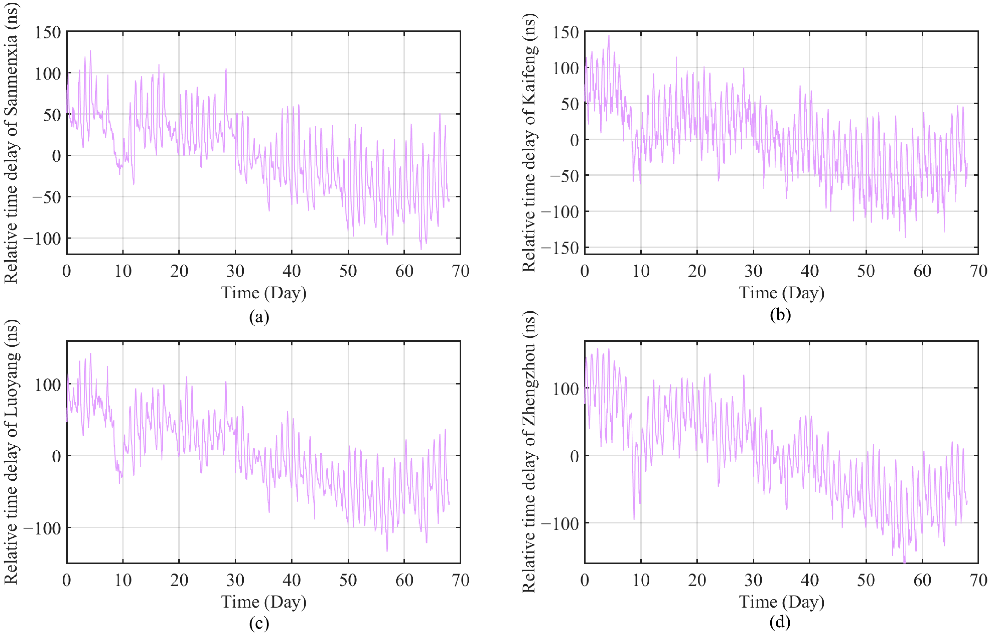
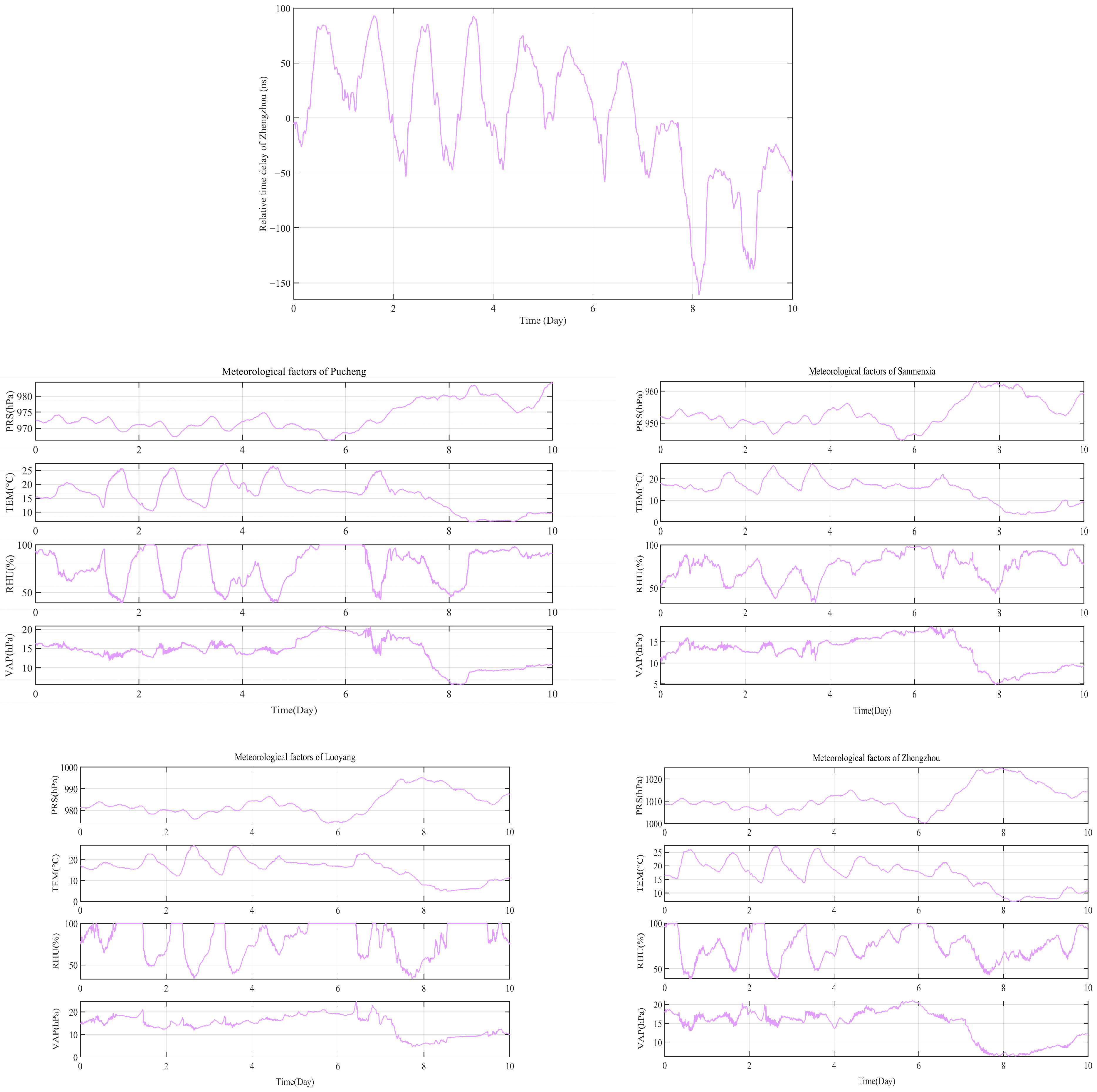
Figure 4 shows the schematic diagram of the fluctuation curve of the effective time-delay measurement value received by Sanmenxia and other differential reference stations from 12 October 2024 to 1 January 2025, after removing the coarse value and abnormal value, subtracting the mean value, and then smoothing filtering and down sampling.
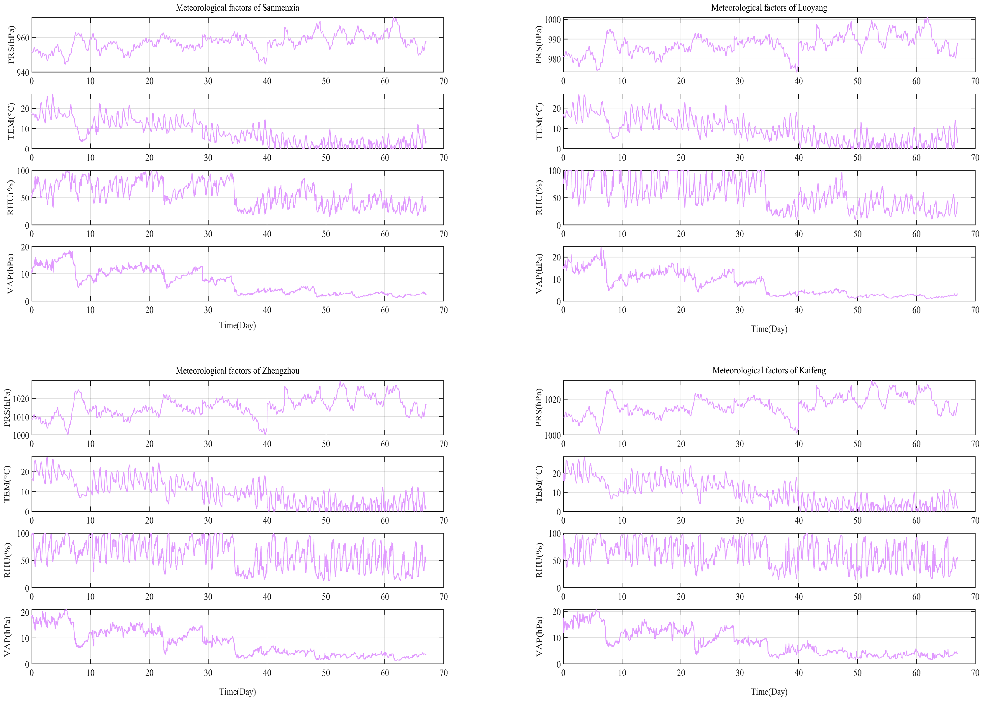
Figure 5 shows the data change curves for the various meteorological factors collected by multiple weather stations on the same propagation path in the same time period (only parts of the meteorological factors are drawn due to space limitations).
According to the visual display in
Figure 4 and
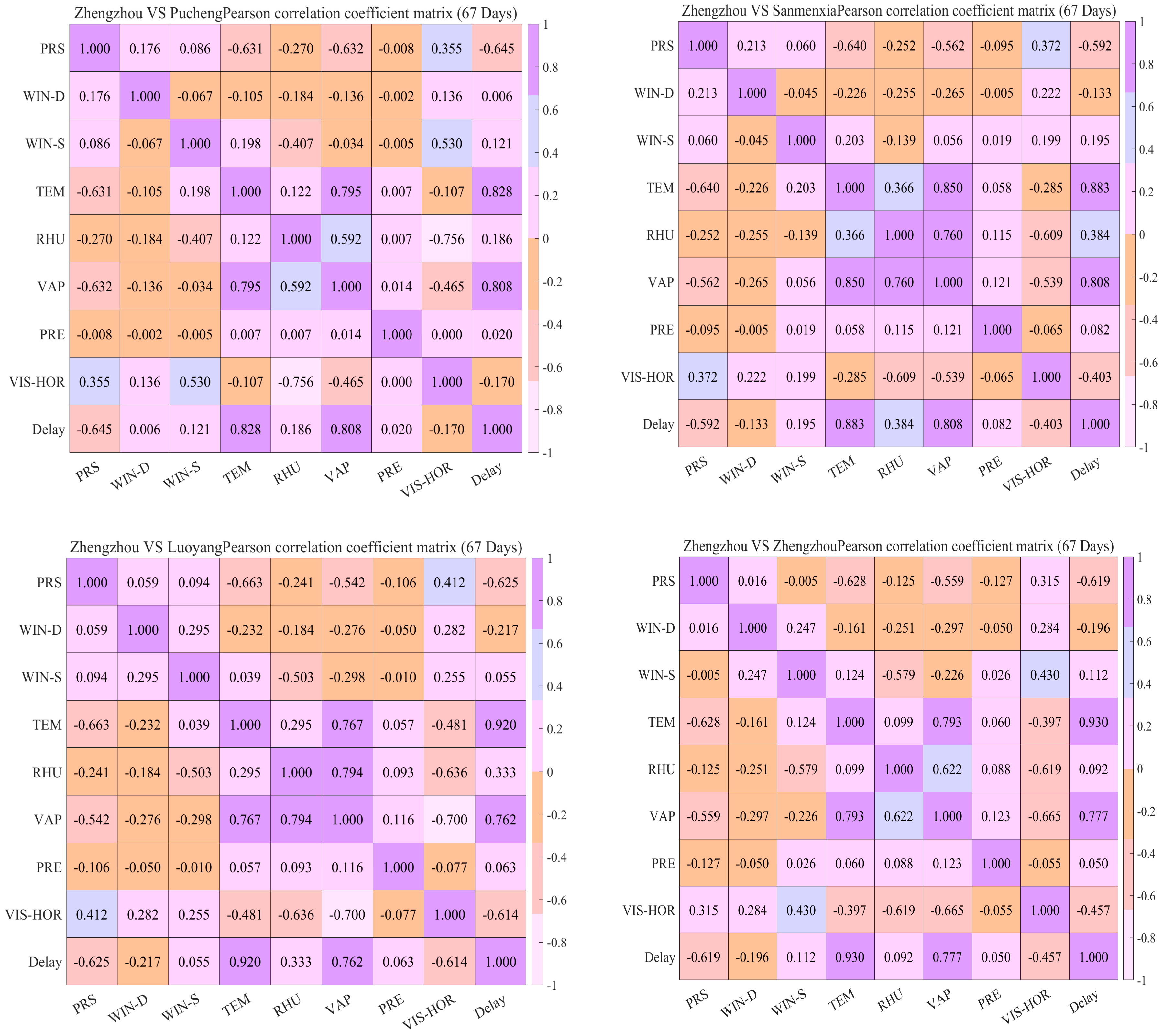
Figure 5, it can be observed that there is a strong correlation between temperature, air pressure, vapor pressure, and time-delay variation, and the correlation between the signal propagation delay and temperature data variation is more obvious. To further explore this relationship, taking the Zhengzhou differential reference station as an example, a long-term correlation analysis was conducted on the valid propagation delay data from 12 October 2024 to 1 January 2025 (67 days) with the relevant meteorological element observation data from multiple national-level meteorological stations along the signal propagation path. The results are shown in
Figure 6.
Due to space limitations, this paper only analyzes the propagation delay data of Zhengzhou station, and the results of the other three stations are not much different. In the long-distance transmission scenario, the temperature difference above 20 °C leads to the time-delay fluctuation with a peak value of more than 250 ns. This result further validates the theory of the influence of meteorological factors on the propagation delay of eLoran signals in
Section 2.2, and is consistent with the relevant conclusions in previous studies [
21,
22]. It can also be proved in the literature [
41,
42,
43,
44,
45,
46] that the long-term change in the propagation delay of eLoran signal has a strong correlation with temperature, vapor pressure, and atmospheric pressure, and the absolute value of the Pearson correlation coefficient reaches more than 0.9, 0.8, and 0.6, respectively. In addition, as the distance between the weather station and the broadcasting station continues to increase, the long-term correlation coefficient of temperature also increases, while the correlation coefficient calculated with the local temperature of Zhengzhou reaches 0.932. At this time, the propagation delay and the temperature are almost linear. In the long run, the average temperature of each place on the path is decreasing. As the distance increases, the cumulative effect of temperature on propagation delay is consistent everywhere, which verifies the conclusion in
Section 3.1.
As can be seen from
Figure 6, the correlation coefficient value between air pressure and propagation delay does not satisfy the above conclusion, because in the long run, the change in air pressure in all parts of the path does not satisfy the same change direction as temperature in the long-distance propagation scenario, so the cumulative effect on the path is not obvious. Furthermore, all kinds of meteorological factors are not independent of each other, but instead have a complex nonlinear coupling relationship, and this nonlinear coupling relationship also causes the fluctuation in the correlation coefficient value. The above findings not only consolidate the previous research foundation, but also preliminarily prove the correctness of the theory in
Section 3.1.
3.3.2. Short-Term Correlation Analysis
From the results of long-term correlation analysis, it can be inferred that the temperature difference changes dramatically due to the change of day and night or the temperature difference of some areas heating up and some areas cooling down along the transmission path. Alternatively, the propagation delay of the eLoran signal will also change drastically in severe weather, such as heavy precipitation, lightning, and strong winds. Therefore, it is necessary to analyze the short-term correlation between the meteorological factors on the propagation path and the propagation delay of eLoran signal.
Figure 7 shows the short-term eLoran signal propagation delay data of Zhengzhou differential reference station within 10 days (from 12 October 2024 to 21 October 2024) and the change curve of the meteorological factor data received by multiple weather stations on the signal propagation path during the corresponding time period. The data processing method is the same as the above.
From the above eLoran signal propagation delay data and the meteorological factor change data curve of weather stations along the way, it can be seen that the time-delay value of Zhengzhou station (400 km) shows dramatic changes within a day, and the fluctuation range can reach more than 150 ns in some days. In addition, the daily change trend of the time-delay value has a certain periodicity, rising slowly every morning. It reaches the maximum value of the day around 2 pm to 3 pm, then slowly decreases and reaches the lowest value in the early morning. This change is consistent with the temperature change in the corresponding location and is opposite to the humidity change.
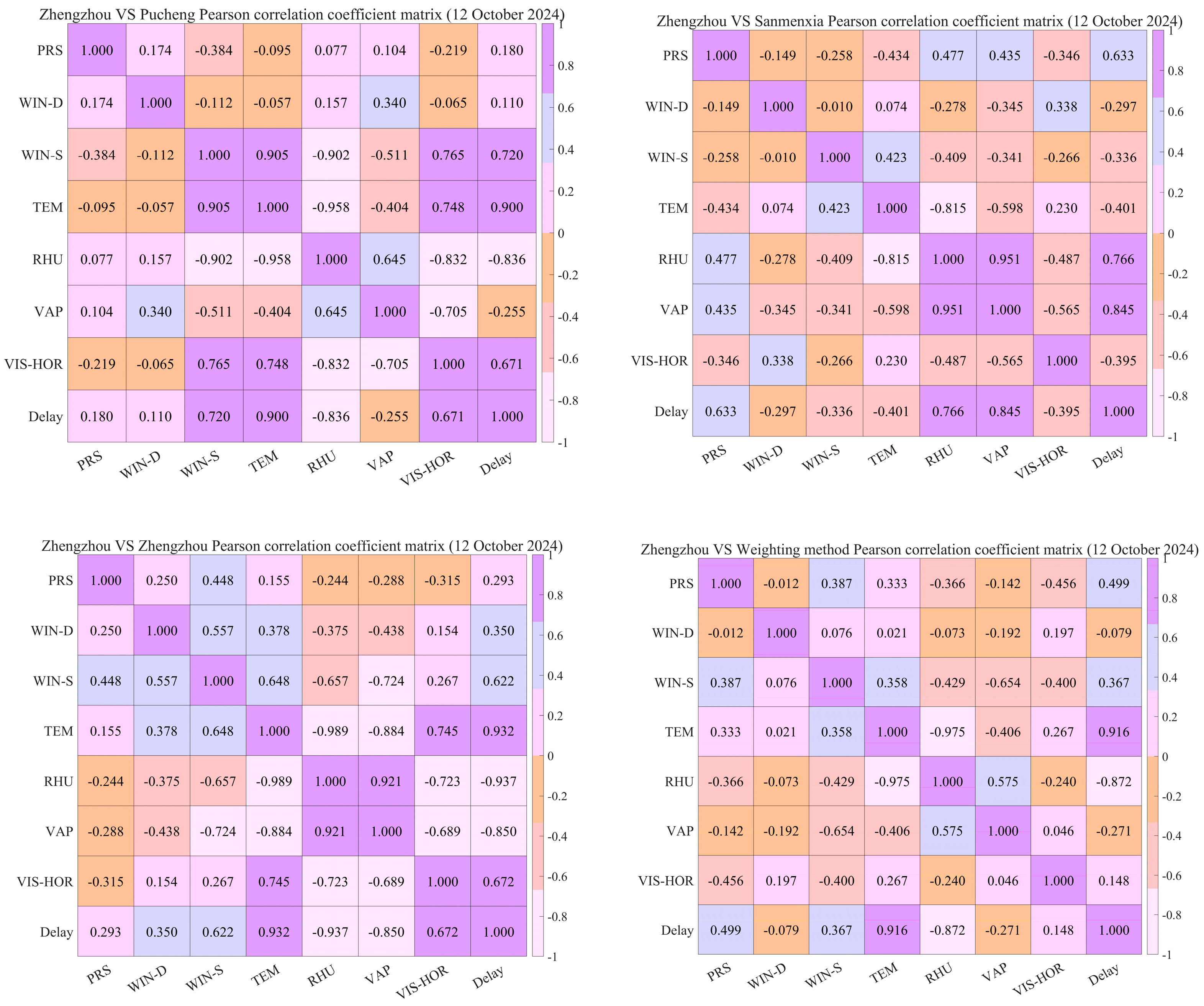
Figure 8 shows the results of the short-term Pearson correlation coefficient matrix analysis of the time-delay data of Zhengzhou station on 12 October 2024 and the meteorological data of some weather stations on the path.
Table 1 shows the Pearson correlation coefficients between temperature and humidity of Zhengzhou station and multiple weather stations along its path and the measured values of time-delay. Due to the large amount of data, only the two meteorological factors with large correlation coefficients are listed in the table, and the correlation coefficients of other meteorological factors not listed are similar.
The data show that the linear correlation between temperature, humidity, and propagation delay is high, the absolute value can reach more than 0.9 on some days, the temperature is positively correlated with the delay fluctuation, and the humidity is negatively correlated with the delay fluctuation. For example, on the first day, because Pucheng, Luoyang, and Zhengzhou are all heating up, the temperature of Sanmenxia has a small change, and the humidity also has a similar situation. The time-delay value fluctuates greatly on that day, but the correlation between the time-delay of Zhengzhou and the meteorological data of Sanmenxia is small, and the correlation coefficient value returns to normal after path weighting. This also proves the correctness of the correlation coefficient algorithm based on path weighting. On the sixth day, due to the precipitation, the temperature change in Pucheng, Sanmenxia, and Luoyang is very small, and the humidity is maintained at the maximum value for a long time, resulting in poor temperature correlation and positive humidity correlation. Moreover, the temperature in Zhengzhou fluctuates to a certain extent, which is the reason why the correlation coefficient becomes larger in Zhengzhou on that day. The sign of the humidity-weighted correlation coefficient is still positive and the temperature correlation coefficient is small, which indicates that under such long-distance propagation conditions, it is far from enough to calculate the path-weighted correlation coefficient by only considering the meteorological data of four weather stations. This is the limitation of the algorithm, and it is necessary to consider the data of weather stations with larger density in the future.
3.4. Summary
Through the above theoretical analysis, it can be seen that the cumulative effect of meteorological factors on the propagation delay of eLoran signals shows significant spatial heterogeneity with the increasing propagation distance. In the short-distance propagation scenario, the change in the meteorological factors in the same direction can cause the delay fluctuation and the path length linear relationship. In the long-distance transmission scenario, the difference of regional meteorological factors will lead to the superposition of positive and negative contributions of time-delay fluctuations, and the final cumulative effect shows nonlinearity or uncertainty. Based on this, the Pearson correlation coefficient algorithm based on distance weighting was proposed. By using the meteorological data of multiple weather stations on the path, the interference of local meteorological abrupt changes in the overall correlation analysis could be effectively solved. At the same time, the strong correlation between temperature, humidity, and propagation delay during long-distance propagation was revealed, which verified the correlation between meteorological factors and time-delay.
The analysis of the measured data further shows that the short-term time-delay fluctuation is closely related to the local temperature and humidity variation, and the long-term variation is affected by the cumulative evolution of regional temperature and humidity. Moreover, the path-weighted algorithm shows stronger robustness in long-distance scenarios. However, extreme weather or local meteorological abrupt change will still cause the sign reversal of correlation coefficient, which reflects the complexity of nonlinear coupling between meteorological factors. In addition, due to the lack of spatial resolution of the available meteorological data, the model has limitations in accurately describing the time-delay changes caused by meteorological changes on long-distance paths.
4. Experimental Results and Performance Analysis
According to the calculation formula of propagation delay, due to the change in meteorological factors, the value of the propagation delay also changes. Propagation delay is affected by the explicit or implicit effects of meteorological factors, and there are complex nonlinear relationships between meteorological factors, so it is difficult to use simple mathematical analytical models to directly model propagation delay. The literature [
47,
48,
49,
50] uses neural networks to establish the relationship model between meteorological factors and propagation delay and effectively predicts the signal propagation delay. Based on these, we choose the BP neural network to facilitate the comparison and evaluation of the prediction effect of propagation delay in long-distance scenarios within the existing research context. This study intends to establish the corresponding BP neural network fitting model for a variety of meteorological factors at multiple weather stations on the path in the long-distance transmission scenario. The input of the model is various meteorological factor data, such as temperature, humidity, air pressure, precipitation, etc., at a certain location along the path. The number of nodes in the input layer needs to be determined specifically based on the situation of the prediction task. The output of the model is the propagation delay data of the location to be predicted, with the number of nodes being 1. Experience shows that deep networks do not significantly improve the performance of the prediction model in the current application scenario and are prone to overfitting problems. Therefore, it is better to limit the number of hidden layers to 1 or 2. Then, the number of nodes in the hidden layer is estimated based on the empirical formula
, where d is the number of nodes in the input layer, l is the number of nodes in the output layer, and m is an integer within the range of 1 to 10. Different BP neural network models are constructed, and the optimal number of nodes in the hidden layer is determined through the method of experiments and parameter adjustment based on experience. There are three common activation functions, namely sigmoid, tanh, and RELU [
51,
52,
53,
54,
55,
56,
57,
58,
59]. After testing, it was found that the sigmoid activation function performed the best among the three activation functions. Therefore, the activation function of all BP neural network prediction models in this paper is taken as the sigmoid function. A total of 14 different models were established in this chapter, all using the method of experiments and parameter adjustment based on experience. The number of hidden layers and nodes, learning rate, and learning times were set, respectively. Due to space limitations, the models presented in the article are the optimal parameter models selected through the trial-and-error method. In
Section 4.4, the settings of the input layer, output layer, hidden layer, and other related parameters of the multi-meteorological factor BP neural network (PSLZM-BPNN) from Pucheng to Sanmenxia, Luoyang, and Zhengzhou are described in detail. The basic principle of BP neural network can be formally represented as the structure in
Figure 9.
In this chapter, the eLoran signal propagation delay data of differential reference stations, such as Zhengzhou, and multiple meteorological factors on the corresponding propagation path are combined to establish different BP neural network prediction models from three perspectives for analysis and comparison. After the model is successfully trained, all kinds of meteorological factors in the test set are used as the input of the model to obtain the output value of the model. Finally, it is compared with the real value to test the performance of the model.
4.1. Data Acquisition and Processing
eLoran signal broadcasting station: Pucheng BPL long-wave timing station;
Differential reference station acquisition equipment: eLoran signal long-wave timing receiver (KTL-202A-F), long-wave receiving antenna (KTL-606B-DF14), high-precision GNSS timing receiver (IME-GNSS200T-2), GNSS receiving antenna, time interval counter (MTIM712), etc.
Collection points: four differential reference stations in Sanmenxia, Luoyang, Zhengzhou, and Kaifeng;
Collection time: 82 days (from 12 October 2024 to 1 January 2025, with valid data retained for 67 days);
Data resolution: 1 per second.
- 2.
Meteorological data.
Collection points: Pucheng, Sanmenxia, Luoyang, Zhengzhou, and Kaifeng (five weather stations);
Acquisition time: same as eLoran signal propagation delay acquisition time;
Data types: temperature, humidity, air pressure, precipitation, vapor pressure, surface temperature, wind direction, wind speed, and visibility;
Data resolution: 1 per minute.
Given the relevant regulations on the security of meteorological data, higher spatial resolution meteorological data cannot be obtained through public or conventional research channels at the present stage. However, the resolution level of this data is already sufficient to support the analysis and evaluation of the prediction accuracy of the propagation delay of the impact of meteorological data spatial resolution.
- 3.
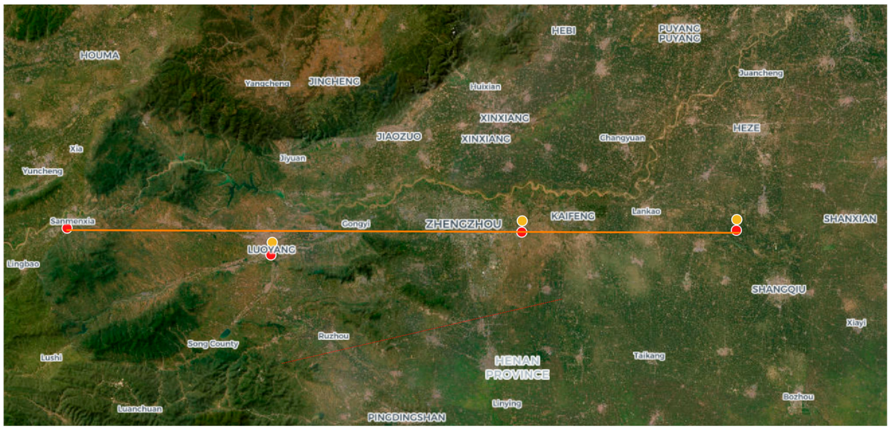
This study focuses on the problem of predicting the propagation delay of eLoran signals in long-distance transmission scenarios. The selected differential reference stations are mainly based on the following three points: Firstly, the selected differential reference stations meet the conditions for long-distance signal transmission, and the distance distribution between the stations is relatively uniform; secondly, the geographical locations of each reference station are nearly collinear, which conforms to the physical laws of radio timing signal propagation; thirdly, the terrain undulation and meteorological conditions in the area traversed by the selected path show significant diversity, making the data collected on this path more representative. Therefore, four differential reference stations in Henan Province, namely Sanmenxia, Luoyang, Zhengzhou, and Kaifeng, are selected as the research objects.
Figure 10 shows the distribution of meteorological stations along the propagation path from BPL long-wave timing station in Pucheng to the eLoran signal differential base station in Kaifeng, where the red dot clearly marks the specific location of each meteorological observation station, the yellow dot is the location of the differential reference station, and the red star is the location of the BPL long-wave timing station in Pucheng. Through this figure, the spatial layout of the weather station and its relationship with the signal propagation path can be intuitively understood, which provides an important spatial reference for the establishment of the propagation prediction model and data analysis below.
4.2. Influence of the Number of Input Factors on the Propagation Delay Prediction Model
In this section, three meteorological factors with a large correlation, namely temperature, humidity, and pressure, are, respectively, used as the single input of a BP neural network, the BP neural network prediction model based on single factor is constructed, and the corresponding linear model is established at the same time. Then, two and three of the three factors are used as multiple inputs, and more meteorological factors are added on the basis of the three meteorological factors as multiple inputs to construct a multi-factor neural network model, train and adjust the parameters of the neural network, and conduct comparative analysis and performance evaluation. The influence of the number of meteorological factors input into the prediction model on the prediction accuracy of signal propagation delay was explored, and the influence of adding other meteorological factors with less correlation on the model is explored.
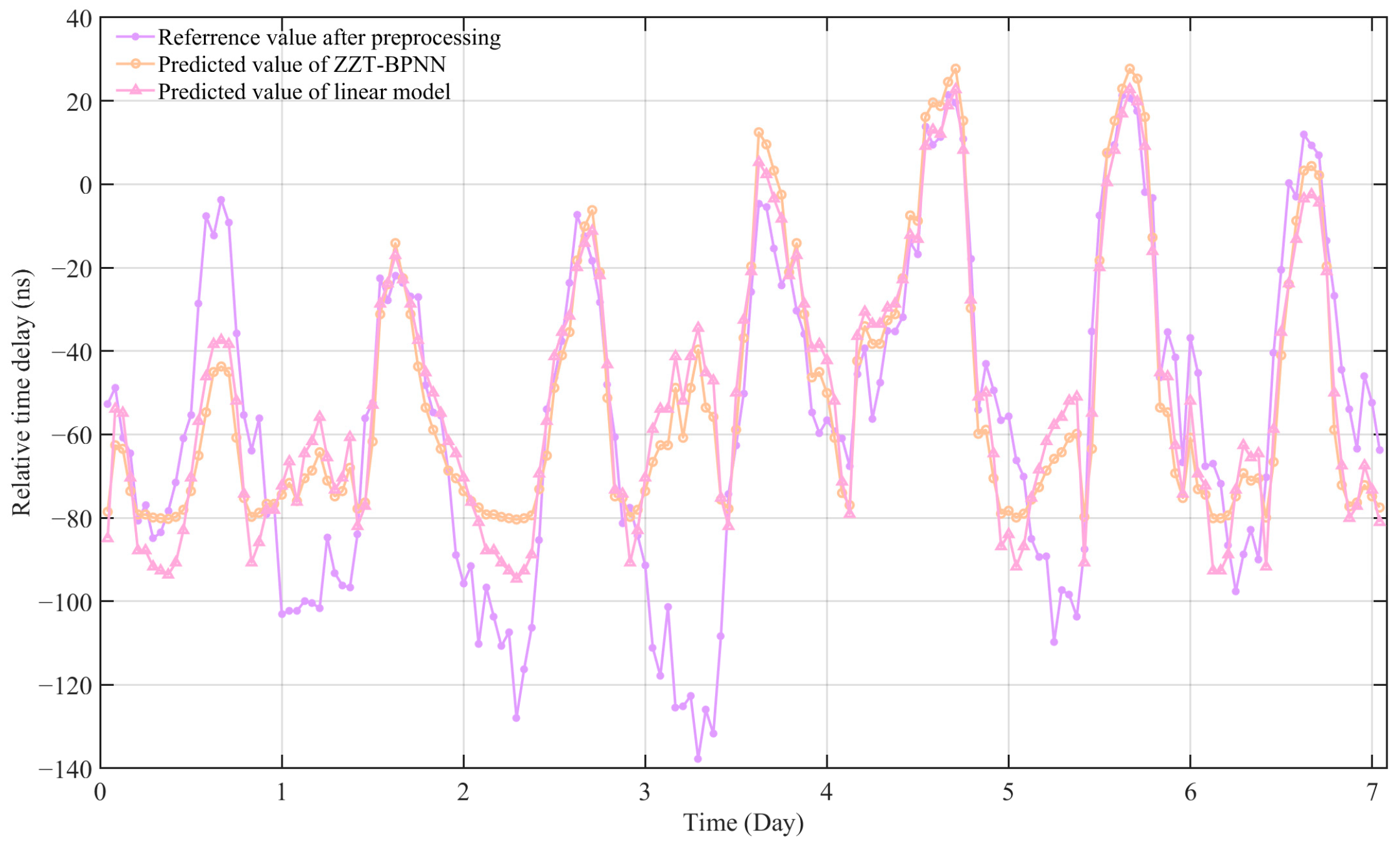
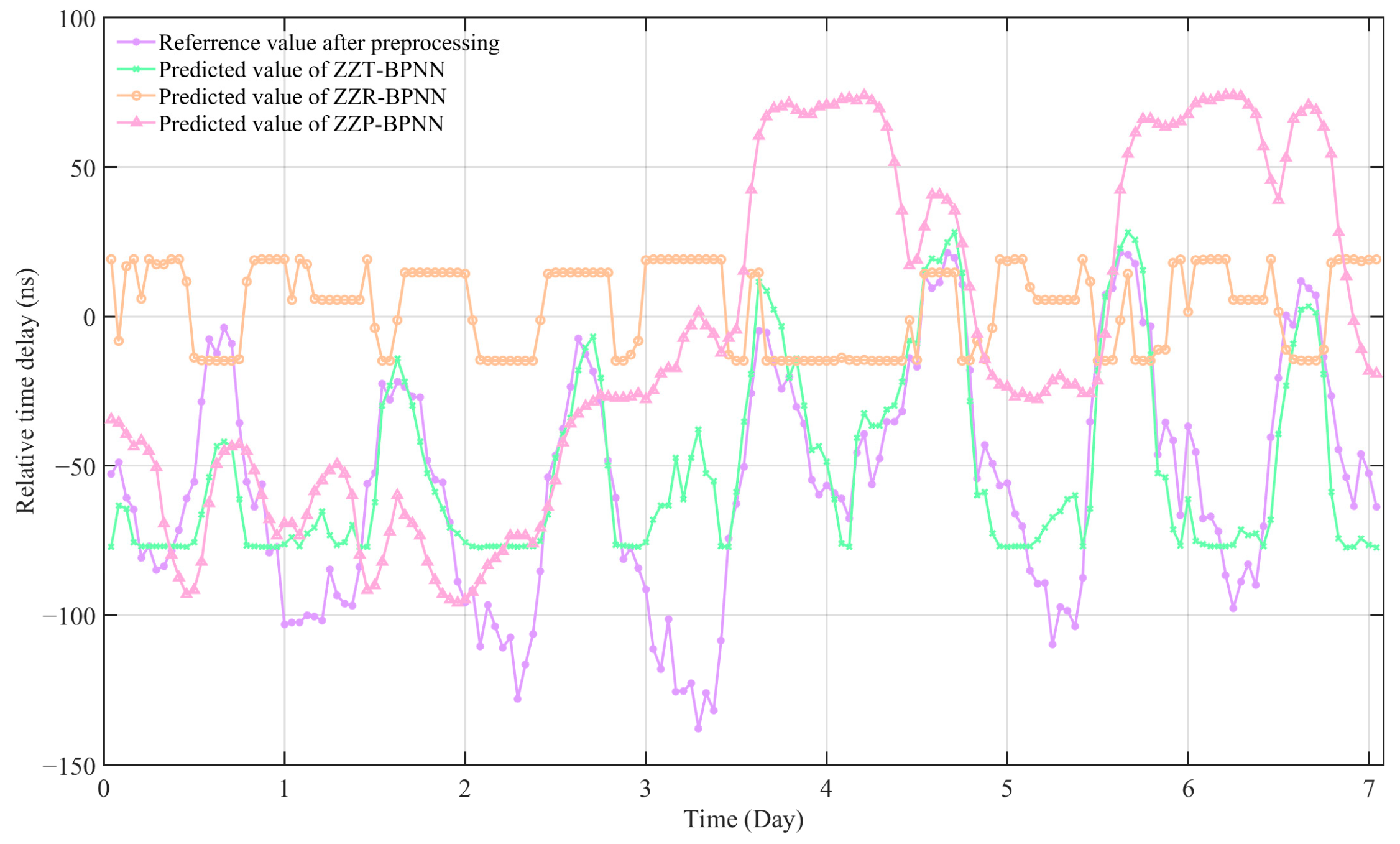
Firstly, 60 days (about 90% of the total data) were selected from the delay data of the Zhengzhou difference station as the training set to construct the BP neural network model, and the remaining 7 days (about 10% of the total data) were used as the test set. In the model design, the temperature, humidity, and air pressure of Zhengzhou weather station were taken as single input, and a variety of BP neural network models were built by adjusting the number of hidden layers and the number of hidden layer nodes. Then, these factors were used as the input of the linear model to build a variety of linear prediction models. Subsequently, the performance of these models was analyzed based on the evaluation criteria of minimum root mean square error (RMSE) and minimum mean absolute error (MAE), and their test results are shown in
Figure 11 and
Figure 12. For ease of presentation, the optimal parameter models are named as follows: Zhengzhou temperature BP neural network (ZZT-BPNN), Zhengzhou humidity BP neural network (ZZR-BPNN), and Zhengzhou air pressure BP neural network (ZZP-BPNN).
From the above results, it is found that when only single meteorological factor data of a single weather station is considered, the number of hidden layers has little influence on the fitting results, and the model using temperature data has the best fitting effect. As shown in
Figure 11, the BP neural network model based on temperature factor shows a higher degree of fit than the humidity and pressure models. Specifically, the root mean square error (RMSE) and mean absolute error (MAE) of the ZZT-BPNN model were 24.4285 ns and 17.8134 ns, respectively, and the corresponding indexes of the ZZR-BPNN model were 74.1847 ns and 62.2449 ns, respectively. The corresponding indexes of ZZP-BPNN model were 72.1645 ns and 58.1177 ns, respectively.
In addition, according to the test results, the RMSE of the temperature linear model was 24.4840 ns, and the MAE was 17.4091 ns, which was slightly worse than the ZZT-BPNN model, but better than the BP model of humidity and pressure. At the same time, the performance of the two linear models of humidity and air pressure were not as good as their corresponding BP neural network models, and the performance of the two linear models was not as good as that of the temperature linear model. This is because the linear correlation between temperature and propagation delay was more obvious, so the prediction effect of their corresponding models was also significantly better. This result further indicates the superiority of the BP model in dealing with complex nonlinear relationships.
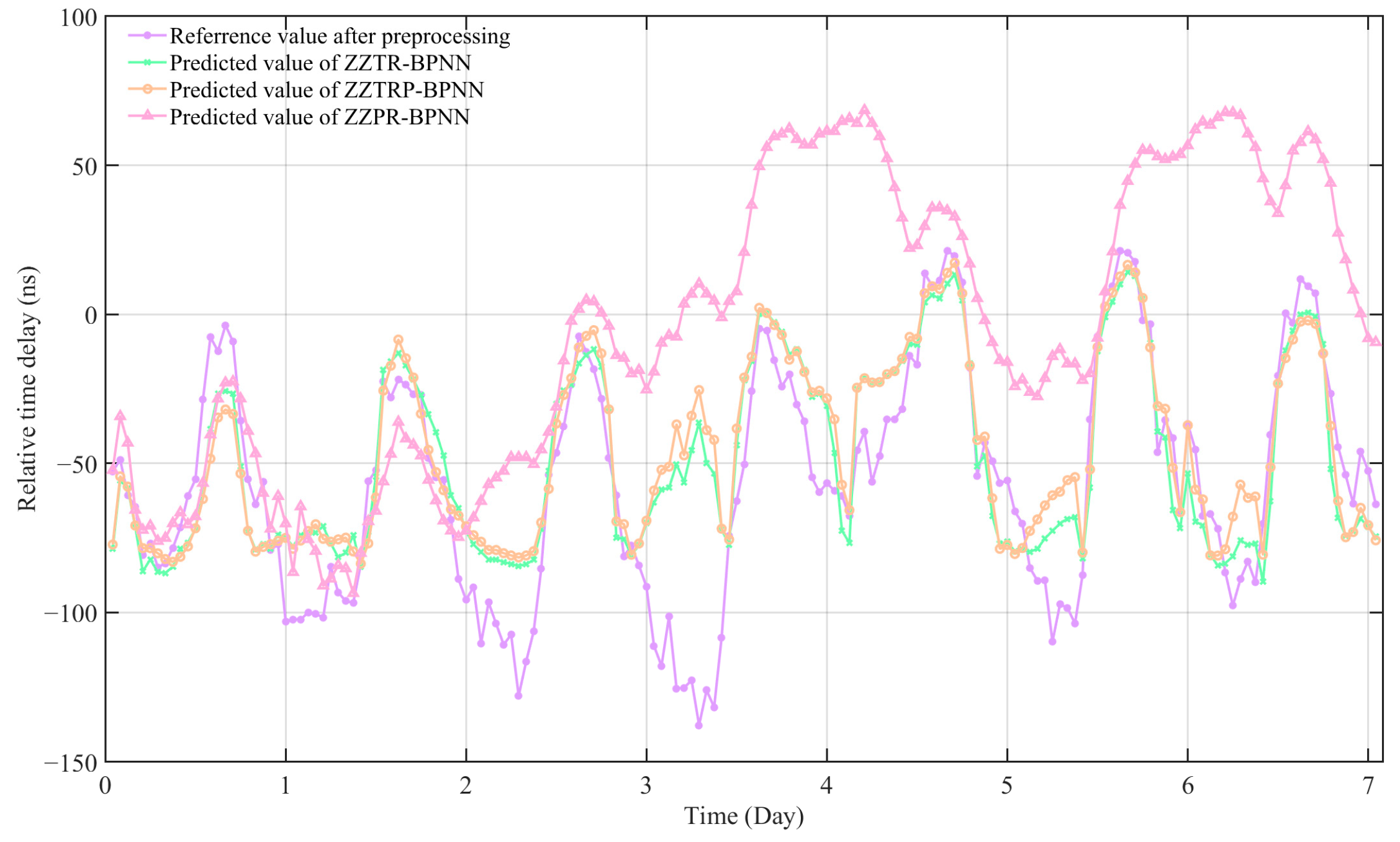
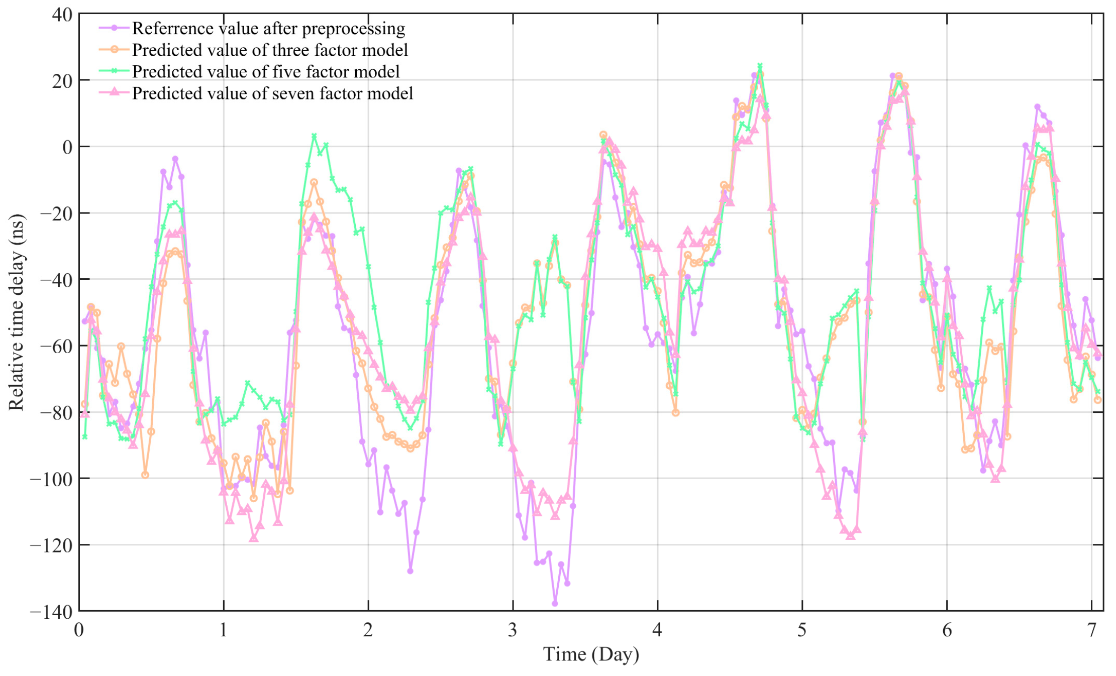
In order to explore the comprehensive influence of multiple meteorological factors on propagation delay, two of the three factors that had a large impact on the delay were combined as inputs, and then the three factors with the largest impact were used as inputs to compare the performance of the four models. Finally, based on the model with three factors as input, more meteorological factors were added to compare the performance of these models. The prediction effect of the model is shown in
Figure 13 and
Figure 14. For ease of presentation, the optimal parameter models are named as follows: Zhengzhou temperature-humidity BP neural network (ZZTR-BPNN), Zhengzhou temperature–air pressure BP neural network (ZZTP-BPNN), Zhengzhou baric–humidity BP neural network (ZZPR-BPNN), Zhengzhou temperature–humidity BP neural network (ZZTRP-BPNN) (three factor model), Zhengzhou temperature–humidity–air pressure–wind speed–wind direction BP neural network (5-factor model), and Zhengzhou temperature–humidity–air pressure–wind speed–wind direction–vapor pressure–precipitation BP neural network (7-factor model).
The experimental results show that the root mean square error (RMSE) and mean absolute error (MAE) of the ZZTR-BPNN model are 24.4377 ns and 18.3320 ns, respectively, and that the performance of the ZZTR-BPNN model is the best among the two-factor input models. The root mean square error (RMSE) and mean absolute error (MAE) of the ZZTRP-BPNN three-factor model were 23.7410 ns and 16.7570 ns, respectively. The corresponding indexes of the five-factor model were 28.3561 ns and 19.4958 ns, respectively. The corresponding indexes of the seven-factor model were 12.7518 and 10.0285, respectively. It can be seen that the input of the two-factor model is the best combination of temperature and humidity, and the three-factor model has a certain improvement in prediction ability compared with the single-factor model. On the basis of the three influential factors as input, by introducing more meteorological factors as input, the prediction ability of the model will not be significantly improved, and the performance will decrease, which is caused by the introduction of more irrelevant factors. However, with the introduction of more influential meteorological factors, the prediction effect has been significantly improved. By comparing the results of the multi-factor prediction model, it can be seen that adding more irrelevant factors will lead to greater complexity of the model, consume more computing resources, and reduce the model’s performance. Therefore, it is necessary to reduce the dimensionality of the data before establishing the prediction model.
4.3. Influence of Prediction Distance on Propagation Delay Prediction Model
All the prediction models established in the previous section do not consider the problem of distance increase. Therefore, this section builds the meteorological data characteristic matrices of Pucheng–Sanmenxia, Pucheng–Luoyang, Pucheng–Zhengzhou, and Pucheng–Kaifeng, respectively. The meteorological data characteristic matrices corresponding to these different distance difference stations are used as the input of the BP neural network to train and adjust the neural network parameters. BP neural network prediction models based on different distances are constructed to predict the signal propagation delay of Zhengzhou and other differential reference stations, respectively. The models are compared and analyzed, and their performance is evaluated to explore the influence of meteorological factors on the prediction accuracy of the signal propagation delay prediction model with the increase in signal receiving distance.
Firstly, 60 days (about 90% of the total data) were randomly selected from the observation data of the five observation points as the training set to construct the BP neural network model, and the remaining 7 days (about 10% of the total data) of each data set were used as the test set of the corresponding data. In the model design, a variety of BP neural network models were constructed with the input of a variety of meteorological factor feature matrices of the Pucheng–Sanmenxia, Pucheng–Luoyang, Pucheng–Zhengzhou, and Pucheng–Kaifeng weather stations. The performance of each class of models was subsequently analyzed, and the test results are shown in
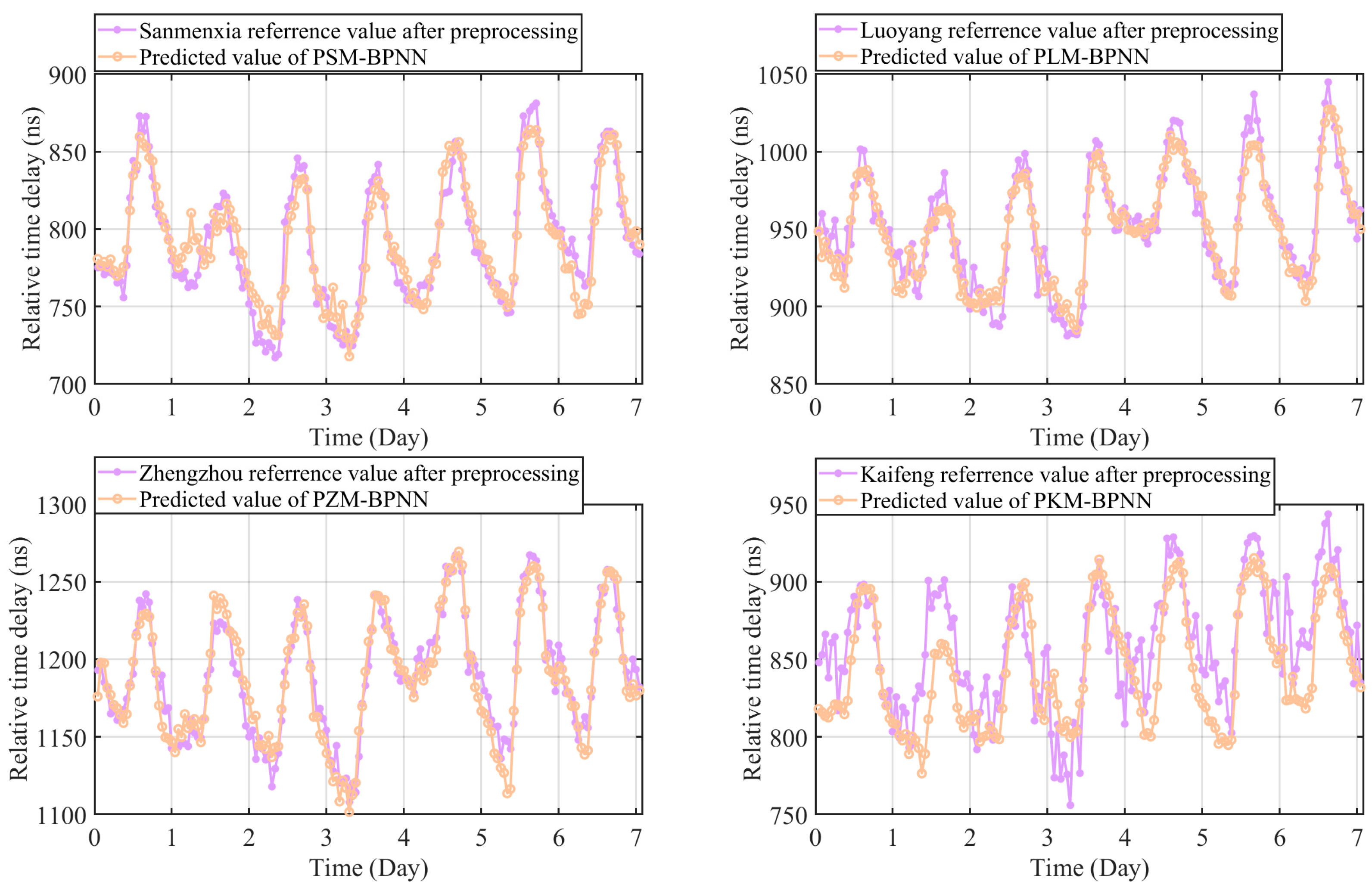
Figure 15. For ease of presentation, the optimal parameter models are named as follows: Pucheng–Sanmenxia multi-meteorological factor BP neural network (PSM-BPNN), Pucheng–Luoyang multi-meteorological factor BP neural network (PLM-BPNN), Pucheng–Zhengzhou multi-meteorological factor BP neural network (PZM-BPNN), and Pucheng–Kaifeng multi-meteorological factor BP neural network (PKM-BPNN).
According to the prediction results, it is found that when only considering the propagation delay of the predicted determined distance, the parameters have little influence on the fitting results. From the display effect in
Figure 15, the root mean square error (RMSE) and mean absolute error (MAE) of the PSM-BPNN model are 14.0896 ns and 11.1667 ns, respectively, and the corresponding indicators of the PLM-BPNN model are 12.408 ns and 9.7165 ns, respectively. The corresponding indexes of the PZM-BPNN model are 12.2152 ns and 9.6825 ns, respectively. The corresponding indices of the PKM-BPNN model are 28.4608 ns and 23.2206 ns, respectively. The prediction effect of Zhengzhou station is the best, and the prediction effect of Kaifeng station is the worst. When the prediction distance is less than the distance between the broadcast station and Zhengzhou station, the prediction effect is better and improves with the increase in the prediction distance. This is because the dramatic change in local meteorological factors leads to the change in the time-delay data in this place and is greatly affected by the local weather, while the cumulative influence on the path has little impact on the data fluctuation, so the use of local meteorological data for prediction has a better effect. The performance of the PKM-BPNN model is poor. This is because the cumulative influence of the changes in meteorological factors in different regions on the signal propagation path on the signal propagation delay becomes longer with the signal propagation distance, and the local meteorological fluctuation is small, so the effect of using only local meteorological data to predict the propagation delay is poor. Therefore, when a certain number of meteorological factors are used as the input of the prediction model, as the signal propagation path continues to become longer, if only the meteorological data of the signal transmitting place and receiving place are used to construct the prediction model, the fitting accuracy of the prediction model under the long-distance condition will decrease. This result verifies the conclusion in
Section 3.1.
4.4. Influence of the Number of Weather Stations on the Propagation Delay Prediction Model
The model established in the previous section only considers the influence of meteorological factors in both transmitting and receiving places on the propagation delay and ignores the problem of the impact of regional cumulative changes in the meteorology on the propagation path. This section takes the path from the Pucheng to Zhengzhou differential reference station as an example by adding more weather station data on the path as the input of the BP neural network and explores the effect of the increase of the number of weather stations on the path. The influence of regional meteorological changes on the propagation path on the prediction accuracy of signal propagation delay model is examined.
From the observation data of the four observation points, 60 days of meteorological data and propagation delay data (about 90% of the total data) were randomly selected as the training set to construct the BP neural network model, and the remaining 7 days of each data set (about 10% of the total data) were used as the test set of the corresponding data. A variety of BP neural network models were built by using a variety of meteorological factor characteristic matrices of Pucheng–Zhengzhou, Pucheng–Sanmenxia–Zhengzhou, and Pucheng–Sanmenxia–Luoyang–Zhengzhou meteorological stations to predict the signal propagation delay of the Zhengzhou differential reference station; the models were compared and analyzed, and their performance was evaluated. The test results are shown in
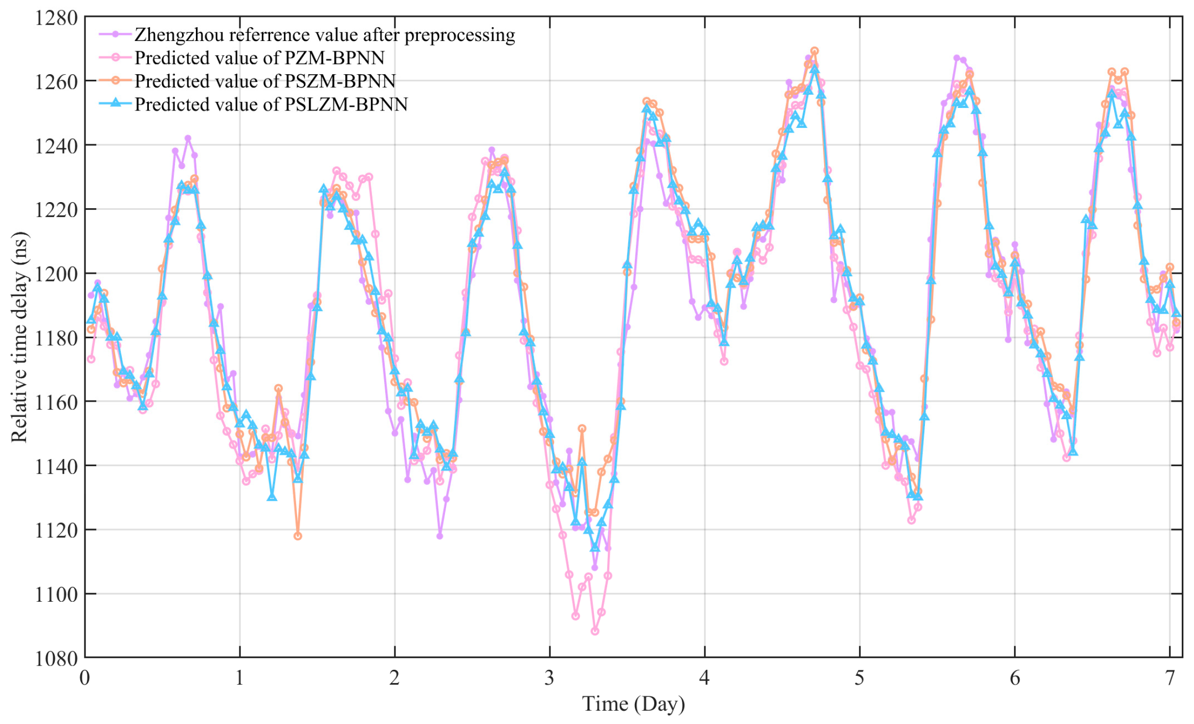
Figure 16. The relevant parameters of the BP neural network for the multi-weather factor prediction from Pucheng to Sanmenxia, Luoyang, and Zhengzhou are as follows: The input layer of the model has 1 node, and the total number of nodes is 28. The input data consist of seven weather factor data from Pucheng, Sanmenxia, Luoyang, and Zhengzhou. The output layer of the model has one node, and the output data is the propagation delay data of Zhengzhou. The number of hidden layers is set to two. The optimal number of nodes in the hidden layer is determined through experimental and empirical adjustment methods, resulting in values of 12 and 5, respectively. The activation function is the sigmoid function, the learning rate is 0.001, and the number of learning iterations is 10,000. For ease of presentation, the optimal parameter models are named as: follows Pucheng–Zhengzhou multi-meteorological factor BP neural network (PZM-BPNN), Pucheng–Sanmenxia–Zhengzhou multi-meteorological factor BP neural network (PSZM-BPNN), and Pucheng–Sanmenxia–Luoyang–Zhengzhou multi-meteorological factor BP neural network (PSLZM-BPNN).
According to the display effect in
Figure 16, the BP neural network model based on the data of the Pucheng–Sanmenxia–Luoyang–Zhengzhou–Kaifeng stations shows a higher degree of fit than other models. Specifically, the root mean square error (RMSE) and mean absolute error (MAE) of the PSLZM-BPNN model are 11.5441 ns and 8.8986 ns, respectively, which are the best, and the corresponding index of the PSZM-BPNN model is 12.1525 ns and 9.6315 ns. The corresponding indexes of the PZM-BPNN model are 14.6309 ns and 10.3534 ns, respectively. This is due to the fact that as the propagation path becomes longer, the cumulative influence of meteorological changes in multiple regions on the path on the time-delay becomes larger. It is far from enough to only consider the influence of meteorological factors at the beginning and end point when modeling. The time-delay prediction model will have higher data fitting accuracy as the spatial resolution of the weather station data becomes more accurate. In the later stage, more weather station data on the path will be considered to improve the data fitting accuracy.
In summary, the experimental results show that when temperature is used as the single factor input, the prediction model based on BP neural network performs best in the delay prediction task, and its nonlinear advantage is significantly improved compared with the traditional linear model. The prediction accuracy of the multi-factor model does not increase unbounded with the increase in the dimension of meteorological data. When several strongly correlated factors are used for prediction, the prediction accuracy of the model may be weakened by continuing to increase the meteorological factors, which reflects the necessity of feature screening in the early stage. In the long-distance transmission scenario, the spatial resolution has a significant impact on the prediction error, and the introduction of the intermediate weather station data can reduce the prediction error of the long-distance prediction model. In addition, the comparison of models with different propagation distances shows that local meteorological fluctuations have a more significant impact on the time-delay in short-distance scenarios, while the synergy of meteorological changes in multiple regions of the path should be comprehensively considered in long distance scenarios.
5. Conclusions
The influence of the fluctuation of meteorological factors on the propagation delay estimation of eLoran signals over medium and long distances is a core challenge to improve the accuracy of system timing. Aiming at the problem of insufficient time-delay prediction ability of traditional models when using multi-factor data of multiple weather stations in long-distance propagation scenarios, this paper proposes a propagation delay prediction model based on multi-station meteorological observation data and a BP neural network for long-distance propagation scenarios.
Firstly, the dynamic influence mechanism of meteorological factors on propagation delay was revealed by theoretical modeling, and the quantitative action law of time-varying characteristics of the atmospheric refractive index and the ground equivalent electrical conductivity on the time-delay component was clarified. Secondly, based on the observation data of multiple weather stations, the Pearson correlation coefficient analysis method based on distance weighting was innovatively adopted to study and demonstrate the relationship between the changes in meteorological factors, delay fluctuations, and path length in short-distance transmission scenarios, as well as the cumulative effect of meteorological factors on propagation delay in long-distance transmission scenarios. In addition, the strong correlation between meteorological factors, such as temperature and humidity, and propagation delay was revealed under long-distance propagation conditions, and the complex coupling mechanism between meteorological factors and propagation delay was further verified. On this basis, the single-factor and multi-factor BP neural network models for long-distance propagation scenarios were constructed. At the same time, from the two dimensions of prediction distance and the number of used weather stations, a multi-station meteorological data time-delay prediction model based on long-distance propagation path was established, which effectively improves the prediction accuracy of propagation time-delay.
However, this study still has the following limitations: the spatial and temporal resolution of the meteorological data is low, the data feature selection method needs to be optimized, the long-term data in years is lacking to verify the seasonal variation in propagation delay, the traditional model architecture is still used, and the actual data are not optimized. Therefore, future research directions can be carried out from the following perspectives.
Firstly, we should increase the spatial density of weather stations or combine meteorological satellite data to use meteorological data with a higher spatial resolution, improve the sampling rate of meteorological data, and improve the monitoring ability of local weather changes.
Secondly, nonlinear correlation analysis of meteorological data and propagation delay data should be carried out, and a new data dimension reduction method should bne used to eliminate irrelevant meteorological data and reduce the complexity of the model.
Thirdly, we should use longer-term observation data and collect time-delay and meteorological data in the spring, summer, autumn and winter for many years, then analyze the fluctuation law of time-delay in different seasons.
Finally, we should design a more efficient prediction model for this prediction task and improve its expressiveness and accuracy in specific scenarios by optimizing the algorithm structure and parameter configuration.

 ,
, 


